Vortex dynamics of charge carriers in the quasirelativistic graphene model : high-energy $\vec{k}\cdot\vec{p}$ approximation

Abstract

Within the earlier developed high-energy-$\vec{k}\cdot\vec{p}$-Hamiltonian approach to describe graphene-like materials the simulations of non-Abelian Zak phases and band structure of the quasi-relativistic graphene model with a flavors number $N=3$ have been performed in approximations with and without gauge fields (flavors). It has been shown that a Zak-phases set for non-Abelian Majorana-like excitations (modes) in Dirac valleys of the quasirelativistic graphene model is the cyclic group $\mathbf{Z}_{12}$. This group is deformed into $\mathbf{Z}_{8}$ at sufficiently high momenta due to deconfinement of the modes. Since the deconfinement removes the degeneracy of the eightfolding valleys, Weyl nodes and antinodes emerge. We offer that a Majorana-like mass term of the quasirelativistic model effects on the graphene band structure in a following way. Firstly the inverse symmetry emerges at ”switching on” of the mass term, and secondly the mass term shifts the location of Weyl nodes and antinodes into the region of higher energies and accordingly the Majorana-like modes can exist without mixing with the nodes.

I Introduction

Currently, topological graphene-like materials attract great attention due to possibility of implementing robust quantum computing on quantum devices constructed from such materials. Types of topological defects in the band structure of graphene-like materials are diverse: Weyl nodes and antinodes Lu-Shen2017Front-Phys , Weyl nodal (antinodal) lines NatCommunic7-2016Bian , drumhead-like surface flat bands PhysRevX6-2016Muechler ; Honeycomb-KagomeLattice2017 , zero-energy Majorana modes PhysRevX5-2015San-Jose , despite the fact that the crystal structure of all topological materials is either hexagonal or almost hexagonal SangwanHersam2018 . Establishing a mechanism of the influence of the degree of symmetry breaking due to spin-orbit interaction on the type of the band-structure defectiveness is a challenge, but it is extremely important for applications of topological materials. A hindrance to solving this problem lies in impossibility to construct maximally localized Wannier orbitals in a lattice site $i$ for a band structure with topological defects owing to the presence of the defect in the site $i$. Majorana end states were implemented as subgap levels of an atomic chain on the surface of a p-wave superconductor. This system is named a Kitaev’s chain Physics-Uspekhi44-2001Kitaev ; JPhysB40-2007Semenoff . These subgap levels are similar to Shockley or Shiba states bound to electric or magnetic end impurities (see Beenakker ; Peng and references therein) but Shockley or Shiba states do not possess topological stability of vortex states. By connecting three Kitaev’s chains into Y-like form and tuning interactions $\Delta_{i}$, $i=1,2,3$ of the edge Majorana fermions in that Y-trijunction, it is possible to force two Majorana midgap states from three ones at the ends of the trijunction alternatively change their positions Heck . The main problem of the Kitaev’s-chain network is the broadening of Majorana chain-end states in the place of contacts between the chains and, respectively, the small lifetime of Majorana quasi-particle excitations in the Kitaev’s chain. As it turns out Fu-Kane2008PhysRev , an interface between a topological isolator (TI) and a s-wave superconductor can be described by the same system of equations as for the Kitaev’s chain. Zero-energy Weyl nodes and anti-nodes (monopoles) in TI-surface band structure play a role of Majorana-vortex cores, and Cooper pairs are a ”feathering” of these cores. The advantage of the implementation of motionless Majorane-like excitations on the edge of metallic TI-surfaces is an opportunity to realize an interchanging (one dimensional braiding) of Majorana particles among themselves on a contactless Y-shaped Josephson junction which increases the Majorana lifetime IntJModPhys2014Ge-Yu ; NayakWilczek ; Ivanov ; Kitaev2003 ; Simon ; Oppen2015 .

A chiral massless Dirac fermion (helical state) acquires a phase $\pi$ when bypassing on a closed loop due to its spin (helicity) pointing in the direction of motion. Two Majorana bound states, which form this Dirac fermion are interchanged at such bypass by Dirac fermion and respectively one more interchange of the Majorana fermions is necessary to place them on their original positions. Therefore, at single interchange of Majorana particles their wave function gains only half of the phase ($\pi/2$) of that gained by the massless Dirac fermion the particles compose. Accordingly, on every Majorana fermion in the pair the phase shift $\pi/4$ is accounted for signifying that a statistics of the Majorana helical edge states is non-Abelian one.

In Grush-KrylSymmetry2016 ; Grush-KrylJNPCS2017 ; Taylor2016 ; Semiconductor2018 based on a quasi-relativistic graphene model, two-dimensional (2D) chiral Majorana-like states in graphene have been described by a high energy $\vec{k}\cdot\vec{p}$ Hamiltonian. Spin-dependent effects stipulate a pseudospin precession under an action of relativistic quantum exchange. An analysis of such Majorana-like graphene models becomes relevant in connection with the discovery of an unconventional superconductivity for twisted bilayer graphene at a very small angle $\theta_{M}$ of rotation of one monoatomic layer (monolayer) relative to another one superconductivity2018Graphene . A feature of the unconventional superconductivity is accompanying insulator states such as flat bands being Dirac cone-like bands with zero Fermi velocity at $\theta_{M}$. In the case of graphene monolayer without strain a phenomenological tight-binding model of the graphene superlattice with interlayer interaction of the graphite type predicts such flat bands at $\theta_{M}$ only Bistritzer2011 but unfortunately parameters of this non-realistic model can not be adapted to experimental data.

In the paper we investigate a vortex dynamics of charge carriers in the quasirelativistic graphene model and its approximations using a high-energy $\vec{k}\cdot\vec{p}$ Hamiltonian. The Wilson non-closed loop method to characterize band-structure topology through holonomy is used to study the relationship between the topology of the Brillouin zone, the symmetry breaking of the band structure, spin-orbital coupling, and different types of resonances in the graphene model.

II Theoretical background

Graphene is a 2D semimetal hexagonal monolayer, which is comprised of two trigonal sublattices $A,\ B$. Semi-metallicity of graphene is provided by delocalization of $\pi(\mbox{p}_{z})$-electron orbitals on a hexagonal crystal cell. Since the energies of relativistic terms $\pi^{*}(D_{3/2})$ and $\pi(P_{3/2})$ of a hydrogen-like atom are equal each other Fock there is an indirect exchange through $d$-electron states to break a dimer. Therefore, a quasirelativistic model monolayer graphene, besides the configuration with three dimers per the cell, also has a configuration with two dimers and one broken conjugate double bond per the cell. The high-energy $\vec{k}\cdot\vec{p}$ Hamiltonian of a quasiparticle in the sublattice, for example, $A$ reads

$$\left[\vec{\sigma}\cdot\vec{p}+\vec{\sigma}\cdot\hbar\left(\vec{K}_{B}-\vec{K}_{A}\right)\right]\left|\psi^{*}_{BA}\right>-{i^{2}\over c}\Sigma_{AB}\Sigma_{BA}\widehat{\psi}^{\dagger}_{-\sigma_{A}}\left|0,-\sigma\right>=E_{qu}\widehat{\psi}^{\dagger}_{-\sigma_{A}}\left|0,-\sigma\right>,$$ (II.1)

$$\left|\psi^{*}_{BA}\right>=\Sigma_{BA}\widehat{\psi}^{\dagger}_{-\sigma_{A}}\left|0,-\sigma\right>\ \ \$$ (II.2)

where $\widehat{\psi}^{\dagger}_{-\sigma_{A}}\left|0,-\sigma\right>$ is a spinor wave function (vector in the Hilbert space), $\vec{\sigma}=\{\sigma_{x},\sigma_{y}\}$ is the 2D vector of the Pauli matrixes, $\vec{p}=\{p_{x},p_{y}\}$ is the 2D momentum operator, $\Sigma_{AB}$, $\Sigma_{BA}$ are relativistic exchange operators for sublattices $A,B$ respectively; $i^{2}\Sigma_{AB}\Sigma_{BA}$ is an unconventional Majorana-like mass term for a quasiparticle in the sublattice $A$, $\left|\psi^{*}_{BA}\right>$ is a spinor wave function of quasiparticle in the sublattice $B$, $\vec{K}_{A}(\vec{K}_{B})$ denote the graphene Dirac point (valley) $\vec{K}$($\vec{K}^{\prime}$) in the Brillouin zone; $c$ is the speed of light. A small term $\hbar\vec{\sigma}\cdot\left(\vec{K}_{B}-\vec{K}_{A}\right)\sim{h\over a}$ in eq. (II.1) is a spin–valley-current coupling. One can see that the term with conventional mass in (II.1) is absent. Since the exchange operators transform a wave function from sublattice $A$ into $B$ and visa versa in accord with eq.(II.2) the following expression holds

$$\left|\tilde{\psi}^{*}_{BA}\right\rangle=\Sigma_{BA}\Sigma_{AB}\Sigma_{BA}\left|\psi_{A}\right\rangle=\Sigma_{BA}^{2}\Sigma_{AB}\psi_{A}+\Sigma_{BA}[\Sigma_{AB},\Sigma_{BA}]\left|\psi_{A}\right\rangle=\Sigma_{BA}^{2}\{\Sigma_{AB}+\Sigma_{BA}^{-1}[\Sigma_{AB},\Sigma_{BA}]\}\left|\psi_{A}\right\rangle.$$

Since the latter can be written in a form $\left|\tilde{\psi}^{*}_{BA}\right\rangle=\Sigma_{BA}^{2}\left|\tilde{\psi}_{A}\right\rangle$ one gets the following property of the exchange operator matrix:

$$\left|\tilde{\psi}^{*}_{BA}\right\rangle\equiv\alpha^{-1}\Sigma_{BA}\left|\tilde{\psi}_{A}\right\rangle=\Sigma_{BA}^{2}\left|\tilde{\psi}_{A}\right\rangle,$$ (II.3)

with some parameter $\alpha$. Due to the property (II.3), one can transform the equation (II.1) to a following form:

$$\begin{split}\left(\Sigma^{-1}_{BA}\vec{\sigma}\Sigma_{BA}\right)\cdot\left(\Sigma^{-1}_{BA}\left(\vec{p}+\hbar(\vec{K}_{B}-\vec{K}_{A})\right)\Sigma_{BA}\right)\Sigma^{-1}_{BA}\Sigma^{2}_{BA}\left(\Sigma^{-1}_{BA}\hat{\psi}^{\dagger}_{-\sigma_{A}}\Sigma_{BA}\right)\left(\Sigma^{-1}_{BA}\left|0,-\sigma\right>\right)-i^{2}{\alpha\over c}\\ \times\left(\Sigma^{-1}_{BA}\Sigma_{AB}\Sigma_{BA}^{2}\right)\Sigma_{BA}\left(\Sigma^{-1}_{BA}\hat{\psi}^{\dagger}_{-\sigma_{A}}\Sigma_{BA}\right)\left(\Sigma^{-1}_{BA}\left|0,-\sigma\right>\right)=\Sigma^{-1}_{BA}E_{qu}\Sigma_{BA}\left(\Sigma^{-1}_{BA}\hat{\psi}^{\dagger}_{-\sigma_{A}}\Sigma_{BA}\right)\left(\Sigma^{-1}_{BA}\left|0,-\sigma\right>\right).\end{split}$$ (II.4)

Let us introduce the following notations

$$\begin{split}\vec{\sigma}^{\prime}_{AB}=\Sigma_{BA}^{-1}\vec{\sigma}\Sigma_{BA},\ \vec{p}\,^{\prime}_{BA}=\Sigma_{BA}^{-1}\,\vec{p}\,\Sigma_{BA},\ \ \vec{K^{\prime}}^{BA}_{B}-\vec{K^{\prime}}^{BA}_{A}=\Sigma_{BA}^{-1}(\vec{K}_{B}-\vec{K}_{A})\Sigma_{BA},\\ M_{BA}=i^{2}\alpha\Sigma_{BA}\Sigma_{AB},\ M_{AB}=i^{2}\alpha\Sigma_{AB}\Sigma_{BA},\ \ \hat{\psi^{\prime}}^{\dagger}_{-\sigma^{\prime}_{A}}=\Sigma^{-1}_{BA}\hat{\psi}^{\dagger}_{-\sigma_{A}}\Sigma_{BA},\ \left|0,-\sigma^{\prime}\right>=\Sigma^{-1}_{BA}\left|0,-\sigma\right>.\end{split}$$ (II.5)

Then eq. (II.4) can be rewritten as

$$\begin{split}\left[\vec{\sigma}^{\prime}_{AB}\cdot\left(\vec{p}\,^{\prime}_{BA}+\hbar(\vec{K^{\prime}}_{B}^{BA}-\vec{K^{\prime}}_{A}^{BA})\right)-{1\over c}M^{\prime}_{AB}\right]\Sigma_{BA}\hat{\psi^{\prime}}^{\dagger}_{-\sigma^{\prime}_{A}}\left|0,-\sigma^{\prime}\right>=\hat{v}_{F}^{-1}E_{qu}\Sigma_{BA}\hat{\psi^{\prime}}^{\dagger}_{-\sigma^{\prime}_{A}}\left|0,-\sigma^{\prime}\right>.\end{split}$$ (II.6)

Here $\hat{v}_{F}$ is the Fermi velocity operator: $\hat{v}_{F}=\Sigma_{BA}$,

$$M^{\prime}_{AB}=\Sigma_{BA}^{-1}M_{AB}\Sigma_{BA}.$$ (II.7)

The equation (II.6) formally is similar to the massless Dirac fermion equation.

Let us prove that the mass operators $M_{AB},\ M_{BA}$ remain invariant under an action of exchange interactions (II.7), namely, the transformed mass operator $M^{\prime}_{AB}$ (II.7) for an electron (hole) in the Majorana mode represents itself the mass operator $M_{BA}$ for a hole (electron) in this mode.

Using the property (II.3) we transform eq. (II.1) in an another way:

$$\begin{split}\left(\Sigma_{BA}\vec{\sigma}\Sigma^{-1}_{BA}\right)\cdot\left(\Sigma_{BA}\left(\vec{p}+\hbar(\vec{K}_{B}-\vec{K}_{A})\right)\Sigma^{-1}_{BA}\right)\Sigma_{BA}\left(\Sigma_{BA}\hat{\psi}^{\dagger}_{-\sigma_{A}}\left|0,-\sigma\right>\right)\\ -i^{2}{\alpha\over c}\left(\Sigma_{BA}\Sigma_{AB}\right)\Sigma_{BA}\left(\Sigma_{BA}\hat{\psi}^{\dagger}_{-\sigma_{A}}\left|0,-\sigma\right>\right)=E_{qu}\Sigma_{BA}\hat{\psi}^{\dagger}_{-\sigma_{A}}\left|0,-\sigma\right>.\end{split}$$ (II.8)

Then due to the property (II.3), $\Sigma_{BA}\left(\Sigma_{BA}\hat{\psi}^{\dagger}_{-\sigma_{A}}\right)={1\over\alpha}\Sigma_{BA}\hat{\psi}^{\dagger}_{-\sigma_{A}}$ and by the following notations

$$\vec{\sigma}_{AB}=\Sigma_{BA}\vec{\sigma}\Sigma^{-1}_{BA},\ \vec{p}_{BA}=\Sigma_{BA}\,\vec{p}\,\Sigma^{-1}_{BA},\ \vec{K}^{BA}_{B}-\vec{K}^{BA}_{A}=\Sigma_{BA}(\vec{K}_{B}-\vec{K}_{A})\Sigma^{-1}_{BA},$$ (II.9)

eq. (II.8) can be rewritten as

$$\left[\vec{\sigma}_{AB}\cdot\left(\vec{p}_{BA}+\hbar(\vec{K}^{BA}_{B}-\vec{K}^{BA}_{A})\right)-{1\over c}M_{BA}\right]\Sigma_{BA}\hat{\psi}^{\dagger}_{-\sigma_{A}}\left|0,-\sigma\right>=\hat{v}_{F}^{-1}E_{qu}\Sigma_{BA}\hat{\psi}^{\dagger}_{-\sigma_{A}}\left|0,-\sigma\right>.$$ (II.10)

Since the operator $\Sigma_{BA}$ acts on vectors $\hat{\psi^{\prime}}^{\dagger}_{-\sigma^{\prime}_{A}}\left|0,-\sigma^{\prime}\right>$ and $\hat{\psi}^{\dagger}_{-\sigma_{A}}\left|0,-\sigma\right>$, belonging to the same Hilbert space, the operator $M_{BA}$ represents itself a result of the transformation (II.7):

$$M_{BA}=M^{\prime}_{AB}.$$ (II.11)

Owing to the invariance of the operators $M_{BA},\ M_{AB}$ in respect to the transformation (II.7), their eigenvalues are dynamical masses of the Dirac fermions which these fermions gain in the Majorana-like superposition (Majorana electron-hole pair).

The equation similar to (II.10), can be also written for the sublattice $B$. As a result, one gets the equations of motion for a Majorana bispinor $(\left|\psi_{AB}\right\rangle,\left|\psi^{*}_{BA}\right\rangle)^{T}$ Grush-KrylSymmetry2016 ; myNPCS18-2015 :

$$\left[\vec{\sigma}_{2D}^{BA}\cdot\vec{p}_{AB}-c^{-1}M_{AB}\right]\left|\psi_{AB}\right\rangle=i{\partial\over\partial t}\left|\psi^{*}_{BA}\right\rangle,$$ (II.12)

$$\left[\vec{\sigma}_{2D}^{AB}\cdot\vec{p}\,^{*}_{BA}-c^{-1}\left(M_{BA}\right)^{*}\right]\left|\psi_{BA}\right\rangle=-i{\partial\over\partial t}\left|\psi^{*}_{AB}\right\rangle.\quad$$ (II.13)

III Band structure and non-Abelian Zak phase simulations

The system of eqs. (II.12, II.13) for the stationary case can be approximated by a Dirac-like equation with a ”Majorana-force” correction in the following way. The operator $\Sigma_{AB}^{-1}$ in (II.12) plays a role of Fermi velocity also: $\hat{v}^{\prime}_{F}=\Sigma_{AB}$. Then one can assume that there is a following expansion up to a normalization constant $\left<0\right|\hat{v}_{F}\left|0\right>=\left<0\right|\hat{v}^{\prime}_{F}\left|0\right>$:

$$\left|\psi_{AB}\right\rangle=\frac{\Sigma_{AB}\left|\psi^{*}_{BA}\right\rangle}{\left<0\right|\hat{v}^{\prime}_{F}\left|0\right>}=\frac{\Sigma_{AB}\Sigma_{BA}}{\left<0\right|\hat{v}^{\prime}_{F}\left|0\right>}\left|\psi_{AB}\right\rangle=\frac{\left\{\Sigma_{BA}+\left[\Sigma_{AB},\Sigma_{BA}\right]\right\}\left|\psi_{AB}\right\rangle}{\left<0\right|\hat{v}_{F}\left|0\right>}$$

$$\approx\left\{1+{\left(\Delta\Sigma+\left[\Sigma_{AB},\Sigma_{BA}\right]\right)\over\left<0\right|\hat{v}_{F}\left|0\right>}\right\}\left|\psi_{AB}\right\rangle$$ (III.1)

where $\left[\cdot,\cdot\right]$ denotes the commutator, $\Delta\Sigma=\Sigma_{BA}-\Sigma_{AB}$. Substituting (II.2, III.1) into the right-hand side of the equation (II.13), one gets the basic Dirac-like equation with a ”Majorana-force” correction of an order of energy difference of quantum exchange for two graphene sublattices:

$$\left[\vec{\sigma}_{2D}^{AB}\cdot\vec{p}_{BA}-c^{-1}M_{BA}\right]\left|\psi^{*}_{BA}\right\rangle=\tilde{E}\left\{1+{\left(\Delta\Sigma+\left[\Sigma_{AB},\Sigma_{BA}\right]\right)\over\left<0\right|\hat{v}_{F}\left|0\right>}\right\}\left|\psi^{*}_{BA}\right\rangle$$ (III.2)

where $\tilde{E}=E/\left<0\right|\hat{v}_{F}\left|0\right>$. The exchange interaction term $\Sigma_{rel}^{x}$ is determined as NPCS18-2015GrushevskayaKrylovGaisyonokSerow

$$\Sigma_{rel}^{x}\left(\begin{array}[]{c}\widehat{\chi}^{\dagger}_{{}_{-\sigma_{{}_{A}}}}(\vec{r})\\ \widehat{\chi}^{\dagger}_{\sigma_{{}_{B}}}(\vec{r})\end{array}\right)\left|0,-\sigma\right>\left|0,\sigma\right>=\left(\begin{array}[]{cc}0&\Sigma_{AB}\\ \Sigma_{BA}&0\end{array}\right)\left(\begin{array}[]{c}\widehat{\chi}^{\dagger}_{-\sigma_{{}_{A}}}(\vec{r})\\ \widehat{\chi}^{\dagger}_{\sigma_{{}_{B}}}(\vec{r})\end{array}\right)\left|0,-\sigma\right>\left|0,\sigma\right>,$$ (III.9)

$$\Sigma_{AB}\widehat{\chi}^{\dagger}_{\sigma_{{}_{B}}}(\vec{r})\left|0,\sigma\right>=\sum_{i=1}^{N_{v}\,N}\int{d\vec{r}_{i}}\widehat{\chi}^{\dagger}_{\sigma_{i}{{}^{B}}}(\vec{r})\left|0,\sigma\right>\Delta_{AB}\langle 0,-\sigma_{i}|{\widehat{\chi}}^{\dagger}_{-\sigma_{i}^{A}}(\vec{r}_{i})V(\vec{r}_{i}-\vec{r}){\widehat{\chi}}_{-\sigma_{B}}(\vec{r}_{i})|0,-\sigma_{i^{\prime}}\rangle,\ \$$ (III.10)

$$\Sigma_{BA}\widehat{\chi}^{\dagger}_{{}_{-\sigma_{{}_{A}}}}(\vec{r})\left|0,-\sigma\right>=\sum_{i^{\prime}=1}^{N_{v}\,N}\int{d\vec{r}_{i^{\prime}}}\widehat{\chi}^{\dagger}_{{}_{-\sigma_{i^{\prime}}^{A}}}(\vec{r})\left|0,-\sigma\right>\Delta_{BA}\langle 0,\sigma_{i^{\prime}}|{\widehat{\chi}}^{\dagger}_{\sigma_{i^{\prime}}^{B}}(\vec{r}_{i^{\prime}})V(\vec{r}_{i^{\prime}}-\vec{r}){\widehat{\chi}}_{{}_{\sigma_{A}}}(\vec{r}_{i^{\prime}})|0,\sigma_{i}\rangle.\ \$$ (III.11)

Here interaction ($2\times 2$)-matrices $\Delta_{AB}$ and $\Delta_{BA}$ are gauge fields (or components of a gauge field). Vector-potentials for these gauge fields are determined by the phases $\alpha_{0}$ and $\alpha_{\pm,k}$, $k=1,\ 2,\ 3$ of $\pi(\mbox{p}_{z})$-electron wave functions $\psi_{\mbox{\small p}_{z}}(\vec{r})$ and $\psi_{\mbox{\small p}_{z},\pm\vec{\delta}_{k}}(\vec{r})$, $k=1,\ 2,\ 3$ respectively that the exchange interaction $\Sigma_{rel}^{x}$ (III.9) in accounting of the nearest lattice neighbours for a tight-binding approximation reads Taylor2016 ; myNPCS18-2015 ; NPCS18-2015GrushevskayaKrylovGaisyonokSerow :

$$\Sigma_{AB}={1\over\sqrt{2}(2\pi)^{3}}e^{-\imath(\theta_{k_{A}}-\theta_{K_{B}})}\sum_{i=1}^{3}\exp\{\imath[\vec{K}^{i}_{A}-\vec{q}_{i}]\cdot\vec{\delta}_{i}\}\int V(\vec{r})d{\vec{r}}$$

$$\times\left(\begin{array}[]{cc}\sqrt{2}\psi_{\mbox{\small p}_{z}}(\vec{r})\psi^{*}_{\mbox{\small p}_{z},-\vec{\delta}_{i}}(\vec{r})&\psi_{\mbox{\small p}_{z}}(\vec{r})[\psi^{*}_{\mbox{\small p}_{z}}(\vec{r})+\psi^{*}_{\mbox{\small p}_{z},-\vec{\delta}_{i}}(\vec{r})]\\ \psi^{*}_{\mbox{\small p}_{z},-\vec{\delta}_{i}}(\vec{r})[\psi_{\mbox{\small p}_{z},\vec{\delta}_{i}}(\vec{r})+\psi_{\mbox{\small p}_{z}}(\vec{r})]&{[\psi_{\mbox{\small p}_{z},\vec{\delta}_{i}}(\vec{r})+\psi_{\mbox{\small p}_{z}}(\vec{r})][\psi^{*}_{\mbox{\small p}_{z}}(\vec{r})+\psi^{*}_{\mbox{\small p}_{z},-\vec{\delta}_{i}}(\vec{r})]\over\sqrt{2}}\end{array}\right),$$ (III.14)

$$\Sigma_{BA}={1\over\sqrt{2}(2\pi)^{3}}e^{-\imath(\theta_{K_{A}}-\theta_{K_{B}})}\sum_{i=1}^{3}\exp\{\imath[\vec{K}^{i}_{A}-\vec{q}_{i}]\cdot\vec{\delta}_{i}\}\int V(\vec{r})d{\vec{r}}$$

$$\times\left(\begin{array}[]{cc}{[\psi_{\mbox{\small p}_{z},\vec{\delta}_{i}}(\vec{r})+\psi_{\mbox{\small p}_{z}}(\vec{r})][\psi^{*}_{\mbox{\small p}_{z}}(\vec{r})+\psi^{*}_{\mbox{\small p}_{z},-\vec{\delta}_{i}}(\vec{r})]\over\sqrt{2}}&-\psi^{*}_{\mbox{\small p}_{z},-\vec{\delta}_{i}}(\vec{r})[\psi_{\mbox{\small p}_{z},\vec{\delta}_{i}}(\vec{r})+\psi_{\mbox{\small p}_{z}}(\vec{r})]\\ -\psi_{\mbox{\small p}_{z}}(\vec{r})[\psi^{*}_{\mbox{\small p}_{z}}(\vec{r})+\psi^{*}_{\mbox{\small p}_{z},-\vec{\delta}_{i}}(\vec{r})]&\sqrt{2}\psi_{\mbox{\small p}_{z}}(\vec{r})\psi^{*}_{\mbox{\small p}_{z},-\vec{\delta}_{i}}(\vec{r})\end{array}\right)$$ (III.17)

where the origin of the reference frame is located at a given site on the sublattice $A$($B$), $V(\vec{r})$ is the three-dimensional (3D) Coulomb potential, designations $\psi_{\mbox{\small p}_{z},\ \pm\vec{\delta}_{i}}(\vec{r})$, $\psi_{\mbox{\small p}_{z},\ \pm\vec{\delta}_{i}}(\vec{r}_{2D})\equiv\psi_{\mbox{\small p}_{z}}(\vec{r}\pm\vec{\delta}_{i})$, $i=1,2,3$ refer to atomic orbitals of p_z-electrons with 3D radius-vectors $\vec{r}\pm\vec{\delta}_{i}$ in the neighbor lattice sites $\vec{\delta}_{i}$, nearest to the reference site; $\vec{r}\pm\vec{\delta}_{i}$ is the p_z-electron 3D-radius-vector. Elements of the matrices $\Sigma_{AB}$ and $\Sigma_{BA}$ include bilinear combinations of the wave functions so that their phases $\alpha_{0}$ and $\alpha_{\pm,k}$, $k=1,\ 2,\ 3$ enter into $\Delta_{AB}$ and $\Delta_{BA}$ from (III.10 and III.11) in the form

$$\left|\psi_{\mbox{\small p}_{z}}\right|\left|\psi_{\mbox{\small p}_{z},\ \pm\vec{\delta}_{k}}\right|\exp\left\{\imath\left(\alpha_{0}-\alpha_{\pm,k}\right)\right\}\equiv\left|\psi_{\mbox{\small p}_{z}}\right|\left|\psi_{\mbox{\small p}_{z},\ \pm\vec{\delta}_{k}}\right|\Delta_{\pm,k}.$$ (III.18)

Therefore, an effective number $N$ of flavors in our gauge field theory is equal to 3. Then owing to translational symmetry we determine the gauge fields $\Delta_{\pm,i}$ in eq. (III.18) in the following form:

$$\Delta_{\pm,i}(q)=\exp\left(\pm\imath c_{\pm}(q)({\vec{q}}\cdot{\vec{\delta}_{i}})\right).$$ (III.19)

Substituting the relative phases (III.19) of particles and holes into (III.14) one gets the exchange interaction operator $\Sigma_{AB}$

$$\Sigma_{AB}={1\over\sqrt{2}(2\pi)^{3}}e^{-\imath(\theta_{k_{A}}-\theta_{K_{B}})}\left(\begin{array}[]{cc}\Sigma_{11}&\Sigma_{12}\\ \Sigma_{21}&\Sigma_{22}\end{array}\right)$$ (III.22)

with following matrix elements:

$$\Sigma_{11}=\sqrt{2}\left\{\sum_{j}I_{11}^{j}\Delta_{-,j}(q)\exp\{\imath[\vec{K}^{j}_{A}-\vec{q}]\cdot\vec{\delta}_{j}\}\right\},\Sigma_{12}=\left\{\sum_{j}\left(I_{12}^{j}+I_{11}^{j}\Delta_{-,j}(q)\right)\exp\{\imath[\vec{K}^{j}_{A}-\vec{q}]\cdot\vec{\delta}_{j}\}\right\},$$ (III.23)

$$\Sigma_{21}=\left\{\sum_{j}\left(I_{21}^{j}\Delta_{+,j}(q)\Delta_{-,j}(q)+I_{11}^{j}\Delta_{-,j}(q)\right)\exp\{\imath[\vec{K}^{j}_{A}-\vec{q}]\cdot\vec{\delta}_{j}\}\right\},\quad\ \ \$$ (III.24)

$$\Sigma_{22}={1\over\sqrt{2}}\left\{\sum_{j}\left(I_{22}^{j}\Delta_{+,j}(q)+I_{12}^{j}+I_{21}^{j}\Delta_{+,j}(q)\Delta_{-,j}(q)+I_{11}^{j}\Delta_{-,j}(q)\right)\exp\{\imath[\vec{K}^{j}_{A}-\vec{q}]\cdot\vec{\delta}_{j}\}\right\}\quad\ \ \$$ (III.25)

where $I_{n_{i}m_{k}}^{j}=\int V(\vec{r})\psi_{\mbox{\small p}_{z}+n_{i}\vec{\delta}_{j}}{\psi^{*}}_{\mbox{\small p}_{z}-m_{k}\vec{\delta}_{j}}\ d\vec{r}$, $i,k=1,2$; $(n_{1},m_{1})=(0,1)$, $(n_{1},m_{2})=(0,0)$, $(n_{2},m_{1})=(n_{2},m_{2})=(1,1)$. There are similar formulas for $\Sigma_{BA}$.

Now, neglecting the mass term, we can find the solution of the equation (III.2) by the successive approximation technique as:

$$\vec{\sigma}_{2D}^{BA}(\Delta_{\pm,i})\cdot\vec{p}_{AB}(\Delta_{\pm,i})\left|\psi_{AB}\right\rangle+{E^{(0)}\left(\Delta\Sigma(\Delta_{\pm,i})+\left[\Sigma_{AB}(\Delta_{\pm,i}),\Sigma_{BA}(\Delta_{\pm,i})\right]\right)\over\left<0|\hat{v}_{F}|0\right>^{2}}\left|\psi_{AB}\right\rangle={E^{(1)}\over\hat{v}_{F}}\left|\psi_{AB}\right\rangle.$$ (III.26)

Accordingly to (III.19) eigenvalues $E^{(1)}_{i},\ i=1,\ 2$ of (III.26) and, accordingly, eigenvalues $E_{i},\ i=1,\ldots,4$ of the $4\times 4$ Hamiltonian (II.12, II.13) are functionals of $c_{\pm}$. To eliminate arbitrariness in the choice of phase factors $c_{\pm}$ one needs a gauge condition for the gauge fields. The eigenvalues $E_{i},\ i=1,\ldots,4$ are real because the system of equations (II.12, II.13) is transformed to Klein–Gordon–Fock equation Grush-KrylSymmetry2016 . Therefore we impose the gauge condition as a requirement on the absence of imaginary parts in the eigenvalues $E_{i},\ i=1,\ldots,4$ of the Hamiltonian (II.12, II.13):

$$\Im m(E_{i})=0,\ i=1,\ldots,4.$$ (III.27)

To satisfy the condition (III.27) in the momentum space we minimize a function $f(c_{+},c_{-})=\sum_{i=1}^{4}\left|\Im m\ E_{i}\right|$ absolute minimum of which coincides with the solution of the system (III.27). For the mass case band structures for the sublattice Hamiltonians are the same. Therefore neglecting the mass term the cost function $f={1\over 2}\sum_{i=1}^{2}\left|\Im m\ E_{i}\right|$. For the non-zero mass case, we assume the same form of the function $f$ due to smallness of the mass correction.

Topological defect pushes out a charge carrier from its location. The operator of this non-zero displacement present a projected position operator ${\cal P}{\vec{r}}{\cal P}$ with the projection operator ${\cal P}=\sum_{n=1}^{N}\left|\psi_{n,\vec{k}}\right\rangle\left\langle\psi_{n,\vec{k}}\right|$ for the occupied subspace of states $\psi_{n,\vec{k}}(\vec{r})$. Here $N$ is a number of occupied bands, $\vec{k}$ is a momentum. Eigenvalues of ${\cal P}{\vec{r}}{\cal P}$ are called Zak phase Zak89 . The Zak phase coincides with a phase

$$\gamma_{mn}=i\int\limits_{C(\vec{k})}\left<\psi_{m,\vec{k}}\left|\nabla_{\vec{k}}\right|\psi_{n,\vec{k}}\right>\cdot d\vec{k},\quad n,m=1,\ldots,N$$ (III.28)

of a Wilson loop ${\cal W}^{mn}=\mbox{T }\exp(i\gamma_{mn})$ being a path-ordered (T) exponential with the integral over a closed contour $C(\vec{k})$ Alexandradinata-et-al2014 . Let us discretize the Wilson loop by Wilson lines ${\cal W}_{k_{i+1},k_{i}}$:

$${\cal W}=\prod_{i=0}^{N_{\cal W}\to\infty}{\cal W}_{\vec{k}_{i+1},\vec{k}_{i}}=\prod_{i=0}^{N_{\cal W}\to\infty}\exp\left(-\int_{\vec{k}_{i}}^{\vec{k}_{i+1}}\left<\psi_{m,\vec{q}}\left|{\partial\over\partial\vec{q}}\right|\psi_{n,\vec{q}}\right>\cdot d\vec{q}\right).$$ (III.29)

Here momenta $\vec{k}_{i}$, $i=0,1,\ldots,N_{W}$ form a sequence of the points on a curve (ordered path), connecting initial and final points in the Brillouin zone: $\vec{k}_{i}=\vec{k}_{0}+\sum_{j=1}^{i}\Delta\vec{k}_{j,j-1}$, $\Delta\vec{k}_{j,j-1}=\vec{k}_{j}-\vec{k}_{j-1}\to 0$ and $\vec{k}_{N_{\cal W}}=\vec{k}_{0}$; $\psi_{n,{\vec{k}_{i}}}$, $n=1,\ldots,N$ are eigenstates of a model Hamiltonian. We perform the integration by parts and then expand the matrix element ${\cal W}^{mn}_{\vec{k}_{i+1},\vec{k}_{i}}$, $\vec{k}_{i+1}-\vec{k}_{i}\to 0$ of the Wilson line with Bloch waves $\psi_{n,\vec{q}}(\vec{r})$ for our model hamiltonian into series in terms of $\Delta\vec{k}_{j,j-1}$:

$${\cal W}^{mn}_{\vec{k}_{i+1},\vec{k}_{i}}=\exp\left(-\sum_{\mu}\int d\vec{r}\int_{k_{\mu,i}}^{k_{\mu,i+1}}\psi^{*}_{m,q_{\mu}}(\vec{r}){\partial\over\partial q_{\mu}}\psi_{n,q_{\mu}}(\vec{r})dq_{\mu}\right)=e^{-\int d\vec{r}\psi^{*}_{m,\vec{q}}(\vec{r})\psi_{n,\vec{q}}(\vec{r})}\exp\left(\sum_{\mu}\int d\vec{r}\psi_{n,\overline{q}_{\mu}}(\vec{r})\right.$$

$$\times\left.\int_{k_{\mu,i}}^{k_{\mu,i+1}}{\partial\over\partial q_{\mu}}\psi^{*}_{m,{q}_{\mu}}(\vec{r})dq_{\mu}\right)=e^{-\delta(q)\delta_{mn}}\left(1+\sum_{\mu}\int d\vec{r}(\psi^{*}_{m,k_{\mu,i+1}}(\vec{r})-\psi^{*}_{m,k_{\mu,i}}(\vec{r}))\psi_{n,k_{\mu,i}}(\vec{r})\right),$$ (III.30)

where $\delta(q)$ is a Dirac $\delta$-function, $\delta_{mn}$ is the Kronecker symbol, $\vec{k}_{i}\leq\vec{\overline{q}}\leq\vec{k}_{i+1}$. Taking into account that $e^{-\delta(q)\delta_{mn}}=1-\delta_{mn}$ and $1\equiv\sum_{l,l^{\prime}}\left\langle\psi^{*}_{l,\vec{k}_{i}}\left|\right.\psi_{l^{\prime},\vec{k}_{i}}\right\rangle$ in the expression (III.30) one gets

$${\cal W}^{mn}_{\vec{k}_{i+1},\vec{k}_{i}}=(1-\delta_{mn})\left\langle\psi^{*}_{m,\vec{k}_{i}}\left|\right.\psi_{n,\vec{k}_{i}}\right\rangle+\left\langle\psi^{*}_{m,\vec{k}_{i+1}}\left|\right.\psi_{n,\vec{k}_{i}}\right\rangle-\left\langle\psi^{*}_{m,\vec{k}_{i}}\left|\right.\psi_{n,\vec{k}_{i}}\right\rangle=\left\langle\psi^{*}_{m,\vec{k}_{i+1}}\left|\right.\psi_{n,\vec{k}_{i}}\right\rangle.$$ (III.31)

In our calculation of (III.29,III.31) a number $N$ of bands is equal to four ($N=4$): two electron and hole valent bands and two electron and hole conduction bands. Instead the closed contour we take a curve $C(\vec{k})$ being one side of the equilateral triangle of variable size (defined by the value of $k_{y}$ component of the wavevector $\vec{k}$) with the coordinate system origin in the Dirac $K(K^{\prime})$-point. The non-closed loops are shown by vertical lines in fig. 1a. This corresponds to the the situation when two vertically placed endpoints (shown as thick blue points) are equivalent ones in the Brillouin zone from the symmetry viewpoint. The $N$ phases are defined then as arguments of the eigenvalues of the Wilson loop. One chooses $N_{\cal W}$ ($N_{\cal W}=500$) that a ”noise” in output data is sufficient small to observe discrete values of Zak phases.

Table 1: Topological characterization of the graphene models: 1 – the massless pseudo-Dirac fermion model, 2 and 3 – the quasirelativistic graphene model in the approximations of zero- and nonzero-gauge field respectively. Second column from the left: arguments of the Wilson-loop eigenvalues ${\cal W}(q_{y})$

Type of the graphene model	$\mbox{Arg}\ {\cal W}(q_{y})$
model 1	$\{0,\ \pm\pi\}$ ;
model 2	$\{0,\ \pm\pi/2,\ \pm\pi\}$ ;
	$\{0,-\pi/6,-2\pi/6,-3\pi/6,\ldots,-\pi\}$ at $q_{y}\to 0$,
model 3	$\{0,-\pi/4,-\pi/2,-3\pi/4,-\pi\}$ at $q_{y}>0.2|K|$,
	$\{0,-\pi/4,-\pi/2,-3\pi/4,-\pi\}$ and $\{0,\pi/2,\pi\}$ at $q_{y}>0.24|K|$

(a)                                                             (b)
    (c)                  
                                         

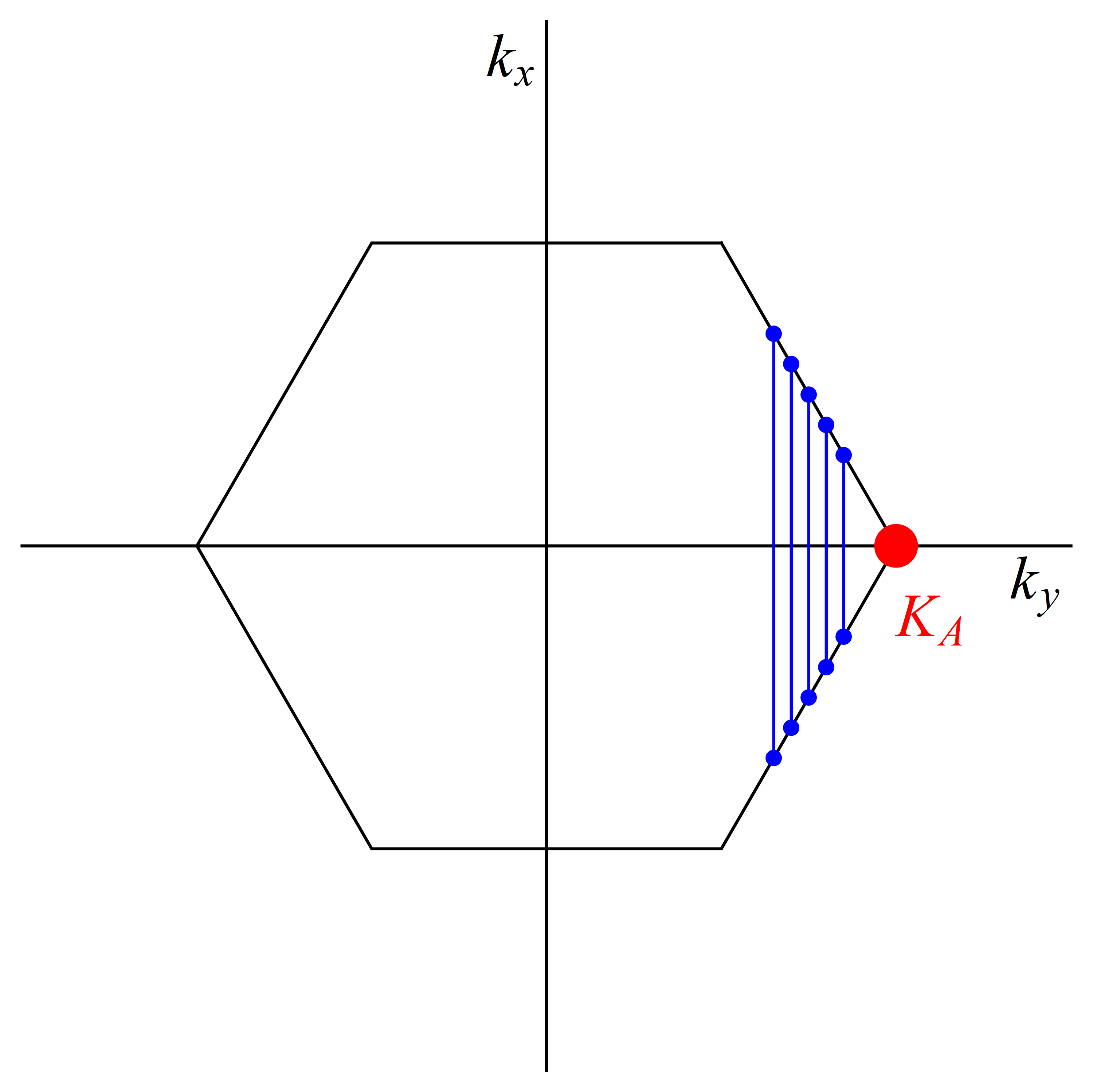
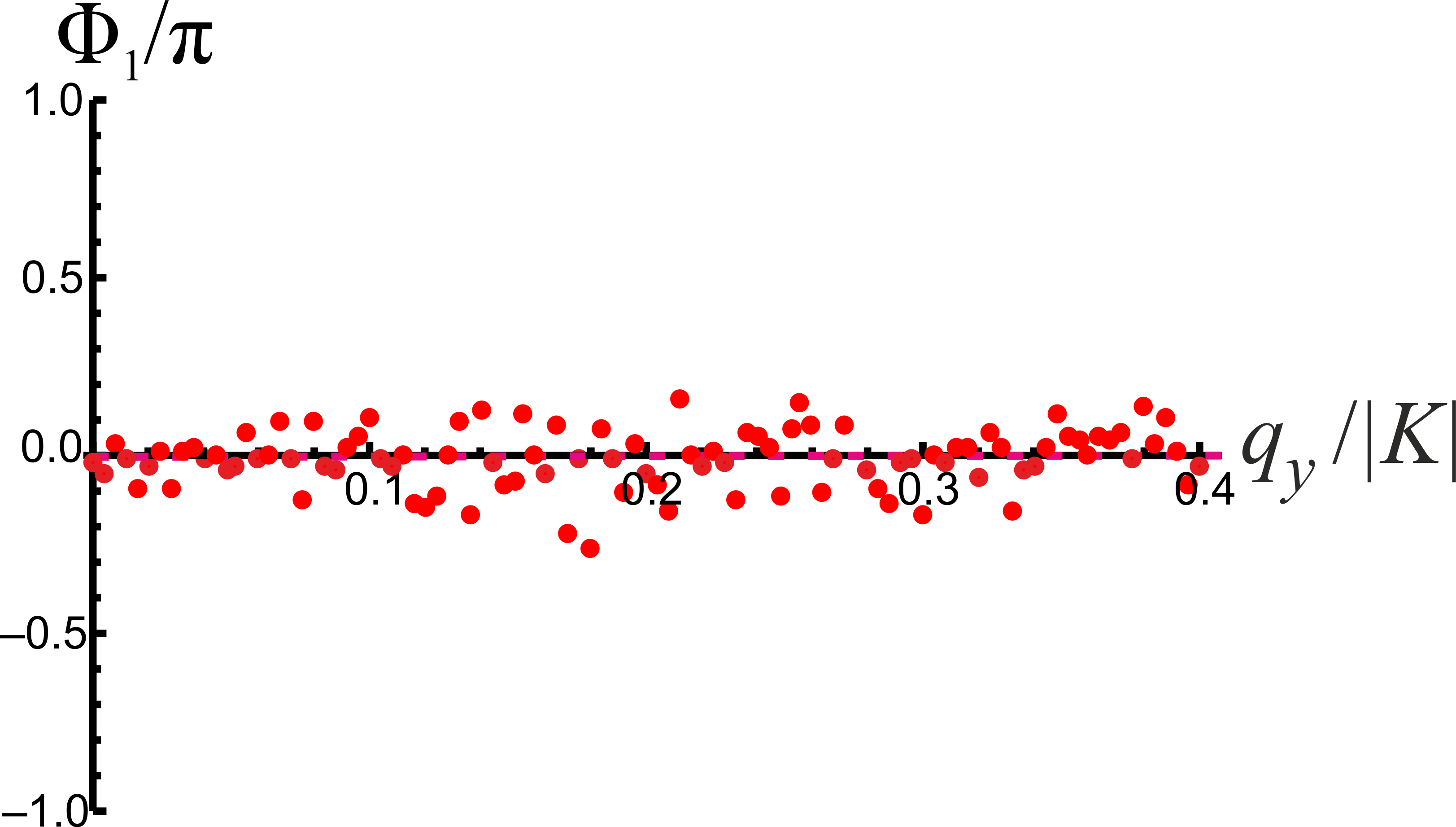
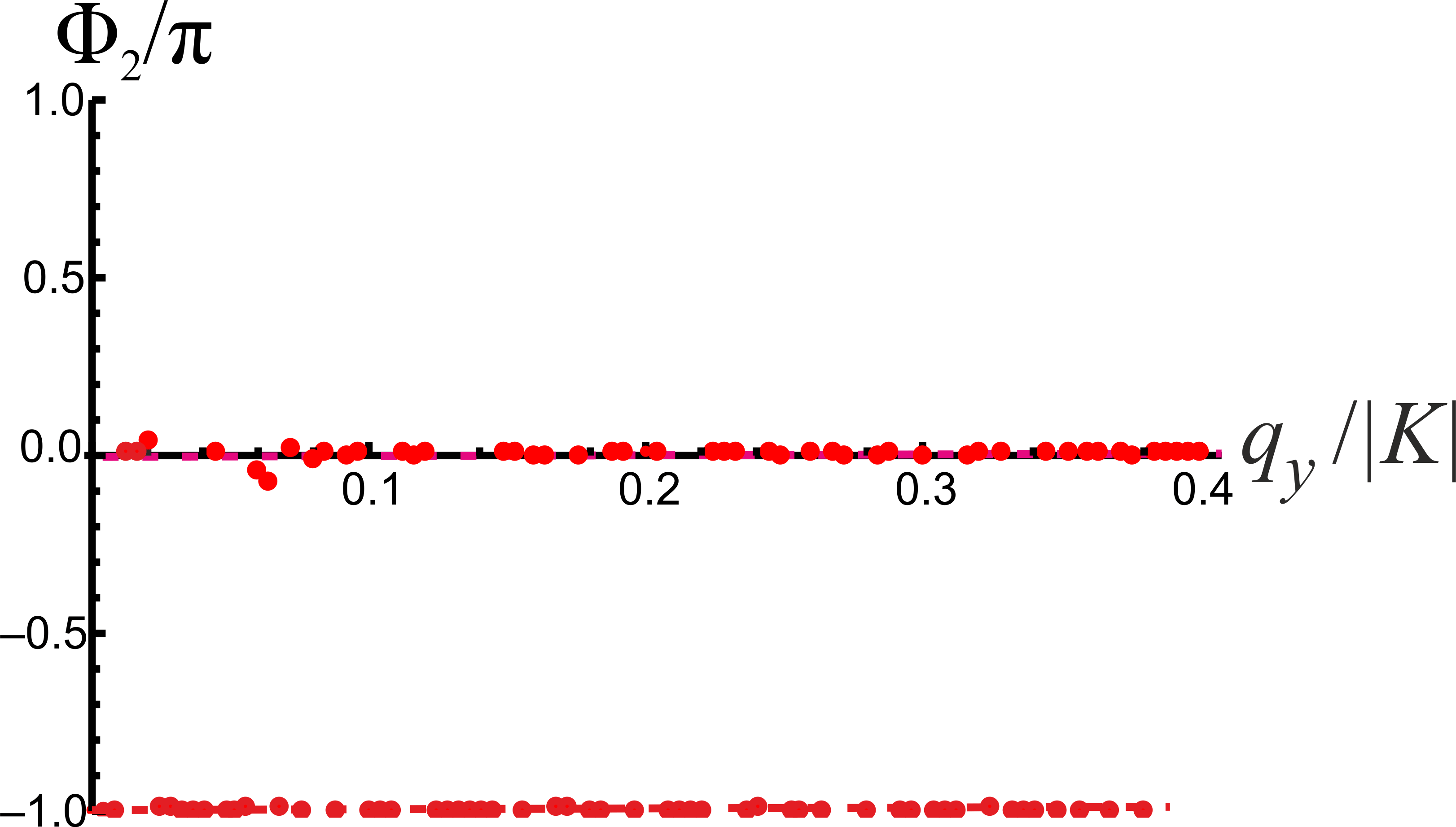
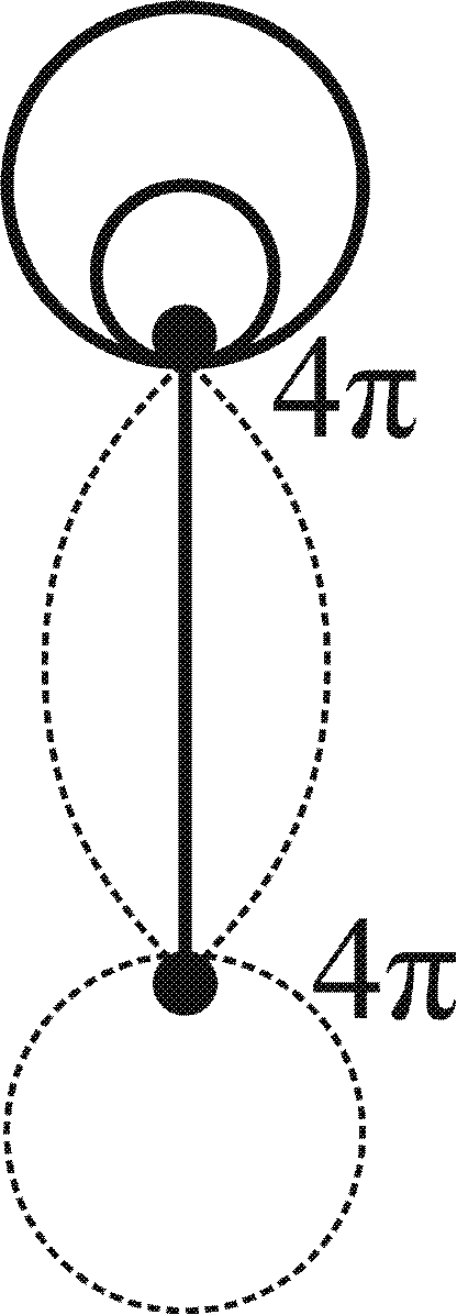
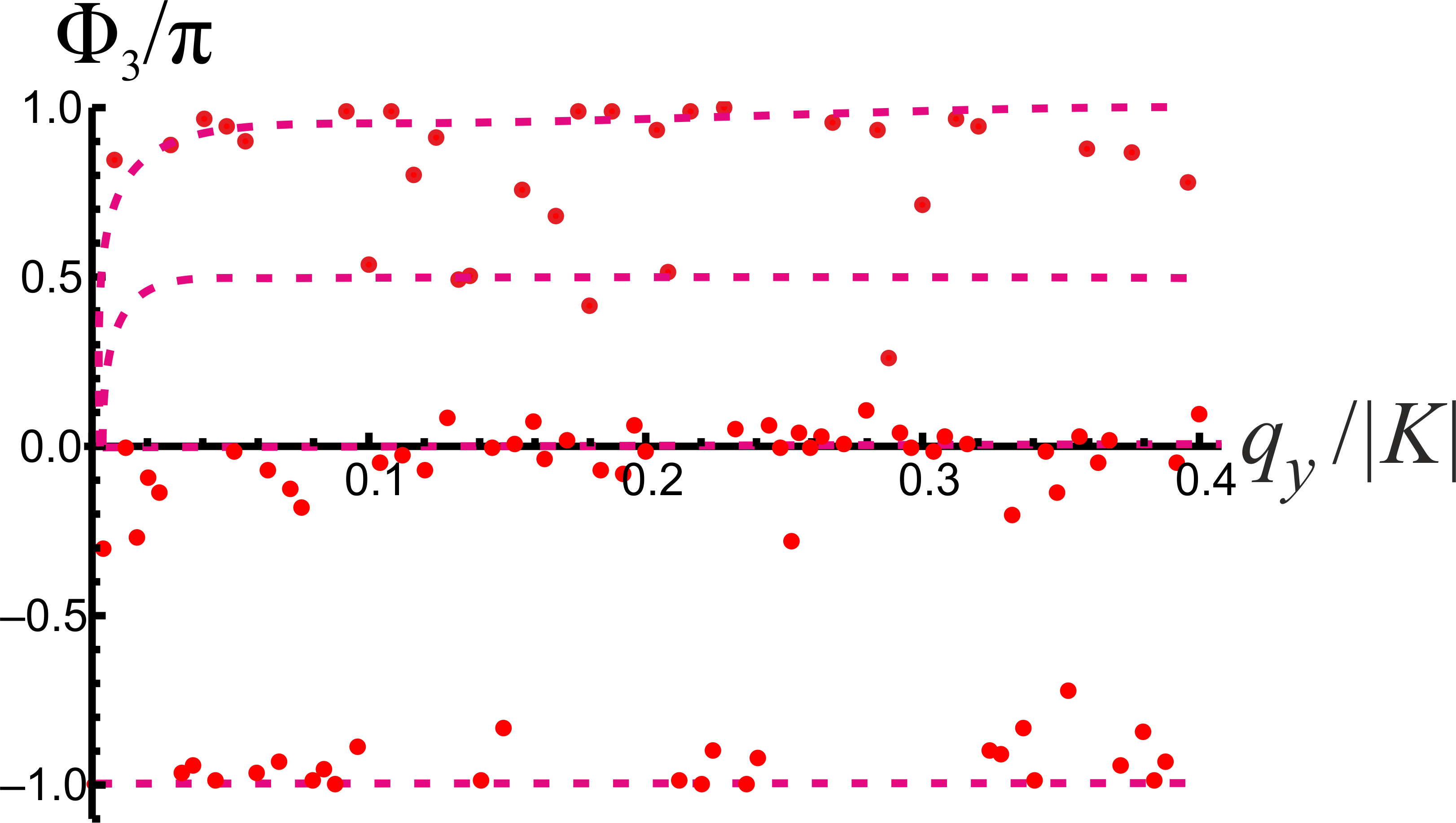
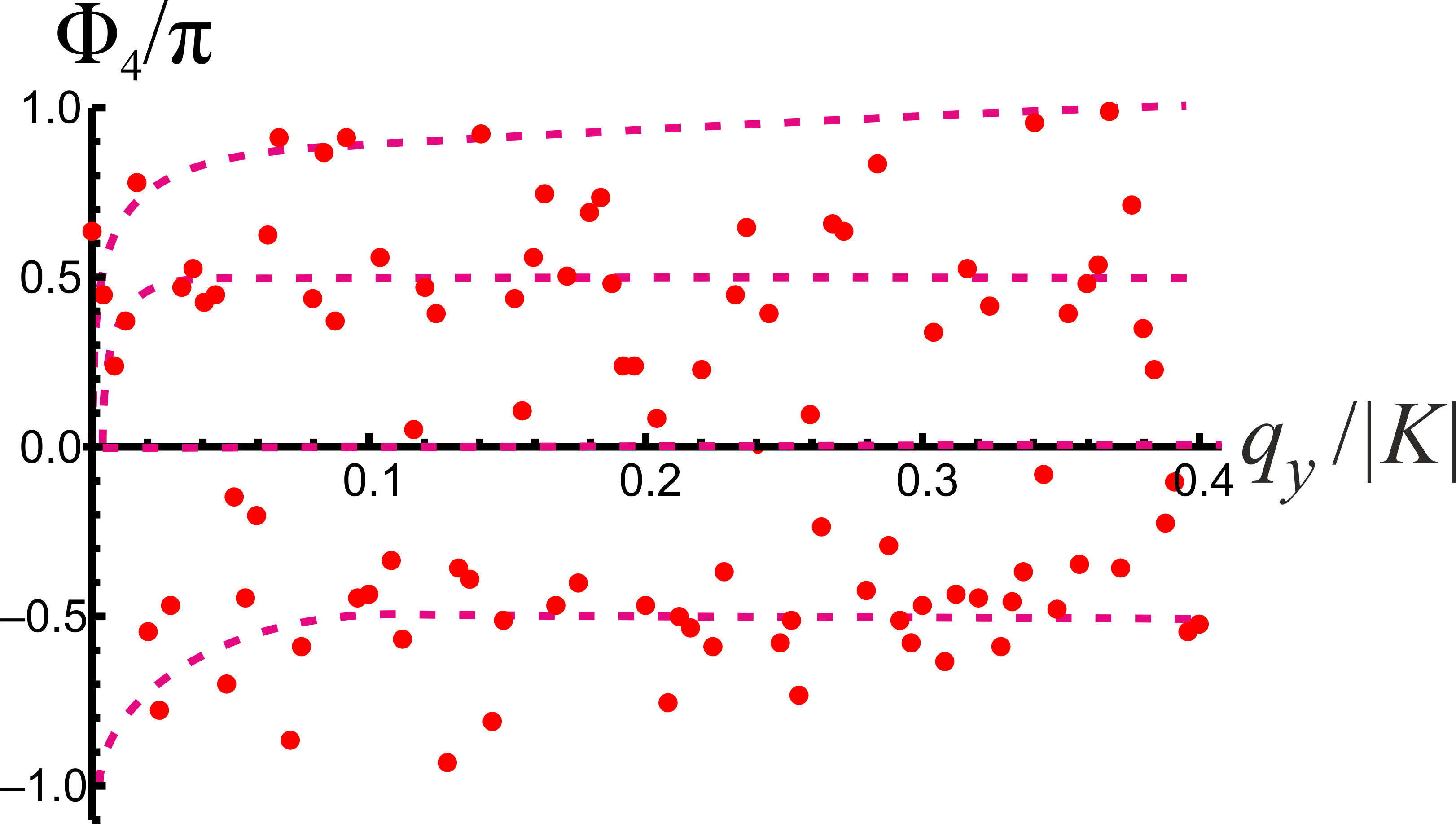
Figure 1: (a) Scheme of Wilson loops for Zak phase calculation. (b) Non-Abelian phases $\Phi_{1},\ldots,\Phi_{4}$ of the Wilson-loop eigenvalues in the units of $\pi$ and (c) sketch of topological defects for quasi-relativistic model of graphene in approximation of zero-values of gauge fields, bypass over each contour in figure (c) gives phase shift value $4\pi$; $\vec{q}=\vec{k}-\vec{K}$.

IV Results and discussion

Simulation of the Zak phases has been performed for three graphene models, the first one is a massless pseudo-Dirac fermion model JPhysB40-2007Semenoff , the second one is our quasi-relativistic graphene model in an approximation of zero gauge field and the third model is the same one but with accounting of non-zero gauge field. The results are presented in Table 1 and figs. 1b, 2a.

(a)                                                                 (c)


                                                                                 
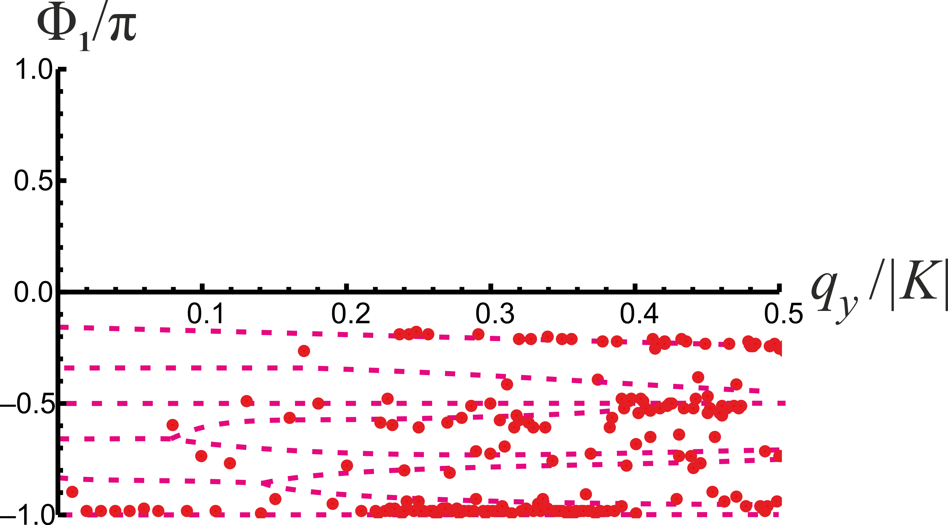
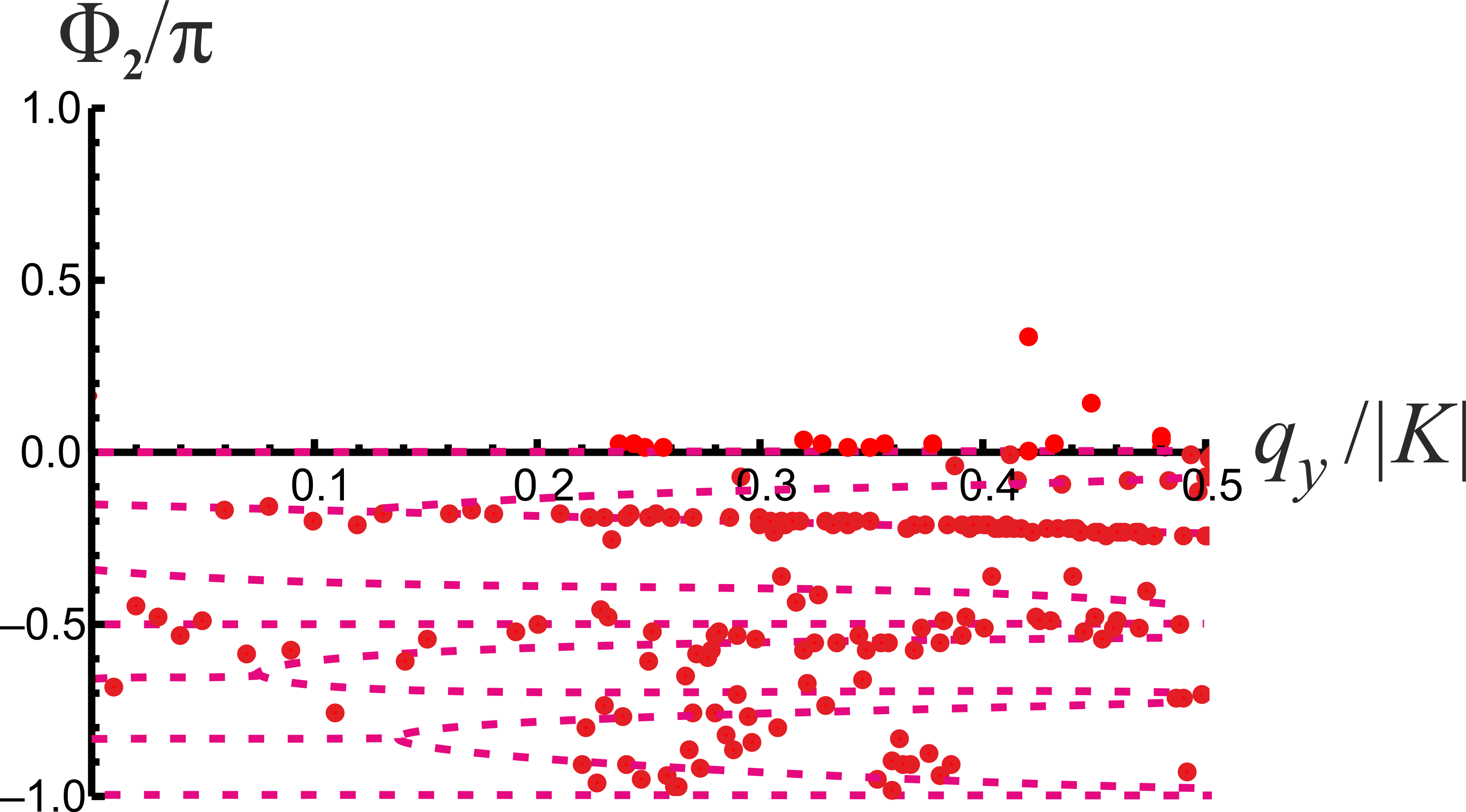
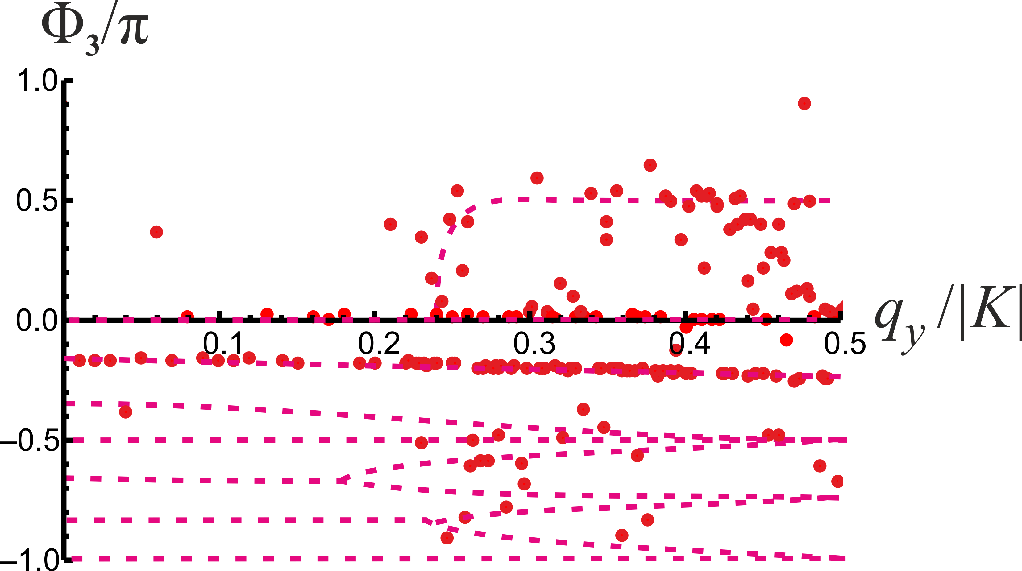
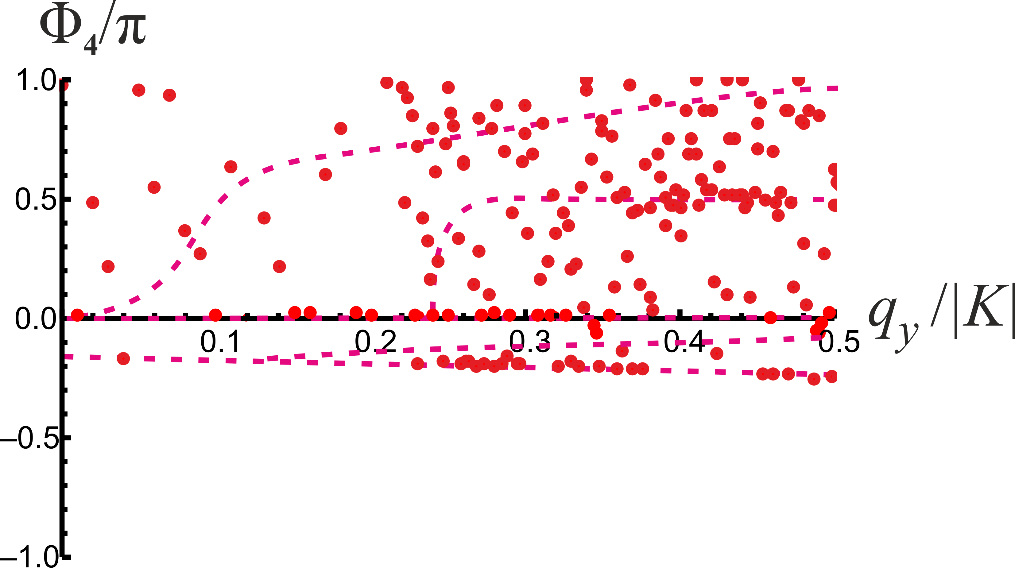
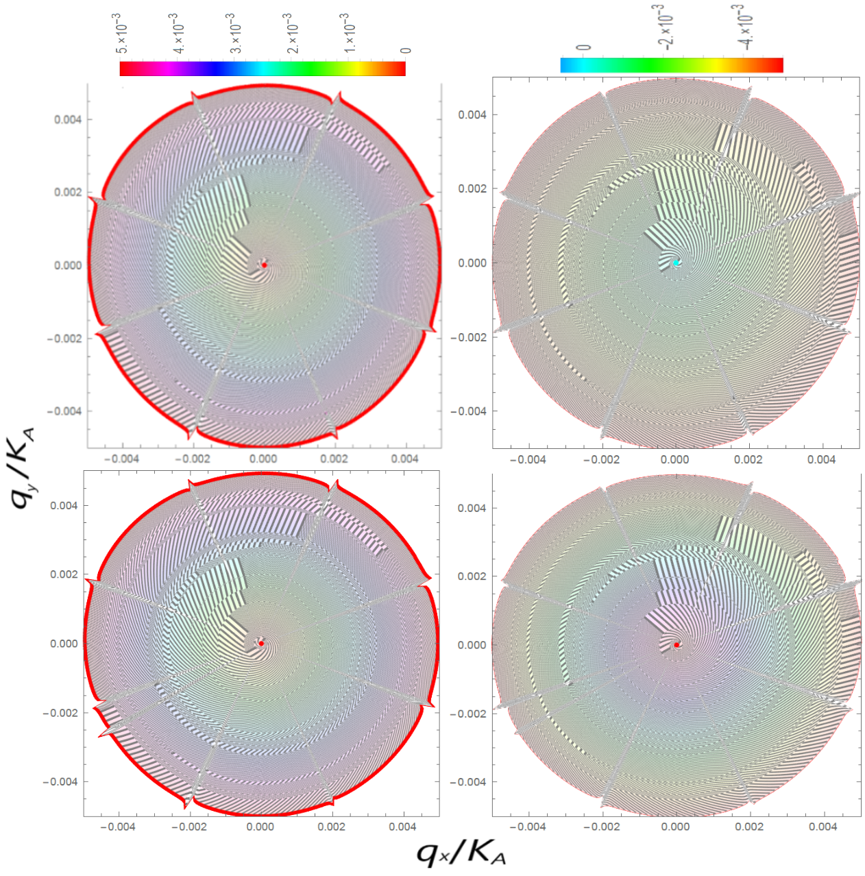
(b)

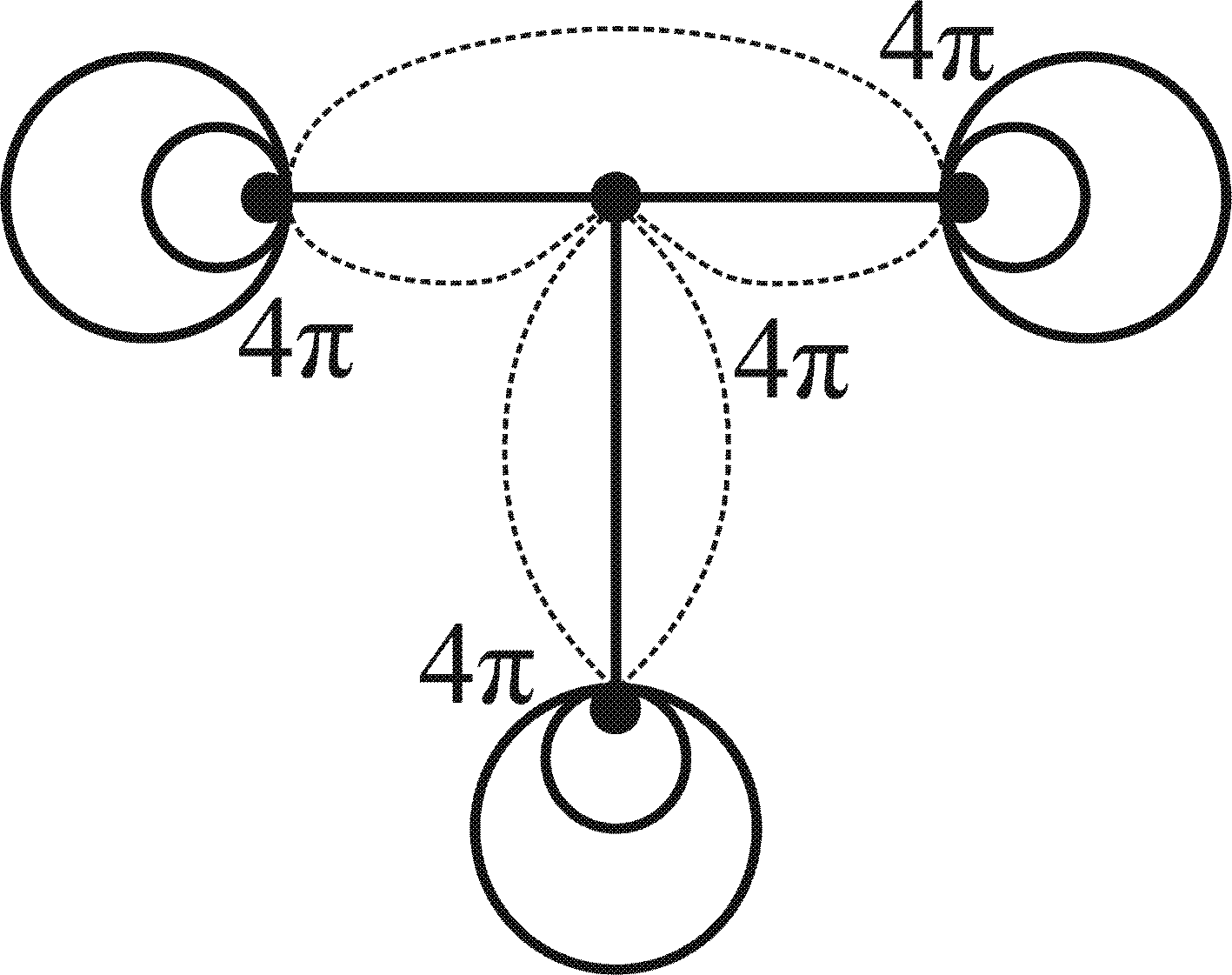
Figure 2: (a) Non-Abelian phases $\Phi_{1},\ldots,\Phi_{4}$ of the Wilson-loop eigenvalues in the units of $\pi$ and (b) sketch of topological defects for quasi-relativistic model of graphene with non-zero gauge field, bypass over each contour in figure (b) gives phase shift value $4\pi$; $\vec{q}=\vec{k}-\vec{K}$. (c) A vortex texture in contour plots of electron (left) and hole (right) bands at the non-zero gauge field, bands have been calculated on momentum scales $q/|K|\sim 0.002$ for non-interacting (up) and interacting (down) electron and hole constituted a Majorana particle.

Up to finite accuracy of the numeric method we get a discrete set of obtained values of phases for considered models. For the massless Dirac model, arguments of the Wilson-loop eigenvalues are equal to $0,\pm\pi$ and are multipliers of $\pi/3$. Hence, due to hexagonal symmetry of the lattice the first model is topologically trivial one.

For the second model, there exist two different sets of the Wilson-loop-arguments eigenvalues, namely, one set $0,\pm\pi$ in the vicinity of the Dirac point $K(K^{\prime})$, the second one $0,\pm\pi/2,\pm\pi$ at sufficiently high values of wavevectors $q_{y}=k_{y}-K_{A,y}$ (see fig. 1b). In the vicinity of $K(K^{\prime})$ the arguments of the Wilson-loop eigenvalues form the same cyclic group $\mathbb{Z}_{2}$, as for the case of the massless pseudo-Dirac model. This testifies on topological non-triviality of the second model. Additional values $\pm\pi/2$ of the Wilson-loop arguments and, respectively, two cyclic groups $\mathbb{Z}_{4}$ with generators $\pi/2$ or $-\pi/2$ are at values of $q_{y}/|K_{A}|$ higher than $0.05$. The observed deformation of the cyclic group $\mathbb{Z}_{2}$ to $\mathbb{Z}_{4}$ is a consequence of the increase in spin-orbit interaction at the high $q_{y}$. The strong spin-orbital coupling lifts the degeneration on pseudospin. Meanwhile Weyl node and antinode emerge. Due to the fact that the cyclic group is $\mathbb{Z}_{4}$, the Weyl node (antinode) should be a double defects (in the form of two singular points). Only in this case, as it is shown in fig. 1c, bypassing the doubled node (antinode) along a contour with a double rotation on an angle $4\pi$ gives the phase shift for the wave function by $2\pi$. Since the Weyl node (antinode), like any quantum fermion state, is a Kramers doublet, then its doubling is a result of splitting spin degeneration owing to the spin-orbital-coupling breaking of time-reversal symmetry but without breaking of electron-hole symmetry. Resulting homotopy group $\mathbb{Z}_{2}\times\mathbb{Z}_{4}$ reveals a broken symmetry for the approximation of the quasi-relativistic model with zero gauge field. Hereafter we show that the broken-symmetry group $\mathbb{Z}_{2}\times\mathbb{Z}_{4}$ recovers to $\mathbb{Z}_{8}$ of the quasi-relativistic model in the approximation of with non-zero gauge field.

As simulation results for the third model demonstrate in fig. 2a, pathes with the topological Zak phase $-\pi/6$ constitute the cyclic groups $\mathbb{Z}_{12}$ in the vicinity of $K(K^{\prime})$ at small momenta $q_{y}$ and additional Majorana Wilson-loop-arguments eigenvalues, multiple to $-\pi/4$ are appeared at high $q_{y}$. These results testify that the quasirelativistic graphene model is topologically nontrivial one in all energy range. A $(-\pi/6)$ rotation is equivalent to a $(-\pi/2)$ rotation due to hexagonal symmetry and, correspondingly, the electron and hole configurations in the momentum space are orthogonal to each other. A schematic representation of this electron-hole configuration in the form of a T-shaped trijunction of four peculiar points (topological defects) is presented in fig. 2b. An atomic chain with two topological defects at the ends implements a Majorana particle. Therefore, the trijunction is formed by three Majorana particles (modes) with flavor, a number of flavors $N=3$. The total angular momentum $\vec{J}$ of such a Majorana-like excitation is equal to $\vec{J}=\sum_{i=1}^{3}\vec{j}_{i}$ with the absolute value $J=3/2$. Here $\vec{j}_{i}$ is angular momentum of $i$-th Majorana particle, $i=1,2,3$. Majorana and antiMajorana states (excitations) with $J=3/2$ differ by the projections $J_{y}=-3/2,-1/2,1/2,3/2$ of the total angular momentum $\vec{J}$. Therefore the Majorana and antiMajorana excitations confined in the Dirac point by hexagonal symmetry are fourth-fold degenerated. The cyclic group $Z_{12}$ existing at small momenta $q$, $q\to 0$ testifies that hexagonal symmetry confines the Majorana mode in the vicinity of the Dirac point owing to small spin-orbital coupling. Simulations discovers eight right- and left-handed vortices on the surfaces of electron and hole bands that one can observes in fig. 2c. We associate each component of the Majorana (anti-Majorana) excitation with the projection $J_{y}$ one of these vortex states of the band structure. Then, the coincidence of the four left-(right-) handed vortices for the fourfold degenerate quasirelativistic graphene model bands at small $q$, $q\to 0$ implies the degeneracy of these vortices. We call these vortex states subreplicas.

Increasing spin-orbit interaction at high $q_{y}$ splits the degeneracy of Majorana and antiMajorana vortex states on $J_{y}$ and, correspondingly, the degeneracy of the subreplicas. The appearance of eight subreplicas is showed in fig. fig3a,b. This octal splitting of conical bands represents a phenomenon of Majorana particles deconfinement. The deconfinement violates the hexagonal symmetry that the high-energetic defects deform the cyclic group $Z_{12}$ with the generator $-\pi/6$ to $Z_{8}$ with the generator $-\pi/4$. Zak phase values, multiple to $\pi/4$, appear at momenta $q_{y}>0.2|K|$ as it is shown in fig. 2a. The deformation is accompanied by subsequent flatting of the bands that the Fermi velocity trends to 0 as figs 3a,b demonstrate. Since the Majorana ”force” (III.26) diverges for the flat bands, four vortices in the T-trijunction are always linked at high energies, but they become asymptotically free in the vicinity of the Dirac points ($q\to 0$). It testifies that the conservation law of topological charge holds.

A configuration of four deconfined vortices is equivalent to a T-shaped trijunction system of three Majorana modes or anti-modes. As it is shown in fig. 2b, the bypass of the T-shaped trijunction over a contour with four turns by an angle of $4\pi$ gives a phase shift for the wave function by $2\pi$, while at bypass of a single vortex defect the wave function acquires the phase $\pi/4$.

The splitting of the Dirac cones by strong spin-orbital coupling into non-coinciding four electron and four hole subreplicas implies the break of electron-hole symmetry. This violation is revealed as an appearance of additional topological Zak phases equal to $\pi/2,\pi$, and correspondingly an additional cyclic group $Z_{4}$ at values of momentum $q_{y}>0.24|K|$. Resonances and antiresonances that are non-invariant with respect to change in sign of the energy band $E$ of the form $E\to-E$ are observed in the band structure (see fig. 3a,b) as a manifestation of broken electron-hole symmetry due to strong spin-orbital coupling. Vortices are created in pairs. Therefore, one can assume that the observed resonances and anti-resonances are respectively the cores (sinks) and anti-core (sources) of the vortices remaining after the destruction of their pair at the spin-orbital coupling. Such topological defects are monopoles and are called Weyl nodes and antinodes. Since the homotopy group is $Z_{4}$, the Weyl nodes (antinodes) in the quasirelativistic graphene model are doubled. Since spin states are Kramers doublets, this doubling can be explained by violation of the symmetry of time reversal, that splits the Kramers degeneracy on spin of Weyl nodes and antinodes. We have also investigated the effect of the interaction between electrons and holes in pairs that the Majorana mass operator $M_{AB}$ ($M_{BA}$) is a dynamical mass due to this interaction. It turns out that this interaction preserves the vortex structure both Majorana and anti Majorana excitation in the vicinity of the Dirac points (see figs. 2c, 3c). The Majorana mass correction to energy hole (up) and electron (down) bands, presented in fig. 3d, is very small, of the order of $10^{-5},10^{-6}$ and is vanishing in $K(K^{\prime})$. Beyond the Dirac points the degree of chirality for one of two Majorana excitations (either Majorana or anti Majorana excitation) changes that the vortex picture in the form of distribution of numerous vortex sleeves changes for only one of the eigenvalues of the operator of dynamical mass $M_{AB}$ ($M_{BA}$) in accord to comparison of the vortex structures calculated with accounting of and without accounting of the interaction in electron hole pair and presented in a contour plots of figs. 2c and 3c,d.

Thus, chiral symmetry of the quasirelativistic graphene model exists not only in the Dirac point, but beyond it. As fig. 3d demonstrates, the mass term leads to the appearance of the center of inversion in band structure. The inversion symmetry excludes the mirror symmetry that the Dirac point is split on the Weyl node and antinode. Besides, in accordance with the comparison of the band structures calculated with accounting and without accounting of interaction in the electron-hole pairs in figs. 3a,b the shift of Weyl nodes and antinodes into the region of higher energies testifies that the mass-term shifts the location of Weyl nodes and antinodes into the region of higher energies and accordingly the Majorana-like modes can exist without mixing with the nodes.

(a)                                           (c)
               
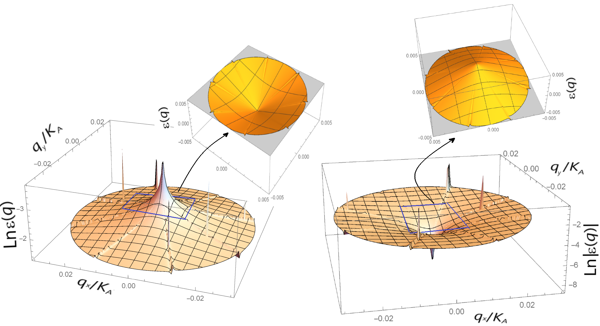
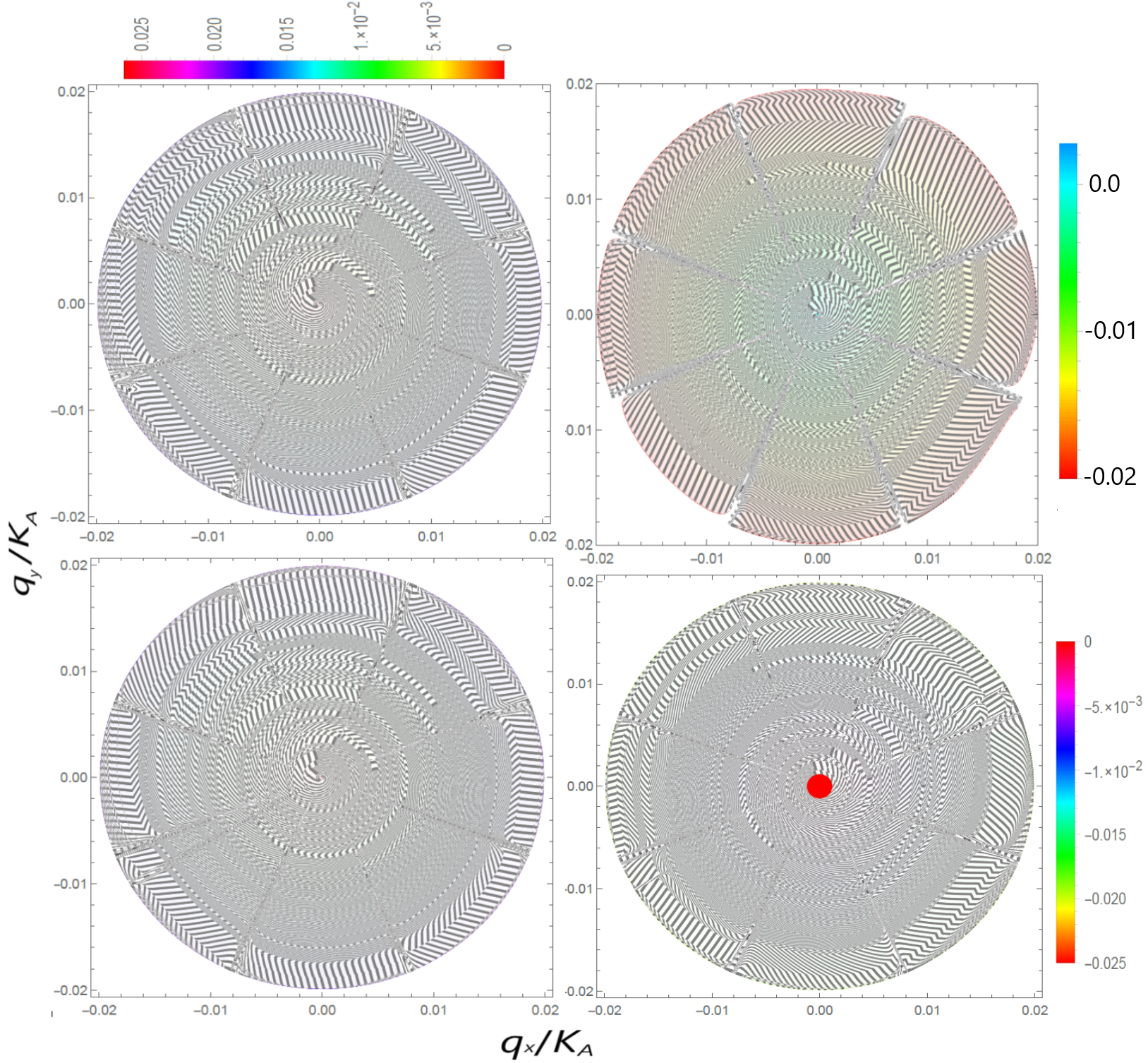
                          (b)                                           (d)
           

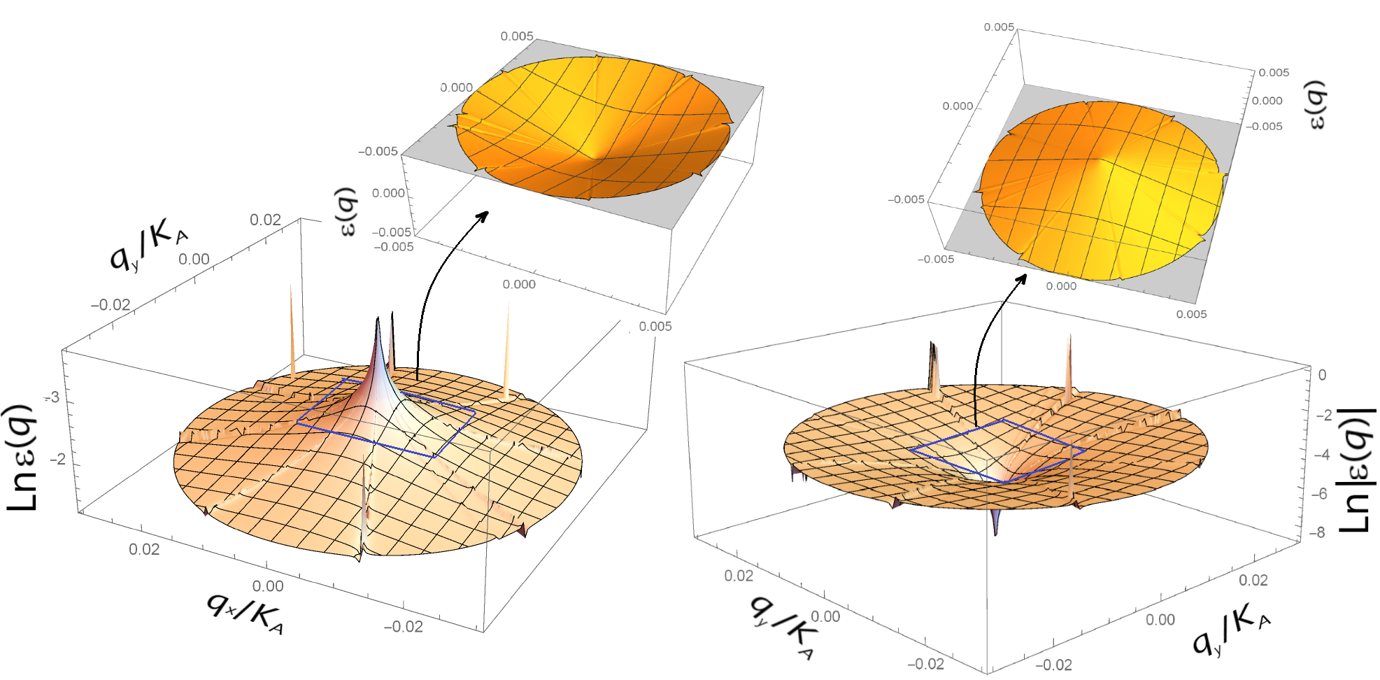
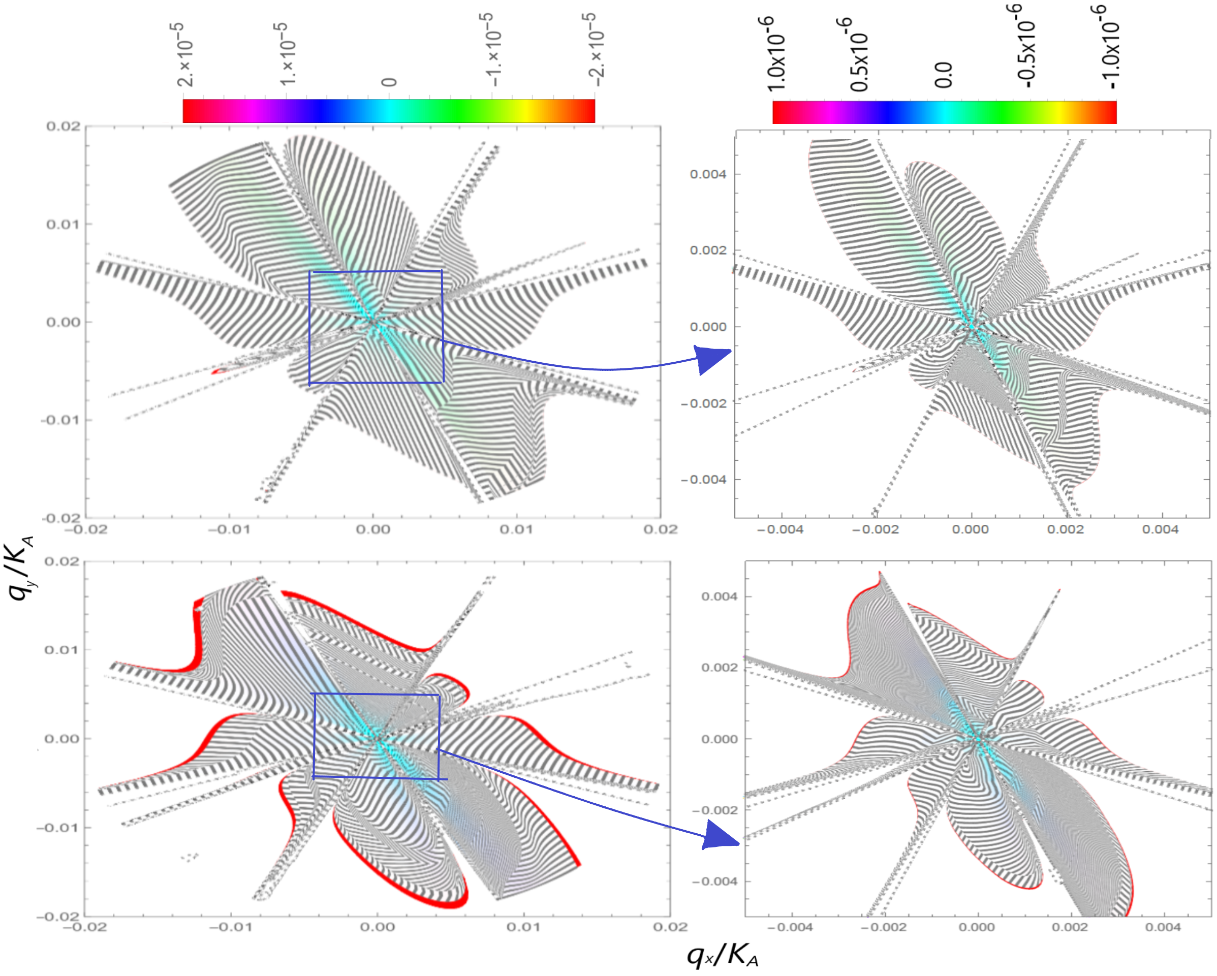
Figure 3: Band structure with account of (a) and without account of (b) interaction in electron-hole pair on momentum scale $q/|K|\sim 0.02$ for quasi-relativistic model of graphene with non-zero gauge field. (c) Vortex textures in contour plots of electron (left) and hole (right) bands at the non-zero gauge field, bands have been calculated on momentum scales $q/|K|\sim 0.01$ for non-interacting (up) and interacting (down) electron and hole constituted a Majorana particle. (d) Mass correction to the energy hole (up) and electron (down) bands.

V Conclusion

Let us summarize our findings. Simulations of non-Abelian Zak phases and band structure of the quasi-relativistic graphene model have been performed within two approximations of zero- and non-zero values of gauge fields. It has been found that in the approximation of zero gauge field, Zak phases discrete set testifies that the Dirac point is topologically trivial one. Outside of the valleys the set is the cyclic group $\mathbf{Z}_{2}\times\mathbf{Z}_{4}$. This cyclic group testifies that the electron-hole degeneration is broken leading to emergence of double Weyl nodes and antinodes. The approximation of non-zero gauge fields turns out to be topologically non-trivial at all energy scale. In this case the Zak phase set forms a cyclic group $\mathbf{Z}_{12}$ which at sufficiently high momenta is deformed into $\mathbf{Z}_{8}$. It implies that topological vortex defects observed in contour plots of graphene band structure are confined by hexagonal symmetry in the Dirac point. Increasing spin-orbit interaction at high momenta leads to deconfinement of Majorana modes. The deconfinement violates the hexagonal symmetry that the high-energetic defects deform the cyclic group $\mathbf{Z}_{12}$ to $\mathbf{Z}_{8}$. The following effects of the Majorana mass term on the graphene band structure have been discovered. The first one is the emergence of inverse symmetry at ”switching on” of the mass term. The second one is a mass-term shifting of Weyl nodes and antinodes into the region of higher momenta. It signifies that after the deconfinement pure Majorana-like state can exist in sufficiently large energy region.

References

- (1) H.-Zh. Lu, Sh.-Q. Shen. Front. Phys. 12(3), 127201 (2017).
- (2) Gu. Bian et al. Nature Communications. 7, 10556 (2016)
- (3) L. Muechler et al. Phys. Rev.X. 6, 041069 (2016).
- (4) Jin-Lian Lu et al. Chin. Phys. Lett. Vol. 34, No. 5 (2017) 057302
- (5) P. San-Jose et al. Phys. Rev. X. 5, 041042 (2015).
- (6) V.K. Sangwan, M.C. Hersam. Annual Review of Physical Chemistry. Vol. 69, 299-325 (2018).
- (7) A.Y. Kitaev. Physics Uspekhi. 44(Suppl.), 131-136 (2001).
- (8) G.W. Semenoff, P. Sodano. J.Phys.B. 40, 1479-1488 (2007).
- (9) C.W.J. Beenakker. Annu. Rev. Condens. Matt. Phys. 4, 113-136 (2013).
- (10) Ya.Peng et al. PRL 115, 266804 (2015).
- (11) B. van Heck et al. New J. Phys. 14, 035019 (2012).
- (12) L. Fu, C.L. Kane. Phys. Rev. Lett. 100, 096407 (2008).
- (13) M.-L. Ge, L.-W. Yu. Int. J. Mod. Phys. B 28, 1450089 (2014). DOI: 10.1142/S0217979214500891
- (14) C. Nayak, F. Wilczek. Nucl. Phys. B 479, 529 (1996).
- (15) D. Ivanov. Phys. Rev. Lett. 86, 268 (2001).
- (16) A.Y. Kitaev. Ann. Phys. 303, 2 (2003).
- (17) C. Nayak et al. Rev. Mod. Phys. 80, 1083 (2008).
- (18) F. von Oppen, Ya. Peng, F. Pientka. Topological superconducting phases in one dimension. (Oxford University Press, Oxford, 2015).
- (19) H.V. Grushevskaya, G.G. Krylov. Symmetry. 8,60 (2016).
- (20) H.V. Grushevskaya, G.G. Krylov. Int. J. Nonlin. Phenom. in Complex Sys. Vol. 20, 153 -169 (2017).
- (21) H.V. Grushevskaya, G.G. Krylov. In: Graphene Science Handbook: Electrical and Optical Properties. Vol. 3. Chapter 9. Eds. M. Aliofkhazraei et al.(Taylor and Francis Group, CRC Press, USA, UK, 2016). Pp.117-132.
- (22) H.V. Grushevskaya, G.G. Krylov. Semiconductors. Vol. 52. no. 14, 1879-1881 (2018).
- (23) Y. Cao et al. Nature. 556, 43 (2018).
- (24) R. Bistritzer, A.H. MacDonald. PNAS. 108, 12233 (2011).
- (25) V.A. Fock. Foundations of quantum mechanics. (Science Publishing Company, Moscow, 1976) (in Russian).
- (26) H.V. Grushevskaya, G. Krylov. J. Nonlin. Phenom. in Complex Sys. 18, no. 2, 266-283 (2015).
- (27) H.V. Grushevskaya et al. Int. J. Nonlin. Phenom. in Complex Sys. 18, no. 1, 81-98 (2015).
- (28) J. Zak, Phys. Rev. Lett. 62 2747 (1989)
- (29) A. Alexandradinata et al. Phys. Rev. B89, 155114 (2014).