Cosmological implications of a modified galaxy cluster pressure profile using the Planck tSZ power spectrum

Abstract

The mean pressure profile of the cluster population is a key element in cosmological analyses based on surveys of galaxy clusters observed through the Sunyaev-Zel’dovich (SZ) effect. A variation of both the shape and the amplitude of this profile could explain part of the discrepancy currently observed between the cosmological constraints obtained from the analyses of the CMB primary anisotropies and those from cluster abundance in SZ surveys for a fixed mass bias parameter. We study the cosmological implications of a modification of the mean pressure profile through the analysis of the SZ power spectrum measured by Planck. We define two mean pressure profiles on either side of the one obtained from the observation of nearby clusters by Planck. The parameters of these profiles are chosen to ensure their compatibility with the distributions of pressure and gas mass fraction profiles observed at low redshift. We find significant differences between the cosmological parameters obtained by using these two profiles to fit the Planck SZ power spectrum and those found in previous analyses. We conclude that a ${\sim}15\%$ decrease of the amplitude of the mean normalized pressure profile is sufficient to alleviate the discrepancy observed between the constraints of $\sigma_{8}$ and $\Omega_{m}$ from the CMB and cluster analyses.

1 Introduction

The abundance of galaxy clusters as a function of mass and redshift has been shown to be a powerful cosmological probe as it is both sensitive to the statistical properties of the matter distribution at the end of the inflation and to the growth of structures across the whole history of the universe (Voit , 2005). The thermal Sunyaev-Zel’dovich (tSZ) effect is an excellent observable to measure the distribution of galaxy clusters up to very high redshift (Bocquet et al., 2019). The calibration of both the mean normalized pressure profile of the cluster population and the scaling relation that relates the tSZ observable and cluster mass is fundamental to establishing accurate cosmological constraints from the analysis of tSZ surveys. The analysis of the tSZ angular power spectrum measured by Planck (Planck Collaboration , 2016) have enabled estimating the amplitude of the linear matter power spectrum at a scale of $8h^{-1}$Mpc, $\sigma_{8}$, and the total matter density of the universe $\Omega_{m}$. However, these cosmological constraints are in tension with the ones obtained from the analysis of the power spectrum of the CMB temperature anisotropies (Planck Collaboration , 2016b).
A significant amount of research has been made to show that this tension could be due to a limit in the $\Lambda$CDM model or to a biased estimation of the mass of galaxy clusters. Part of this discrepancy may also be due to a mass and redshift evolution of the mean normalized pressure profile. Indeed, the ones currently used in tSZ cosmological analyses have been estimated using cluster samples at low redshift and high mass (Arnaud et al., 2010; Planck Collaboration et al., 2013). However, deviations from the self-similar hypothesis may lead to significant differences between these profiles and the true mean normalized pressure profile of the cluster population. One of the goals of the NIKA2 (Adam et al., 2018) tSZ large program is to analyze the potential redshift evolution of the mean normalized pressure profile (Perotto et al., 2018). In this paper, we study the impact of a modification of the mean normalized pressure profile of the cluster population on the constraints of the $\sigma_{8}$ and $\Omega_{m}$ parameters derived from the analysis of the tSZ power spectrum measured by Planck (Planck Collaboration , 2016).

2 Cosmology from the tSZ power spectrum

2.1 Model of the tSZ power spectrum

We model the tSZ power spectrum using only the one-halo component as the two-halo term has been shown to be negligible given the precision of the current tSZ measurements (Komatsu & Kitayama , 1999). It is given at a multipole $\ell$ by:

$$C_{\ell}^{tSZ}=\int\frac{d^{2}V}{dzd\Omega}\,dz\int\frac{dn}{dM_{500}}\,\left|\frac{4\pi R_{500}}{\ell_{500}^{2}}\frac{\sigma_{T}}{m_{e}c^{2}}\,P_{500}\,I_{\mathbb{P}}(\ell_{500})\right|^{2}\,dM_{500}$$ (1)

where $m_{e}$ is the electron mass, $c$ the speed of light, and $\sigma_{\mathrm{T}}$ the Thomson scattering cross section. The characteristic radius $R_{500}$ is the upper integration limit at which the mean cluster density is $500$ times the critical density of the universe. The mass function $dn/dM_{500}$ gives the expected halo number density for a cluster mass $M_{500}$. Its amplitude highly depends on the value of the $\sigma_{8}$ and $\Omega_{m}$ parameters. The tSZ power spectrum also slightly depends on the Hubble parameter $H_{0}$ through the comoving volume element $d^{2}V/dzd\Omega$. A key element in this model is the $I_{\mathbb{P}}(\ell_{500})$ function giving the normalized two dimensional Fourier transform of the mean pressure profile. It is given under the Limber’s approximation by (Komatsu & Seljak , 2002):

$$I_{\mathbb{P}}=\int x^{2}\frac{\mathrm{sin}(\ell x/\ell_{500})}{\ell x/\ell_{500}}\mathbb{P}(x)\,dx$$ (2)

where $x=r/R_{500}$, $\ell_{500}\equiv D_{A}/R_{500}$, $D_{A}$ is the angular diameter distance, and $\mathbb{P}(x)$ is the mean normalized pressure profile of the cluster population. We model this profile using a generalized Navarro-Frenk-White model (gNFW, Nagai et al., 2007):

$$\mathbb{P}(x)=\frac{P_{0}}{(c_{500}x)^{\gamma}[1+(c_{500}x)^{\alpha}]^{(\beta-\gamma)/\alpha}}$$ (3)

This profile is scaled by the $P_{500}$ parameter in Eq. (1) to account for the mass dependence of the cluster pressure content. It has been shown by Bolliet et al. (Bolliet et al., 2018) that the amplitude of the power spectrum of the tSZ effect scales with the combined parameter

$$F=\sigma_{8}\,(\Omega_{m}/B)^{0.40}\,h^{-0.21}$$ (4)

where $h=H_{0}/[100\leavevmode\nobreak\ \mathrm{km/s/Mpc}]$ and $B=1/(1-b)$ is the hydrostatic bias that links the true mass $M_{500}$ to the one given under the assumption of hydrostatic equilibrium $M_{500}^{\mathrm{HSE}}=(1-b)M_{500}$. In the following, we aim at quantifying the implications of a modification of the profile given in Eq. (3) on the cosmological constraints obtained by the analysis of the Planck tSZ power spectrum using the model defined by Eq. (1).

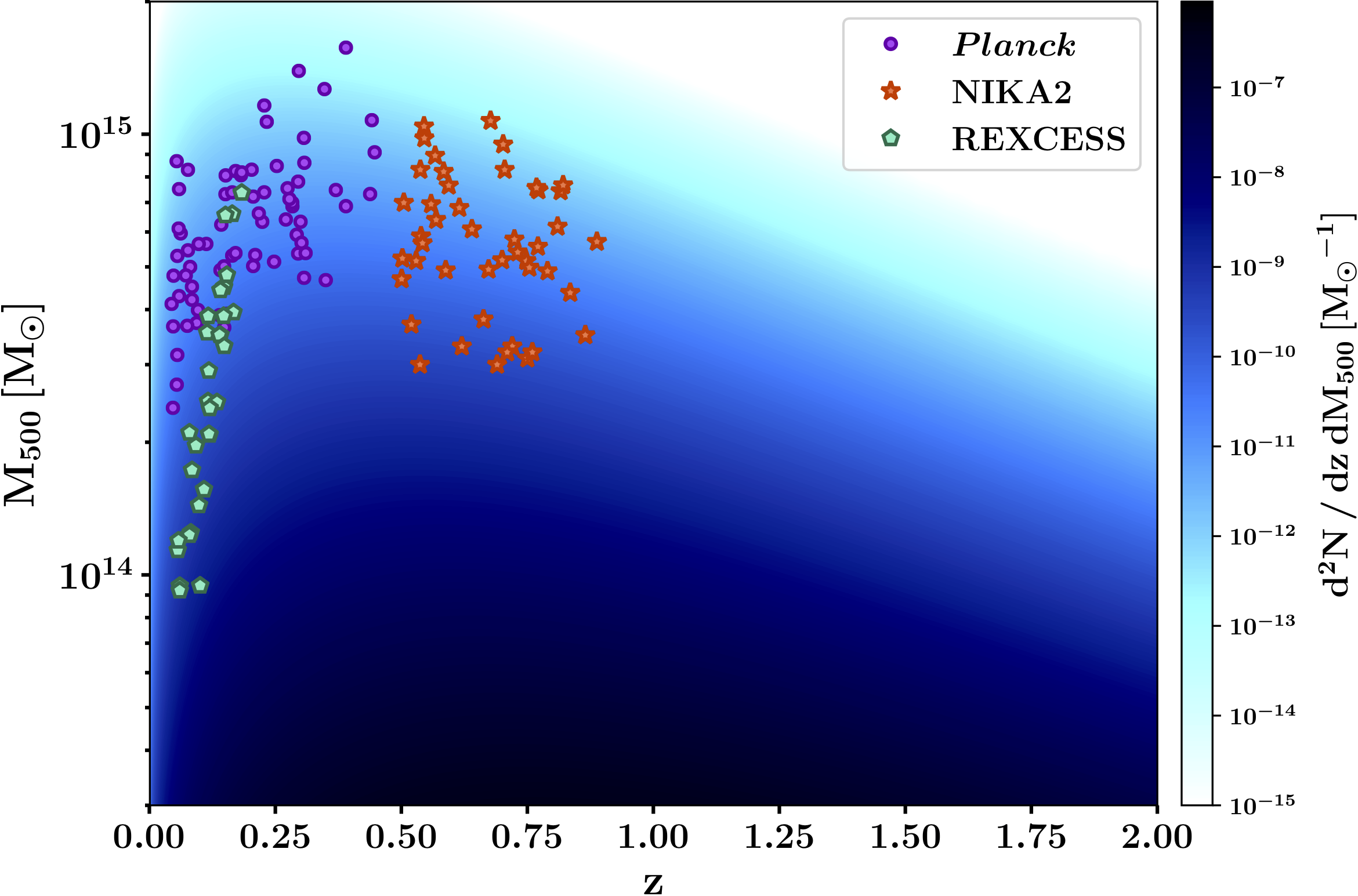
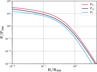
Figure 1: Left: Cluster abundance as a function of mass and redshift (shades of blue). We also show the distributions of the 62 Planck clusters (purple), the REXCESS (green), and NIKA2 (orange) samples. Right: Mean normalized pressure profiles considered in the analysis of the Planck tSZ power spectrum. The profile obtained by Planck is shown in black (Planck Collaboration et al., 2013). The definition of the blue and red profiles is described in Sect. 2.2 (Ruppin et al., 2019).

2.2 Selection of the mean normalized pressure profile

The blue gradient in the left panel of Fig. 1 shows the expected number of clusters per unit of mass and redshift assuming the cosmological parameters given in Planck Collaboration et al. (2018). The low redshift ($z<0.5$) cluster samples REXCESS (Pratt et al., 2009) (green symbols) and Planck (Planck Collaboration et al., 2013) (purple dots) have been considered to establish the most widely used normalized pressure profiles in cosmological analyses. However, the dominant contribution to the tSZ power spectrum comes from the sum of the tSZ signal of low-mass halos at $z\gtrsim 0.3$ because their abundance is ${\sim}3$ times higher than the well-known massive clusters at low redshift (Planck Collaboration , 2016). If cluster self-similarity is not verified across the whole mass-redshift plane, the true mean normalized pressure profile of the cluster population will be different from the ones estimated at low redshift. The cluster sample of the NIKA2 SZ large program (Perotto et al., 2018) (orange stars) has been defined in order to probe a potential redshift evolution of the mean pressure profile.
It is necessary to estimate the impact of a modification of this profile on the estimation of the $\sigma_{8}$ and $\Omega_{m}$ cosmological parameters. We show in the right panel of Fig. 1 the two mean pressure profiles (blue and red lines) that we have defined on either side of the one obtained from the analysis of the 62 nearby clusters in the Planck sample (black line). We have used the gNFW parametric model given by Eq. (3) to define these profiles. Their corresponding parameters have been set such that the profiles are compatible with the distribution of normalized pressure profiles obtained by Planck (Planck Collaboration et al., 2013) given its intrinsic scatter and that the corresponding gas mass fraction is compatible with the observed values at low redshift Planck Collaboration et al. (2013); Eckert et al. (2013, 2019). We estimate the gas mass fraction profile for a given pressure profile by assuming that the cluster mass profiles are given by a Navarro-Frenk-White (NFW) model (Navarro et al., 1997). We explain this procedure in detail in (Ruppin et al., 2019). The two pressure profiles defined with this procedure are called $P_{l}$ and $P_{h}$, whereas the Planck pressure profile is named $P_{m}$ in the following.

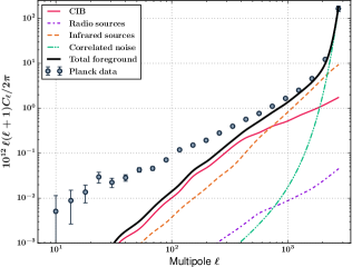
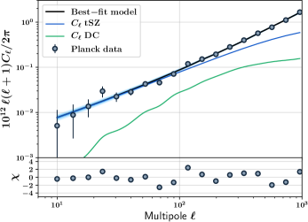
Figure 2: Left: Planck tSZ angular power spectrum measured from the sky $y$-map (Planck Collaboration , 2016) (grey points). The power spectra of the contaminants to the tSZ signal are given by the colored lines and their sum is shown as a black line. Right: Best-fit model of the Planck tSZ power spectrum (black line). The blue line shows the contribution from the tSZ signal to the total power spectrum and the green line is the one due to the detected clusters in the Planck catalog (Planck Collaboration , 2016). The lower panel shows the significance of the residuals after the best-fit model subtraction to the data (Ruppin et al., 2019).

3 Analysis of the Planck tSZ power spectrum

The power spectrum $C_{\ell}^{\mathrm{map}}$ of the Planck map of the tSZ effect (Planck Collaboration , 2016) is represented by the grey points in the left panel of Fig. 2. The error bars $\Delta C_{\ell}^{\mathrm{map}}$ associated with each bin in the power spectrum have been estimated using the cross-power spectra between the sky maps obtained by different detectors of the Planck satellite. All the contaminants to the tSZ signal are not completely excluded by the component separation analysis used to obtain the Planck map of the tSZ effect. The cosmic infrared background (CIB), unresolved infrared sources and radio sources induce significant residuals in the power spectrum. Spatially correlated instrumental noise also induces a significant increase in the power spectrum amplitude in the last multipole bins. Therefore, we model the total power spectrum by the following sum of components:

$$C_{\ell}^{\mathrm{map}}=C_{\ell}^{tSZ}+A_{\mathrm{CIB}}\hat{C}_{\ell}^{\mathrm{CIB}}+A_{\mathrm{IR}}\hat{C}_{\ell}^{\mathrm{IR}}+A_{\mathrm{RS}}\hat{C}_{\ell}^{\mathrm{RS}}+A_{\mathrm{CN}}\hat{C}_{\ell}^{\mathrm{CN}}$$ (5)

where the $\hat{C}_{\ell}^{i}$ are the power spectra of the $i^{th}$ component and $A_{i}$ their corresponding amplitudes. Tabulated models established by the Planck collaboration (Planck Collaboration , 2016) for the power spectrum of the radio sources (RS), infrared sources (IR), CIB, and correlated noise (CN) have been used throughout this analysis. They are represented by colored lines in the left panel of Fig. 2 and their sum is shown as a black line. The dominant contribution to the power spectrum at multipoles $\ell\gtrsim 1000$ comes from these contaminants. Therefore, we choose to discard the bins with marginal information on the tSZ power spectrum and fit $C_{\ell}^{\mathrm{map}}$ up to the multipole bin $\ell=959.5$ to optimize the computation time in our analysis.

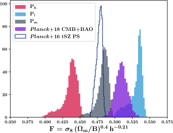
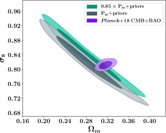
Figure 3: Left: Distributions of $F$ obtained at the end of the MCMC analyses based on the $P_{h}$ (red), $P_{m}$ (grey), and $P_{l}$ (blue) profiles. The distribution estimated by the Planck collaboration is represented by a dark blue line. The distribution obtained from the Planck analysis of the CMB primary anisotropies is also shown in purple. Right: Cosmological constraints obtained on $\sigma_{8}$ and $\Omega_{m}$ using the $P_{m}$ profile (grey) and the $P_{m}$ profile scaled down by 15% (green) for an hydrostatic bias prior of $b=0.20\pm 0.01$. The Planck CMB contours are also shown (purple) (Ruppin et al., 2019).

The three normalized pressure profiles defined in Sect. 2.2 are used in a MCMC analysis to fit the Planck power spectrum $C_{\ell}^{\mathrm{map}}$ (Planck Collaboration , 2016). The free parameters in the analysis are $F$, $\Omega_{m}$, $b$, $h$, $A_{\mathrm{CIB}}$, $A_{\mathrm{IR}}$ and $A_{\mathrm{RS}}$. We fix the value of the amplitude of the power spectrum of the correlated noise to the one of $C_{\ell}^{\mathrm{map}}$ measured in the bin at $\ell=2742$. We use Eq. (1) and (5) at each step of the analysis to compute the total power spectrum $\hat{C}_{\ell}^{\mathrm{tot}}$ given the considered cosmological model and pressure profile. This power spectrum is then compared with the Planck power spectrum in the 18 bins at $\ell<1000$ through the Gaussian likelihood function $\mathcal{L}$ defined by:

$$-2\mathrm{ln}\,\mathcal{L}=\sum_{\ell}\left[\frac{C_{\ell}^{\mathrm{map}}-\hat{C}_{\ell}^{\mathrm{tot}}}{\Delta C_{\ell}^{\mathrm{map}}}\right]^{2}$$ (6)

We use uniform priors to ensure that all the parameters stay positive and that the hydrostatic bias value is such that $0<b<0.4$. Furthermore, we use a Gaussian prior on the Hubble parameter $h=0.67\pm 0.03$ given the latest results obtained by the Planck CMB analysis (Planck Collaboration et al., 2018). After the convergence of the chains and the burn-in cut-off, the remaining samples are used to estimate the marginalized probability densities associated with each parameter. The best-fit power spectrum model obtained at the end of the analysis based on the $P_{m}$ profile is represented by a black line in the right panel of Fig. 2. As shown in the lower panel the statistical significance of the residuals computed after subtracting the best fit model to the measured power spectrum is smaller than $3\sigma$ at each multipole. The same statistical accuracy is reached at the end of the analyses based on the $P_{l}$ and $P_{h}$ profiles.

4 Implications of a modification of the mean pressure profile

The posterior distributions of the $F$-parameter are shown in Fig. 3 for the profiles $P_{h}$ (red), $P_{m}$ (grey) and $P_{l}$ (blue). We compare the distribution of $F$ obtained for the $P_{m}$ profile with the one estimated from the analysis of the tSZ power spectrum performed by the Planck collaboration (Planck Collaboration , 2016) based on the same profile (dark blue line) and find that they are both fully compatible. The mean values of the distributions of the $F$-parameter associated with the $P_{h}$ and $P_{l}$ are significantly different from the one found using the $P_{m}$ profile. This shows that the mean normalized pressure profile considered in the cosmological analysis has a significant impact on the best-fit value of $F$. The distribution of $F$ computed with the parameter chains obtained from the analysis of the Planck CMB primary anisotropies is represented in purple in Fig. 3. Its mean value is enclosed between the ones obtained with the $P_{m}$ and $P_{l}$ profiles. This shows that the current discrepancy found between the cosmological constraints obtained from the analysis of the CMB primary anisotropies and the cluster abundance for a fixed hydrostatic bias may be canceled if the amplitude of the mean pressure profile of the cluster population is slightly lower than the one constrained at low redshift.
We have also realized the MCMC analysis described in Sect. 3 by considering a possible future hydrostatic bias prior of $b=0.20\pm 0.01$ and a Gaussian prior on the matter density $\Omega_{m}=0.2\pm 0.08$. The results found on the $\sigma_{8}$ and $\Omega_{m}$ parameters are presented in the right panel of Fig. 3 for the $P_{m}$ profile (grey) and for the same profile scaled down by 15% (green). The best-fit values of these parameters obtained with the $P_{m}$ profile is found at 2-$\sigma$ from the ones estimated with the analysis of the Planck CMB primary anisotropies (purple). However, we find that a 15% decrease of the amplitude of the Planck mean normalized pressure profile would reconcile the maximum likelihood values of $\sigma_{8}$ and $\Omega_{m}$ with the CMB results using a hydrostatic bias that is fully compatible with the current estimates. This result shows that it is essential to characterize the properties of the pressure profile of galaxy clusters in different regions of the mass-redshift plane in order to take into account the systematic effects caused by a deviations from self-similarity in SZ cosmological analyses.

5 Conclusions

The analysis of the Planck tSZ power spectrum enabled us to show that both the current uncertainties on the hydrostatic bias parameter and the mean normalized pressure profile induce systematic effects that are much greater than the magnitude of the discrepancy observed between the estimates of $\sigma_{8}$ and $\Omega_{m}$ from low and high redshift cosmological probes. In particular, we have shown that a 15% decrease of the amplitude of the Planck mean normalized pressure profile is sufficient to alleviate this tension if the hydrostatic bias is constrained at the percent level to a value of 0.2. Studying the potential mass and redshift evolution of the cluster thermodynamic properties is essential to handle accurately these systematic effects in cosmological analyses. In this context, the NIKA2 tSZ large program will provide valuable insights concerning the redshift evolution of the pressure profile and its impact on cosmology.

References

- Voit (2005) M. Voit, Rev. Mod. Phys. 77, 207-258 (2005)
- Bocquet et al. (2019) S. Bocquet et al., ApJ 878, 55 (2019)
- Planck Collaboration (2016) Planck Collaboration, et al., Astron. Astrophys. 594, A22 (2016)
- Planck Collaboration (2016b) Planck Collaboration,et al., Astron. Astrophys. 594, A24 (2016b)
- Arnaud et al. (2010) M. Arnaud et al., Astron. Astrophys. 517, A92 (2010)
- Planck Collaboration et al. (2013) Planck Collaboration, et al., Astron. Astrophys. 550, A131 (2013)
- Adam et al. (2018) R. Adam et al., Astron. Astrophys. 609, A115 (2018)
- Perotto et al. (2018) L. Perotto et al., proceeding paper of the Cosmology session of the 53rd Rencontres de Moriond conference, arXiv:1808.10817 (2018)
- Komatsu & Kitayama (1999) E. Komatsu & T. Kitayama, ApJ 526, L1 (1999)
- Komatsu & Seljak (2002) E. Komatsu & U. Seljak, MNRAS 336, 1256 (2002)
- Nagai et al. (2007) D. Nagai, A. V. Kravtsov, & A. Vikhlinin, ApJ 668, 1 (2007)
- Bolliet et al. (2018) B. Bolliet et al., MNRAS 477, 4957-4967 (2018)
- Planck Collaboration et al. (2018) Planck Collaboration, et al., arXiv:1807.06209 (2018)
- Planck Collaboration (2016) Planck Collaboration et al., Astron. Astrophys. 594, A27 (2016)
- Pratt et al. (2009) G. W. Pratt et al., Astron. Astrophys. 498, 361-378 (2009)
- Eckert et al. (2013) D. Eckert et al., Astron. Astrophys. 551, A23 (2013)
- Eckert et al. (2019) D. Eckert et al., Astron. Astrophys. 621, A40 (2019)
- Navarro et al. (1997) J. F. Navarro, C. S. Frenk, & S. D. M. White , ApJ 490, 493-508 (1997)
- Ruppin et al. (2019) F. Ruppin et al., MNRAS 490, 784-796 (2019)