Universality in the Onset of Super-Diffusion in Lévy Walks

Abstract

Anomalous dynamics in which local perturbations spread faster than diffusion are ubiquitously observed in the long-time behavior of a wide variety of systems. Here, the manner by which such systems evolve towards their asymptotic superdiffusive behavior is explored using the 1d Lévy walk of order $1<\beta<2$. The approach towards superdiffusion, as captured by the leading correction to the asymptotic behavior, is shown to remarkably undergo a transition as $\beta$ crosses the critical value $\beta_{c}=3/2$. Above $\beta_{c}$, this correction scales as $\left|x\right|\sim t^{1/2}$, describing simple diffusion. However, below $\beta_{c}$ it is instead found to remain superdiffusive, scaling as $\left|x\right|\sim t^{1/\left(2\beta-1\right)}$. This transition is shown to be independent of the precise model details and is thus argued to be universal.

Introduction - The Lévy walk has proven to be an effective instrument for modeling a vast number of phenomena in which transport propagates faster than diffusion. For example, it has been shown to successfully reproduce the peculiar scaling exhibited by chaotic and turbulent systems (shlesinger1987levy, ; katz2019self, ), the super-diffusive spreading of perturbations and associated anomalous transport properties of low-dimensional systems (cipriani2005anomalous, ; zaburdaev2011perturbation, ; liu2012anomalous, ; dhar2013exact, ; cividini2017temperature, ; PhysRevE.100.012106, ), the anomalous tagged particle dynamics observed in disordered media (levitz1997knudsen, ; brockmann2003levy, ), the spatial evolution of trapped ions and atoms in optical lattices (marksteiner1996anomalous, ; katori1997anomalous, ; sagi2012observation, ) and even the behavior exhibited by living matter (reynolds2018current, ), on both microscopic (PhysRevLett.65.2201, ; PhysRevE.47.4514, ; upadhyaya2001anomalous, ) and macroscopic scales (rhee2011levy, ; raichlen2014evidence, ).

In 1d, the Lévy walk describes particles, or “walkers”, whose evolution consists of many random excursions on the infinite line. In each such excursion the walker draws a random direction, in which it walks for a random duration $u$ with a fixed velocity of magnitude $v$ (shlesinger1982random, ; dhar2013exact, ; zaburdaev2015levy, ). The “walk time” $u$ is drawn from a heavy-tailed distribution $\phi\left(u\right)$ whose tail scales as $\propto 1/u^{1+\beta}$ for large $u$, with $\beta$ called the “order” of the Lévy walk. The model is well known to exhibit superdiffusive behavior in the regime $1<\beta<2$, where the divergence of all but the zeroth and first moments of $\phi\left(u\right)$ profoundly affects the walker’s motion: While the average walk duration is finite, the second moment’s divergence implies that the walker may persist in very long excursions (zaburdaev2015levy, ). This is manifested in the probability distribution $P\left(x,t\right)$ of finding the walker inside the space interval $\left(x,x+\mathbf{d}x\right)$ at time $t$. For long times and large distances $P\left(x,t\right)$ is dominated by such long excursions and assumes the asymptotic form $P_{0}\left(x,t\right)=t^{-1/\beta}f\left(t^{-1/\beta}\left|x\right|\right)$, where $f$ is a known function of the scaling variable $t^{-1/\beta}\left|x\right|$ (zumofen1993scale, ; buldyrev2001average, ; denisov2003dynamical, ; zaburdaev2015levy, ). The asymptotic mean-square displacement (MSD), truncated to the restricted domain $x\in\left(-\left(vt\right)^{1/\beta},\left(vt\right)^{1/\beta}\right)$, correspondingly diverges with time as $\sim t^{2/\beta}$ (zaburdaev2015levy, ).

These hallmark results have paved the way for employing the Lévy walk to model the superdiffusive transport behavior observed in experiments and numerical simulations of numerous systems, across a broad range of scientific disciplines. Yet experimental setups and numerical simulations alike are inherently confined to finite laboratories, data sets, computer memory and graduate program’s duration. Superdiffusive behavior in general, and a convincing connection to the Lévy walk model in particular, are consequently hard to establish since the asymptotic limit is difficult to reach in practice (cipriani2005anomalous, ; edwards2007revisiting, ; sims2007minimizing, ; benhamou2007many, ; gonzalez2008understanding, ; harris2012generalized, ; PhysRevLett.112.110601, ; PhysRevE.91.052124, ; agrawal2019anomalous, ; alex2019nonlocal, ; PhysRevE.100.042140, ). An interesting question which naturally arises in this context is: “How do superdiffusive systems approach their limiting asymptotic behavior?”. Namely, “Do superdiffusive dynamics posses any universal features which become visible before the strictly asymptotic regime is reached?”.

This letter studies the onset of superdiffusion in the 1d Lévy walk of order $1<\beta<2$, focusing on the leading correction to the asymptotic probability distribution $P_{0}\left(x,t\right)$, which describes the approach of $P\left(x,t\right)$ towards its asymptotic form. A transition is reported as $\beta$ crosses the critical value $\beta_{c}=3/2$. For $\beta>\beta_{c}$, the correction scales diffusively as $\left|x\right|\propto t^{1/2}$ while for $\beta<\beta_{c}$ it is remarkably found to remain super-diffusive, scaling as $\left|x\right|\propto t^{1/\left(2\beta-1\right)}$. The leading correction to the asymptotic MSD similarly undergoes a transition at $\beta=\beta_{c}$. The transition is shown to depend only on the tail behavior of $\phi\left(u\right)$ and is thus argued to be universal. As such, it should also appear in many of the superdiffusive systems modeled by Lévy walks and could thus be used to substantially simplify studying their anomalous properties from finite-time data.

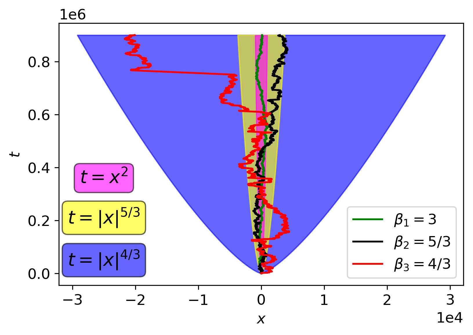
Figure 1: Lévy walk trajectories for three different values of $\beta$, alongside the corresponding asymptotic scaling regimes, for $v=t_{0}=1$. For $\beta>2$ the Lévy walk effectively reduces to Brownian motion, as depicted by the green trajectory for $\beta_{1}=3$ which is contained within the diffusive scaling regime $t=x^{2}$ (magenta). The black trajectory for $\beta_{2}=5/3$, contained within the superdiffusive scaling regime $t=\left|x\right|^{5/3}$ (yellow), consists of “mostly diffusive” motion that is occasionally interrupted by long bouts of ballistic motion. These ballistic bouts become more frequent, pronounced and erratic in the red trajectory for $\beta_{3}=4/3$, confined to the superdiffusive scaling regime $t=\left|x\right|^{4/3}$.

The Model - The 1d Lévy walk of order $\beta$ describes “walkers” moving on the infinite line. Their motion consists of many random excursions, all with a fixed velocity magnitude $v$ but each along a random direction and lasting a random duration $u$ drawn from the distribution

$$\phi\left(u\right)=\beta t_{0}^{\beta}\theta\left[u-t_{0}\right]u^{-1-\beta}.$$ (1)

The step function $\theta\left[x\right]$ keeps $\phi\left(u\right)$ normalizable by imposing a cutoff at the minimal walk time $t_{0}>0$.

Figure 1 demonstrates a single Lévy walk trajectory for different values of $\beta$, qualitatively illustrating the difference between simple Brownian motion and the superdiffusive Lévy walk. For $\beta>2$, both the first and second moments of $\phi\left(u\right)$ are finite and the Lévy walk effectively reduces to Brownian motion (zumofen1993scale, ; zaburdaev2015levy, ). For $1<\beta<2$, which corresponds to the superdiffusive regime considered in this letter, the average walk time remains finite but the second moment diverges, occasionally giving rise to very long excursions which grow increasingly more probable as $\beta\rightarrow 1$. We hereafter restrict our discussion to the superdiffusive regime of $1<\beta<2$.

The probability of finding the walker inside the interval $\left(x,x+\mathbf{d}x\right)$ at time $t$ for an initial condition $P\left(x,0\right)=\delta\left(x\right)$ satisfies the integral equation (dhar2013exact, ; zaburdaev2015levy, )

$$P\left(x,t\right)=0.5\psi\left(t\right)\delta\left(\left|x\right|-vt\right)$$

$$+0.5\int_{0}^{t}\mathbf{d}u\phi\left(u\right)\left[P\left(x-vu,t-u\right)+P\left(x+vu,t-u\right)\right],$$ (2)

where $\psi\left(u\right)$ is the probability of drawing a walk-time greater than $u$, i.e.

$$\psi\left(u\right)=\int_{u}^{\infty}\mathbf{d}w\phi\left(w\right)=1-\theta\left[u-t_{0}\right]\left(1-\left(t_{0}/u\right)^{\beta}\right).$$ (3)

The first line of Eq. (2) describes the walker’s probability to reach $x$ at time $t$ during its initial excursion while the second describes its probability of arriving to $x$ at time $t$ following a previous excursion which ended at position $x\pm vu$ at time $t-u$.

After a Fourier-Laplace transform (see Sec. I of the SM), Eq. (2) for $P\left(x,t\right)$ becomes

$$\tilde{P}\left(k,s\right)=\frac{\tilde{\psi}\left(s-ivk\right)+\tilde{\psi}\left(s+ivk\right)}{2-\tilde{\phi}\left(s-ivk\right)-\tilde{\phi}\left(s+ivk\right)}.$$ (4)

Here $\tilde{P}\left(k,s\right)=\int_{0}^{\infty}\mathbf{d}te^{-st}\hat{P}\left(k,t\right)$ is the Laplace transform of the Fourier transformed probability distribution $\hat{P}\left(k,t\right)=\int_{-\infty}^{\infty}\mathbf{d}xe^{-ikx}P\left(x,t\right)$, $\tilde{\phi}\left(s\pm ivk\right)$ and $\tilde{\psi}\left(s\pm ivk\right)$ are the respective Fourier-Laplace transforms of $\phi\left(t\right)$ and $\psi\left(t\right)$, and $\left\{k,s\right\}$ are the respective Fourier/Laplace conjugates of $\left\{x,t\right\}$.

Main Results - The forthcoming analysis and results are presented in Fourier space, since only there does the probability distribution admit a closed form. The leading correction to the asymptotic distribution $\hat{P}_{0}\left(t\left|k\right|^{\beta}\right)$ is found to be

$$\frac{\hat{P}\left(k,t\right)}{\hat{P}_{0}\left(t\left|k\right|^{\beta}\right)}\approx\begin{cases}\exp\left[-D_{1}t\left|k\right|^{2\beta-1}\right]&\beta<\beta_{c}\\ \exp\left[-D_{2}tk^{2}\right]&\beta>\beta_{c}\end{cases},$$ (5)

where

$$\hat{P}_{0}\left(t\left|k\right|^{\beta}\right)=e^{-D_{0}t\left|k\right|^{\beta}},$$ (6)

and the diffusion coefficients $D_{0},D_{1}$ and $D_{2}$ are provided explicitly in Eq. (16). This correction, which describes the approach of $\hat{P}\left(k,t\right)$ towards its asymptotic scaling form $\hat{P}_{0}\left(t\left|k\right|^{\beta}\right)$, remarkably undergoes a transition as $\beta$ crosses the critical value $\beta_{c}=3/2$: For $\beta>\beta_{c}$, the leading correction scales diffusively as $\left|k\right|\propto t^{-1/2}$ while for $\beta<\beta_{c}$ it remains superdiffusive, scaling as $\left|k\right|\propto t^{-1/\left(2\beta-1\right)}$. The transition is shown to depend only on the tail behavior of $\phi\left(u\right)$ and is thus argued to be universal. The leading correction to the asymptotic truncated MSD similarly undergoes a transition at $\beta=\beta_{c}$. For large $t$, the truncated MSD $\left\langle X\left(t\right)^{2}\right\rangle=\int_{-c\left(vt\right)^{1/\beta}}^{c\left(vt\right)^{1/\beta}}\mathbf{d}xx^{2}P\left(x,t\right)$ takes the form $\left\langle X\left(t\right)^{2}\right\rangle\approx\left\langle X\left(t\right)^{2}\right\rangle_{0}+\delta\left\langle X\left(t\right)^{2}\right\rangle$, where $c\sim\mathcal{O}\left(1\right)$ is an arbitrary constant,

$$\left\langle X\left(t\right)^{2}\right\rangle_{0}=h_{0}v\left(vt\right)^{2/\beta},$$ (7)

and

$$\delta\left\langle X\left(t\right)^{2}\right\rangle=-\begin{cases}D_{1}h_{2\beta-1}\left(vt\right)^{\frac{3-\beta}{\beta}}&\beta<\beta_{c}\\ D_{2}h_{2}vt&\beta>\beta_{c}\end{cases},$$ (8)

with $h_{\gamma}$ provided in Eq. (18).

The analytical results for $\hat{P}\left(k,t\right)$ in Eq. (5) are supplemented by numerical simulation results of the Lévy walk’s dynamics, denoted by $\hat{P}_{sim}\left(k,t\right)$, and by the numerical inverse-Laplace transform of the exact Eq. (4) for the distribution, denoted by $\hat{P}_{num}\left(k,t\right)$. Figure 2 plots the temporal evolution of $\log\left[\hat{P}\left(k,t\right)\right]$ versus $k$ while Fig. 3 plots $\log\left[\hat{P}\left(k,t\right)/\hat{P}_{0}\left(t\left|k\right|^{\beta}\right)\right]$ versus $D_{1}t\left|k\right|^{2\beta-1}$ and $D_{2}tk^{2}$ for $\beta=4/3<\beta_{c}$ and $\beta=5/3>\beta_{c}$, respectively. Both figures illustrate an excellent agreement between the correction provided in Eq. (5) and both the simulation and numerical analysis. A figure comparing the results in Eqs. (7) and (8) for the truncated MSD to the results of direct numerical simulations of the Lévy walk model is given in Sec. II of the SM. Additional details regarding the simulation procedure are provided in Sec. VI of the SM.

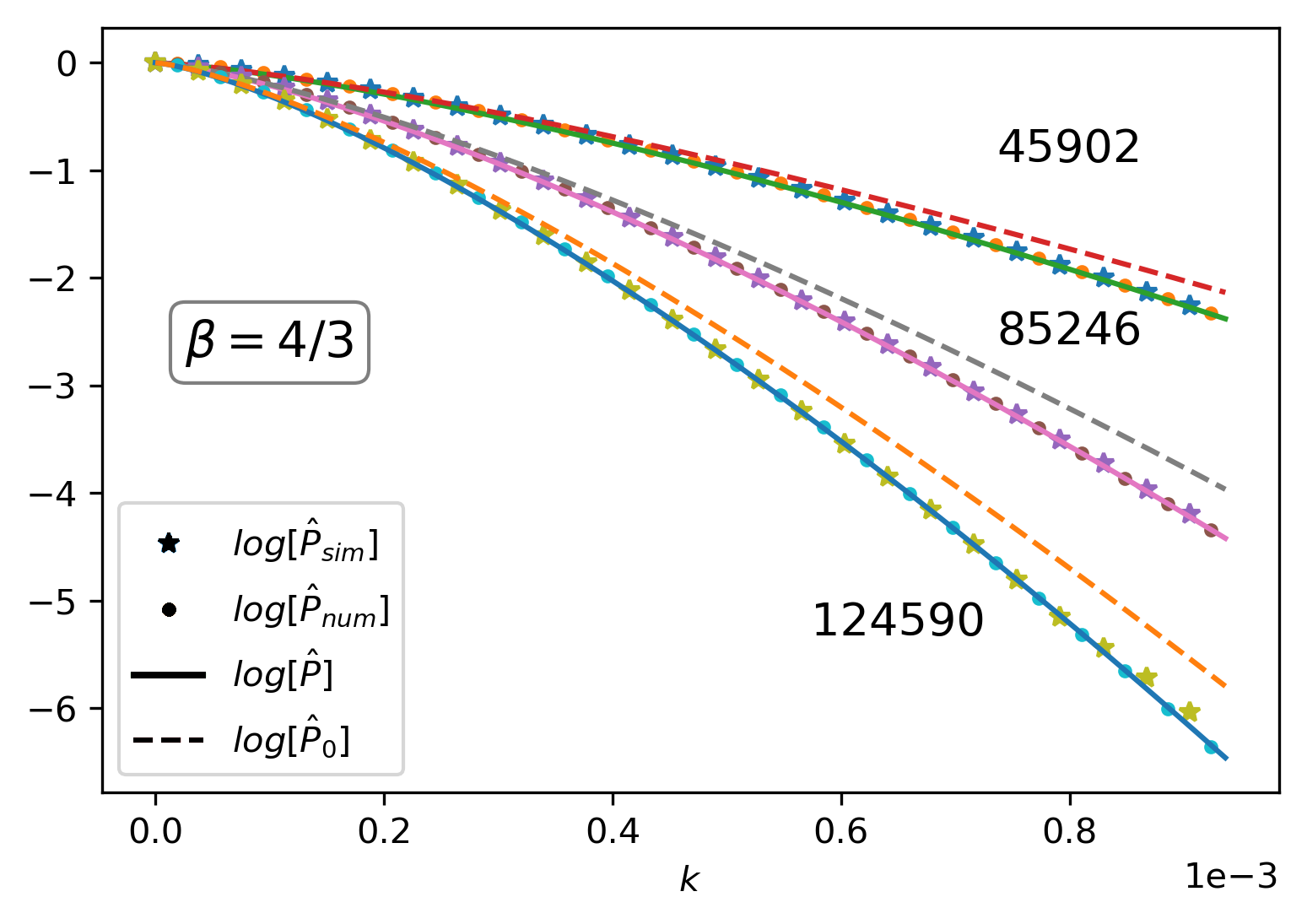
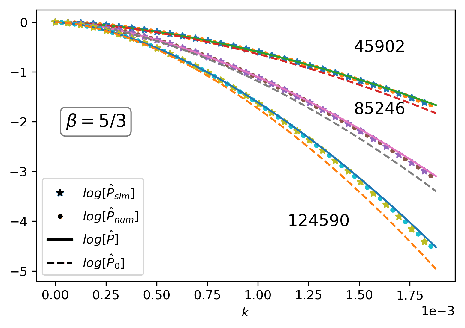
Figure 2: A log-plot of the probability distribution for small $\left|k\right|$, long-times (indicated near each curve) and $v=t_{0}=1$. Stars denote simulation data $\hat{P}_{sim}\left(k,t\right)$, dots denote the numerical solution $\hat{P}_{num}\left(k,t\right)$, solid curves denote $\hat{P}\left(k,t\right)$ and dashed curves denote the asymptotic solution $\hat{P}_{0}\left(t\left|k\right|^{\beta}\right)$.

Asymptotic Analysis - To obtain the leading correction to the asymptotic probability distribution, our strategy will be to study $\tilde{P}\left(k,s\right)$ in the following order of limits: We first retrieve the leading behavior of $\tilde{P}\left(k,s\right)$ for small $s$ (i.e. large $t$), then take the inverse Laplace transform and finally extract the leading correction to $\hat{P}_{0}\left(t\left|k\right|^{\beta}\right)$ in the scaling limit $\left|k\right|\rightarrow 0$, $t\rightarrow\infty$ with $t\left|k\right|^{\beta}$ kept constant. It will prove convenient to transform to the dimensionless variables

$$\sigma=t_{0}s\text{ };\text{ }\tau=t/t_{0}\text{ ; }q=\ell_{0}k,$$ (9)

where $\ell_{0}=t_{0}v$ denotes the typical length-scale of the model. As demonstrated in Sec. III of the SM, only the leading term in the expansion of $\tilde{\psi}\left(\sigma-iq\right)+\tilde{\psi}\left(\sigma+iq\right)$ of Eq. (4) in small $\sigma$ and $\left|q\right|$ enters the leading correction. This agrees with intuition, as $\psi\left(t\right)$ in Eq. (2) for $P\left(x,t\right)$ describes the walker’s probability of arriving to $x$ at time $t$ during its initial excursion. This process naturally becomes irrelevant in the scaling limit, as $\left|x\right|$ and $t$ grow larger.

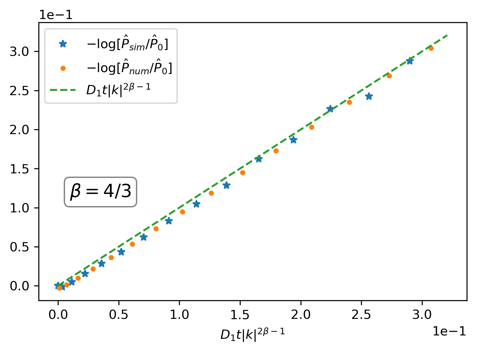
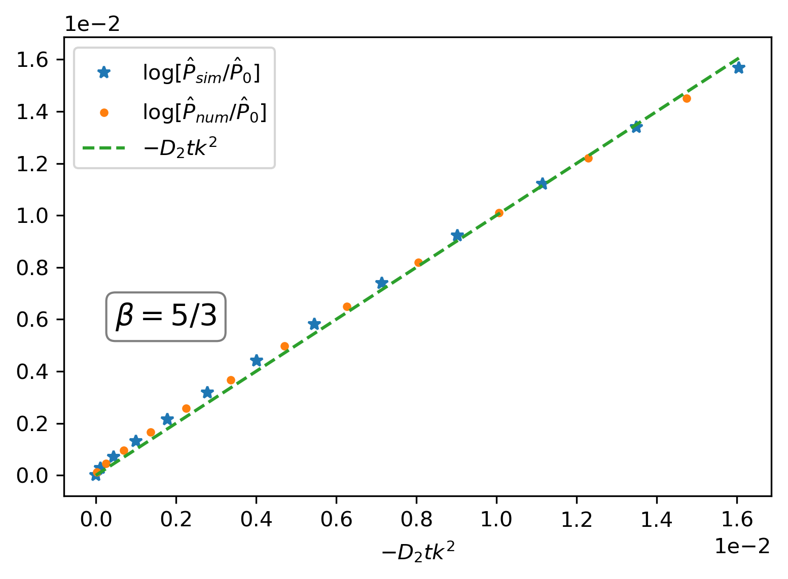
Figure 3: A log-plot of the probability distribution divided by the asymptotic solution versus $D_{1}t\left|k\right|^{2\beta-1}$ and $-D_{2}tk^{2}$ for $\beta=4/3$ and $\beta=5/3$, respectively. The data was obtained for a large time $t\sim\mathcal{O}\left(10^{7}\right)$ and $v=t_{0}=1$. Blue stars denote simulation data $\hat{P}_{sim}\left(k,t\right)$, orange dots denote the numerical solution $\hat{P}_{num}\left(k,t\right)$ and the dashed green line is provided as a guide for the eye.

We next consider the small-$\sigma$ behavior of $\tilde{\phi}\left(\sigma\mp iq\right)$, which appears in the denominator of Eq. (4). Expanding the Laplace transform to first order in $\sigma$ yields

$$\tilde{\phi}\left(\sigma\mp iq\right)\approx\int_{0}^{\infty}\mathbf{d}\tau\phi\left(\tau\right)e^{\pm iq\tau}\left(1-\sigma\tau\right).$$ (10)

With this, the large time behavior of $\tilde{P}\left(q,\sigma\right)$ is recovered as

$$\tilde{P}\left(q,\sigma\right)\approx\frac{\beta}{\beta-1}\frac{1}{A\left(q\right)+B\left(q\right)\sigma},$$ (11)

whose inverse Laplace transform is

$$\hat{P}\left(q,\tau\right)\approx\left(\frac{\beta}{\beta-1}\frac{1}{B\left(q\right)}\right)e^{-I\left(q\right)\tau}.$$ (12)

Here we have defined

$$I\left(q\right)=A\left(q\right)/B\left(q\right),$$ (13)

where the functions $A\left(q\right)$ and $B\left(q\right)$ are given by

$$\begin{array}[]{c}A\left(q\right)=1-\left\langle\cos\left[qu\right]\right\rangle_{u}\approx a\left|q\right|^{\beta}-\frac{\beta q^{2}}{2\left(2-\beta\right)}+\mathcal{O}\left(q^{4}\right)\\ B\left(q\right)=\partial_{q}\left\langle\sin\left[qu\right]\right\rangle_{u}\approx\frac{\beta}{\beta-1}+b\left|q\right|^{\beta-1}+\mathcal{O}\left(q^{2}\right)\end{array},$$ (14)

with $a=\cos\left[\pi\beta/2\right]\Gamma\left[1-\beta\right]$ and $b=\beta\sin\left[\pi\beta/2\right]\Gamma\left[1-\beta\right]$ such that $a>0$ and $b<0$ for $1<\beta<2$. We have also used $\left\langle f\left(q,u\right)\right\rangle_{u}=\int_{0}^{\infty}\mathbf{d}u\phi\left(u\right)f\left(q,u\right)$ to denote the expectation value with respect to $u$ and $\Gamma\left[x\right]$ to denote the Euler gamma function.

The long-time behavior of $\hat{P}\left(q,\tau\right)$ finally emerges: Upon defining the scaling variable $\left|z\right|=\tau\left|q\right|^{\beta}$ and taking the scaling limit, the pre-factor $\left(\frac{\beta}{\beta-1}\frac{1}{B\left(q\right)}\right)$ in Eq. (12) reduces to unity and $I\left(q\right)\tau$ becomes

$$c_{0}\left|z\right|-c_{1}\left|z\right|^{\frac{2\beta-1}{\beta}}\tau^{-\frac{\beta-1}{\beta}}-c_{2}\left|z\right|^{\frac{2}{\beta}}\tau^{-\frac{2-\beta}{\beta}},$$ (15)

where $c_{0}=a\left(\beta-1\right)/\beta$, $c_{1}=c_{0}^{2}b/a$, $c_{2}=\left(\beta-1\right)/\left(4-2\beta\right)$ and faster decaying terms of $\sim\mathcal{O}\left(\tau^{-\left(\beta+1\right)/\beta}\right)$ are neglected. Reinstating $\left\{q,\tau\right\}$ in place of $z$ and replacing the dimensionless variables $\left\{q,\tau\right\}$ by $\left\{k,t\right\}$ via Eq. (9) yields $\hat{P}\left(k,t\right)$ of Eq. (5) with the diffusion coefficients given by

$$D_{0}=c_{0}\ell_{0}^{\beta}/t_{0}\text{ };\text{ }D_{1}=-c_{1}\ell_{0}^{2\beta-1}/t_{0}\text{ };\text{ }D_{2}=-c_{2}\ell_{0}^{2}/t_{0}.$$ (16)

A typical quantity of interest in studies of superdiffusive systems is the MSD. Having derived the leading correction to $\hat{P}_{0}\left(\left|k\right|^{\beta}t\right)$, we next analyze the leading correction to the asymptotic truncated MSD $\left\langle X\left(t\right)^{2}\right\rangle_{0}$ for a walker that is initially located at the origin. Since $P\left(x,t\right)$ describes a superdiffusive process, the MSD $\int_{-\infty}^{\infty}\mathbf{d}xx^{2}P\left(x,t\right)$ diverges when integrated over the infinite line. Limiting the domain to $x\in\left[-c\left(vt\right)^{1/\beta},c\left(vt\right)^{1/\beta}\right]$, where $c$ is an arbitrary $c\sim\mathcal{O}\left(1\right)$ constant, provides the temporal scaling of this divergence giving

$$\left\langle X\left(t\right)^{2}\right\rangle=\left(vt\right)^{2/\beta}\int_{-\infty}^{\infty}\mathbf{d}\kappa\hat{P}\left(\kappa\left(vt\right)^{-1/\beta},t\right)g\left(\kappa\right),$$ (17)

where $P\left(x,t\right)$ was replaced by its Fourier transform, $g\left(\kappa\right)=\left(2c\kappa\cos\left[c\kappa\right]-\left(2-c^{2}\kappa^{2}\right)\sin\left[c\kappa\right]\right)/\left(\pi\kappa^{3}\right)$ and the change of variables $\kappa=k\left(vt\right)^{1/\beta}$ was used. Substituting $\hat{P}\left(k,t\right)$ of Eq. (5) and expanding in large $t$ up to the leading correction yields Eqs. (7) and (8), with the coefficient $h_{\gamma}$ given by

$$h_{\gamma}=v^{-1}\int_{-\infty}^{\infty}\mathbf{d}\kappa e^{-v^{-1}D_{0}\left|\kappa\right|^{\beta}}g\left(\kappa\right)\left|\kappa\right|^{\gamma}.$$ (18)

Universality of $\beta_{c}$ - We next argue that the transition at $\beta_{c}=3/2$ is universal by deriving it from a general walk-time distribution whose tail has the form $\sim u^{-1-\beta}$. To this end, recall that in Eq. (12) we found that the large-time properties of $\hat{P}\left(k,t\right)$ are determined by $I\left(q\right)$. As such, we turn our attention to it. Since the duration of a walk cannot be negative, $\phi\left(u\right)$ must vanish for $u<0$. Thus, the integration range in $\left\langle\cos\left[qu\right]\right\rangle_{u}$ and $\left\langle\sin\left[qu\right]\right\rangle_{u}$ of Eq. (14) can be safely extended to $u\in\left(-\infty,+\infty\right)$, allowing $I\left(q\right)$ to be rewritten as

$$I\left(q\right)=\left(1-\text{Re}\left[\hat{\phi}\left(q\right)\right]\right)/\partial_{q}\text{Im}\left[\hat{\phi}\left(q\right)\right],$$ (19)

where $\hat{\phi}\left(\pm q\right)=\int_{-\infty}^{\infty}\mathbf{d}u\phi\left(u\right)e^{\mp iqu}$ is the characteristic function of $\phi\left(u\right)$, whose Hermitian property $\hat{\phi}\left(-q\right)=\hat{\phi}\left(q\right)^{*}$ was used to obtain Eq. (19).

The ground is now set to hold a more general discussion on the structure of $I\left(q\right)$: Since $\phi\left(u\right)$ is one-sided, it is non-symmetric and so its Fourier transform $\hat{\phi}\left(q\right)$ contains both real and imaginary terms. Now, had all of the moments of $\phi\left(u\right)$ been finite, $\hat{\phi}\left(q\right)$ would have been an analytic function whose $n^{th}$ power-series coefficient in $q$ would simply be $\propto\left(i\right)^{n}\left\langle u^{n}\right\rangle_{u}$. However, due to its heavy tail, the moments of $\phi\left(u\right)$ are not all finite and so additional non-analytic terms must also show up in $\hat{\phi}\left(q\right)$. It is straightforward to show that a heavy tail $\sim u^{-1-\beta}$ in $\phi\left(u\right)$ does indeed result in real and imaginary non-analytic terms in $\hat{\phi}\left(q\right)$ which are $\propto\left|q\right|^{\beta}$. Therefor, $\hat{\phi}\left(q\right)$ must be the sum of two parts: The first being an analytic power-series in $q$ while the second contains non-analytic terms $\propto\left|q\right|^{\beta}$. We thus write $\hat{\phi}\left(q\right)$ as $\hat{\phi}\left(q\right)=\text{Re}\left[\hat{\phi}\left(q\right)\right]+i\text{Im}\left[\hat{\phi}\left(q\right)\right]$ with

$$\begin{cases}\text{Re}\left[\hat{\phi}\left(q\right)\right]=\sum_{n=0}^{\infty}\omega_{2n}q^{2n}+d_{1}\left|q\right|^{\beta}\\ \text{Im}\left[\hat{\phi}\left(q\right)\right]=\sum_{n=0}^{\infty}\omega_{2n+1}q^{2n+1}+d_{2}\left|q\right|^{\beta}\end{cases},$$ (20)

where $\omega_{n}$ are $q$-independent coefficients while $d_{1}$ and $d_{2}$ may depend on the sign of $q$. Since $\phi\left(u\right)$ is normalized $\hat{\phi}\left(q=0\right)$ is equal to unity, setting $\omega_{0}=1$. With this, the small-$\left|q\right|$ approximation of $I\left(q\right)$ becomes

$$I\left(q\right)\approx\left(d_{1}\left|q\right|^{\beta}+\omega_{2}q^{2}\right)/\left(\omega_{1}+\beta d_{2}\left|q\right|^{\beta-1}\right).$$ (21)

Equation (21) has the same structure as in Eqs. (14) and (15) and must therefor also lead to a transition at $\beta_{c}=3/2$. We call this transition universal since, as we have just shown, it can be derived under fairly general considerations, namely that the tail of $\phi\left(u\right)$ has the form $\sim u^{-1-\beta}$. The characteristic function $\hat{\phi}\left(q\right)$ is explicitly computed in Sec. IV of the SM, showing it is indeed of the same form as in Eq. (20). $I\left(q\right)$ is computed for a different walk-time distribution, which shares only its heavy tail $\sim u^{-1-\beta}$ with $\phi\left(u\right)$, and the same transition is recovered at $\beta_{c}=3/2$ in section V of the SM.

Conclusions - In this letter, the approach of the probability distribution of a superdiffusive system towards its asymptotic form was studied using the Lévy walk of order $1<\beta<2$. This approach, described by the leading correction to the asymptotic distribution, was shown to undergo a transition at the critical value $\beta_{c}=3/2$, at which its scaling remarkably changes from diffusive to superdiffusive. The leading correction to the asymptotic MSD also undergoes a transition at the same $\beta_{c}$. The transition was argued to be universal as it depends only on the tail behavior of the walk time distribution.

These results are especially useful since they can readily be applied to study the many superdiffusive systems modeled by Levy walks, whose finite-time corrections are often unavoidable and devastating. Such corrections are known to pose a significant challenge in the study of anomalous heat transport (denisov2003dynamical, ; cipriani2005anomalous, ; dhar2013exact, ; lepri2016thermal, ; cividini2017temperature, ; miron2019derivation, ; PhysRevE.100.012106, ). For example, the Lévy walk of order $\beta=5/3$ was used in (cipriani2005anomalous, ) to model the leading asymptotic superdiffusive spreading of energy perturbations and entailing anomalous transport of a 1d Hamiltonian system. Yet the connection between anomalous transport and Lévy walks is suggested to extend to an entire class of similar models (cipriani2005anomalous, ). Indeed, a diffusive correction to the asymptotic anomalous energy spreading and heat current have recently been reported in a stochastic 1d gas system (miron2019derivation, ). A diffusive correction to the current was similarly derived under nonequilibrium settings for the 1d Lévy walk of order $\beta>3/2$ in (PhysRevE.100.012106, ). Both of these results are consistent with the findings reported in this letter. It would thus be of great interest to further test these results in additional experimental and numerical superdiffusive setups, especially ones modeled by Lévy walks with $\beta<\beta_{c}$. It would also be very interesting to study the onset of superdiffusion in the related Lévy flight model where particles draw a “flight distance”, rather than a walk time, immediately materializing at their new location (shlesinger1986levy, ; dubkov2008levy, ; zaburdaev2015levy, ).

Acknowledgments - I thank David Mukamel for his ongoing encouragement and support and for many helpful discussions. I also thank Hillel Aharony, Julien Cividini, Anupam Kundu, Bertrand Lacroix-A-Chez-Toine and Oren Raz for critically reading this manuscript and for their helpful remarks. This work was supported by a research grant from the Center of Scientific Excellence at the Weizmann Institute of Science.

Supplemental Material

I Fourier-Laplace Transform of Eq. $\left(2\right)$

This section outlines the derivation of the Fourier-Laplace transformed probability distribution $\tilde{P}\left(k,s\right)$ in Eq. $\left(4\right)$ of the main text. We start from the main text Eq. $\left(2\right)$ for the walker’s position probability distribution, $P\left(x,t\right)$. Taking first a Fourier transform of the equation, using $\hat{P}\left(k,t\right)=\int_{-\infty}^{\infty}\mathbf{d}xe^{ikx}P\left(x,t\right)$, we obtain

$$\hat{P}\left(k,t\right)=\psi\left(t\right)\cos\left(ktv\right)$$

$$+\frac{1}{2}\int_{0}^{t}\mathbf{d}u\phi\left(u\right)\biggl{[}\int_{-\infty}^{\infty}\mathbf{d}ze^{ik\left(z+vu\right)}P\left(z,t-u\right)$$

$$+\int_{-\infty}^{\infty}\mathbf{d}ze^{ik\left(z-vu\right)}P\left(z,t-u\right)\biggl{]}$$

$$=\psi\left(t\right)\cos\left(ktv\right)$$

$$+\int_{0}^{t}\mathbf{d}u\phi\left(u\right)\hat{P}\left(k,t-u\right)\cos\left(kvu\right).$$ (22)

Next taking a Laplace transform, i.e. $\tilde{P}\left(k,s\right)=\int_{0}^{\infty}\mathbf{d}te^{-st}\hat{P}\left(k,t\right)$, of Eq. (22) yields

$$\tilde{P}\left(k,s\right)=\frac{1}{2}\biggl{(}\int_{0}^{\infty}\mathbf{d}te^{-t\left(s-ikv\right)}\psi\left(t\right)$$

$$+\int_{0}^{\infty}\mathbf{d}te^{-t\left(s+ikv\right)}\psi\left(t\right)\biggl{)}+\frac{1}{2}\int_{0}^{\infty}\mathbf{d}te^{-st}$$

$$\times\int_{0}^{t}\mathbf{d}u\phi\left(u\right)\hat{P}\left(k,t-u\right)\left(e^{ikuv}+e^{-ikuv}\right)$$

$$=\frac{1}{2}\left[\tilde{\psi}\left(s-ikv\right)+\tilde{\psi}\left(s+ikv\right)\right]$$

$$+\frac{1}{2}\tilde{P}\left(k,s\right)\left[\tilde{\phi}\left(s-ikv\right)+\tilde{\phi}\left(s+ikv\right)\right].$$ (23)

Isolating $\tilde{P}\left(k,s\right)$ then gives the main text Eq. $\left(4\right)$, $\tilde{P}\left(k,s\right)=\frac{\tilde{\psi}\left(s-ikv\right)+\tilde{\psi}\left(s+ikv\right)}{2-\tilde{\phi}\left(s-ivk\right)-\tilde{\phi}\left(s+ivk\right)}$.

II The Truncated MSD

In this section the theoretical expressions for the truncated mean-square displacement (MSD) are compared to the results of direct numerical simulations of the Lévy walk model for $\beta=4/3$ and for $\beta=5/3$. As shown in the main text Eqs. $\left(7\right)$ and $\left(8\right)$, at large times the MSD is given by

$$\left\langle X\left(t\right)^{2}\right\rangle=\int_{-c\left(vt\right)^{1/\beta}}^{c\left(vt\right)^{1/\beta}}\mathbf{d}xx^{2}P\left(x,t\right)$$

$$\approx\left\langle X\left(t\right)^{2}\right\rangle_{0}+\delta\left\langle X\left(t\right)^{2}\right\rangle,$$ (24)

where $c$ is an arbitrary $\sim\mathcal{O}\left(1\right)$ constant and $P\left(x,t\right)$ is obtained via an inverse Fourier transform of $\hat{P}\left(k,t\right)$ in the main text Eq. $\left(5\right)$. The asymptotic MSD is given by

$$\left\langle X\left(t\right)^{2}\right\rangle_{0}=h_{0}v\left(vt\right)^{2/\beta},$$ (25)

the leading correction is given by

$$\delta\left\langle X\left(t\right)^{2}\right\rangle=-\begin{cases}D_{1}h_{2\beta-1}\left(vt\right)^{\frac{3-\beta}{\beta}}&\beta<\beta_{c}\\ D_{2}h_{2}vt&\beta>\beta_{c}\end{cases},$$ (26)

and $h_{\gamma}$ is given in the main text Eq. $\left(18\right)$. The simulated MSD is denoted by $\left\langle X\left(t\right)^{2}\right\rangle_{sim}$ and computed from Eq. (24) by replacing $P\left(x,t\right)$ by $P_{sim}\left(x,t\right)$ (i.e. the simulated probability distribution). Details on the calculation of $P_{sim}\left(x,t\right)$ are provided in Sec. VI.

Figure 4 plots $\left\langle X\left(t\right)^{2}\right\rangle$ and $\left\langle X\left(t\right)^{2}\right\rangle_{sim}$ versus time and the insets show $\left\langle X\left(t\right)^{2}\right\rangle/t^{2/\beta}$ and $\left\langle X\left(t\right)^{2}\right\rangle_{sim}/t^{2/\beta}$ versus $t$. Notice that the calculation of $\left\langle X\left(t\right)^{2}\right\rangle$ relays on the large-$t$ and large-$\left|x\right|$ approximation of the distribution, $P\left(x,t\right)$. However, since the simulated $\left\langle X\left(t\right)^{2}\right\rangle_{sim}$ is computed over the range $x\in\left[-c\left(vt\right)^{1/\beta},c\left(vt\right)^{1/\beta}\right]$ which includes regions in which $\left|x\right|$ is small. As such, a constant offset of $\sim\mathcal{O}\left(1\right)\%$ is visible between simulation and theory in Fig. 4. Nevertheless, the temporal scaling of the MSD is unaffected by this offset and a very good agreement is found between simulation and theory.

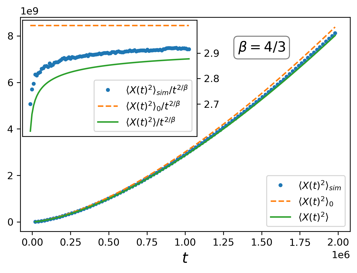
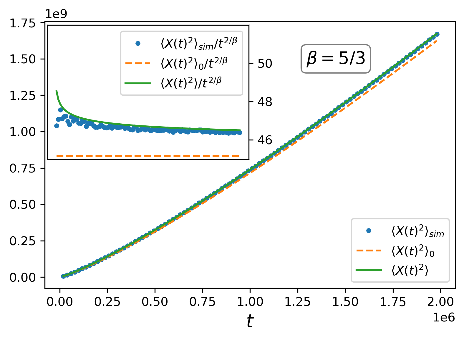
Figure 4: The simulated and theoretical MSD plotted versus $t$ for $\beta=4/3$ and $\beta=5/3$. The inset shows the MSD scaled by $t^{2/\beta}$ versus $t$ for both values of $\beta$. Blue stars denote simulation data, dashed orange curves denote the asymptotic solution and green solid curves denote the corrected solution. For $\beta=4/3$ the constant $c$ was set to $1$ while for $\beta=5/3$ we take $c=5$. The parameters $v=t_{0}=10$ were chosen to clearly separate the asymptotic solution from its leading correction for both values of $\beta$.

III Expansion of $\tilde{\psi}\left(\sigma-iq\right)+\tilde{\psi}\left(\sigma+iq\right)$

In this section we show that only the leading term in the expansion of $\tilde{\psi}\left(\sigma-iq\right)+\tilde{\psi}\left(\sigma+iq\right)$ for small $\sigma$ and $\left|q\right|$ (i.e. large times and distances), which appears in the numerator of the main text Eq. $\left(4\right)$, contributes to the leading correction to the distribution. As in the calculation of $\tilde{\phi}\left(\sigma\pm iq\right)$ of the main text Eq. $\left(10\right)$, we shall first expand in small $\sigma$ (i.e. large $t$), neglecting corrections of $\mathcal{O}\left(\sigma^{2}\right)$,

$$\tilde{\psi}\left(\sigma-iq\right)+\tilde{\psi}\left(\sigma+iq\right)$$

$$\approx 2\biggl{[}\int_{0}^{\infty}\mathbf{d}\tau\psi\left(\tau\right)\cos\left[q\tau\right]$$

$$-\partial_{q}\left(\int_{0}^{\infty}\mathbf{d}\tau\psi\left(\tau\right)\sin\left[q\tau\right]\right)\sigma\biggl{]}.$$ (27)

Next, expanding in small $\left|q\right|$ this becomes

$$\tilde{\psi}\left(\sigma-iq\right)+\tilde{\psi}\left(\sigma+iq\right)\approx m+n\left|q\right|^{\beta-1}$$

$$+pq^{2}-\left(r-w\left|q\right|^{\beta-2}+zq^{2}\right)\sigma+\mathcal{O}\left(q^{3}\right),$$ (28)

with the following coefficients

$$\begin{cases}m=\frac{2\beta}{\beta-1}\text{ };&n=2\sin\left[\frac{\pi\beta}{2}\right]\Gamma\left[1-\beta\right]\\ p=\frac{\beta}{3\left(3-\beta\right)}\text{ };&r=\frac{\beta}{\beta-2}\\ w=2\cos\left[\frac{\pi\beta}{2}\right]\Gamma\left[2-\beta\right]\text{ };&z=\frac{\beta}{4\left(4-\beta\right)}\end{cases}.$$ (29)

Repeating this scheme for $2-\tilde{\phi}\left(\sigma-iq\right)-\tilde{\phi}\left(\sigma+iq\right)$, which appears in the denominator of the main text Eq. $\left(4\right)$, yields

$$2-\tilde{\phi}\left(\sigma-iq\right)-\tilde{\phi}\left(\sigma+iq\right)$$

$$\approx G\left|q\right|^{\beta}+Hq^{2}+\sigma\left(J+M\left|q\right|^{\beta-1}+Pq^{2}\right)+\mathcal{O}\left(q^{3}\right),$$ (30)

with the coefficients

$$\begin{cases}G=2\cos\left[\frac{\pi\beta}{2}\right]\Gamma\left[1-\beta\right]\text{ };&H=\frac{\beta}{\beta-2}\\ J=\frac{2\beta}{\beta-1}\text{ };&M=2\beta\sin\left[\frac{\pi\beta}{2}\right]\Gamma\left[1-\beta\right]\\ P=\frac{\beta}{3-\beta}\end{cases}.$$ (31)

Finally, substituting both $\tilde{\psi}\left(\sigma-iq\right)+\tilde{\psi}\left(\sigma+iq\right)$ of Eq. (28) and $2-\tilde{\phi}\left(\sigma-iq\right)-\tilde{\phi}\left(\sigma+iq\right)$ of Eq. (30) into the main text Eq. $\left(4\right)$ gives

$$\tilde{P}\left(q,\sigma\right)\approx\frac{m+n\left|q\right|^{\beta-1}+pq^{2}-\left(r-w\left|q\right|^{\beta-2}+zq^{2}\right)\sigma}{G\left|q\right|^{\beta}+Hq^{2}+\sigma\left(J+M\left|q\right|^{\beta-1}+Pq^{2}\right)}.$$ (32)

Replacing the numerator $\tilde{\psi}\left(\sigma-iq\right)+\tilde{\psi}\left(\sigma+iq\right)$ by its leading correction $m$, as done in deriving the main text Eq. $\left(11\right)$, is justified at $\sim\mathcal{O}\left(\sigma\right)$ and for small $\left|q\right|$ if the leading terms in the expansion of $\tilde{P}\left(q,\sigma\right)$ is independent of all of the other coefficients in Eq. (29) (i.e. the coefficients denoted by lower-case letters). A straightforward calculation verifies that this is true.

IV The Structure of $\hat{\phi}\left(q\right)$

In this section we compute the characteristic function $\hat{\phi}\left(q\right)$ of the walk time distribution $\phi\left(u\right)=\beta t_{0}^{\beta}\frac{\theta\left[u-t_{0}\right]}{u^{1+\beta}}$ of the main text Eq. $\left(1\right)$ and show it has the same form recovered in the main text Eq. $\left(20\right)$ for a general distribution with the same tail behavior. By definition, the characteristic function $\hat{\phi}\left(q\right)$ is given by $\hat{\phi}\left(q\right)=\int_{-\infty}^{\infty}\mathbf{d}u\phi\left(u\right)e^{-iqu}$. Carrying out the integration yields

$$\hat{\phi}\left(q\right)=f\left(q;\beta\right)-i\frac{\beta}{\beta-1}qg\left(q;\beta\right)$$

$$+\beta\Gamma\left[-\beta\right]\left(\cos\left[\frac{\pi\beta}{2}\right]+i\sin\left[\frac{\pi\beta}{2}\right]\text{sgn}\left[q\right]\right)\left|q\right|^{\beta}.$$ (33)

The first line of Eq. (33) contains generalized hypergeometric functions, which we denote by $f\left(q;\beta\right)$ and $g\left(q;\beta\right)$, that are given by

$$\begin{cases}f\left(q;\beta\right)\coloneqq\mbox{ }_{1}F_{2}\left[\left\{-\frac{\beta}{2}\right\};\left\{\frac{1}{2},\frac{2-\beta}{2}\right\};-\frac{q^{2}}{4}\right]\\ g\left(q;\beta\right)\coloneqq\mbox{ }_{1}F_{2}\left[\left\{\frac{1-\beta}{2}\right\};\left\{\frac{3}{2},\frac{3-\beta}{2}\right\};-\frac{q^{2}}{4}\right]\end{cases}.$$ (34)

The hypergeometric function $\mbox{ }_{p}F_{q}\left[\left\{a_{i}\right\}_{i=1}^{p};\left\{b_{j}\right\}_{j=1}^{q};z\right]$ is a compact notation for the power series

$$\mbox{ }_{p}F_{q}\left[\left\{a_{i}\right\}_{i=1}^{p};\left\{b_{j}\right\}_{j=1}^{q};z\right]=\sum_{n=0}^{\infty}\frac{\left(a_{1}\right)_{n}...\left(a_{p}\right)_{n}}{\left(b_{1}\right)_{n}...\left(b_{q}\right)_{n}}\frac{z^{n}}{n!},$$ (35)

where $\left(y\right)_{n}$ is the Pochhammer symbol, given by

$$\left(y\right)_{n}=\frac{\Gamma\left[y+n\right]}{\Gamma\left[y\right]},$$ (36)

and $\Gamma\left[x\right]$ is the Gamma function. Thus, as argued in the main text, the first part of $\hat{\phi}\left(q\right)$ is analytic in $q$ while the second contains non-analytic terms $\propto\left|q\right|^{\beta}$, that arise due to the heavy tail of $\phi\left(u\right)$.

V A Different Walk Time Distribution

In this section we compute $I\left(q\right)$ in the main text Eq. $\left(19\right)$ for a different choice of walk-time distribution

$$\rho\left(u\right)=\begin{cases}\frac{u_{0}^{\beta}}{\Gamma\left[\beta\right]}\frac{e^{-\frac{u_{0}}{u}}}{u^{1+\beta}}&u\geq 0\\ 0&u<0\end{cases},$$ (37)

that has the same heavy tail as $\phi\left(u\right)$ but a very different short time behavior, showing that the same transition at $\beta_{c}=3/2$ is recovered. One can verify that all of the steps leading to the Fourier transformed probability distribution in the main text for long times and large distances, i.e.

$$\hat{P}\left(q,\tau\right)\approx e^{-I\left(q\right)\tau},$$ (38)

remain valid for $\rho\left(u\right)$ too. We next compute the leading correction to $\hat{P}_{0}\left(\tau\left|q\right|^{\beta}\right)$ from $I\left(q\right)$ of the main text Eq. $\left(19\right)$, using $\hat{\rho}\left(q\right)=\int_{0}^{\infty}\mathbf{d}u\rho\left(u\right)e^{iqu}$, as

$$I\left(q\right)=\frac{1-\text{Re}\left[\hat{\rho}\left(q\right)\right]}{\partial_{q}\text{Im}\left[\hat{\rho}\left(q\right)\right]}.$$ (39)

Expanding $\hat{\rho}\left(q\right)$ in small $\left|q\right|$ yields

$$\hat{\rho}\left(q\right)\approx 1-i\frac{u_{0}}{\beta-1}q-\frac{u_{0}^{2}q^{2}}{2\left(2-3\beta+\beta^{2}\right)}$$

$$-\frac{u_{0}^{\beta}\pi e^{\frac{i\pi\beta}{2}}}{\sin\left[\pi\beta\right]\Gamma\left[\beta\right]\Gamma\left[1+\beta\right]}\left|q\right|^{\beta}.$$ (40)

Substituting this expansion into Eq. (39) for $I\left(q\right)$ then gives

$$I\left(q\right)\approx-\frac{\pi u_{0}^{\beta-1}}{2\sin\left[\pi\beta\right]\Gamma\left[\beta-1\right]\Gamma\left[\beta+1\right]}\biggl{(}2\cos\left[\frac{\pi\beta}{2}\right]\left|q\right|^{\beta}$$

$$-\frac{\beta\pi u_{0}^{\beta-1}\left|q\right|^{2\beta-1}}{\Gamma\left[\beta-1\right]\Gamma\left[\beta+1\right]}\biggl{)}+\frac{Bq^{2}}{2\left(2-\beta\right)},$$ (41)

where higher order corrections in $\left|q\right|$ have been neglected. It is evident that the leading correction to the asymptotic term $\sim\left|q\right|^{\beta}$ changes at the transition $\beta_{c}=3/2$, as found for $\phi\left(u\right)$.

VI Simulation Procedure

In this section we outline the numerical simulation procedure used to obtain the simulated walker probability distribution in Fourier space $\hat{P}_{sim}\left(k,t\right)$ and MSD $\left\langle X\left(t\right)^{2}\right\rangle_{sim}$ which appear in the main text figures. In each realization the walker was initialized at the origin of the interval $\left[-\frac{L}{2},+\frac{L}{2}\right]$ with a velocity of magnitude $v$ pointing towards a random direction $\pm 1$ and a walk time $u$ drawn from the walk time distribution $\phi\left(u\right)$ of the main text Eq. $\left(1\right)$ with cutoff time $t_{0}$. The Lévy walk dynamics were then run up to time $T=0.45\left(L/v\right)$, chosen this way to ensure to ensure that the walker does not escape the interval. The interval was divided into bins of size $\Delta x$ such that $L/\Delta x$ was an integer number. At each time interval $\Delta t$ the walker’s position $X\left(t\right)$ was mapped into the appropriate bin, whose centers are at $x_{m}=\left(m-\frac{1}{2}\right)\Delta x-\frac{L}{2}$, where $m=1,2,...,L/\Delta x$. By repeating this procedure for $\sim\mathcal{O}\left(10^{6}\right)$ realizations, a histogram for the probability $P\left(x_{m},t_{n}\right)$ of finding the walker inside bin $x_{m}$ at time $t_{n}=n\Delta t$ was obtained, where $n=1,2,...,N$ with $N=\frac{T}{\Delta t}$. The simulated Fourier transformed distribution $\hat{P}_{sim}\left(k_{m},t_{n}\right)$ was then obtained by taking a Fourier transform of $P\left(x_{m},t_{n}\right)$, with $k_{m}$ given by $k_{m}=\frac{2\pi m}{L}$. The probability $P\left(x_{m},t_{n}\right)$ was also used to compute the truncated MSD $\left\langle X\left(t_{n}\right)^{2}\right\rangle_{sim}=\sum_{m}^{\prime}x_{m}^{2}P\left(x_{m},t_{n}\right)$ where $\sum_{m}^{\prime}$ denotes a sum over all $m$ satisfying $\left|x_{m}\right|<\left(vt_{n}\right)^{1/\beta}$.

References

• (1) MF Shlesinger, BJ West, and Joseph Klafter. Lévy dynamics of enhanced diffusion: Application to turbulence. Physical Review Letters, 58(11):1100, 1987.
• (2) Ori Saporta Katz and Efi Efrati. Self-driven fractional rotational diffusion of the harmonic three-mass system. Physical review letters, 122(2):024102, 2019.
• (3) P Cipriani, S Denisov, and A Politi. From anomalous energy diffusion to levy walks and heat conductivity in one-dimensional systems. Physical review letters, 94(24):244301, 2005.
• (4) V Zaburdaev, S Denisov, and Peter Hänggi. Perturbation spreading in many-particle systems: a random walk approach. Physical review letters, 106(18):180601, 2011.
• (5) Sha Liu, XF Xu, RG Xie, Gang Zhang, and BW Li. Anomalous heat conduction and anomalous diffusion in low dimensional nanoscale systems. The European Physical Journal B, 85(10):337, 2012.
• (6) Abhishek Dhar, Keiji Saito, and Bernard Derrida. Exact solution of a lévy walk model for anomalous heat transport. Physical Review E, 87(1):010103, 2013.
• (7) Julien Cividini, Anupam Kundu, Asaf Miron, and David Mukamel. Temperature profile and boundary conditions in an anomalous heat transport model. Journal of Statistical Mechanics: Theory and Experiment, 2017(1):013203, 2017.
• (8) Asaf Miron. Lévy walks on finite intervals: A step beyond asymptotics. Phys. Rev. E, 100:012106, Jul 2019.
• (9) P Levitz. From knudsen diffusion to levy walks. EPL (Europhysics Letters), 39(6):593, 1997.
• (10) Dirk Brockmann and Theo Geisel. Lévy flights in inhomogeneous media. Physical review letters, 90(17):170601, 2003.
• (11) S Marksteiner, K Ellinger, and P Zoller. Anomalous diffusion and lévy walks in optical lattices. Physical Review A, 53(5):3409, 1996.
• (12) Hidetoshi Katori, Stefan Schlipf, and Herbert Walther. Anomalous dynamics of a single ion in an optical lattice. Physical Review Letters, 79(12):2221, 1997.
• (13) Yoav Sagi, Miri Brook, Ido Almog, and Nir Davidson. Observation of anomalous diffusion and fractional self-similarity in one dimension. Physical review letters, 108(9):093002, 2012.
• (14) Andy M Reynolds. Current status and future directions of lévy walk research. Biology open, 7(1):bio030106, 2018.
• (15) A. Ott, J. P. Bouchaud, D. Langevin, and W. Urbach. Anomalous diffusion in “living polymers”: A genuine levy flight? Phys. Rev. Lett., 65:2201–2204, Oct 1990.
• (16) Sergey V. Buldyrev, Ary L. Goldberger, Shlomo Havlin, Chung-Kang Peng, Michael Simons, and H. Eugene Stanley. Generalized lévy-walk model for dna nucleotide sequences. Phys. Rev. E, 47:4514–4523, Jun 1993.
• (17) Arpita Upadhyaya, Jean-Paul Rieu, James A Glazier, and Yasuji Sawada. Anomalous diffusion and non-gaussian velocity distribution of hydra cells in cellular aggregates. Physica A: Statistical Mechanics and its Applications, 293(3-4):549–558, 2001.
• (18) Injong Rhee, Minsu Shin, Seongik Hong, Kyunghan Lee, Seong Joon Kim, and Song Chong. On the levy-walk nature of human mobility. IEEE/ACM transactions on networking (TON), 19(3):630–643, 2011.
• (19) David A Raichlen, Brian M Wood, Adam D Gordon, Audax ZP Mabulla, Frank W Marlowe, and Herman Pontzer. Evidence of lévy walk foraging patterns in human hunter–gatherers. Proceedings of the National Academy of Sciences, 111(2):728–733, 2014.
• (20) Michael F Shlesinger, Joseph Klafter, and YM Wong. Random walks with infinite spatial and temporal moments. Journal of Statistical Physics, 27(3):499–512, 1982.
• (21) V Zaburdaev, S Denisov, and J Klafter. Lévy walks. Reviews of Modern Physics, 87(2):483, 2015.
• (22) G Zumofen and J Klafter. Scale-invariant motion in intermittent chaotic systems. Physical Review E, 47(2):851, 1993.
• (23) SV Buldyrev, S Havlin, A Ya Kazakov, MGE Da Luz, EP Raposo, HE Stanley, and GM Viswanathan. Average time spent by lévy flights and walks on an interval with absorbing boundaries. Physical Review E, 64(4):041108, 2001.
• (24) S Denisov, J Klafter, and M Urbakh. Dynamical heat channels. Physical review letters, 91(19):194301, 2003.
• (25) Andrew M Edwards, Richard A Phillips, Nicholas W Watkins, Mervyn P Freeman, Eugene J Murphy, Vsevolod Afanasyev, Sergey V Buldyrev, Marcos GE da Luz, Ernesto P Raposo, H Eugene Stanley, et al. Revisiting lévy flight search patterns of wandering albatrosses, bumblebees and deer. Nature, 449(7165):1044, 2007.
• (26) David W Sims, David Righton, and Jonathan W Pitchford. Minimizing errors in identifying lévy flight behaviour of organisms. Journal of Animal Ecology, 76(2):222–229, 2007.
• (27) Simon Benhamou. How many animals really do the lévy walk? Ecology, 88(8):1962–1969, 2007.
• (28) Marta C Gonzalez, Cesar A Hidalgo, and Albert-Laszlo Barabasi. Understanding individual human mobility patterns. nature, 453(7196):779, 2008.
• (29) Tajie H Harris, Edward J Banigan, David A Christian, Christoph Konradt, Elia D Tait Wojno, Kazumi Norose, Emma H Wilson, Beena John, Wolfgang Weninger, Andrew D Luster, et al. Generalized lévy walks and the role of chemokines in migration of effector cd8+ t cells. Nature, 486(7404):545, 2012.
• (30) Adi Rebenshtok, Sergey Denisov, Peter Hänggi, and Eli Barkai. Non-normalizable densities in strong anomalous diffusion: Beyond the central limit theorem. Phys. Rev. Lett., 112:110601, Mar 2014.
• (31) Netanel Hazut, Shlomi Medalion, David A. Kessler, and Eli Barkai. Fractional edgeworth expansion: Corrections to the gaussian-lévy central-limit theorem. Phys. Rev. E, 91:052124, May 2015.
• (32) Utkarsh Agrawal, Sarang Gopalakrishnan, Romain Vasseur, and Brayden Ware. Anomalous low-frequency conductivity in easy-plane xxz spin chains, 2019.
• (33) Alexander Schuckert, Izabella Lovas, and Michael Knap. Non-local emergent hydrodynamics in a long-range quantum spin system, 2019.
• (34) Lior Zarfaty, Alexander Peletskyi, Eli Barkai, and Sergey Denisov. Infinite horizon billiards: Transport at the border between gauss and lévy universality classes. Phys. Rev. E, 100:042140, Oct 2019.
• (35) Stefano Lepri. Thermal transport in low dimensions: from statistical physics to nanoscale heat transfer, volume 921. Springer, 2016.
• (36) Asaf Miron, Julien Cividini, Anupam Kundu, and David Mukamel. Derivation of fluctuating hydrodynamics and crossover from diffusive to anomalous transport in a hard-particle gas. Physical Review E, 99(1):012124, 2019.
• (37) Michael F Shlesinger and Joseph Klafter. Lévy walks versus lévy flights. In On growth and form, pages 279–283. Springer, 1986.
• (38) Alexander A Dubkov, Bernardo Spagnolo, and Vladimir V Uchaikin. Lévy flight superdiffusion: an introduction. International Journal of Bifurcation and Chaos, 18(09):2649–2672, 2008.