Theoretical priors in scalar-tensor cosmologies: Thawing quintessence

Abstract

The late time acceleration of the Universe can be characterized in terms of an extra, time dependent, component of the universe – dark energy. The simplest proposal for dark energy is a scalar-tensor theory – quintessence – which consists of a scalar field, $\phi$, whose dynamics is solely dictated by its potential, $V(\phi)$. Such a theory can be uniquely characterized by the equation of state of the scalar field energy momentum-tensor. We find the time dependence of the equation of state for a broad family of potentials and, using this information, we propose an analytic prior distribution for the most commonly used parametrization. We show that this analytic prior can be used to accurately predict the distribution of observables for the next generation of cosmological surveys. Including the theoretical priors in the comparison with observations considerably improves the constraints on the equation of state.

I Introduction.

Cosmological observations show compelling evidence that the expansion of the Universe is accelerating Riess et al. (1998); Perlmutter et al. (1999); Abbott et al. (2019); Hinshaw et al. (2013); Aghanim et al. (2018); Alam et al. (2017). While, as yet, we have no clear understanding why, proposals abound involving extra fundamental fields which may or may not modify gravity on large scales. The consensus, for now, is that the way forward is to improve observations. Fortunately, the prospects look good: a slew of powerful surveys mapping out the large scale structure of the Universe over the coming decade should be able to pin down the expansion of the Universe to sub-percent level Abell et al. (2009); Font-Ribera et al. (2014); Spergel et al. (2013); Aghamousa et al. (2016); Hounsell et al. (2018).

An effective way of describing the accelerated expansion is to assume that it is driven by an extra, exotic, source of dark energy, with density $\rho_{\rm DE}$ and pressure, $P_{\rm DE}$. One can then define the equation of state of dark energy as

$$w\equiv\frac{P_{\rm DE}}{\rho_{\rm DE}}$$ (1)

and can, in general, depend on the scale factor of the universe, $a$ or equivalently, in terms of redshift, $1+z\equiv 1/a$. Characterizing the acceleration of the universe can then be translated into finding an accurate description of $w(a)$ Caldwell et al. (1998). Indeed, current cosmological surveys targeting dark energy have as their primary goal obtaining accurate measurements of $w(a)$.

It is often useful to use a reduced set of parameters that can accurately describe complex behaviour. A notable example is that of primordial parameters arising from inflation. There one generally has that the evolution of perturbations at early time is governed by an extra field leading to an imprint of quasi-scale invariant perturbations on large scales. These perturbations are incredibly well described by an amplitude, $A_{S}$, a spectra index, $n_{S}$ and a tensor to scalar ratio, $r$ Lidsey et al. (1997). While one can enlarge this space of parameters, it has been repeatedly shown that these parameters capture the nature of inflationary perturbations with a high degree of accuracy. In particular, one can constrain, using the Cosmic Microwave Background (CMB) for example, the allowed values of $(n_{S},r)$ and then consider the subspace in this plane which corresponds to particular types of inflationary models. In other words it is straightforward to identify the physical priors one should apply to $(n_{S},\,r)$ for any particular inflationary model.

In this paper we want to emulate what has been done in the case of inflation and identify an efficient and accurate parametrization for dark energy models. To do so, we revisit the background parametrization of the scalar field evolution in scalar-tensor theories of gravity. We will attempt to construct an accurate parametrization over a wide range of redshifts and then identify the correct, physical, range of values for this parametrization. I.e. we wish to construct a model for the physical priors, a functional probability distribution function, ${P}[{\vec{\alpha}}]$ where ${\vec{\alpha}}$ is a set of time dependent functions which uniquely describes the family of scalar-tensor theories. Here we focus on the simplest case – quintessence – that is described by a time evolving scalar field, $\phi$, with a canonical kinetic term and a potential, $V(\phi)$ Ratra and Peebles (1988); Wetterich (1988); Ferreira and Joyce (1998); Caldwell et al. (1998) (see also Copeland et al. (2006); Tsujikawa (2013) for reviews); in this case, the time dependent function that uniquely characterizes a model is $w(a)$. For any particular choice of parametrization, the problem then reduces to studying the distribution of the corresponding parameters $w(a)$ for a wide range of models (i.e. choices of $V(\phi)$) and initial conditions for the scalar field. What we propose to do here is very much in the spirit of Marsh et al. (2014) but now we wish to construct a full model for $P[w(a)]$, an approach which can be extended to full scalar-tensor theories further down the line. Note that our method is complementary to what has been done in Raveri et al. (2017); Gerardi et al. (2019). While their aim is to reconstruct $w(a)$ from observations, we use theoretical assumptions.

To go about constructing a prior for $w(a)$ one needs to adopt a parametrization. A wide range of proposals have been put forward that attempt to fully capture its time evolution. A favoured parametrization is Chevallier and Polarski (2001); Linder (2003)

$$w=w_{0}+w_{a}(1-a)\,,$$ (2)

which can approximate most equations of state close to $a=1$ and is widely used in current data analysis or in assessing the constraining power of future surveys Aghanim et al. (2018); Sprenger et al. (2019). While this parametrization has proven to be useful in identifying qualitatively different forms of dark energy, it may not necessarily be accurate enough to fully characterize the time evolution of dark energy over wide range of redshifts. For example, for a particular form of dark energy that we will explore in this paper – quintessence – we have that $w>-1$ for all $a$ which can be easily violated for certain choices of $w_{0}$ and $w_{a}$ if one chooses to work with Eq. 2. We shall see, however, that these concerns are not borne out in practice.

Outline: In Section II we describe quintessence, presenting the underlying mathematics but also laying out the various possible regimes that have been identified for the equation of state; in Section III we discuss in some detail how we establish what are physical priors in quintessence models, singling out thawing models as the most natural in terms of intial conditions (barring the existence of tracking behaviour); in Section IV we discuss the approximation scheme we will use, and present how the required accuracy is evaluated and taking particular care to explain any restrictions; in Section V we work through a range of models to construct an analytic form for the prior function for the equation of state $w(a)$; in Section VI we apply it to a current selection of data, to illustrate the impact the priors have on current constraints on the equation of state; finally in Section VII we discuss our proposal and its caveats.

II Quintessence.

Consider as a starting point, the Horndeski action Horndeski (1974); Deffayet et al. (2011); Kobayashi et al. (2011):

$$S[g_{\mu\nu},\phi]=\int\mathrm{d}^{4}x\,\sqrt{-g}\left[\sum_{i=2}^{5}\frac{1}{8\pi G_{\text{N}}}{\cal L}_{i}[g_{\mu\nu},\phi]\,+\mathcal{L}_{\text{m}}[g_{\mu\nu},\psi_{M}]\right]\,,$$ (3)

where

$${\cal L}_{2} = G_{2}(\phi,\,X)\,,$$ (4)

$${\cal L}_{3} = -G_{3}(\phi,\,X)\Box\phi\,,$$ (5)

$${\cal L}_{4} = G_{4}(\phi,\,X)R+G_{4X}(\phi,\,X)\left[\left(\Box\phi\right)^{2}-\phi_{;\mu\nu}\phi^{;\mu\nu}\right]\,,$$ (6)

$${\cal L}_{5} = G_{5}(\phi,\,X)G_{\mu\nu}\phi^{;\mu\nu}$$

$$-\frac{1}{6}G_{5X}(\phi,\,X)\left[\left(\Box\phi\right)^{3}+2{\phi_{;\mu}}^{\nu}{\phi_{;\nu}}^{\alpha}{\phi_{;\alpha}}^{\mu}-3\phi_{;\mu\nu}\phi^{;\mu\nu}\Box\phi\right]\,.$$

We have that $X=\frac{1}{2}\nabla^{\mu}\phi\nabla_{\mu}\phi$ and, for example, $G_{4X}=\partial G_{4}/\partial_{X}G_{4}$. The Horndeski action describes the most general Lorentz invariant, local action in four dimensions, featuring a scalar field on top of the metric and having at most second-order equations of motion on any background. Even if the final aim, beyond the scope of this paper, is to get physical priors for this action in full generality, in this paper we focus on a simpler scenario, quintessence. Quintessence models are a sub-class of Horndeski with this form

$$G_{2} = X-V(\phi)\,,$$

$$G_{3} = 0\,,$$

$$G_{4} = \frac{1}{2}M_{P}^{2}\,,$$

$$G_{5} = 0\,,$$

where the reduced Planck mass is $M^{2}_{P}=1/8\pi G$. By analogy with perfect fluids, we can define the energy density and pressure of the quintessence field as

$$\rho_{\rm DE} = \frac{1}{2}\dot{\phi}^{2}+V(\phi)\,,$$ (8)

$$P_{\rm DE} = \frac{1}{2}\dot{\phi}^{2}-V(\phi)\,.$$ (9)

It is useful to follow Marsh et al. (2014) and rewrite the potential as $V=M_{P}^{2}M_{H}^{2}AU(\phi)$, with

$$U(\phi)=f(\phi)+\sum_{n_{\rm min}}^{n_{\rm max}}c_{n}\xi_{n}b_{n}(\phi)\,,$$ (10)

where $M_{H}=100$ Km s^-1 Mpc^-1, $A$ is the potential amplitude and $f(\phi)$ and $b_{n}(\phi)$ are a choice of basis functions. The leading order $f(\phi)$ is perturbatively modified by the sum. The lower limit, $n_{\rm min}$, is model specific and the truncation order, $n_{\rm max}$, is randomly chosen. Each perturbation order is weighted by a dimensionless constant, $c_{n}$, given by the theory itself and a random contribution from a set of dimensionful constants, $\xi_{n}$. These are drawn from a Normal distribution and are meant to increase the different possible $U(\phi)$ expansions. It is useful to rescale $\phi\rightarrow M_{P}\phi$ and $t\rightarrow M^{-1}_{H}t$ so that they are dimensionless.

We can now focus on a homogeneous and isotropic universe where the space-time metric is given by $ds^{2}=-dt^{2}+a^{2}(t)(d{\vec{r}})^{2}$. The expansion rate can be derived from the Einstein field equations to give

$$H^{2}\equiv\left(\frac{\dot{a}}{a}\right)^{2}=\frac{1}{3M^{2}_{P}}\left(\rho+\rho_{\rm DE}\right)\,,$$ (11)

where the energy density of matter and radiation is $\rho$. In terms of dimensionless units, the evolution equation for the scalar field is

$${\ddot{\phi}}+3H{\dot{\phi}}+AU_{\phi}=0\,.$$ (12)

These equations completely define the dynamics of quintessence.

Given the definition of $\rho_{\rm DE}$ and $P_{\rm DE}$, one can use Eqs. 1 and 2 to determine the equation of state $w(a)$ and $(w_{0},w_{a})$. One can envisage two approaches for calculating the latter two parameters. The first one is to consider a Taylor expansion of $w(a)$ around $a=1$ (the value of the scale factor today) giving

$$w_{0} = \frac{\dot{\phi}^{2}-2AU(\phi)}{\dot{\phi}^{2}+2AU(\phi)},$$ (13)

$$\frac{dw}{da} = \frac{2A}{\dot{a}\rho_{\rm DE}^{2}}\left[3U(\phi)\dot{\phi}^{2}H+U_{,\phi}\dot{\phi}\rho(\phi)\right].$$ (14)

where the commas “$,\phi$” are partial derivatives with respect to $\phi$ and the dots are derivatives with respect to the cosmological time. Alternatively one can simply fit the expression in Eq. 2 over a range of redshifts.

It turns out that $(w_{0},w_{a})$ is a useful diagnostic for the types of behaviour that arise. In particular they allow us to distinguish between two broadly different types of regimes Caldwell and Linder (2005); Barger et al. (2006) (see Fig. 1). In the first regime, the equation of state can be different from $-1$ in the past but evolves towards $-1$ as the dynamics of the scalar field freezes with the expansion of the Universe. This is often called the freezing or cooling regime and is satisfied (for special choices of initial conditions) by, for example, potentials of the form $U\sim\phi^{-n}$. In the second regime, the equation of state starts close to $-1$ and evolves towards larger values as the Universe expands. Often called the thawing regime, it arises, e.g. in potentials of the form ${\cal P}\sim\phi^{n}$.

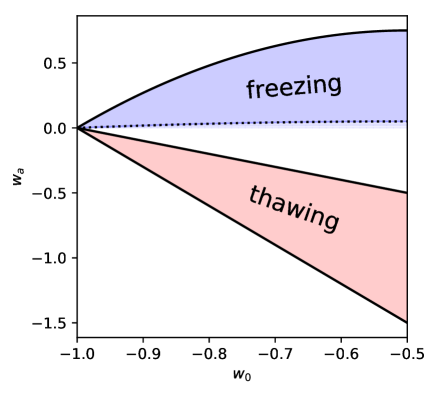
Figure 1: A schematic of the loci of freezing and thawing models on the ($w_{0}$, $w_{a}$) plane.

Whether the quintessence field is in the freezing or thawing regime not only depends on the form of the potential but also depends heavily on the initial conditions one is considering. Furthermore, it is possible to choose potentials such that the intermediate and late time behaviour is an attractor, independent of initial conditions. Models endowed with this behaviour are known as tracker models. In practice, and without tracking, natural initial conditions inevitably lead to thawing behaviour (as we will discuss in Section III) and, in this paper, we will focus on characterizing these models thoroughly.

In this paper we will consider a comprehensive suite of dark energy models (see Copeland et al. (2006); Tsujikawa (2013) for a broad range). Building on the choices of Marsh et al. (2014) we will explore and characterize the following subclasses of thawing potentials given by Eq. 10 and represented in Table 1:
Monomial: $V\sim\phi^{N}$; $N$ can be positive, such as the case of a massive Klein-Gordon field $(N=2)$ or a scale-invariant field $(N=4)$; or negative. Both cases lead to thawing behavior, provided one solves the evolution equation from early times. It has been argued that a negative $N$ would lead to freezing behaviour Caldwell and Linder (2005); Barger et al. (2006); however, this is only true if the initial conditions are set at low redshift (see Fig. 2) or the kinetic energy is similar to the potential energy at the origin and $V(\phi_{i})\gg V(\phi_{0})$ (see discussion in next Section). In general, starting from deep inside the radiation epoch, the Hubble parameter is large ($\ddot{\phi}+3\dot{\phi}H\approx 0$) and freezes the field ($\dot{\phi}=\dot{\phi}_{i}a^{-3}$), which only starts evolving at late times (thawing). In addition, the early dark energy constraints from CMB and Big-Bang Nucleosynthesis (BBN) ($\sim 1\%$ Ade et al. (2014, 2016a)), limits the maximum value of $\dot{\phi}_{i}$. Recall that, during kination, $\rho_{DE}\sim\dot{\phi}^{2}=\dot{\phi}_{i}^{2}a^{-6}$.
Effective Field Theory (EFT): $V$ is sum of monomials suitably weighted by the corrected powers of a mass scale consistent with the view that it arises as a consistent low energy limit of a theory. This series represents corrections from operators representing high-energy physics. The series converges if the parameter $\varepsilon_{\rm F}$ is small, required by the super-Planckian shift symmetry that imposes $\varepsilon_{F}<1$. We will call $n_{Q}$ to the number of quantum corrections.
Modulus: $V\sim\epsilon_{D}^{n}e^{\lambda_{n}\phi}$; the vacua potential of theories with higher order dimensions are usually proportional to exponentials of the field Copeland et al. (2006). We consider here weighted sums of them, where $\epsilon_{D}$ is the compactification scale. In addition, we parametrize $\lambda_{n}=\alpha(p_{D}-n)$, so that $\lambda_{n}$ can be positive or negative, depending on the order of the term, and weighted by $\alpha$.
Axion: $V\sim 1+\cos(\epsilon_{\mathrm{F}}\phi)$ where $\epsilon_{\mathrm{F}}$ is related to the symmetry breaking scale; these potential arise in theories where the field is a pseudo-nambu Goldstone boson. Note that we are interested in a regime different of that in which axions contribute to dark matter, in which the field oscillates around a minimum of the potential and the equation of state averages to zero.

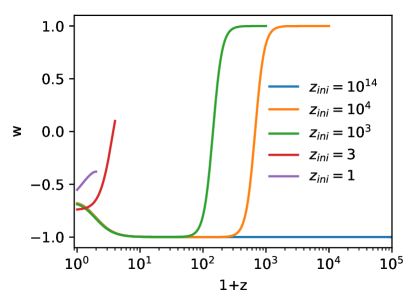
Figure 2: Effect of the initial conditions on the dynamics of the model $U\propto\phi^{-2}$ with initial conditions $\phi_{i}=M_{P}$ and $\phi^{\prime}_{i}\equiv\mathrm{d}\phi/\mathrm{d}\tau|_{i}=H_{0}$. Just starting the integration close enough $z=0$ the initial velocity of the field can survive and yield a freezing behavior.

Model	$b_{n}(\phi)$	$c_{n}$	$n_{\rm min}$	$f(\phi)$	$\phi_{i}$
Monomial	0	–	–	$\phi^{N}$	$[1,7]$
EFT	$\phi^{n}$	$(\epsilon_{\mathrm{F}})^{n}$	$p_{E}$	$\sum\limits_{i=2,4}\xi_{i}(\epsilon_{\rm F}\phi)^{i}$	$[1,10]_{\log_{10}}$
Modulus	$e^{\alpha(p_{D}-n)\phi}$	$(\epsilon_{D})^{n}$	0	0	$[-1,1]$
Axion	$\cos(n\epsilon_{\mathrm{F}}\phi)$	$(\epsilon_{\mathrm{NP}})^{n-1}$	$2$	$1+\cos\epsilon_{\rm F}\phi$	$~{}[-\frac{\pi}{\epsilon_{\rm F}},\frac{\pi}{\epsilon_{\rm F}}]~{}$

Table 1: Elements of the potential (Eq. 10) for the studied models. Note that for EFT, $\phi_{i}\in[1,10]_{\log_{10}}$ stands for $\log_{10}(\phi_{i})\in[0,1]$.

III Establishing Physical Priors

Before we attempt to construct an efficient and comprehensive parametrization of quintessence models it is useful to explore the broad characteristics one might expect if one focuses on what we determine to be physical priors. We will focus on ($w_{0}$, $w_{a}$), very much along the lines of Caldwell and Linder (2005); Barger et al. (2006); Huterer and Peiris (2007); Marsh et al. (2014). This will allow us to explain and make explicit our choices that then lead to a distribution of dynamical behaviours for each individual model.

We can split the choices into a) cosmological parameters that affect that background evolution b) parameters in the action (or more specifically, the potential $V(\phi)$ and c) initial conditions for the scalar field. With regards to a) we chose to be sufficiently general but not overly so, or the analysis is impractical. This means that we choose to vary cosmological parameters that most directly affect the background evolution and which play off against the scalar field evolution. Specifically, we restrict ourselves to just $h$ (where the Hubble constant is $H_{0}=100\,h\,\mathrm{km\,s^{-1}Mpc^{-1}}$) and the fractional density of cold dark matter today, $\Omega_{cdm}$; We choose the ranges $h\in U[0.6,0.8]$ and $\Omega_{cdm}\in U[0.15,0.34]$. It is important to note that ranges are chosen to be broad enough so that we do not bias our result, but we do not explore regimes that are clearly ruled out by current observations (e.g. $H_{0}=0$) . In particular, $\Omega_{cdm}$ priors might seem too broad in comparison with typical constraints. However, they were enlarged to allow for compatible results with tomographic weak lensing constraints from KiDS-450 Hildebrandt et al. (2017) or CFHTLenS Joudaki et al. (2017), which gave weaker constraints on $\Omega_{m}$.

With regards to parameters in the potential, the choices are more subtle. In principle one should work within the framework of effective field theory and only include terms (“operators”) with a suitable dimensionfull weighting and dimensionless parameters of $O(1)$. Indeed, one of the options makes this philosophy explicit – the case of EFT – and generally we obey this principle. Nevertheless, if used bluntly, this can severely restrict the range of behaviours; indeed it will be overwhelming dominated by a cosmological constant. We take care to allow for more general behaviour to be able to emerge.

We should note that alternatives are permissible where naturalness still plays a role (e.g. in the case of monomial potentials that break shift symmetry) or where other symmetry principles may be at play (as in the case of scale invariant potentials or axion like potentials). Furthermore, more complex operators arising from the low energy limit of higher dimensional theories and their variants (where, for example, factors of $e^{\lambda\phi}$ might emerge) are also considered.

Finally, we need to address the initial conditions for the scalar field. We assume that the initial conditions are established deep in the radiation era and there we can identify two different regimes. In the first case, the expansion of the Universe will have damped the evolution such that, in full generality, ${\dot{\phi}}=0$. We can, again, use the view point of effective field theory and assume that the amplitude of the scalar field is of a $O(1)$ in terms of either Planck units or the fiducial mass scale which is used for dimensionful power counting. Alternatively, one can assume that the scalar field “scales” or “tracks” initially, i.e. that its background energy density follows that of radiation. In that case the initial value and velocity is uniquely determined by the background cosmology.

We have chosen these ranges in cosmological and potential parameters as well as in the initial conditions for the scalar field to span as broad a set of possibilities as are physically credible, very much in the spirit of Marsh et al. (2014). A list of the ranges is presented in Table 2 where the parameters are described in Section II. This does mean that we are excluding what we consider unphysical possibilities such as, for example, starting the scalar field with an arbitrary velocity at some low redshift – there is simply no physical mechanism that would put it there. Or, for example, we do not consider hugely disparate sets of parameters in the potential, as the small parameters would receive large radiative corrections in the absence of a symmetry protecting them.

We also avoid having too many higher order terms in the potential, controlled by $n_{max}$ and $n_{Q}$, as that would make their contribution negligible. In the same way we don’t have either too low or too high values of the weighting constants $\epsilon_{F,NP,D}$ that would make the higher order terms either stop contributing or explode. Similarly, we choose $\alpha$ and $p_{D}$ priors for Modulus so that the exponent size is controlled, despite allowing for unlikely large values such as $e^{5}$. For the monomial case, large $N$ values would make the potential too steep making the field evolve too fast and yielding unphysical or highly tuned results. Finally, the $\xi_{n}$ constants weigh randomly higher order term in the potential, leading us to take their values from a Normal distribution.

Parameter	Model	Distribution
$A$	All	Fixed by $1=\sum_{i}\Omega_{i}$
$\xi_{n}$	All	$\mathcal{N}(0,1)$
$N$	Monomial	$\mathrm{U}_{\mathbb{Z}}[1,7)$
$n_{\rm max}$	Modulus, Axion	$\mathrm{U}_{\mathbb{Z}}[10,20]$
$n_{\rm Q}$, $p_{E}$	EFT	$\mathrm{U}_{\mathbb{Z}}[5,10]$
$\log_{10}\epsilon_{\rm F,NP,D}$	EFT, Modulus, Axion	$\mathrm{U}[-3,-1)$
$p_{D}$	Modulus	$\mathrm{U}_{\mathbb{Z}}[1,5]$
$\alpha$	Modulus	$\mathrm{U}[0,1]$

Table 2: Parameters distributions. $\mathrm{U}[a,b]$ stands for the uniform distribution between $a$ and $b$ and $\mathrm{U}_{\mathbb{Z}}$ is the uniform distribution in the integers.

In Fig. 3 we can get an idea of the dominant type of behaviour for the class of models we consider, in terms of the equation of state. Focusing, for now, on the solid contours, we can see that these models lead exclusively to thawing models. The only way to change this behaviour (unless the potential tracks the dominant energy density) is to give the scalar field large initial velocities at late time (see Fig. 2); these are completely unphysical as they correspond to unacceptable velocities in the radiation era – i.e. there is no physical mechanism for achieving these velocities and hence, such evolution cannot be, in any way considered part of a set of physical priors. We note that, in the analysis of Huterer and Peiris (2007) such unphysical initial conditions were considered by starting the integration of the background at late redshifts ($z=3$). This prevents the expansion of the universe to dilute the initial conditions and hence the unnatural prevalence of freezing models in their analysis. We also note that this plot pretty much reflects the findings of Marsh et al. (2014).

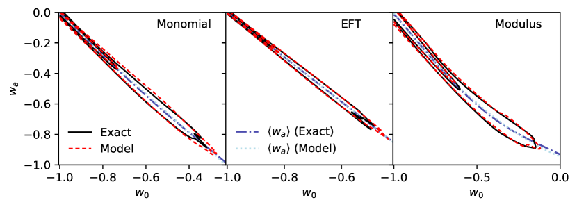
Figure 3: $w_{0}$-$w_{a}$ distributions for the Monomial (left panel), EFT (central panel) and Modulus (right panel). All these models have $w_{a}\neq 0$, while Axion can be described just with $w_{0}\leq-1+10^{-4}$ (95% C.L.). In this Figure we are comparing the prior distributions found for $w_{0}$-$w_{a}$ fitting the observables (the Exact); i.e. minimizing Eq. 17; and the distributions obtained with our analytic approximation (Model), i.e. with Eq. 18-21.

Freezing models can be obtained in at least two situations. In tracker models, solutions exist in which the quintessence energy density is a fraction of the dominant matter component, e.g. radiation at early times. This early dark energy contributes to the expansion rate throughout cosmic history and is thus subject to constraints from CMB and BBN Ade et al. (2016a). Generic initial conditions will cause the field to be frozen at $\rho_{\rm DE}\sim V(\phi_{i})$, entering the tracking behavior when $V\sim\rho$. A tracking behaviour at all epochs can be achieved through an exponential potential, although a change on $V_{,\phi}/V$ is necessary for the field to freeze in Copeland et al. (1998); Barreiro et al. (2000). Other freezing models can be obtained with inverse power-law potential (i.e. monomial with $N<0$) Ng et al. (2001); de la Macorra and Piccinelli (2000). In this case the field evolves with a fixed equation of state, rather than track the dominant matter component. However such a simple potential does not successfully freeze to $w\sim-1$ at low redshift unless $N$ is close to zero, effectively recovering the cosmological constant behaviour, cf. Fig. 4. In both cases, freezing behaviour requires that the initial conditions for the field are so that $V(\phi_{i})\gg V(\phi_{0})$ ($\rho_{\rm DE}(\phi_{i})\gg\rho_{\rm DE}(\phi_{0})$) – only thawing behavior can occur if the initial energy density of quintessence is small, as it is the case for the priors used here. Neither purely exponential or inverse power-law potentials can act as viable freezing models – we will leave the study of other potentials with freezing behavior for a future study.

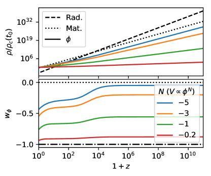
Figure 4: Freezing behavior for inverse power-law potentials (monomial quintessence $N<0$). Freezing behavior is possible if the energy density of the field is significant at early times $V(\phi_{i})\gg V(\phi_{0})$ (upper panel). However, in order to achieve $w(z=0)\approx-1$ the potential needs to be very flat ($N\approx 0$), a requirement that pushes the model towards a $\Lambda$ limit (lower panel).

IV Parameterizing quintessence

We now proceed to describe the method by which we compress information about the quintessence component in such a way as to retain as much information as necessary for a reliable model comparison or likelihood analysis. In this paper, as it is customary, we choose to work with the equation of state $w$, which enters into the equations of the observables through the energy density:

$$\rho_{\rm DE}=\rho_{\rm DE}^{(0)}\exp\left[-3\int_{0}^{log(a)}dlog(a^{\prime})[1+w(a^{\prime})]\right]\,.$$ (15)

The Hubble rate, $H$, and the angular diameter distance, $D_{A}$, only depend on the energy densities:

$$H^{2} \propto\sum_{i}\rho_{i}\,,$$

$$D_{A} =\int_{0}^{z}\frac{dz^{\prime}}{H(z)}\,,$$

while the growth rate of structure, $f=d\ln\delta_{M}/d\ln a$ (where $\delta_{M}$ is the matter density contrast) also depends (mildly) on $w$:

$$(1+z)\frac{df}{dz} =\frac{1}{2}\left(1-\sum_{i}\frac{3w_{i}\rho_{i}}{H^{2}}\right)f+f^{2}-\frac{3}{2}\Omega_{M}(z)\,.$$

In choosing a parametrisation, one has to assess how well it approximates the dynamics it is supposed to represent. To do so, one needs some kind of measure. For example, it should be good enough that evolution of distinct classes of models, once parameterised, are easily distinguishable. In practice this means one needs to construct realisations of this evolution (the equation of state, $w$, in this case) from a realistic priors for a particular class of models and check that the parametrisation follows these realisations faithfully and in such a way that it is clearly distinguishable from another class of models.

There is also a practical guide that guides the quality of the parametrisation. Ultimately we will use it to generate mock observables that will be compared to data. We are looking forward and assuming that the quality of the data will be such that we will have, at most, percent errors on the observables. This means that we should aim to have a parametrisation which is accurate at the sub-percent level but not much more. Another way of stating it is that the systematic errors arising from our modelling of the dark energy evolution (through the parametrisation) should be of the same order as (or marginally smaller than) the statistical and systematic errors arising from the observations themselves.

We will use the latter criteria as a practical guide in determining the quality of our parametrisation. The observables we will focus on are the angular diameter distance, $D_{A}(z)$, the growth rate, $f(z)$, and the Hubble parameter, over the range of redshifts which will be covered by the next generation of data sets. This is key (and a novel aspect) of the approach in this paper.

Our starting point is a finite series expansion of $w$,

$$w=\sum\limits_{m=0}^{M}c_{m}(1-a)^{m}\,,$$ (16)

Note this parametrization does not break at high order and that higher terms contribute more at early times ($a\rightarrow 0$). It will be convenient to denote ${\bf c}=(c_{1},c_{2},\cdots,c_{m})$.

While it is clear that the larger the number of coefficients (i.e the larger the $M$), the more accurate the parametrisation, we, naturally, want to come up with the most economical parametrization. Even though the equation of state can have a difficult evolution, the results of Marsh et al. (2014) and the fact that it will only be relevant when dark energy is not negligible, lead us to believe that it should, universally, be described by a combination of a few smooth functions. We shall see that, for thawing models of quintessence, which is the focus of this paper, the parametrization of Eq. 2 is sufficient. This means we need to find a probabality distribution function for $(w_{0},w_{a})$, ${\cal P}[w_{0},w_{a}]$ .

Our approach is as follows . For each class of theories, we generate a large number of possible evolutions for $w$, using the approach described in Section III. We work with hi_class Zumalacárregui et al. (2017); Bellini et al. (2019), a modified version of the Boltzmann code CLASS Blas et al. (2011) that incorporates Horndeski theories Horndeski (1974); Deffayet et al. (2011); Kobayashi et al. (2011), to solve the cosmological equations and obtain the exact observables for each realization. In addition, the parameters of the model must be chosen so that we are able to reproduce the phenomenology of the given model, with mild restrictions based on stability and more fundamental physics. Given an ensemble of models, parameters are obtained fitting $w_{0}$ and $w_{a}$ so that they minimize the error on the observables at specific redshifts; i.e. minimizing

$$\chi^{2}=\sum_{i}\frac{(\mathcal{O}({\vec{c}})-\mathcal{O}(\phi))_{i}^{2}}{\sigma_{\mathcal{O}_{i}}^{2}}\,,$$ (17)

where $\mathcal{O}(\phi)_{i}$ stands for the exact $D_{A}$, $H$ and $f$ at the specific redshift $z_{i}$, computed solving the field equation and, therefore, depends on the specific choice of the model parameters in Table 1. On the other hand, $\mathcal{O}(\vec{c})$ stands for the observables computed using the parametrized $w$. As we will see, $\mathcal{O}(\vec{c})\equiv\mathcal{O}(w_{0},w_{a})$. Finally, $\sigma_{\mathcal{O}_{i}}$ is the desired precision, which, in all cases, we choose it to be lower than $1\%$ at low redshift (i.e. $z<z_{low}=10$) Abell et al. (2009); Font-Ribera et al. (2014); Aghamousa et al. (2016), and $0.3\%$ at recombination for $D_{A}$ Joudaki et al. (2018). Note that, using the parametrization it is possible that $w$ crosses $w=-1$. To allow for such models that, however, reproduce the observables accurately, we use the fluid equations with the Parametrized post-Friedmann (PPF) approximation Fang et al. (2008), already implemented in CLASS.

Equation 17 neglects the fact that the observables are, in general, correlated. However, we can safely disregard this contribution as Eq. 17 suffices to achieve the goal precision. This will be seen in following Section.

With this machinery in hand, we can study the probability distribution functions (PDFs) of $(w_{0},w_{a})$ and from them we are able to generate the PDFs for the observables, $D_{A}$, $H$ and $f$.

V Results

We now proceed to construct a distribution function for $w_{0}$ and $w_{a}$. To begin with, we generate ensembles of cosmologies for each of the models. We follow the procedure we discussed in Section III to generate $20,000$ realizations for each class of models, which we have seen is enough to produce stable results. Given the extra accuracy we need for $D_{A}(z_{rec})$, we weight the low redshift observables with $\sigma_{\mathcal{O}_{i}}=10^{-3}$ and $\sigma_{D_{A}(z_{rec})}=10^{-4}$ for the angular diameter distance point at recombination in Eq. 17. Do not confuse these variables with the maximum allowed errors. They are set lower to ensure the maximum errors are below our threshold (i.e. 1% at low redshift and 0.3% for $D_{A}(z_{rec})$).

Revisiting Fig. 3, we note that the contours for $(w_{0},w_{a})$ all have similar characteristics: a long degeneracy direction (given by the dotted line) towards the bottom right while a reasonable tight distribution along the (quasi)-orthogonal direction. This is characteristic of thawing models, as has been previously observed in Marsh et al. (2014); Linder (2015). In the end, the field evolution for thawing models is just a slow (to be physically viable) roll down of the potential and, consequently, produces similar effects. We will exploit this structure further down.

To begin with, as explained before, we check the quality of this parametrization by generating our proxies for the observables, now with $(w_{0},w_{a})$ and comparing, model by model, with the original full calculation. In Fig. 5 we can see that, apart from a very few outliers, most models lie well within our target precision. In other words, using $(w_{0},w_{a})$ we generate observables which agree with those calculated from the full evolution to better than our threshold. This gives us confidence that describing $w(a)$ in terms of two parameters is good enough for any of the planned surveys.

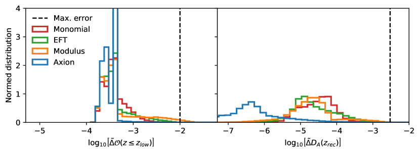
Figure 5: Distribution of the maximum relative error of the observables for each Quintessence model compared to its fit in the $(w_{0},\,w_{a})$ plane, i.e. $\tilde{\Delta}\mathcal{O}\equiv\left|\mathcal{O}({\rm Fit})/\mathcal{O}({\rm Quintessence})-1\right|$. In the left panel $\mathcal{O}$ stands for any observable among $H$, $f$ or $D_{A}$, whichever gives the maximum error at low redshift ($z<z_{low}=10$). In the right panel we show the maximum error at recombination for the angular diameter distance $D_{A}(z_{rec})$.

It is interesting to see how well the parametrized $w(a)$ approximates the full one as a function of redshift. In Fig. 6 we plot the maximum deviation between the two. We can see that for $z>1$, the differences are appreciable. This is, of course, to be expected. The dark energy density at those redshift is sufficiently subdominant and will contribute very little to the observables.

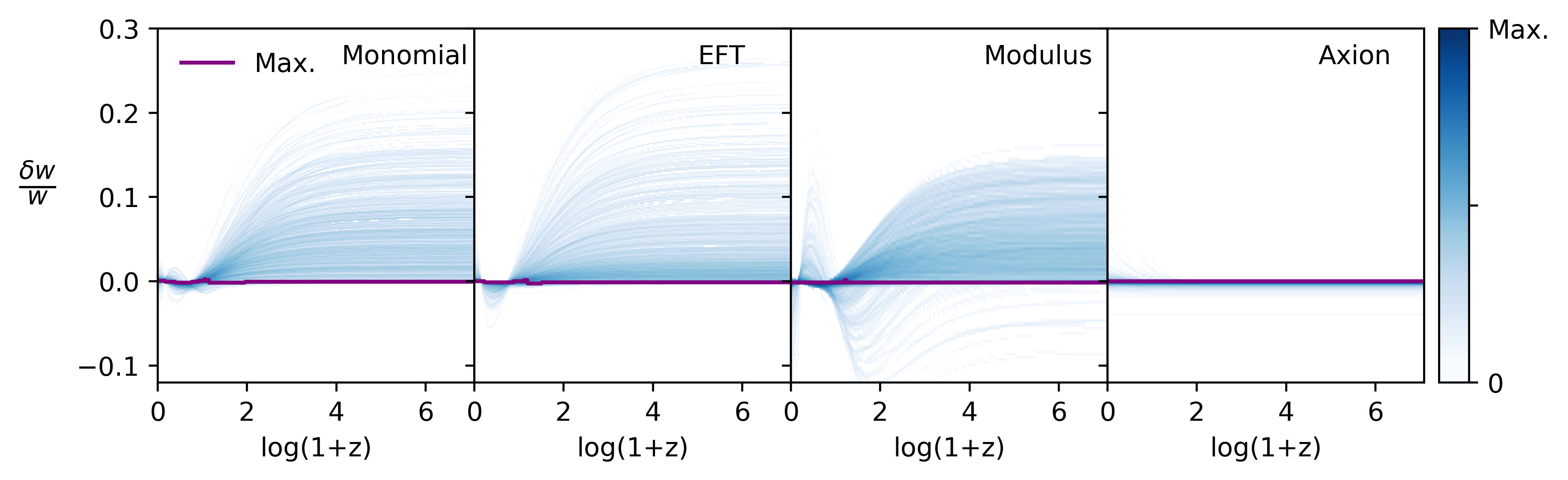
Figure 6: Density plots, one for each Quintessence model, showing the time evolution of the relative difference between $w(a)$ obtained from the original realization and after fitting it in the $(w_{0},\,w_{a})$ plane. Darker colors indicate the presence of more models with that particular relative difference at that redshift. The purple lines show the maximum density for each model.

With the distributions in hand for $(w_{0},w_{a})$ we can construct an analytic model. We assume that the distribution can be factorized into

$${\cal P}[w_{0},w_{a}]={\cal P}[w_{a}|w_{0}]{\cal P}[w_{0}]\,.$$ (18)

We can see in Fig. 7, the ${\cal P}[w_{0}]$ for each model (solid line) is sharply peaked at $w_{0}=-1$. While an exponential is a reasonable approximation, we find that

$${\cal P}[w_{0}]=A_{1}e^{-\left(\frac{w_{0}}{w_{1}}\right)^{\alpha_{1}}}+A_{2}e^{-\left(\frac{w_{0}}{w_{2}}\right)^{\alpha_{2}}}$$ (19)

is more robust and can cover more models. In Fig. 7 we see that approximate form as a dashed line.

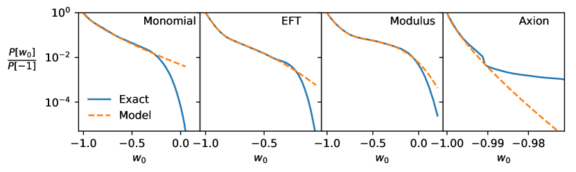
Figure 7: For each model, we show the exact (blue solid lines) probability distribution of $w_{0}$ normalized to 1 for $w_{0}=-1$. The approximate analytic model defined in Eq. 19 is also shown (orange dashed lines). It is possible to appreciate the excellent agreement between the two curves down to probabilities of $10^{-2}$, which includes the region preferred by the data in most models.

From the contour plots in Fig. 3 we can also see that there is a well defined degeneracy direction in $(w_{0},w_{a})$ (the dotted lines). The degeneracy line, ${\bar{w}}_{a}(w_{0})$ is well approximated by a quadratic

$$\bar{w}_{a}(w_{0})\simeq\beta_{0}+\beta_{1}w_{0}+\beta_{2}w_{0}^{2}\,.$$ (20)

We now want to look at the conditional probability, ${\cal P}[w_{a}|w_{0}]$. From Fig. 8 we can see that, for each value of $w_{0}$, the distribution is peaked around $\bar{w}_{a}(w_{0})$ and well approximated by a Gaussian. We thus use the ansatz

$${\cal P}[w_{a}|w_{0}]=\frac{1}{\sqrt{2\pi\sigma^{2}(w_{0})}}e^{-\left(\frac{w_{a}-\bar{w_{a}}(w_{0})}{2\sigma(w_{0})}\right)^{2}}\,,$$ (21)

where the variance is given by

$$\sigma(w_{0})\simeq\sigma_{0}+\sigma_{1}w_{0}+\sigma_{2}w_{0}^{2}\,.$$ (22)

The fits to these parameters for each class of models are given in tables 3 and 4, respectively. Although they are given with high accuracy, we have found that small changes do not affect the $w_{0}$-$w_{a}$ distribution and, specially, the distributions of the observables. Nevertheless, we are cautious and use three significant figures. The study of the minimum required accuracy goes beyond the scope of this work.

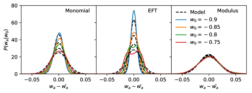
Figure 8: For each model, Axion excluded since it can be parametrized solely in terms of $w_{0}$, we show the conditional probability distribution of $w_{a}$ given specific values of $w_{0}$ (colored solid lines). Dashed black lines represent the same curves obtained using our analytic approximation, Eq. 21. The parameters of this equation have been obtained through a global fitting. This explains the discrepancy between the solid and dashed curves, but it does not affect the observables as shown in Fig. 9.

Model	$A_{1}$	$w_{1}$	$\alpha_{1}$	$A_{2}$	$w_{2}$	$\alpha_{2}$
Axion	737	0.775	$-1.08\times 10^{-3}$	0	-	-
Monomial	8.21	0.734	0.102	0	-	-
EFT	12.9	1.01	0.0499	1.05	1.76	0.383
Modulus	8.13	0.890	0.0712	0.535	3.95	0.803

Table 3: Fit parameters for ${\cal P}[w_{0}]$ (Eq. 19) model distributions

.

Model	$\beta_{0}$	$\beta_{1}$	$\beta_{2}$	$\sigma_{0}$	$\sigma_{1}$	$\sigma_{2}$
Monomial	-1.28	-1.21	0.0564	0.0769	0.108	0.0357
EFT	-1.43	-1.35	0.0882	0.0556	0.0577	0.00320
Modulus	-0.946	-0.460	0.481	0.0755	0.121	0.0628

Table 4: Fit parameters for ${\cal P}[w_{a}|w_{0}]$ (Eq. 21) model distributions. Recall that $\langle w_{a}\rangle(w_{0},\,\beta_{i})$ and $\sigma(w_{0},\,\sigma_{i})$ are given by Eqs. 20 and 22, respectively.

.

We can now revisit the contour plots, comparing the original ones with those from our analytical model. In Fig. 3 we overlay the two sets and, unsurprisingly, find very close agreement. The final step is now to sample from the analytic priors to generate the observables and compare them with those generated by the full scalar field evolution. In Fig. 9 we overlay the contours for the case with the largest differences, i.e. for the Modulus model at redshift $z=1$. We find an excellent agreement between the two, giving us confidence that the analytic priors can be used as reasonably accurate representation of the quintessence space in future cosmological analysis. It must be noted that we checked the truth of this statement for all models at different redshifts ($z=0.1,\,0.5,\,1.0,\,2.0,\,5.0,\mbox{ and }10$). In section VI, we will study the impact of these analytic priors when used in combination with actual data and see that they considerably increase the constraining power of the data.

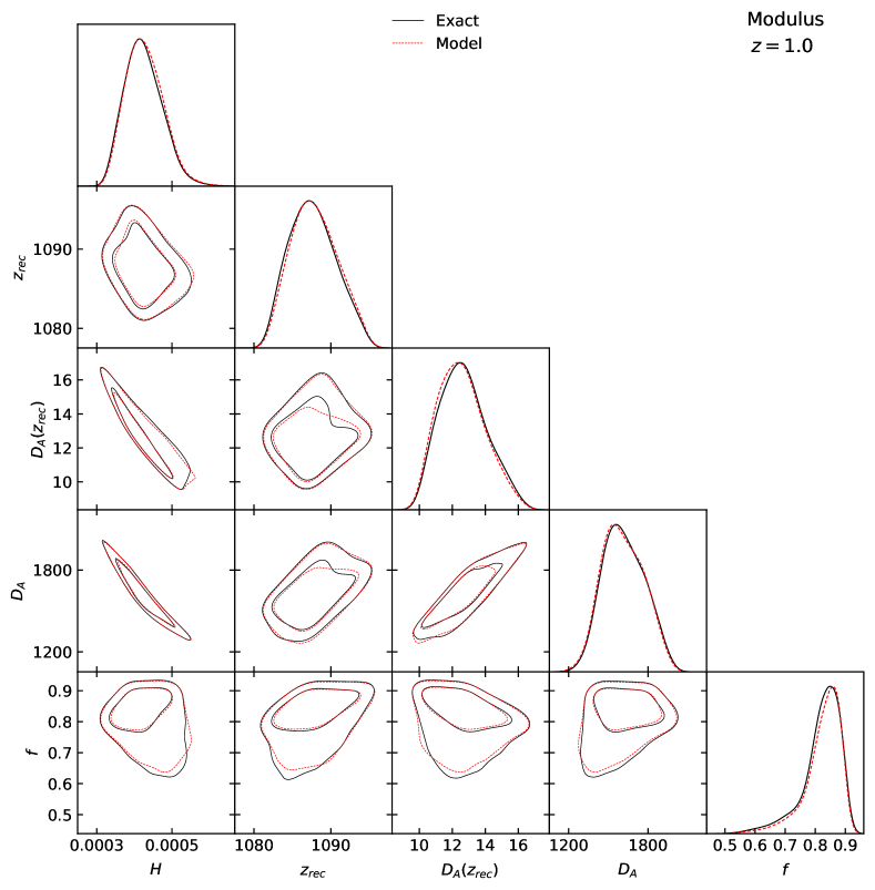
Figure 9: Distributions of the observables obtained integrating the field equations of motion (solid black line) compared to those obtained sampling from our parametrization. These are the results for modulus at redshift $z=1$, which was the case we found largest differences. However, they are small and will have little impact when the analytic expressions are used in combination with data.

In general, the analytic expression are stable under changes of the parameters’ priors. We checked the stability of the results by approximately doubling or halving the width of the prior distributions and saw that, even though (in a very few cases) the actual numbers change, the new distributions can be still parametrized by Eqs. 19 and 21. In particular, we saw that Monomial and EFT distributions remain unchanged, while the distributions for Axion and, more significantly, Modulus varied. The exponential potential of Modulus makes it more sensitive to changes on the field.

In the following lines we summarize some key, individual, features of each model.
Monomial: The two parameters, $w_{0}$-$w_{a}$, suffice to reproduce the observables accurately. In fact, minimizing the $\chi^{2}$ with the observables (Eq. 17) yields equivalent distributions to those obtained fitting the actual curves (i.e. $w$) at low redshift. The probability distribution of $w_{0}$, $P[w_{0}]$, is correctly reproduced with just one of the exponentials in Eq. 19. The parametrized $w$ goes to lower values than the original one, meaning that, for a large fraction of the models, one needs $w<-1$ at early times to effectively recover the model.
EFT: The two parameters, $w_{0}$-$w_{a}$, suffice to reproduce the observables accurately. In contrast with the monomial case, fitting $w$ at low redshift yields different distributions for the parameters. This is consequence of faster evolutions of the field close to $z=0$. In addition, our prior on $\phi_{i}$ substantially enlarge the $w_{0}$-$w_{a}$ distribution in comparison with that in Marsh et al. (2014). This is consequence of having initial values of the field considerably lower than $1/\epsilon_{F}$ and forcing the Friedmann equation to hold today. While in Marsh et al. (2014) $\phi_{i}\in[-1/\epsilon_{F},1/\epsilon_{F}]$ (with $\log_{10}(\epsilon_{F})\in[-3,-1]$), we imposed a fixed range $\phi_{i}\in[1,10]$; the smaller $(\epsilon_{F}\phi)^{n}$ terms that enter into the potential, force the potential to be (substantially) larger, leading to a large derivative, $V_{,\phi}$.
Modulus: The two parameters, $w_{0}$-$w_{a}$, suffice to reproduce the observables accurately. The more complicated dynamics are reflected in both the fit performance and the way $w$ is recovered in comparison with the original: the errors on the observables, although good enough, have longer tails relative to other models; in addition, in contrast with previous cases, many models have $w(w_{0},w_{a})>w(z)$ at early times.
Axion: Just one parameter is needed to reproduce the observables accurately: $w_{0}$. In this case, the field remains frozen for almost all its history and just starts moving very close to the present. As in the previous case, $w(w_{0})>w(z)$ at early times, in a form that compensates the (small) late time evolution of the field, but does not change the early universe dynamics.

VI Comparison with current data

In this section we present the constraints on the equation of state from current cosmological data and combine them with the analytical priors of previous section. Let us briefly go through the method. We do a Bayesian analysis, sampling through $w_{0}$ and $w_{a}$ along with the standard cosmological parameters in a Markov Chain Monte Carlo (MCMC) with MontePython Audren et al. (2013); Brinckmann and Lesgourgues (2018) using the Metropolis-Hastings algorithm Metropolis et al. (1953); Hastings (1970). We have used the Gelman-Rubin convergence criterion Gelman and Rubin (1992), requiring $R-1<0.01$.

We have used the following datasets:
CMB: From Planck 2015 Adam et al. (2016); Ade et al. (2016b); Aghanim et al. (2016), we use the high $l$ temperature autocorrelation (TT) likelihood, in the range $l=30-2508$, along with the likelihood of the joint autocorrelations of the temperature (TT), the E and B polarization modes (EE and BB) and the cross-correlation of the temperature with the E-polarization mode (TE) for $l=2-29$ and the lensing likelihood (with temperature and polarisation lensing reconstruction) in the multipole range $l=40-400$.
BAO: We use Baryon Acoustic Oscillation (BAO) measurements from 6dFGS survey Beutler et al. (2011), the Sloan Digital Sky Survey (SDSS) DR7 Main Galaxy Sample (MGS) Ross et al. (2015), and BOSS DR12 Alam et al. (2017). The first two measure the expansion history through the redshift-distance and redshift-Hubble relations combined through the relation, $D_{\rm V}=(D_{\rm A}^{2}(1+z)^{2}z/H)^{1/3}$, where $D_{\rm V}$ is the angle-averaged distance, $D_{\rm A}$ - the angular diameter distance and $z$ is the redshift BOSS DR12 constrains both the angular diameter distance, $D_{\rm A}$ and the Hubble parameter, $H$. We do not consider the correlation between the BOSS measurements and the 6dF and MGS survey as those surveys cover different patches of the sky and hence any such correlation would be negligible.
RSD: We use Redshift Space Distortions (RSD) measurements derived form from 6dFGS Beutler et al. (2012) and BOSS DR12 Alam et al. (2017), where for BOSS we use the full covariance between the 3 $f(z)\sigma_{8}(z)$ measurements at different redshifts and the BAO measurements of $H(z)$ and $D_{\rm A}(z)$.
SNe Ia: We use the new Pantheon Supernovae (SNe) Ia sample Scolnic et al. (2018), which combines observations from the Pan-STARRS1 Medium Deep Surveyat redshift $0.03<z<0.65$ with ones from the SDSS, SuperNova Legacy Survey (SNLS), and various low-redshift and HST samples. In total 1048 SNe Ia in the redshift range $0.01<z<2.3$.

We note that, throughout, we assume that the cross-correlation between the different datasets is negligible. To obtain the combined constraints from data and theory we implemented the priors as a likelihood module in MontePython and plotted the results with the python package for analysing MCMC samples GetDist Lewis (2019).

We begin by showing the results of a likelihood analysis without including our model for the theoretical priors in the left hand panel Fig. 10. The likelihood analysis with uniform priors on the equation of state parameters prefers a distinct direction in the $(w_{0},w_{a})$ plane which, interestingly, is not colinear with the ${\bar{w}}_{a}(w_{0})$ we derived in the previous section; this is clear from the overlay of the theoretical priors (and was already apparent in Marsh et al. (2014)). The Axion model, as has been repeatedly mentioned, is a special case, with an equation of state which is very concentrated at $w_{0}=-1$. For this model, we compare the widths of the posterior from the likelihood analysis with uniform priors on $(w_{0},w_{a})$ with the theoretical priors studied in this paper; clearly the theoretical prior is much tighter than the posterior. As mentioned above, Fig. 10, to some extent, echoes similar plots used in contour plots for $(n_{S},r)$ for constraining the inflationary landscape. There one tends to plot inflationary “tracks” for specific models, overlaying the contours from a likelihood analysis assuming uniform priors for $(n_{S},r)$.

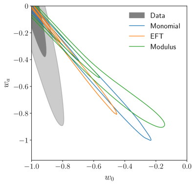
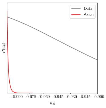
Figure 10: Distribution of $(w_{0},w_{a})$ for the CMB+BAO+RSD+SN combined datasets and the theoretical priors. On the left panel we show Monomial, Modulus and EFT and on the right panel Axion quintessence priors.

Even though the two sets of contours overlap, i.e. there is no ”tension” between them, we do not expect them to be aligned: very different physical considerations go into generating each set. Our choices were broad and uninformative in order to completely explore the phenomenology of the studied models. Furthermore the operational assumptions to build the analytical approximations of the PDF’s cannot bias our result as they almost perfectly recover the exact $w_{0}$-$w_{a}$ distributions.

If we invert the perspective and plot the theoretical priors individually and then incorporate them in the likelihood analysis of the current data, we see the power of combining the two. In the left hand side of Fig. 11, we can see a substantial reduction in the areas of the contours when the data is folded in. We see that the width of the likelihood contours of $(w_{0},w_{a})$ in the analysis that included the theoretical priors is a factor of few times smaller than for the theoretical priors alone. While one would expect the uncertainty in $(w_{0},w_{a})$ for the combination of priors and data to be substantially better than for an analysis with uniform priors and data, we can see how the non-colinearity of the prior and data contours works to our advantage and that, even with current data, combining with theoretical priors gives us greatly improved constraints.

To emphasize the power of including correct theoretical priors, in Table 5 we present constraints on $(w_{0},w_{a})$ for the likelihood analysis with uniform priors and with theoretical priors. Clearly there is a dramatic improvement in constraints. For completeness, again, we single out the case of the Axion model in the right hand panel of Fig. 11 to see that in this case the prior is so tightly centred at $w_{0}=-1$, combining it with data (also centred at $\sim-1$) does not improve the constraints significantly.

Data	$w_{0}=-1.012\pm 0.088$	$w_{a}=0.05\pm 0.36$
Data + Mono.	$w_{0}=-0.966\pm 0.027$	$w_{a}=-0.058\pm 0.036$
Data + EFT	$w_{0}=-0.968\pm 0.023$	$w_{a}=-0.040\pm 0.035$
Data + Mod.	$w_{0}=-0.967\pm 0.025$	$w_{a}=-0.054\pm 0.037$
Data + Axion	$w_{0}=-0.9983\pm 0.0020$	$w_{a}=0.0$

Table 5: Confidence limits of $w_{0}$ and $w_{a}$ for the combined data set CMB+BAO+RSD+SN (Data) and the data combined with the theoretical priors for each model.

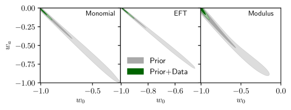
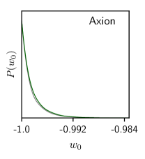
Figure 11: Constraints $(w_{0},w_{a})$ for the four different quintessence model from the CMB+BAO+RSD+SN combined datasets combined with the priors.

VII Discussion

In this paper we have proposed a simple, analytic model, for the priors of the equation of state, $w(a)$ of thawing quintessence. We have developed it for four specific thawing models but are confident it could be extended to any thawing model, given the observed similarities on the $(w_{0},w_{a})$ space Marsh et al. (2014); Linder (2015). It can now be used to either demarcate the physically allowed subset of the $(w_{0},w_{a})$ plane or incorporated into any future MCMC parameter estimation analysis. In Section VI we have trialled our proposal with existing data.

The prior for the equation of state factorizes easily into one probability distribution function for $w_{0}$ and another for $w_{a}$ conditional on the value of $w_{0}$. The model we propose is reasonably robust on the choice of fundamental parameters for each theory (i.e. fundamental constants in the quintessence action and initial values of the scalar field). We mean by this that the priors are unchanged when we vary these fundamental parameters or that the shape of the priors remains invariant (albeit with smaller or larger variances). We believe our choice of fundamental parameters is physical, erring on the conservative side. As a result, any future likelihood analysis is greatly simplified and it is no longer necessary to run the full scalar field dynamics to find the correct distribution of $(w_{0},w_{a})$.

One interesting, and important, consequence of having accurate physical priors is that, within the context of thawing models, constraints on $(w_{0},w_{a})$ are greatly improved. While this is not initially surprising – the physical priors we have characterized are much more restrictive than the usual uniform priors one uses for $(w_{0},w_{a})$ – the fact that the orientation of the prior distribution relative to that of the posterior constructed from the uniform prior with data also plays a key role. In fact, even though the posterior constructed from a uniform prior with data is much broader than the theoretical prior, the fact that they are not co-linear means that combining the two greatly improves the constraints on $(w_{0},w_{a})$ relative to the prior alone. As the data improves, we except this situation to be further exacerbated.

We have focused on thawing models but our approach must be extended to other models. Within the scope of quintessence, we have touched on tracker models which lead to freezing behaviour (we do not believe non-tracking, freezing models are physically realistic; these models need to be tuned so that $V(\phi_{i})\gg V(\phi_{0})$ and a sufficiently flat potential to correctly approximate to $w\sim-1$, as is exemplified in Fig. 4). Tracking models are not amenable to such a simple parametrization. One possible reason is due to the “quasi-nonanalyticity” of $w(a)$: in this case, the shape of the equation of state mimics that of rational functions which do not have well behaved Taylor expansions. Nevertheless, there may be alternative ways of parametrizing the equation of state (through, for example Pade approximants) that are amenable to the treatment here.

Naturally, we would like go beyond quintessence and we have tried to couch the task in as general way as possible, as a first step in completely characterizing Horndeski theories. For the case of quintessence, it has been an easy first step given that quintessence models have been extensively studied for over two decades and there is a detailed understanding of how the scalar field evolves in these scenarios. In the case of more general Horndeski theories, pockets have been studied well (such as Galileons or extended Jordan-Brans-Dicke theories) but a complete, generic framework for the scalar field evolution is still lacking. Only once such a framework is in hand can one start discussing physical priors for the parametrized versions of these theories, the ${\cal P}[{\vec{\alpha}}]$ discussed in the introduction.

References

- Riess et al. (1998) A. G. Riess et al. (Supernova Search Team), Astron. J. 116, 1009 (1998), arXiv:astro-ph/9805201 [astro-ph] .
- Perlmutter et al. (1999) S. Perlmutter et al. (Supernova Cosmology Project), Astrophys. J. 517, 565 (1999), arXiv:astro-ph/9812133 [astro-ph] .
- Abbott et al. (2019) T. M. C. Abbott et al. (DES), Astrophys. J. 872, L30 (2019), arXiv:1811.02374 [astro-ph.CO] .
- Hinshaw et al. (2013) G. Hinshaw et al. (WMAP), Astrophys. J. Suppl. 208, 19 (2013), arXiv:1212.5226 [astro-ph.CO] .
- Aghanim et al. (2018) N. Aghanim et al. (Planck), (2018), arXiv:1807.06209 [astro-ph.CO] .
- Alam et al. (2017) S. Alam et al. (BOSS), Mon. Not. Roy. Astron. Soc. 470, 2617 (2017), arXiv:1607.03155 [astro-ph.CO] .
- Abell et al. (2009) P. A. Abell et al. (LSST Science, LSST Project), (2009), arXiv:0912.0201 [astro-ph.IM] .
- Font-Ribera et al. (2014) A. Font-Ribera, P. McDonald, N. Mostek, B. A. Reid, H.-J. Seo, and A. Slosar, JCAP 1405, 023 (2014), arXiv:1308.4164 [astro-ph.CO] .
- Spergel et al. (2013) D. Spergel et al., (2013), arXiv:1305.5422 [astro-ph.IM] .
- Aghamousa et al. (2016) A. Aghamousa et al. (DESI), (2016), arXiv:1611.00036 [astro-ph.IM] .
- Hounsell et al. (2018) R. Hounsell et al., Astrophys. J. 867, 23 (2018), arXiv:1702.01747 [astro-ph.IM] .
- Caldwell et al. (1998) R. R. Caldwell, R. Dave, and P. J. Steinhardt, Phys. Rev. Lett. 80, 1582 (1998), arXiv:astro-ph/9708069 [astro-ph] .
- Lidsey et al. (1997) J. E. Lidsey, A. R. Liddle, E. W. Kolb, E. J. Copeland, T. Barreiro, and M. Abney, Rev. Mod. Phys. 69, 373 (1997), arXiv:astro-ph/9508078 [astro-ph] .
- Ratra and Peebles (1988) B. Ratra and P. J. E. Peebles, Phys. Rev. D37, 3406 (1988).
- Wetterich (1988) C. Wetterich, Nucl. Phys. B302, 668 (1988), arXiv:1711.03844 [hep-th] .
- Ferreira and Joyce (1998) P. G. Ferreira and M. Joyce, Phys. Rev. D58, 023503 (1998), arXiv:astro-ph/9711102 [astro-ph] .
- Copeland et al. (2006) E. J. Copeland, M. Sami, and S. Tsujikawa, Int. J. Mod. Phys. D15, 1753 (2006), arXiv:hep-th/0603057 [hep-th] .
- Tsujikawa (2013) S. Tsujikawa, Class. Quant. Grav. 30, 214003 (2013), arXiv:1304.1961 [gr-qc] .
- Marsh et al. (2014) D. J. E. Marsh, P. Bull, P. G. Ferreira, and A. Pontzen, Phys. Rev. D90, 105023 (2014), arXiv:1406.2301 [astro-ph.CO] .
- Raveri et al. (2017) M. Raveri, P. Bull, A. Silvestri, and L. Pogosian, Phys. Rev. D96, 083509 (2017), arXiv:1703.05297 [astro-ph.CO] .
- Gerardi et al. (2019) F. Gerardi, M. Martinelli, and A. Silvestri, JCAP 1907, 042 (2019), arXiv:1902.09423 [astro-ph.CO] .
- Chevallier and Polarski (2001) M. Chevallier and D. Polarski, Int. J. Mod. Phys. D10, 213 (2001), arXiv:gr-qc/0009008 [gr-qc] .
- Linder (2003) E. V. Linder, Phys. Rev. Lett. 90, 091301 (2003), arXiv:astro-ph/0208512 [astro-ph] .
- Sprenger et al. (2019) T. Sprenger, M. Archidiacono, T. Brinckmann, S. Clesse, and J. Lesgourgues, JCAP 1902, 047 (2019), arXiv:1801.08331 [astro-ph.CO] .
- Horndeski (1974) G. W. Horndeski, Int. J. Theor. Phys. 10, 363 (1974).
- Deffayet et al. (2011) C. Deffayet, X. Gao, D. A. Steer, and G. Zahariade, Phys. Rev. D84, 064039 (2011), arXiv:1103.3260 [hep-th] .
- Kobayashi et al. (2011) T. Kobayashi, M. Yamaguchi, and J. Yokoyama, Prog. Theor. Phys. 126, 511 (2011), arXiv:1105.5723 [hep-th] .
- Caldwell and Linder (2005) R. R. Caldwell and E. V. Linder, Phys. Rev. Lett. 95, 141301 (2005), arXiv:astro-ph/0505494 [astro-ph] .
- Barger et al. (2006) V. Barger, E. Guarnaccia, and D. Marfatia, Phys. Lett. B635, 61 (2006), arXiv:hep-ph/0512320 [hep-ph] .
- Ade et al. (2014) P. A. R. Ade et al. (Planck), Astron. Astrophys. 571, A16 (2014), arXiv:1303.5076 [astro-ph.CO] .
- Ade et al. (2016a) P. A. R. Ade et al. (Planck), Astron. Astrophys. 594, A14 (2016a), arXiv:1502.01590 [astro-ph.CO] .
- Huterer and Peiris (2007) D. Huterer and H. V. Peiris, Phys. Rev. D75, 083503 (2007), arXiv:astro-ph/0610427 [astro-ph] .
- Hildebrandt et al. (2017) H. Hildebrandt et al., Mon. Not. Roy. Astron. Soc. 465, 1454 (2017), arXiv:1606.05338 [astro-ph.CO] .
- Joudaki et al. (2017) S. Joudaki et al., Mon. Not. Roy. Astron. Soc. 465, 2033 (2017), arXiv:1601.05786 [astro-ph.CO] .
- Copeland et al. (1998) E. J. Copeland, A. R. Liddle, and D. Wands, Phys. Rev. D57, 4686 (1998), arXiv:gr-qc/9711068 [gr-qc] .
- Barreiro et al. (2000) T. Barreiro, E. J. Copeland, and N. J. Nunes, Phys. Rev. D61, 127301 (2000), arXiv:astro-ph/9910214 [astro-ph] .
- Ng et al. (2001) S. C. C. Ng, N. J. Nunes, and F. Rosati, Phys. Rev. D64, 083510 (2001), arXiv:astro-ph/0107321 [astro-ph] .
- de la Macorra and Piccinelli (2000) A. de la Macorra and G. Piccinelli, Phys. Rev. D61, 123503 (2000), arXiv:hep-ph/9909459 [hep-ph] .
- Zumalacárregui et al. (2017) M. Zumalacárregui, E. Bellini, I. Sawicki, J. Lesgourgues, and P. G. Ferreira, JCAP 1708, 019 (2017), arXiv:1605.06102 [astro-ph.CO] .
- Bellini et al. (2019) E. Bellini, I. Sawicki, and M. Zumalacárregui, (2019), arXiv:1909.01828 [astro-ph.CO] .
- Blas et al. (2011) D. Blas, J. Lesgourgues, and T. Tram, JCAP 1107, 034 (2011), arXiv:1104.2933 [astro-ph.CO] .
- Joudaki et al. (2018) S. Joudaki, M. Kaplinghat, R. Keeley, and D. Kirkby, Phys. Rev. D97, 123501 (2018), arXiv:1710.04236 [astro-ph.CO] .
- Fang et al. (2008) W. Fang, W. Hu, and A. Lewis, Phys. Rev. D78, 087303 (2008), arXiv:0808.3125 [astro-ph] .
- Linder (2015) E. V. Linder, Phys. Rev. D91, 063006 (2015), arXiv:1501.01634 [astro-ph.CO] .
- Audren et al. (2013) B. Audren, J. Lesgourgues, K. Benabed, and S. Prunet, JCAP 1302, 001 (2013), arXiv:1210.7183 [astro-ph.CO] .
- Brinckmann and Lesgourgues (2018) T. Brinckmann and J. Lesgourgues, (2018), arXiv:1804.07261 [astro-ph.CO] .
- Metropolis et al. (1953) N. Metropolis, A. W. Rosenbluth, M. N. Rosenbluth, A. H. Teller, and E. Teller, J. Chem. Phys. 21, 1087 (1953).
- Hastings (1970) W. K. Hastings, Biometrika 57, 97 (1970).
- Gelman and Rubin (1992) A. Gelman and D. B. Rubin, Statist. Sci. 7, 457 (1992).
- Adam et al. (2016) R. Adam et al. (Planck), Astron. Astrophys. 594, A1 (2016), arXiv:1502.01582 [astro-ph.CO] .
- Ade et al. (2016b) P. A. R. Ade et al. (Planck), Astron. Astrophys. 594, A13 (2016b), arXiv:1502.01589 [astro-ph.CO] .
- Aghanim et al. (2016) N. Aghanim et al. (Planck), Astron. Astrophys. 594, A11 (2016), arXiv:1507.02704 [astro-ph.CO] .
- Beutler et al. (2011) F. Beutler, C. Blake, M. Colless, D. H. Jones, L. Staveley-Smith, L. Campbell, Q. Parker, W. Saunders, and F. Watson, Mon. Not. Roy. Astron. Soc. 416, 3017 (2011), arXiv:1106.3366 [astro-ph.CO] .
- Ross et al. (2015) A. J. Ross, L. Samushia, C. Howlett, W. J. Percival, A. Burden, and M. Manera, Mon. Not. Roy. Astron. Soc. 449, 835 (2015), arXiv:1409.3242 [astro-ph.CO] .
- Beutler et al. (2012) F. Beutler, C. Blake, M. Colless, D. H. Jones, L. Staveley-Smith, G. B. Poole, L. Campbell, Q. Parker, W. Saunders, and F. Watson, Mon. Not. Roy. Astron. Soc. 423, 3430 (2012), arXiv:1204.4725 [astro-ph.CO] .
- Scolnic et al. (2018) D. M. Scolnic et al., Astrophys. J. 859, 101 (2018), arXiv:1710.00845 [astro-ph.CO] .
- Lewis (2019) A. Lewis, (2019), arXiv:1910.13970 [astro-ph.IM] .