Analysis of Galactic molecular cloud polarization maps: a review of the methods

Abstract

The Davis-Chandrasekhar-Fermi (DCF) method using the Angular Dispersion Function (ADF), the Histogram of Relative Orientations (HROs) and the Polarization-Intensity Gradient Relation (P-IGR) are the most common tools used to analyse maps of linearly polarized emission by thermal dust grains at submilliter wavelengths in molecular clouds and star-forming regions. A short review of these methods is given. The combination of these methods will provide valuable tools to shed light on the impact of the magnetic fields on the formation and evolution of subparsec scale hub-filaments that will be mapped with the NIKA2 camera and future experiments.

1 Introduction

This article gives a short review of the main methods used to analyse linear polarization maps. Given the more and more prolific literature on the subject, not all the articles using each technique are cited but the generic articles introducing the conceptual ideas behind each procedure are used as references. Additional methods employing wavelet transform analysis technics and Bayesian inference statistical tools currently in development are not discussed here, and we refer the interested reader to the method investigated by robitaille2019 and to the IMAGINE consortium project imagine2018 , respectively. The review focuses on the analysis of maps obtained from the observation of linearly polarized thermal dust emission at submillimeter (submm) wavelengths toward Galactic Molecular Clouds (MCs) and protostellar cores, but the same methods can be used on maps obtained from simulations. Independently of the dust grain alignment mechanism that is considered (see and2015 for a review on this subject), the main accepted current picture is that of dust grains aligned perpendicular to the local magnetic field direction pervading the Interstellar Medium (ISM). Each polarization pseudo-vector displayed in one pixel of a polarization map is therefore an average measurement of the weighted contribution by all dust grains along a given Line-Of-Sight (LOS) in a direction perpendicular to the average magnetic field on the Plane-Of-Sky (POS). From the measurements of the Stokes parameters $I$, $Q$ and $U$ the total fraction of polarization ($p=\frac{\sqrt{(Q^{2}+U^{2})}}{I}$) is often represented by the length of the pseudo-vector and the polarization angle (P.A.; $\theta=\frac{1}{2}\times\rm arctan(\frac{U}{Q})$) by its orientation with respect to a given reference frame. Other representations of $p$ exists in the literature and maps showing only drapery patterns of the POS magnetic field lines, or of the P.A.s, are more and more common. An example of submm polarization is shown in figure 1 (left panel).

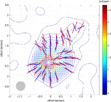
Figure 1: Left: Figure 1 from koch2012 showing the Submillimeter Array (SMA) 870 $\mu$m polarization map of the Collapsing core W51 e2 obtained by tang2009 . The thick red segments show the magnetic field orientation after rotation by 90^∘ of the polarization pseudo-vectors (see Introduction) where polarization was detected such that $p/\sigma_{p}>3$. The degree of polarization is not represented in this map. The blue pseudo-vectors show the gradient directions (see Section 3 and Section 4) of the dust emission continuum mapped at 1.3 mm by lai2001 with the Berkeley-Illinois-Maryland Association (BIMA). Right: Figure 2 from poidevin2013 showing the ADF of the SCUBA JCMT DR21 850 $\mu$m polarization maps (see Section 2).

2 Davis-Chandrasekhar and Fermi (DCF) method and Angular Dispersion function (ADF)

The DCF method was introduced in the middle of the twentieth century by davis1951 and cf1953 . It was first designed to get estimates of the POS magnetic field strength, $B_{pos}$, assuming a turbulent diffuse ISM. It was applied on polarimetry data obtained on star fields by hiltner1951 at visible wavelengths. In this regime, the polarization is produced by dichroic absorption of starlight by dust grain layers pervading the diffuse ISM, in a direction perpendicular to the one produced in emission at submm wavelengths by identical polarizing dust grains (see planck_ir_xxi ). Inferred from the data is a large-scale uniform magnetic field along the Galactic Plane (GP). The fluctuations around the mean of the distribution of the polarization pseudo-vectors are assumed by davis1951 and cf1953 to be produced by Alfvén waves that are coupled to the gas such that there is equipartition between kinetic and perturbed magnetic energies. With this model $B_{pos}$ is a function of the ISM gas density $\rho$, of the gas velocity dispersion $\sigma_{v}$, and of the polarization angle dispersion $\sigma_{\theta}$, such that: $B_{pos}=Q\sqrt{4\pi\rho}\frac{\sigma_{v}}{\sigma_{\theta}}$, where $Q$ is a factor of proportionality. With this method, cf1953 calculated a diffuse ISM $B_{pos}$ estimate of a few $\mu$G consistent with those obtained with other independent methods. Later on, in the 1990s, when polarimetry detectors at submm wavelengths started to be sensitive enough, the DCF method was used on submm maps of molecular clouds, meaning transposed to spatial scales 1000 to 10000 times smaller than the GP scale in regions of density two orders or more magnitudes that of the diffuse ISM density. The first comprehensive study was done by gonatas1990 from 10 measurements obtained at 100$\,\mu$m with the Kuiper Airborne Observatory (KAO) in the Orion Nebula, leading to $B_{pos}$ estimates of a few mG. The DCF method has been tested numerically by ostriker2001 and dfg2008 and some refinements to the calculations of $B_{pos}$ have been proposed. A review on the values of $Q$ has been given by poidevin2013 .

Improvements to the Method: Further major improvements to the method were designed by hildebrand2009 , houde2009 and houde2011 . The Angular Dispersion Function (ADF) was introduced by hildebrand2009 to avoid inaccurate estimates of magnetohydrodynamic or turbulent dispersion, as well as to avoid inaccurate estimates of $B_{pos}$, due to the large-scale, non turbulent field structure. The ADF is expressed by $<\Delta\Phi^{2}(l)>^{1/2}\equiv\left\{\frac{1}{N(l)}\Sigma_{i=1}^{N(l)}[\Phi(x)-\Phi(x+l)]^{2}\right\}^{1/2}$, where $\Phi(x)$ is the angle asssociated to the projected POS magnetic field vector $B(x)$ at position $x$ in a map. The difference in angle between two points is obtained by $\Delta\Phi(l)\equiv\Phi(x)-\Phi(x+l)$, and is calculated between the $N(l)$ pairs of vectors separated by displacement, or lag, $l$. $<...>$ denotes an average and $l=|l|$. The square of the ADF, a second order structure function, is also often used (e.g. dfg2008 ). One example of ADF is shown in Figure 1 (right panel), where the angular dispersion $b$ is the intercept of the fit at $l=0$. Correlations in polarization angles at lags $l$ smaller than the telescope beam ($1.22\lambda/D$) or than the turbulent correlation length ($\delta$) have to be avoided. The fit is ideally applied on the set of points calculated by taking into account the measurement uncertainties and such that the lag distance $l$ is smaller that the typical length scale $d$ for variations in the large-scale magnetic fields. Once $b$ is estimated from a map this method also provides an estimate of the turbulent to large-scale magnetic field strength ratio such that $\frac{<B_{t}^{2}>^{1/2}}{B_{pos}}=\frac{b}{\sqrt[]{2-b^{2}}}$, and the POS strength of the large-scale component is estimated by $B_{pos}\simeq\sqrt[]{8\pi\rho}\frac{\sigma_{v}}{b}$. The method to take into account the effect of the signal integration through the thickness of the clouds as well as across the area sustended by the telescope is fully incorporated by houde2009 . The authors also show how to evaluate the turbulent magnetic field correlation length scale from polarization maps obtained with sufficiently high resolution and high enough spatial sampling rate. Further examples are given and discussed by houde2011 as well as the application of the technique to interferometry measurements.

Results: The DCF method has been applied to data from many Galactic MCs obtained on sky patches, including Gould belt MCs (e.g. coude2019 ) and some of the closests low, intermediate or high star-forming regions. Estimates of $B_{pos}$ lie typically in the range of a few $\mu$G to a few mG. In OMC-1 the turbulent correlation length is estimated to $\delta\approx$ 10 mpc (e.g. houde2009 ). Independently of the uncertainties coming from the propagation of the errors, the estimates of $B_{pos}$ and $\delta$ will rely on the choice (or availabilty) of the gas tracers and of the value of $Q$ used for the calculation of $B_{pos}$ (e.g. see discussion in pattle2017 ). In principle accurate and reliable results can be obtained with polarization data of sufficient spatial resolution and high enough spatial sampling rate (houde2009 ). The DCF method has been applied to a large fraction of the sky by planck_ir_xix and on the full sky by planck2018_xii . Using the Planck Release 3 planck2018_xii have obtained the following relation between the ADF, $S$, and the fraction of polarization, $p$, as a function of the map resolution, $w$: $<S_{p}>=\frac{0^{\circ}.31}{p}\left(\frac{w}{160^{{}^{\prime}}}\right)$. The results are displayed in Figure 2 (top-left panel), and show that down to a resolution of $10^{\prime}$ the systematic decrease in $p$ with $N_{\rm H}$ is determined mostly by the magnetic-field structure. At a lower resolution of $2.5^{\prime}$, using the $500\mu$m BLASTPol polarization map of Vela C, fissel2016 discuss the dependence of $p$ on the dust temperature and on $N_{\rm H}$ and show that $p\varpropto N_{\rm H}^{-0.45}S^{-0.60}$, suggesting that dust grain alignment properties may also contribute to the decrease of $p$ in some conditions.

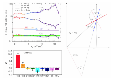
Figure 2: Top-Left: Figure 11 from planck2018_xii showing the $S\times p$ relation as a function of column density $N_{\rm H}$ where $w$ is the map resolution parameter (see Section 2). Bottom-Left: Figure 6 from fissel2019 showing the PRS $Z_{x}$ corrected for oversampling obtained with several molecular tracers (see Section 3). Right: Figure 3 from koch2012 showing the 90^∘ rotated P.A. $\alpha$, and the angle associated to the gradient orientation $\psi$, used to retrieve information on the magnetic field strength and significance (see Section 4).

3 Histogram of Relative Orientations (HROs) between ISM tracer structures and magnetic field structures

This method has been designed by soler2013 and subsequently applied to many molecular cloud regions (e.g. soler2017 , planck_ir_xxxv ). The concept of the method relies on the calculation of the gradient of the column density structure provided by a given material tracer (e.g. $N_{\rm H}$) in the pixels of a polarization map. As an illustration the blue pseudo-vectors displayed in Figure 1 (left panel), show the gradient orientations obtained from a dust emission continuum map. Once the gradients are quantified their relative orientation with the POS magnetic field orientations inferred from the P.A.s can be estimated and the HROs can be analysed. Several methods exist to calculate the gradients in a map as a function of the morphology structure of the object one is interested to isolate (see e.g. alina2019 and references therein). HROs can be built by considering the relative orientation of P.A.s with respect to the average orientation of a large-scale structure identified in a map (e.g. alina2019 ). More frequently, HROs are calculated by considering the relative orientation angle $\phi$ between the POS magnetic field $<\widehat{B}_{pos}>$ and a line tangent to the local iso-contour (see soler2013 , soler2017 , fissel2019 ) which is equivalent to the angle between the polarization direction $\widehat{E}$ and the intensity gradient $\bigtriangledown I$: $\phi=\rm arctan(|\bigtriangledown I\times\widehat{E}|,\bigtriangledown I.\widehat{E})$. Statistical measures of HROs have been quantified using the histogram shape parameter (e.g. soler2013 , soler2017 ), $\zeta=\frac{A_{0}-A_{90}}{A_{0}+A_{90}}$, where $A_{0}$ is a measure of the total number of points in the quartile $0^{\circ}<\phi<22^{\circ}.5$, and $A_{90}$ a measure of the same quantity in the quartile $67^{\circ}.5<\phi<90^{\circ}$. Smoother and more accurate definitions of $\zeta$ have been investigated by jow2018 . For this Rayleigh statistics $Z$ is used to test whether a given set ${\theta_{i}}$ of $n$ independent angles are uniformly distributed within the range$[0,2\pi]$. Using the relation $\theta=2\phi$, where $\phi$ is the relative orientation angle discussed above, jow2018 showed that the Projected Rayleigh Statistic (PRS) of $Z$: $Z_{x}=\Sigma_{i}^{n_{\rm ind}}\rm cos\theta{{}_{i}}/\sqrt{n_{\rm ind}/2}$, where $n_{\rm ind}$ is the number of independent data samples in the map, can be used to test for a preference for perpendicular or parallel alignment between the magnetic field orientations and the iso-contours. The variables $\zeta$ or $Z_{x}$ are often calculated on samples of data lying in different ranges of intensity of the material tracer map, and used to explore variations of the relative orientations between the magnetic field structures and the ISM morphology structures as a function of the column density or number density parameters. Figure 2 (bottom-left panel) shows the PRS obtained by fissel2019 using several molecular tracers. For each tracer, $Z_{x}>0(<0)$ indicates the $I$ structure preferentially aligns parallel (perpendicular) to $<\widehat{B}_{pos}>$.

Results: The main trend found from the analysis of HROs derived with lines tangent to local iso-contours is that the POS magnetic field orientations change from mostly parallel (or not clearly defined) to perpendicular with respect to the molecular cloud structures probed with a given material tracer (soler2017 , planck_ir_xxxv , fissel2019 ). This translates by a change of orientation from lower to higher column densities $N_{\rm H}$. In Vela C the transition is estimated to occur at molecular hydrogen number density of approximately $n_{\rm H}\approx 10^{3}\rm cm^{-3}$ (fissel2019 ). This local iso-contours approach has been tested by simulations (e.g. soler2013 ). In their study alina2019 first produce a component separation analysis of the magnetic fields in the diffuse ISM and in higher column density regions, and use image analysis technics to extract filaments and clumps embedded in different background column densities, i.e. showing density contrast varying with their environment. Their analysis of the HROs obtained between filaments, embedded clumps and internal and background magnetic field orientations lead to a more complex picture than in other studies. Overall their results support the possibility of magnetic fields strong enough to influence the formation of molecular clouds and also of their embedded clumps.

4 Polarization-Intensity Gradient Relation (P-IGR)

This method has been designed by koch2012 to study star-forming regions. In the case of negligible viscosity and infinite conductivity (ideal MHD case) the force equation is given by the following expression $\rho\left(\frac{\partial}{\partial t}+\mathbf{v}.\bigtriangledown\right)\mathbf{v}=-\bigtriangledown\left(P+\frac{B^{2}}{8\pi}\right)-\rho\bigtriangledown\phi+\frac{1}{4\pi}(\mathbf{B}.\bigtriangledown)\mathbf{B},$ where $\rho$ and v are the dust density and velocity, respectively. B is the magnetic field, $P$ is the hydrostatic dust pressure, $\phi$ is the gravitational potential resulting from the total mass contained in the region of interest and, $\bigtriangledown$ denotes the gradient. The left-hand side term in the equation represents the resulting motion of the dust produced by the right-hand side terms which are the gradients of the hydrostatic pressure terms of the gas, the magnetic field, and the gravitational potential together as well as the magnetic field tension term (last term). The force equation can be transformed and under several assumptions the magnetic field strength can in principle be derived geometrically at each position of a polarization map and expressed by: $B=\sqrt{\frac{\rm sin(\psi)}{\rm sin(\alpha)}(\bigtriangledown P+\rho\bigtriangledown\phi)4\pi R}$, where $\alpha$ = P.A.-90^∘, and $\psi$ is the angle associated to the gradient orientation. Figure 2 (right panel), illustrates the terms displayed in this equation. The red and blue pseudo-vectors displayed in the figure can be compared to those displayed in figure 1 (left panel) where the gradients in intensity are estimated assuming central symmetry towards the brightest pixel in the map, but the method can be generalized to arbitrary cloud shapes. An important outcome of the method is given by the magnetic field significance: $\Sigma_{B}\equiv\left(\frac{\rm sin(\psi)}{\rm sin(\alpha)}\right)_{local}=\left(\frac{F_{B}}{\mid F_{G}+F_{P}\mid}\right)_{local}$, which gives a direct physical meaning to the factor $\frac{\rm sin(\psi)}{\rm sin(\alpha)}$ derived geometrically from a map.

Results: The method provides a quantification of the local significance of the magnetic field force compared to the other forces in a model-independent way. In W51 e2 it allows derivations of the azimuthally averaged radial profile $B(r)\sim r^{-1/2}$ (koch2012 ). The potential of the method is explored in additional works (e.g. koch2018 and references therein). In their study, tang2019 propose that in G34 the varying relative importance between magnetic field, gravity, and turbulence from large-to-small-scale drives and explains the different fragmentation types seen at subparsec scales (no fragmentation, aligned fragmentation and clustered fragmentation).

5 Conclusions and perspectives

The methods discussed above are complementary to each other. If submm polarization maps are available at different resolutions they are suited to explore the role of magnetic fields, turbulence and gravity on different spatial scales. Their combination starts to give insights on the interplay between magnetic fields, gravity and turbulence (e.g. tang2019 ) and they are promising tools to shed light on the physics of hubs-filaments (e.g. andre2019 ) detected at subparsec scales in molecular clouds. In addition to these methods, getting estimates of the mean inclination with respect to the LOS of the large-scale ordered magnetic field considered as the main factor regulating the mean level of polarization in a map can help guiding the overall interpretation. In this regard, a method first proposed by poidevin2013 has been further explored by other authors (e.g. chen2019 ). Multi-wavelengths submm polarimetry of a region can give insights about polarization dust grain properties and also help to put constraints on the interpretation of the maps. On this matter we refer the reader to and2015 , vaillancourt2012 , shariff2019 and references therein.

Acknowledgments: FP acknowledges support from the Spanish Ministerio de Economia y Competitividad (MINECO) under grant numbers ESP2015-65597-C4-4-R and ESP2017-86852-C4-2-R.

References

- (1) J.F. Robitaille, and 3 coauthors, A&A 628, p.33-48 (2019).
- (2) F. Boulanger and 22 coauthors, JCAP, Issue 08, article id. 049 (2018).
- (3) B.G. Andersson, and 2 coauthors, ARA&A, vol. 53, p.501-539 (2015).
- (4) Y.-W. Tang, and 5 coauthors, ApJ 700, p.251-261 (2009)
- (5) P. M. Koch, and 2 coauthors, ApJ 747, p79-97 (2012)
- (6) S.-P. Lai, and 3 coauthors, 561, p.864-870 (2001)
- (7) L. Davis, 1951, Phys. Rev. 81, p.890-891
- (8) S. Chandrasekhar, and E. Fermi, ApJ, 118, p.113-115 (1953)
- (9) W. A. Hiltner, ApJ, 114, p.241-271 (1951)
- (10) Planck IR XIX, A&A 576, A106, 17pp (2015)
- (11) D. P. Gonatas, and 8 coauthors, ApJ 357, p.132-137 (1990)
- (12) E. C. Ostriker, and 2 coauthors, ApJ 546, p.980-1005 (2001)
- (13) D. Falceta-GonÃalves, and 2 coauthors, ApJ 679, p.537-551 (2008)
- (14) F. Poidevin, and 4 coauthors, ApJ 777, 112-126 pp. (2013)
- (15) R. H. Hildebrand, and 4 coauthors, ApJ 696, p.567-573 (2009)
- (16) M. Houde, and 4 coauthors, ApJ 706, p.1504-1516 (2009)
- (17) M. Houde, and 3 coauthors, ApJ 733, p.109-116 (2011)
- (18) S. Coudé, and 120 coauthors, Apj 877, p.88-104, 2019
- (19) K. Pattle, and 29 coauthors, ApJ 846, p.122-142 (2017)
- (20) Planck IR XIX, A&A 576, A104, 33pp (2015)
- (21) Planck 2018 Results XII, arXiv:1807.06212v2 (2019)
- (22) L. M. Fissel, and 29 coauthors, ApJ 824, p.134-154 (2016)
- (23) J. D. Soler, and 5 coauthors, ApJ 774, p.128-143 (2013)
- (24) J. D. Soler, and 30 coauthors, A&A 603, A64, 17pp.
- (25) Planck IR XXXV, A&A 586, p.138-166 (2016)
- (26) D. Alina, and 7 coauthors, MNRAS 485, p.2825-2843 (2019)
- (27) L. M. Fissel, and 39 coauthors, ApJ 878, p110-135 (2019).
- (28) D. L. Jow, and 7 coauthors, MNRAS 474, p.1018-1027 (2018)
- (29) P.M. Koch, and 5 coauthors, ApJ 855, p.39-57 (2018)
- (30) Y.-W. Tang, and 7 coauthors, ApJ 878, p.10-24 (2019)
- (31) Ph. André, and 4 coauthors, A&A, 629, L4, 8pp (2019)
- (32) J.E. Vaillancourt, and B.C. Matthews, ApJSS, 201, p.13-27 (2012)
- (33) J.A. Shariff, and 29 coauthors, ApJ 872, p.197-210 (2019)
- (34) C.-Y. Chen, and 4 coauthors, MNRAS 485, p.3499â3513 (2019)