Neural-network quantum states at finite temperature

Abstract

We propose a method to obtain the thermal-equilibrium density matrix of a many-body quantum system using artificial neural networks. The variational function of the many-body density matrix is represented by a convolutional neural network with two input channels. We first prepare an infinite-temperature state, and the temperature is lowered by imaginary-time evolution. We apply this method to the one-dimensional Bose-Hubbard model and compare the results with those obtained by exact diagonalization.

I Introduction

One of the challenging problems in physics is the determination of the properties of quantum many-body systems. Quantum many-body problems are difficult to solve, since the size of the Hilbert space exponentially increases with the size of the system. An approximate method to overcome this difficulty is the variational method, in which the huge Hilbert space is represented by a variational wave function with a tractable number of variational parameters. However, the variational method relies greatly on the physical insight of researchers to find sophisticated variational wave functions Feynman ; BCS .

Carleo and Troyer Carleo proposed the use of artificial neural networks to represent variational wave functions for quantum many-body states. It is known that artificial neural networks are very flexible and can approximate any function if the number of hidden units in the neural networks is sufficient. Using artificial neural networks as variational functions, therefore, we expect that quantum many-body wave functions can be approximated efficiently, in which the essential features of quantum many-body states are automatically captured as variational network parameters are optimized. This method has been applied to a variety of quantum many-body problems, and various properties of quantum many-body states represented by neural networks have been investigated Deng ; Chen ; Cai ; Gao ; SaitoL ; Nomura ; Kato ; Glasser ; Carleo08 ; Czischek ; Ruggeri ; Saito18 ; Levine ; ChooL ; Liang ; Luo ; Lu ; Choo .

Recently, artificial neural networks were also used to represent the density matrices of open quantum many-body systems Torlai ; Yoshioka ; Nagy ; Hartmann ; Vicentini . A density operator $\hat{\rho}$ contains more information than a pure state $|\psi\rangle$, and open quantum systems need more representation ability of neural networks than closed quantum systems. In Refs. Yoshioka ; Nagy ; Hartmann ; Vicentini , the master equations in the Lindblad form are solved using the variational Monte Carlo method, and the steady states of dissipative spin systems are obtained. The successful use of neural networks to represent density matrices opens up the application of machine learning not only to dissipative quantum systems, but also to finite-temperature states of quantum many-body systems.

Although the Boltzmann machine was used in the previous studies Torlai ; Yoshioka ; Nagy ; Hartmann ; Vicentini , in this paper, we use a convolutional neural network (CNN) textbook to represent the density matrix of a finite-temperature state. The CNN has been used to represent the ground states, i.e., pure states, of quantum many-body systems Kato ; Levine ; Liang ; Choo . In the case of the pure state $|\psi\rangle$, for the base $|\bm{n}\rangle$, the configuration of particles or spins $\bm{n}$ is input into the CNN, and the output of the CNN gives the amplitude $\langle\bm{n}|\psi\rangle$. For the density matrix, in the present study, we input $\bm{n}$ and $\bm{n}^{\prime}$ into the CNN with two input channels, and the output of the CNN gives the matrix element $\langle\bm{n}|\hat{\rho}|\bm{n}^{\prime}\rangle$ of the density operator $\hat{\rho}$. We first prepare the density matrix at infinite temperature with $\beta=(k_{B}T)^{-1}=0$, and the imaginary-time propagator $e^{-\Delta\beta\hat{H}}$ is applied to the density matrix successively to obtain $\hat{\rho}=e^{-\beta\hat{H}}$ at each $\beta$. A similar imaginary-time method was used to obtain the thermal equilibrium in matrix product states Verstraete ; Zwolak ; Feiguin . We apply our method to the Bose-Hubbard model, which describes cold bosonic atoms in optical lattices Jaksch . We calculate the finite-temperature density matrix of the Bose-Hubbard model in one-dimensional space and compare the results with those obtained by exact diagonalization. We also investigate the dependence of the accuracy of our method on various conditions, such as CNN structures.

This paper is organized as follows. Section II explains the method, Sec. III shows the numerical results, and Sec. IV provides the conclusions of the study.

II Method

To demonstrate the neural-network method for obtaining the finite-temperature density matrix, we apply it to the Bose-Hubbard model in one-dimensional space. The Hamiltonian is given by

$$\hat{H}=-\sum_{\langle i,j\rangle}{\hat{a}_{i}\hat{a}_{j}^{\dagger}}+\frac{U}{2}\sum_{i}\hat{n}_{i}(\hat{n}_{i}-1),$$ (1)

where $U$ is the on-site interaction energy, $\hat{a}_{i}$ is the annihilation operator of a boson at the $i$th site, $\hat{n}_{i}=\hat{a}_{i}^{\dagger}\hat{a}_{i}$ is the number operator, and $\langle i,j\rangle$ represents adjacent sites. The energy is normalized in such a way that the hopping coefficient becomes unity. Such a system can be realized by ultracold bosonic atoms loaded in an optical lattice Jaksch . We assume the periodic boundary condition, $\hat{a}_{M+1}=\hat{a}_{1}$, where $M$ is the number of sites. A pure quantum state can be expanded by the Fock-state bases $|\bm{n}\rangle$, where $\bm{n}=(n_{1},n_{2},\cdots,n_{M})$ represents the number of bosons in each site. We consider a canonical ensemble at temperature $T=(k_{B}\beta)^{-1}$ with total number of bosons $N$. The number of Fock-state bases $|\bm{n}\rangle$ satisfying $\sum_{i}n_{i}=N$ is $N_{\rm base}=(N+M-1)!/[N!(M-1)!]$, which increases exponentially with $N$ and $M$. We restrict ourselves to the case of $N=M$ in the following analysis. In this case, at zero temperature, the system becomes a Mott insulator for large $U$, and the system exhibits superfluidity for small $U$. At finite temperature, the normal phase emerges Dicker around the Mott insulator and superfluid regions in the phase diagram. Since all the matrix elements $\langle\bm{n}|e^{-\epsilon\hat{H}}|\bm{n}^{\prime}\rangle$ for infinitesimal $\epsilon>0$ can be taken to be real and nonnegative without loss of generality, all the matrix elements of the thermal density matrix $\langle\bm{n}|e^{-\beta\hat{H}}|\bm{n}^{\prime}\rangle$, which are decomposed to matrix products of $\langle\bm{n}|e^{-\epsilon\hat{H}}|\bm{n}^{\prime}\rangle$, can be taken to be real and nonnegative.

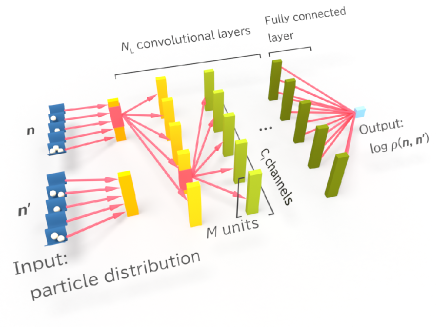
Figure 1: (color online) Schematic illustration of the CNN to represent the density matrix $\rho(\bm{n},\bm{n}^{\prime})=\langle\bm{n}|\hat{\rho}|\bm{n}^{\prime}\rangle$. The one-dimensional configurations of bosons $\bm{n}$ and $\bm{n}^{\prime}$ on $M$ sites are input into the two input channels. Successive $N_{L}$ convolutional layers are followed by a fully-connected layer, which gives output $u^{\rm(out)}$. The matrix element of the density matrix $\rho(\bm{n},\bm{n}^{\prime})$ is given by $e^{u^{\rm(out)}}$.

We employ the CNN textbook to represent the density matrix $\langle\bm{n}|\hat{\rho}|\bm{n}^{\prime}\rangle\equiv\rho(\bm{n},\bm{n}^{\prime})$ of the system (see Fig. 1). The inputs into the CNN are $\bm{n}$ and $\bm{n}^{\prime}$, which we denote as $\bm{u}^{(0)}_{1}$ and $\bm{u}^{(0)}_{2}$, respectively, i.e., the CNN has two input channels, with each of size $M$. The first hidden layer is calculated as

$$u_{m,j}^{(1)}=\sum_{k=1}^{2}\sum_{p=0}^{F_{1}-1}W_{k,m,p}^{(1)}u_{k,j+p}^{(0)}+b_{m}^{(1)},$$ (2)

and these are propagated to the deeper layers as

$$u_{m,j}^{(l)}=\sum_{k=1}^{C_{l-1}}\sum_{p=0}^{F_{l}-1}W_{k,m,p}^{(l)}f(u_{k,j+p}^{(l-1)})+b_{m}^{(l)},$$ (3)

where $\bm{W}_{k,m}^{(l)}$ is the one-dimensional filter with size $F_{l}$, $\bm{b}^{(l)}$ is the bias, and $C_{l}$ is the number of channels in the $l$th hidden layer. In Eqs. (2) and (3), the subscripts $m$ and $k$ identify the channels. The number of units in each channel in the input and hidden layers is $M$, i.e., $\bm{u}_{m}^{(l)}=(u_{m,1}^{(l)},u_{m,2}^{(l)},\cdots,u_{m,M}^{(l)})$, which satisfies the periodic boundary condition, $u_{m,M+1}^{(l)}=u_{m,1}^{(l)}$. We adopt the leaky ReLU textbook function as the activation function $f$,

$$f(x)=\begin{cases}x&(x\geq 0)\\ ax&(x<0)\end{cases}$$ (4)

with a constant $a>0$. After $N_{L}$ convolutional layers, the CNN finally gives a single output value $u^{\rm(out)}$ through the fully-connected layer as

$$u^{\rm(out)}=\sum_{m=1}^{C_{L}}\sum_{j=1}^{M}W^{\rm(fc)}_{m,j}u_{m,j}^{(L)}.$$ (5)

The network parameters are thus the filters $\bm{W}_{k,m}^{(l)}$ and biases $\bm{b}^{(l)}$ in the convolutional layers, and weights $\bm{W}_{m}^{\rm(fc)}$ in the fully-connected layer, which are all taken to be real, and therefore the output $u^{\rm(out)}$ is real. In the following, we abbreviate these network parameters as $\bm{W}$. Using the output $u^{\rm(out)}$ in Eq. (5), the matrix element of the density matrix is represented as

$$\rho(\bm{n},\bm{n}^{\prime})=e^{u^{\rm(out)}}.$$ (6)

Although such representation of the density matrix using the CNN does not assure its Hermiticity and positive definiteness, unlike the Boltzmann-machine representation proposed in Ref. Torlai , we will see that the Hermiticity and positive definiteness are approximately satisfied during the imaginary-time evolution.

The imaginary-time evolution of the density matrix is realized as follows. Suppose that we have a CNN that represents the density matrix at inverse temperature $\beta$, $\rho_{\beta}(\bm{n},\bm{n}^{\prime})=\langle\bm{n}|e^{-\beta\hat{H}}|\bm{n}^{\prime}\rangle$. The value of a matrix element of the density matrix at $\beta+\Delta\beta$ is calculated from $\rho_{\beta}(\bm{n},\bm{n}^{\prime})$ as

$$\rho_{\beta+\Delta\beta}(\bm{n},\bm{n}^{\prime})=\langle\bm{n}|e^{-(\beta+\Delta\beta)\hat{H}}|\bm{n}^{\prime}\rangle$$ (7)

$$= \sum_{\bm{n}_{1},\bm{n}_{2}}\langle\bm{n}|e^{-\frac{\Delta\beta\hat{H}}{2}}|\bm{n}_{1}\rangle\rho_{\beta}(\bm{n}_{1},\bm{n}_{2})\langle\bm{n}_{2}|e^{-\frac{\Delta\beta\hat{H}}{2}}|\bm{n}^{\prime}\rangle$$

$$= \rho_{\beta}(\bm{n},\bm{n}^{\prime})-\frac{\Delta\beta}{2}\sum_{\bm{n}_{1}}\Bigl{[}\langle\bm{n}|\hat{H}|\bm{n}_{1}\rangle\rho_{\beta}(\bm{n}_{1},\bm{n}^{\prime})$$

$$+\rho_{\beta}(\bm{n},\bm{n}_{1})\langle\bm{n}_{1}|\hat{H}|\bm{n}^{\prime}\rangle\Bigr{]}+\cdots+O(\Delta\beta^{K+1}),$$

where we expand $e^{-\Delta\beta\hat{H}/2}$ with respect to $\Delta\beta$ in the last line. We cut off the $O(\Delta\beta^{K+1})$ terms in Eq. (7). By this approximation, the number of terms in the last line of Eq. (7) is reduced to $O(M^{K})$, since the number of nonzero matrix elements $\langle\bm{n}|\hat{H}^{K}|\bm{n}^{\prime}\rangle$ is $O(M^{K})$. We can thus calculate any matrix elements $\rho_{\beta+\Delta\beta}(\bm{n},\bm{n}^{\prime})$ at the inverse temperature $\beta+\Delta\beta$, when we have the CNN that represents the density matrix at $\beta$. We next need to construct a CNN that represents the density matrix $\rho_{\beta+\Delta\beta}(\bm{n},\bm{n}^{\prime})$.

In general, we can optimize a CNN so as to represent a desired density matrix $\rho_{\rm target}(\bm{n},\bm{n}^{\prime})$ by minimizing

$$L=\frac{1}{2}\sum_{\bm{n},\bm{n}^{\prime}}\left[\rho(\bm{n},\bm{n}^{\prime})-\rho_{\rm target}(\bm{n},\bm{n}^{\prime})\right]^{2},$$ (8)

where $\rho(\bm{n},\bm{n}^{\prime})$ is the density matrix represented by the CNN to be optimized. We denote the network parameters of this CNN as $\bm{W}$. We can update $\bm{W}$ to reduce the value of $L$ using its gradient with respect to $\bm{W}$ as

$$\frac{\partial L}{\partial w}=\sum_{\bm{n},\bm{n}^{\prime}}\frac{\partial\rho(\bm{n},\bm{n}^{\prime})}{\partial w}\left[\rho(\bm{n},\bm{n}^{\prime})-\rho_{\rm target}(\bm{n},\bm{n}^{\prime})\right],$$ (9)

where $w$ is one of the network parameters $\bm{W}$. Here, instead of Eq. (9), we introduce a modified gradient as

$$\sum_{\bm{n},\bm{n}^{\prime}}P(\bm{n},\bm{n}^{\prime})\frac{\partial\rho(\bm{n},\bm{n}^{\prime})}{\partial w}\left[\rho(\bm{n},\bm{n}^{\prime})-\rho_{\rm target}(\bm{n},\bm{n}^{\prime})\right],$$ (10)

where

$$P(\bm{n},\bm{n}^{\prime})=\frac{\left[\rho(\bm{n},\bm{n}^{\prime})-\rho_{\rm target}(\bm{n},\bm{n}^{\prime})\right]^{2}}{\sum_{\bm{n},\bm{n}^{\prime}}\left[\rho(\bm{n},\bm{n}^{\prime})-\rho_{\rm target}(\bm{n},\bm{n}^{\prime})\right]^{2}}.$$ (11)

Since the factor $P(\bm{n},\bm{n}^{\prime})$ emphasizes the terms with larger deviation $\left|\rho(\bm{n},\bm{n}^{\prime})-\rho_{\rm target}(\bm{n},\bm{n}^{\prime})\right|$, we expect more efficient convergence of $\rho(\bm{n},\bm{n}^{\prime})$ to $\rho_{\rm target}(\bm{n},\bm{n}^{\prime})$ using Eq. (10) than Eq. (9). The form of Eq. (10) is also suitable for Metropolis sampling. Since the summation $\sum_{\bm{n},\bm{n}^{\prime}}$ cannot be taken exactly for a large system, we calculate the summation by the Monte Carlo method with Metropolis sampling of $\bm{n}$ and $\bm{n}^{\prime}$ with probability distribution $P(\bm{n},\bm{n}^{\prime})$. Using the gradient in Eq. (10), the network parameters are updated using the Adam scheme textbook ; Kingma , until $\rho(\bm{n},\bm{n}^{\prime})$ converges sufficiently.

We thus generate the thermal density matrix as follows. We first prepare the initial CNN that represents the density matrix at infinite temperature $\beta=0$, which is used as the initial density matrix of the imaginary-time evolution. Such a CNN can be constructed by the method described above with $\rho_{\rm target}(\bm{n},\bm{n}^{\prime})=\lim_{\beta\rightarrow 0}\langle\bm{n}|e^{-\beta\hat{H}}|\bm{n}^{\prime}\rangle=\delta_{\bm{n},\bm{n}^{\prime}}$, starting from random network parameters. Next, we set the target as $\rho_{\rm target}(\bm{n},\bm{n}^{\prime})=\rho_{\Delta\beta}(\bm{n},\bm{n}^{\prime})$, which can be calculated using Eq. (7). We prepare another CNN and optimize it to represent this target, which yields the CNN that represents $\rho_{\Delta\beta}(\bm{n},\bm{n}^{\prime})$. Repeating this procedure, we obtain CNNs that represent $\rho_{2\Delta\beta}$, $\rho_{3\Delta\beta}$, $\cdots$, successively. In each step of the imaginary-time evolution, the initial values of the network parameters for $\rho_{n\Delta\beta}$ are set to those for $\rho_{(n-1)\Delta\beta}$ to facilitate convergence.

The expectation value of an observable $\hat{A}$ is written as

$$\langle\hat{A}\rangle = \frac{\mathrm{Tr}(\hat{\rho}\hat{A})}{\mathrm{Tr}\hat{\rho}}=\frac{\sum_{\bm{n},\bm{n}^{\prime}}\rho(\bm{n},\bm{n}^{\prime})\langle\bm{n}^{\prime}|\hat{A}|\bm{n}\rangle}{\sum_{\bm{n}}\rho(\bm{n},\bm{n})}$$ (12)

$$= \sum_{\bm{n}}P(\bm{n})A(\bm{n}),$$

where $\mathrm{Tr}$ indicates trace, $P(\bm{n})=\rho(\bm{n},\bm{n})/\sum_{\bm{n}}\rho(\bm{n},\bm{n})$ and $A(\bm{n})=\sum_{\bm{n}^{\prime}}\rho(\bm{n},\bm{n}^{\prime})\langle\bm{n}^{\prime}|\hat{A}|\bm{n}\rangle/\rho(\bm{n},\bm{n})$. The summation in the second line of Eq. (12) is calculated by the Monte Carlo method with Metropolis sampling of $\bm{n}$ with probability distribution $P(\bm{n})$.

III Results

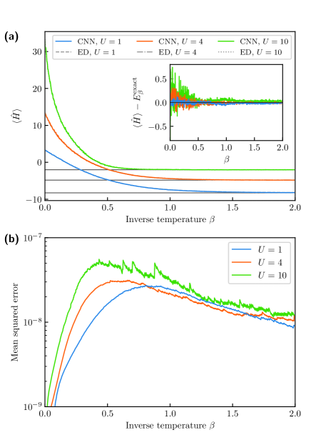
Figure 2: (color online) Imaginary-time evolution of the density matrix represented by a CNN for $U=1$, 4, and 10. (a) Expectation value of the Hamiltonian $\langle\hat{H}\rangle$. The lines of the energies $E_{\beta}^{\rm exact}$ obtained by exact diagonalization (ED) are also drawn, which however almost overlap with the lines obtained by our method and cannot be seen. The horizontal lines represent the exact energies of the ground states. The inset shows the error in the energy $\langle\hat{H}\rangle-E_{\beta}^{\rm exact}$. (b) Mean-squared error $\delta\rho$ defined in Eq. (13).

We consider a system of $M=5$ sites with $N=5$ particles. The CNN consists of $N_{L}=4$ convolutional layers with filter size $F_{1}=F_{2}=F_{3}=F_{4}=5$ and $C_{1}=C_{2}=C_{3}=C_{4}=16$ channels. The constant in the leaky ReLU in Eq. (4) is taken to be $a=0.3$. The imaginary-time evolution is generated with $\Delta\beta\sim 10^{-3}$, where we take the terms up to the second order of $\Delta\beta$ in the expansion in Eq. (7) (i.e., $K=2$). We take 2000 samples in the Metropolis sampling to calculate the gradient in Eq. (10) in each Adam optimization step. The optimization steps are performed 2000 times to obtain the next density matrix $\rho_{\beta+\Delta\beta}$ from $\rho_{\beta}$ in the imaginary-time evolution. In order to avoid exponential growth or decay of $\langle\bm{n}|e^{-\beta\hat{H}}|\bm{n}^{\prime}\rangle$ in the imaginary-time evolution, we add an appropriate constant to the Hamiltonian in each step.

Figure 2(a) shows the imaginary-time evolution of the expectation value of the energy $\langle\hat{H}\rangle$ obtained by our method for $U=1$, $4$, and $10$. In Fig. 2(a), we also plot the exact energy $E_{\beta}^{\rm exact}$ obtained by the exact diagonalization of the Hamiltonian. The lines of $\langle\hat{H}\rangle$ almost overlap with those of $E_{\beta}^{\rm exact}$. The error in the energy is $|\langle\hat{H}\rangle-E_{\beta}^{\rm exact}|\sim 0.1$. In Fig. 2(b), we plot the mean-squared error in the matrix elements of the density matrix, defined as Hartmann

$$\delta\rho=\frac{1}{N_{\rm base}^{2}}\sum_{\bm{n},\bm{n}^{\prime}}\left[\rho_{\beta}(\bm{n},\bm{n}^{\prime})-\rho_{\beta}^{\rm exact}(\bm{n},\bm{n}^{\prime})\right]^{2},$$ (13)

where $\rho_{\beta}^{\rm exact}(\bm{n},\bm{n}^{\prime})$ is the density matrix obtained by exact diagonalization of the Hamiltonian, and the summation is taken over all $\bm{n}$ and $\bm{n}^{\prime}$. In calculating $\delta\rho$, the density matrix is normalized as $\sum_{\bm{n}}\rho_{\beta}(\bm{n},\bm{n})=1$. The error $\delta\rho$ in Fig. 2(b) is less than $10^{-7}$. Thus, our method works well for whole temperature region and both for superfluid and Mott insulator regimes.

In Fig. 2(b), $\delta\rho$ increases for the early stage of the imaginary-time evolution ($\beta\lesssim 0.5$), and then $\delta\rho$ decreases with $\beta$. This is because the imaginary-time evolution $e^{-\Delta\beta\hat{H}/2}\hat{\rho}e^{-\Delta\beta\hat{H}/2}$ eliminates excited states in $\hat{\rho}$, and then also eliminates errors arising during the imaginary-time evolution. For $\beta\rightarrow\infty$, the density matrix converges to the ground state, even if errors arise during the imaginary-time evolution.

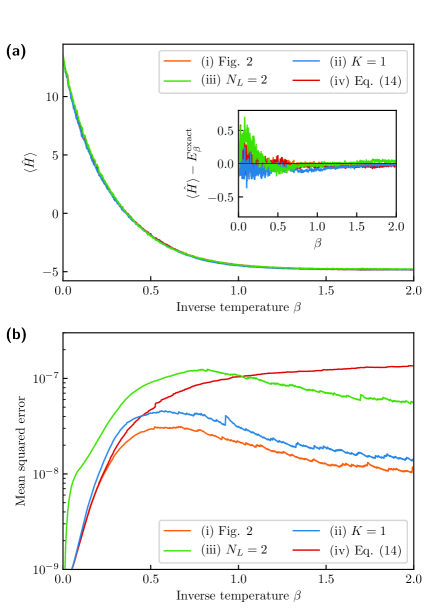
Figure 3: (color online) Dependence of the accuracy on various conditions for $U=4$, where (i) the same as in Fig. 2, (ii) the cutoff order in Eq. (7) is reduced to $K=1$, (iii) the number of convolutional layers is reduced to $N_{L}=2$, and (iv) the asymmetric expansion in Eq. (LABEL:dbeta2) is used with $K=2$. (a) Expectation value of the Hamiltonian $\langle\hat{H}\rangle$. The inset shows the error in the energy $\langle\hat{H}\rangle-E_{\beta}^{\rm exact}$. (b) Mean-squared error $\delta\rho$ defined in Eq. (13).

The errors arise from various sources: the cutoff in the expansion in Eq. (7), the representation ability of the CNN, the statistical errors due to the Monte Carlo sampling, and insufficient convergence in the Adam optimization. Figure 3 shows the dependence of the results on various conditions. We see that the errors are increased by reducing the cutoff order in Eq. (7) from $K=2$ to $K=1$ [the line (ii) in Fig. 3] or reducing the number of convolutional layers from $N_{L}=4$ to $N_{L}=2$ [the line (iii)]. We also confirmed that the accuracy is lowered by reducing the number of samples in the Metropolis sampling or the number of iterations in the Adam optimization (data not shown). In Fig. 3, we also examine a different form of expansion of $e^{-\Delta\beta\hat{H}}$ instead of the symmetric expansion in Eq. (7):

$$\rho_{\beta+\Delta\beta}(\bm{n},\bm{n}^{\prime}) = \langle\bm{n}|e^{-(\beta+\Delta\beta)\hat{H}}|\bm{n}^{\prime}\rangle$$

$$= \sum_{\bm{n}^{\prime\prime}}\langle\bm{n}|e^{-\Delta\beta\hat{H}}|\bm{n}^{\prime\prime}\rangle\langle\bm{n}^{\prime\prime}|e^{-\beta\hat{H}}|\bm{n}^{\prime}\rangle$$

$$\simeq \sum_{k=1}^{K}\frac{(-\Delta\beta)^{k}}{k!}\sum_{\bm{n}^{\prime\prime}}\langle\bm{n}|\hat{H}^{k}|\bm{n}^{\prime\prime}\rangle\rho_{\beta}(\bm{n}^{\prime\prime},\bm{n}^{\prime}),$$

where the propagator $e^{-\Delta\beta\hat{H}}$ always operates from the left-hand side of $\rho_{\beta}$. The line (iv) in Fig. 3 shows the result using this asymmetric expansion with $K=2$. The mean-squared error $\delta\rho$ monotonically increases for Eq. (LABEL:dbeta2). This is because the operator $e^{-\Delta\beta\hat{H}}$ in the asymmetric form in Eq. (LABEL:dbeta2) only eliminates excited states in the ket vectors in the density operator, and therefore, once errors arise in the bra vectors during the imaginary-time evolution, the errors remain for $\beta\rightarrow\infty$.

IV Conclusions

We proposed a method to represent a many-body density matrix using a convolutional neural network (CNN), where the particle configurations $\bm{n}$ and $\bm{n}^{\prime}$ are input into the CNN to produce the value of $\langle\bm{n}|\hat{\rho}|\bm{n}^{\prime}\rangle$. We also proposed a method to obtain the density matrix at finite temperature through the imaginary-time evolution of the density matrix represented by the CNN. We applied our method to the one-dimensional Bose-Hubbard model, and demonstrated the imaginary-time evolution, which showed that the finite-temperature density matrix obtained by our method agrees well with that obtained by exact diagonalization of the Hamiltonian. We have also investigated the dependence of the accuracy on different conditions.

Neural network quantum states are also efficient for representing many-body states of fermions Nomura , and therefore we expect that our method can also be applied to systems with negative-sign problems, which will be complementary to the quantum Monte Carlo method to investigate finite-temperature properties. The present method can also be extended to higher spatial dimensions in a straightforward manner.

- (1) R. P. Feynman, Application of quantum mechanics to liquid helium, Prog. Low Temp. Phys. 1, 17 (1955).
- (2) J. Bardeen, L. N. Cooper, and J. R. Schrieffer, Theory of superconductivity, Phys. Rev. 108, 1175 (1957).
- (3) G. Carleo and M. Troyer, Solving the quantum many-body problem with artificial neural networks, Science 355, 602 (2017).
- (4) D.-L. Deng, X. Li, and S. Das Sarma, Quantum entanglement in neural network states, Phys. Rev. X 7, 021021 (2017).
- (5) J. Chen, S. Cheng, H. Xie, L. Wang, and T. Xiang, Equivalence of restricted Boltzmann machines and tensor network states, Phys. Rev. B 97, 085104 (2018).
- (6) Z. Cai and J. Liu, Approximating quantum many-body wave-functions using artificial neural networks, Phys. Rev. B 97, 035116 (2018).
- (7) X. Gao and L.-M. Duan, Efficient representation of quantum many-body states with deep neural networks, Nat. Commun. 8, 662 (2017).
- (8) H. Saito, Solving the Bose-Hubbard Model with machine learning, J. Phys. Soc. Jpn. 86, 093001 (2017).
- (9) Y. Nomura, A. S. Darmawan, Y. Yamaji, and M. Imada, Restricted Boltzmann machine learning for solving strongly correlated quantum systems, Phys. Rev. B 96, 205152 (2017).
- (10) H. Saito and M. Kato, Machine learning technique to find quantum many-body ground states of bosons on a lattice, J. Phys. Soc. Jpn. 87, 014001 (2018).
- (11) I. Glasser, N. Pancotti, M. August, I. D. Rodriguez, and J. I. Cirac, Neural-network quantum states, string-bond states, and chiral topological states, Phys. Rev. X 8, 011006 (2018).
- (12) M. Ruggeri, S. Moroni, and M. Holzmann, Nonlinear network description for many-body quantum systems in continuous space, Phys. Rev. Lett. 120, 205302 (2018).
- (13) G. Carleo, Y. Nomura, and M. Imada, Constructing exact representations of quantum many-body systems with deep neural networks, Nat. Commun. 9, 5322 (2018).
- (14) S. Czischek, M. Gärttner, and T Gasenzer, Quenches near Ising quantum criticality as a challenge for artificial neural networks, Phys. Rev. B 98, 024311 (2018).
- (15) H. Saito, Method to solve quantum few-body problems with artificial neural networks, J. Phys. Soc. Jpn. 87, 074002 (2018).
- (16) Y. Levine, O. Sharir, N. Cohen, and A. Shashua, Quantum entanglement in deep learning architectures, Phys. Rev. Lett. 122, 065301 (2019).
- (17) K. Choo, G. Carleo, N. Regnault, and T. Neupert, Symmetries and many-body excitations with neural-network quantum states, Phys. Rev. Lett. 121, 167204 (2018).
- (18) X. Liang, W.-Y. Liu, P.-Z. Lin, G.-C. Guo, Y.-S. Zhang, and L. He, Solving frustrated quantum many-particle models with convolutional neural networks, Phys. Rev. B 98, 104426 (2018).
- (19) D. Luo and B. K. Clark, Backflow transformations via neural networks for quantum many-body wave functions, Phys. Rev. Lett. 122, 226401 (2019).
- (20) S. Lu, X. Gao, and L.-M. Duan, Efficient representation of topologically ordered states with restricted Boltzmann machines, Phys. Rev. B 99, 155136 (2019).
- (21) K. Choo, T. Neupert, and G. Carleo, Two-dimensional frustrated - model studied with neural network quantum states, Phys. Rev. B 100, 125124 (2019).
- (22) G. Torlai and R. G. Melko, Latent space purification via neural density operators, Phys. Rev. Lett. 120, 240503 (2018).
- (23) N. Yoshioka and R. Hamazaki, Constructing neural stationary states for open quantum many-body systems, Phys. Rev. B 99, 214306 (2019).
- (24) A. Nagy and V. Savona, Variational quantum Monte Carlo method with a neural-network ansatz for open quantum systems, Phys. Rev. Lett. 122, 250501 (2019).
- (25) M. J. Hartmann and G. Carleo, Neural-network approach to dissipative quantum many-body dynamics, Phys. Rev. Lett. 122, 250502 (2019).
- (26) F. Vicentini, A. Biella, N. Regnault, and C. Ciuti, Variational neural-network ansatz for steady states in open quantum systems, Phys. Rev. Lett. 122, 250503 (2019).
- (27) For example, I. Goodfellow, Y. Bengio, and A. Courville, Deep learning (MIT Press, Massachusetts, 2016)
- (28) F. Verstraete, J. J. García-Ripoll, and J. I. Cirac, Matrix product density operators: Simulation of finite-temperature and dissipative systems, Phys. Rev. Lett. 93, 207204 (2004).
- (29) M. Zwolak and G. Vidal, Mixed-state dynamics in one-dimensional quantum lattice systems: A time-dependent superoperator renormalization algorithm, Phys. Rev. Lett. 93, 207205 (2004).
- (30) A. E. Feiguin and S. R. White, Finite-temperature density matrix renormalization using an enlarged Hilbert space, Phys. Rev. B 72, 220401(R) (2005).
- (31) D. Jaksch, C. Bruder, J. I. Cirac, C. W. Gardiner, and P. Zoller, Cold bosonic atoms in optical lattices, Phys. Rev. Lett. 81, 3108 (1998).
- (32) D. B. M. Dickerscheid, D. van Oosten, P. J. H. Denteneer, and H. T. C. Stoof, Ultracold atoms in optical lattices, Phys. Rev. B 68, 043623 (2003).
- (33) D. P. Kingma and J. L. Ba, Adam: A method for stochastic optimization, arXiv:1412.6980.