The use of Kepler solver in numerical integrations of quasi-Keplerian orbits

Abstract

A Kepler solver is an analytical method used to solve a two-body problem. In this paper, we propose a new correction method by slightly modifying the Kepler solver. The only change to the analytical solutions is that the obtainment of the eccentric anomaly relies on the true anomaly that is associated to a unit radial vector calculated by an integrator. This scheme rigorously conserves all integrals and orbital elements except the mean longitude. However, the Kepler energy, angular momentum vector and Laplace-Runge-Lenz vector for perturbed Kepler problems are slowly-varying quantities. However, their integral invariant relations give the quantities high-precision values that directly govern five slowly-varying orbital elements. These elements combined with the eccentric anomaly determine the desired numerical solutions. The newly proposed method can considerably reduce various errors for a post-Newtonian two-body problem compared with an uncorrected integrator, making it suitable for a dissipative two-body problem. Spurious secular changes of some elements or quasi-integrals in the outer solar system may be caused by short integration times of the fourth-order Runge-Kutta algorithm. However, they can be eliminated in a long integration time of $10^{8}$ years by the proposed method, similar to Wisdom-Holman second-order symplectic integrator. The proposed method has an advantage over the symplectic algorithm in the accuracy but gives a larger slope to the phase error growth.

1 introduction

In a relative coordinate system, a pure two-body problem in the solar system is a system with three degrees of freedom. In this system, the Kepler energy, relative angular momentum vector and Laplace-Runge-Lenz (LRL) vector are seven integrals of motion. However, only five of them are independent due to the seven quantities satisfying two relations (hereafter, the so-called seven integrals in the pure two-body problem include dependent and independent integrals). They correspond to five constant orbital elements. In this case, the problem is integrable and has an analytical solution.

Regardless of whether $N$-body gravitational problems with $N>2$ perform quasi-Keplerian motions (i.e. the Keplerian motions with small perturbations; orbits for the quasi-Keplerian motions are quasi-Keplerian orbits), they are consistently non-integrable and have no analytical solutions. Numerical integration methods are convenient tools to solve them. Geometric integrators (Hairer et al. 1999) can preserve one or more physical/geometric properties of these systems. The properties contain structures, integrals, symmetries, reversing symmetries and phase-space volumes. Symplectic integrators (Ruth 1983; Feng 1985; Wisdom $\&$ Holman 1991; Zhong et al. 2010; Mei et al. 2013a, 2013b) are a class of geometric integration methods that conserve symplectic structures and phase-space volumes of Hamiltonian systems and have no secular drift in energy errors. They are particularly suitable for studying the qualitative properties on the long-term evolution of Hamiltonian systems because of these advantages. Symmetrical methods (Quinlan $\&$ Tremaine 1990), extended phase space methods (Pihajoki 2015; Liu et al. 2016; Luo et al. 2017; Li $\&$ Wu 2017) and energy-conserving schemes (Chorin et al. 1978; Feng 1985; Bacchini et al. 2018a, 2018b; Hu et al. 2019) belong to the geometric integrators. Although non-geometric integrators, such as Runge-Kutta methods, do not satisfy such geometric properties, they have wider applications than the geometric integrators. In addition, they provide more accurate numerical solutions than the same order geometric integrators (excluded those from the non-geometric integrators reformed) in a short integration time. In this case, their numerical results should be reliable.

However, the non-geometric integrators can be reformed as the geometric ones by means of some particular treatments. One method includes one or more integrals in a set of differential equations, thereby enabling the orbits change from the Lyapunov’s instability to the Lyapunov’s stability. Thus, the numerical solutions are consistently confined to the integral surface in the phase space and the fast growth of various numerical errors can typically be suppressed. This technique is the stabilizing method of Baumgarte (1972, 1973). Its applications are given in (Ascher et al. 1995; Chin 1995; Avdyushev 2003). Another stabilization path is the manifold correction scheme of Nacozy (1971), where stabilizing terms are directly added to the numerical solutions. This approach applies Lagrange multipliers to take the integrated orbits back to the original integral hypersurface along the least-squares shortest path. In this way, the corrected error of an integral is the square of the uncorrected one. This condition indicates that the correction solutions do not rigorously satisfy the integral. Following this basic idea, several authors focused on the application and effectiveness of manifold correction methods (Murison 1989; Chin 1995; Zhang 1996; Wu et al. 2006). The steepest descending method for the approximate consistency of the Kepler energy of the two-body problem suppresses the fast growth of integration errors in the semimajor axis (Wu et al. 2007). The approximate conservation of the seven integrals results in the five constant elements in the two-body problem (Ma et al. 2008a). In addition to these manifold correction methods that approximately satisfy the integrals, methods that rigorously satisfy the integrals have been developed. For example, the scaling method of Fukushima (2003a) and the velocity scaling method of Ma et al. (2008b) can exactly conserve the energy (associated to the semimajor axis) of the two-body problem. The dual scaling method for the rigorous consistency of the Kepler energy and LRL vector in the two-body problem is effective to control the growth of integration errors in the semimajor axis, eccentricity and longitude of pericenter (Fukushima 2003b). The rotation method for rigorously satisfying the angular momentum vector of the two-body problem reduces the growth of integration errors in the inclination and longitude of the ascending node (Fukushima 2003c). The linear transformation method of Fukushima (2004) is the best among Fukushima’s manifold correction methods because it simultaneously and rigorously satisfies the Kepler energy, angular momentum vector and LRL vector in the two-body problem. It can intensively reduce the integration errors in various orbital elements at small additional computational cost.

Seven integrals of motion, including the total energy, total momentum vector and total angular momentum vector, are consistently present for the quasi-Keplerian motions in a five-body system of the Sun and four outer planets. Unfortunately, the constancy of the total energy and total angular momentum does not exhibit good performance (Hairer et al. 1999). Individual Kepler energies, angular momentum vectors and LRL vectors must be corrected. However, these quantities are not constant and should slowly vary in this case. They are called slowly-varying quantities. No integrals of motion are available in dissipative and other nonconservative systems. The above correction methods become useless in these cases. These slowly-varying individual quantities obtained from their integral invariant relations (Szebehely $\&$ Bettis 1971; Huang $\&$ Innanen 1983) have higher accuracies than those directly determined by the integrated positions and velocities and can be taken as reference values of correcting the errors. In this way, the above correction methods (e.g. Fukushima 2003a, 2003b, 2003c, 2004; Wu et al. 2007; Ma et al. 2008a, 2008b) remain valid. These correction methods are not limited to treating conservative quasi-Keplerian problems. Wang et al. (2016, 2018) confirmed that the velocity scaling method of Ma et al. (2008b) combined with the integral invariant relation is effective in enhancing the quality of numerical integrations of non-Keplerian motions of nonconservative elliptic restricted three-body problems and dissipative circular restricted three-body problems.

A perturbed two-body problem or each body of the $N$-body problem in the relative coordinate system performing a quasi-Keplerian motion is slightly similar to the two-body problem. At this point, we shall attempt to apply the analytical solvable method of the two-body problem (i.e. the Kepler solver) to determine the quasi-Keplerian motion of the perturbed two-body problem or each body of the $N$-body problem. On this basis, a new manifold correction method is proposed for the quasi-Keplerian motion. The solution of each body still uses the Kepler analytical solvable form. The five orbital elements of each body relative to the central body that remain invariant in the unperturbed case are slowly-varying quantities in the perturbed case. They can be determined by the seven slowly-varying quantities from their integral invariant relations. The eccentric anomaly is calculated by the true anomaly between the LRL vector and a radial vector rather than the Kepler equation. The newly proposed method is similar to the linear transformation method of Fukushima (2004) that rigorously satisfies the seven integrals of the Kepler energy, angular momentum vector and LRL vector in the two-body problem. However, the two methods are completely different in the construction mechanisms. Here, someone does not think that the conservation of several integrals in the two-body problem is necessary because of the existence of five independent integrals. The preservation of five independent integrals is the same as that of the two other dependent integrals from the theory. However, this condition may be different from the numerical computation. Thus, numerically keeping the two other dependent integrals remains vital.

The rest of this paper is organized as follows. Section 2 presents a new correction method to rigorously satisfy the seven integrals of the Kepler energy, angular momentum vector and LRL vector in the pure two-body problem. The performance of several integrators, including the linear transformation method of Fukushima (2004) and a second-order symplectic integrator, is checked, and the related errors are analysed. Section 3 extends the proposed method to treat the quasi-Keplerian motions of perturbed two-body problems. A post-Newtonian two-body problem and a dissipative two-body problem are taken as test models to verify the performance of the proposed method. Section 4 applies the proposed method to a five-body system of the Sun and four outer planets. The second-order symplectic integrator of Wisdom $\&$ Holman (1991) and the fourth-order explicit symplectic method of Yoshida (1990) are considered for comparison. Section 5 provides the main results. The linear transformation method of Fukushima (2004) is briefly introduced in Appendix A.

2 New manifold correction method to a Kepler problem

Firstly, equations of motion, integrals of motion, orbital elements and analytical solutions for a two-body problem are introduced. Then, the Kepler solver is slightly modified as a new manifold correction method for the consistency of the Kepler energy, angular momentum vector and LRL vector. Finally, the numerical performance of the proposed method is verified, and the related error analysis is given.

2.1 Kepler problem

A pure Kepler problem is a two-body problem consisting of a small body and a primary body. The motion of the small body relative to the primary body is expressed as

$$K=\frac{v^{2}}{2}-\frac{\mu}{r},$$ (1)

where $r=|\textbf{r}|$ represents a radial separation, $v$ is the magnitude of relative velocity vector v, and $\mu=G(M+m)$. $G$ is a constant of gravity, and $M$ and $m$ are the masses of the two bodies. The evolution of $(\textbf{r},\textbf{v})$ with time $t$ satisfies the following relation

$$\mathbf{\ddot{r}}=-\frac{\mu}{r^{3}}\textbf{r},$$ (2)

which is equivalent to two first-order differential equations

$$\mathbf{\dot{r}} = \textbf{v},$$

$$\mathbf{\dot{v}} = -\frac{\mu}{r^{3}}\textbf{r}.$$ (3)

In accordance with Equation (2) or (3), $K$ in Equation (1) is an integral of motion, called as a Kepler energy. An invariant angular momentum vector is also found, which can be expressed as

$$\textbf{L}=\textbf{r}\times\textbf{v}.$$ (4)

In fact, it contains three components, indicating the existence of three integrals of motion. Let $L$ be the magnitude of the angular momentum vector, $L=|\textbf{L}|$. Three three components of the LRL vector

$$\textbf{P}=\textbf{v}\times\textbf{L}-\frac{\mu\textbf{r}}{r}$$ (5)

do not vary with time. Take $P$ as the magnitude of the LRL vector, $P=|\textbf{P}|$. Seven integrals, labelled as $K$, $P_{x}$, $P_{y}$, $P_{z}$, $L_{x}$, $L_{y}$ and $L_{z}$, are presented in this Kepler problem. Because the seven quantities satisfy two relations

$$\textbf{L}\cdot\textbf{P} = 0,$$ (6)

$$P^{2}-2KL^{2} = \mu^{2},$$ (7)

only five of them are independent.

The five independent integrals correspond to five invariant elements of an elliptical orbit, namely, semimajor axis $a$, eccentricity $e$, inclination $I$, longitude of ascending node $\Omega$ and argument of pericentre $\omega$. The five orbital elements can be expressed in terms of the seven integrals as

$$a = -\frac{\mu}{2K},$$ (8)

$$e = \frac{P}{\mu},$$ (9)

$$\cos I = \frac{L_{z}}{L},~{}~{}\sin I=\sqrt{1-\cos^{2}I},$$ (10)

$$\sin\Omega = \frac{L_{x}}{L\sin I},~{}~{}\cos\Omega=-\frac{L_{y}}{L\sin I},$$ (11)

$$\sin\omega = \frac{P_{z}}{e\mu\sin I},$$

$$\cos\omega = \frac{1}{e\mu}(P_{x}\cos\Omega+P_{y}\sin\Omega).$$ (12)

The inclination is consistently in the range $0^{\circ}\leq I\leq 180^{\circ}$, and the other angles are in the ranges $0^{\circ}\leq\Omega<360^{\circ}$ and $0^{\circ}\leq\omega<360^{\circ}$. The location of $\Omega$ in the orbital plane system is given by the signs of $L_{x}$ and $-L_{y}$, and that of $\omega$ is determined by the signs of $P_{z}$ and $(P_{x}\cos\Omega+P_{y}\sin\Omega)$. However, a sixth orbital element is the mean anomaly $M$ that depends on time in the following form

$$M=M_{0}+nt,$$ (13)

where $n=\sqrt{\mu/a^{3}}$ is a mean motion, and $M_{0}$ is the initial mean anomaly. The mean anomaly and eccentric anomaly $E$ satisfy the Kepler equation

$$E-e\sin E=M.$$ (14)

In accordance with Equations (13) and (14), $M_{0}$ is calculated by

$$M_{0}=E_{0}-e\sin E_{0},$$ (15)

where the initial eccentric anomaly $E_{0}$ is obtained from the relations $e\cos E_{0}=1-r_{0}/a$ and $e\sin E_{0}=\textbf{r}_{0}\cdot\textbf{v}_{0}/(a^{2}n)$ ($\textbf{r}_{0}$ and $\textbf{v}_{0}$ are the initial position and velocity). The Kepler equation (14) is usually solved by the Newton-Raphson iteration method.

Equation (2) has an analytical solution

r $$= \frac{a}{e\mu}(\cos E-e)\textbf{P}+a\sqrt{1-e^{2}}\sin E\textbf{Q},$$ (16)

v $$= -\frac{a^{2}n}{re\mu}\sin E\textbf{P}+\frac{a^{2}n}{r}\sqrt{1-e^{2}}\cos E\textbf{Q}.$$ (17)

Here, P in Equation (5) is determined by

$$\textbf{P}=e\mu\left(\begin{array}[]{c}\cos\Omega\cos\omega-\sin\Omega\sin\omega\cos I\\ \sin\Omega\cos\omega+\cos\Omega\sin\omega\cos I\\ \sin\omega\sin I\\ \end{array}\right),$$ (21)

and $r$ and Q are expressed as

$$r=a(1-e\cos E),$$ (22)

$$\textbf{Q}=\left(\begin{array}[]{c}-\cos\Omega\sin\omega-\sin\Omega\cos\omega\cos I\\ -\sin\Omega\sin\omega+\cos\Omega\cos\omega\cos I\\ \cos\omega\sin I\\ \end{array}\right).$$ (26)

Equations (16) and (17) are a Kepler solver of the two-body problem. This Kepler solver is given completely by the seven integrals, namely, $K$, $P_{x}$, $P_{y}$, $P_{z}$, $L_{x}$, $L_{y}$ and $L_{z}$.

The above-mentioned presentations are some basic concepts and theories of the elliptical motion of the two-body problem in the solar system dynamics. Additional details can be found from the book of Murray $\&$ Dermott (1999).

2.2 Applying the Kepler solver to correct numerical solutions

A numerical solution $(\textbf{r}^{\star},\textbf{v}^{\star})$ can be given at each step when a nongeometric integration method, such as an explict Runge-Kutta integrator, solves Equation (3). The energy, angular momentum vector and LRL vector at this step cannot be equal to their initial values, that is, $K(\textbf{r}^{\star},\textbf{v}^{\star})\neq K(\textbf{r}_{0},\textbf{v}_{0})$, $\textbf{L}(\textbf{r}^{\star},\textbf{v}^{\star})\neq\textbf{L}(\textbf{r}_{0},\textbf{v}_{0})$, and $\textbf{P}(\textbf{r}^{\star},\textbf{v}^{\star})\neq\textbf{P}(\textbf{r}_{0},\textbf{v}_{0})$, or simply denoted as $K^{\star}\neq K_{0}$, $\textbf{L}^{\star}\neq\textbf{L}_{0}$, and $\textbf{P}^{\star}\neq\textbf{P}_{0}$ because of various numerical errors. Equivalently, the numerical values of five orbital elements $a^{\star}$, $e^{\star}$, $I^{\star}$, $\Omega^{\star}$, and $\omega^{\star}$ are unlike their initial values $a_{0}$, $e_{0}$, $I_{0}$, $\Omega_{0}$, and $\omega_{0}$. Elements $a$, $e$, $I$, $\Omega$ and $\omega$ in Equations (16) and (17) are given by $a^{\star}\rightarrow a$, $e^{\star}\rightarrow e$, $I^{\star}\rightarrow I$, $\Omega^{\star}\rightarrow\Omega$, and $\omega^{\star}\rightarrow\omega$. When they are adjusted via $a_{0}\rightarrow a$, $e_{0}\rightarrow e$, $I_{0}\rightarrow I$, $\Omega_{0}\rightarrow\Omega$, and $\omega_{0}\rightarrow\omega$, such an adjusted numerical solution $(\textbf{r}^{*},\textbf{v}^{*})$ should be more accurate than the non-adjusted numerical solution $(\textbf{r}^{\star},\textbf{v}^{\star})$. When $E$ is still solved from Equation (14), the adjusted numerical solution is completely the same as the analytical solution and the numerical integrator becomes useless.

To consider the use of this integrator, we provide another method on calculating the eccentric anomaly $E$. Its calculation needs the true anomaly $f$. The details of this method are provided as follows. Obtain a unit radial vector $\mathbf{\hat{r}^{\star}}=\textbf{r}^{\star}/r^{\star}$, which is given by the integrator at each step. Because the true anomaly is the angle between the two unit vectors $\mathbf{\hat{r}^{\star}}$ and $\mathbf{P}/(e\mu)$, its cosine reads

$$\cos f^{*}=\frac{\mathbf{\hat{r}^{\star}}\cdot\mathbf{P}_{0}}{e_{0}\mu}.$$ (27)

Its sine is written as

$$\sin f^{*}=\frac{\textbf{S}\cdot\mathbf{\hat{r}^{\star}}}{|\textbf{S}|},$$ (28)

where S is a constant vector:

$$\textbf{S}=\textbf{L}_{0}\times\textbf{P}_{0}.$$ (29)

$f^{*}$ denotes a correction value of $f$ that is determined by Equations (20) and (21). The eccentric anomaly is expressed in terms of the true anomaly as

$$\cos E^{*} = \frac{\cos f^{*}+e_{0}}{1+e_{0}\cos f^{*}},$$ (30)

$$\sin E^{*} = \frac{(1-e_{0}\cos E^{*})\sin f^{*}}{\sqrt{1-e^{2}_{0}}}.$$ (31)

From an $(i-1)$th step to an $i$th step, the solution $(\textbf{r}^{\star},\textbf{v}^{\star})$ obtained from the adopted integrator is corrected by

$$\textbf{r}^{*} = \frac{a_{0}}{e_{0}\mu}(\cos E^{*}-e_{0})\textbf{P}_{0}$$ (32)

$$+a_{0}\sqrt{1-e^{2}_{0}}\sin E^{*}\textbf{Q}_{0},$$

$$\textbf{v}^{*} = -\frac{a^{2}_{0}n_{0}}{r^{*}e_{0}\mu}\sin E^{*}\textbf{P}_{0}$$ (33)

$$+\frac{a^{2}_{0}n_{0}}{r^{*}}\sqrt{1-e_{0}^{2}}\cos E^{*}\textbf{Q}_{0},$$

where $r^{*}$ in Equation (18) is written as

$$r^{*}=a_{0}(1-e_{0}\cos E^{*}).$$ (34)

Equations (25) and (26) provide a new manifold correction scheme with the use of the Kepler solver, called as a projection method M1. The corrected solution in Equations (25) and (26) is approximately the same as the analytical solution in Equations (16) and (17) with $a=a_{0}$, $e=e_{0}$, $I=I_{0}$, $\Omega=\Omega_{0}$ and $\omega=\omega_{0}$. A slight difference between the Kepler solver and the new correction method is the eccentric anomaly calculated in different methods. For the corrected solution, a certain numerical integrator must be used to give a value of unit radial vector $\mathbf{\hat{r}^{\star}}$ in Equations (20) and (21), and an iteration method is not necessary to calculate the eccentric anomaly. However, such a computation of the radial vector for the analytical solution is unnecessary and an iteration method must be frequently used to solve the eccentric anomaly from the Kepler equation (14). The corrected solutions rigorously conserve the seven integrals in the entire course of numerical integrations, similar to the analytical solutions, whereas the uncorrected ones do not. However, this finding does not indicate that the corrected solutions and the analytical ones can achieve the same numerical accuracy. This condition is because the unit radial vector is given numerically, and the accuracy of the corrected solutions is decreased compared with that of the analytical solutions. This is also based on the fact that the exact preservation of the seven integrals is a necessary but insufficient condition for the corrected solutions having high accuracies. Although the unit radial vector at the beginning of a correction is the same as that at the end of this correction, it will be adjusted along the original integral hypersurface in the next step integration.

The newly proposed method is explicitly unlike the existing linear transformation method of Fukushima (2004) for rigorously conserving the Kepler energy, angular momentum vector and LRL vector. We call the existing method M2, which is briefly described in Appendix A. The two correction methods have three explicit differences in their constructions. Firstly, the proposed method M1 does not need any scale factor, whereas the method M2 uses three scale factors. Secondly, the corrected solution appears to be explicitly and directly dependent on the orbital elements in the method M1 but not in the method M2. Thirdly, the corrected solution appears to indirectly depend on the numerical solution $(\textbf{r}^{\star},\textbf{v}^{\star})$ (except the computation of $E^{*}$ using the numerical unit radial vector $\mathbf{\hat{r}^{\star}}$) in M1, whereas it directly comes from a linear combination of the numerical solution $(\textbf{r}^{\star},\textbf{v}^{\star})$ in M2.

2.3 Numerical checks and error analysis

Whether the new method M1 is effective to intensively suppress the fast growth of the integration errors in all orbital elements compared with the uncorrected method needs to be verified. Whether the new method M1 and the existing method M2 have the same numerical performance in reducing the integration errors in various orbital elements needs to be explored. We perform numerical tests to answer these questions.

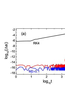
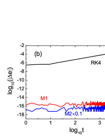
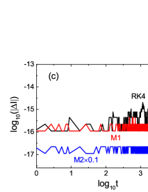
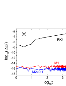
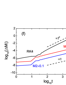
Figure 1: Errors of six orbital elements for the pure Keplerian orbit. The adopted algorithms are RK4 and its correction methods: the newly proposed method M1 and Fukushima’s linear transformation method M2. For M2, all errors are reduced by 10 times. The error of mean longitude $M$ increases in proportion to the square of time for RK4, whereas it linearly increases for M1 and M2. In fact, the error curve of M1 basically coincides with that of M2 in each panel.

Let us consider the Kepler problem with parameter $\mu=1$ and initial orbital elements $a_{0}=2$ AU, $e_{0}=0.3$, $I_{0}=20^{\circ}$, $\Omega_{0}=50^{\circ}$, $\omega_{0}=30^{\circ}$, and $M_{0}=40^{\circ}$. Take a conventional fourth-order Runge-Kutta algorithm (RK4) with a fixed time step $h$ being 1/100 of orbital period $T$ ($h=T/100$). In Figure 1, the new method M1 drastically reduces the integration errors of all orbital elements compared with the uncorrected algorithm RK4. The errors of the five constant orbital elements for the two projection methods M1 and M2 should be zeros from the theory. However, they may be zeros at some cases or equal to or near the machine double precision $\epsilon=10^{-16}$ at some other times from the computation. To ensure that the logarithms can work well for the zero errors in Figure 1, we add $\epsilon$ to these errors, that is, $|\Delta a|+\epsilon\rightarrow|\Delta a|$ in panel (a). The error of mean longitude $M$ increases in proportion to the square of time for the uncorrected method RK4, whereas it linearly grows with time for the corrected schemes M1 and M2. The new method M1 is approximately the same as the method M2 in controlling the accumulation of integration errors in all orbital elements.

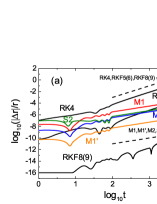
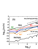
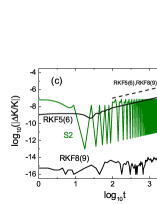
Figure 2: Same as Figure 1, but relative position errors (a) and velocity errors (b) are used rather than the errors of the orbital elements. Here, M1 is the new projection method of RK4, and M2 is Fukushima’s method of RK4. RKF5(6), its new correction scheme M1’, RKF8(9) and symplectic integrator S2 are added. The position or velocity errors linearly grow with time for the projection methods M1, M2 and M1’ and S2, whereas they linearly grow with a law of the square of time for RK4, RKF5(6) and RKF8(9). The energy errors in (c) linearly grow for RKF5(6) and RKF8(9), but remain at the machine precision level for the projection methods (not plotted) and are bounded for S2.

The two correction methods have the same performance in suppressing the errors in the positions and velocities, as shown in Figures 2(a) and 2(b). The rates of error growth in the velocities and positions for RK4 and its correction methods M1 and M2 are the same as those in the mean longitudes for the corresponding algorithms. Here, the estimations of the errors in the mean longitudes, positions and velocities use the analytical solutions. The analytical solutions from Equations (16) and (17) are approximately the same as those given by the Kepler solver of Wisdom $\&$ Hernandez (2015) or Rein $\&$ Tamayo (2015). When time $t=10^{6}$ corresponding to $10^{8}$ steps ($h=0.01$ in this case but $h=T/100$ in Figure 2), the Kepler solver of Wisdom $\&$ Hernandez and the analytical solution method given by Equations (16) and (17) consume 28.5 and 26.8 s CPU times, respectively. This finding indicates that the difference in computational effort between the two analytical solvable methods is small.

The pure two-body problem is a good material to test the numerical performance of an integrator because it contains known analytical solutions. The proposed projection method is verified in the above experiments using RK4 as a basic integrator. To satisfy the later need, we continue to use the Kepler problem to test other numerical integration algorithms, including a five- and six-order Runge-Kutta-Fehlberg algorithm [RKF5(6)] with a fixed step size, its new projection method M1’, an eighth- and ninth-order Runge-Kutta-Fehlberg algorithm [RKF8(9)] with variable step sizes and a second-order symplectic integrator S2.

The symplectic method requires that Equation (1) be split into two parts

$$K=H_{0}+H_{1},~{}~{}H_{0}=\frac{v^{2}}{2}-\frac{0.999}{r},~{}~{}H_{1}=-\frac{0.001}{r}.$$ (35)

$H_{0}$ is still a main Kepler part, and $H_{1}$ is a small perturbation part. They are independently and analytically solvable. The splitting method is slightly similar to that of Wisdom $\&$ Holman (1991). Let $\mathcal{A}$ be an operator for analytically solving $H_{0}$ and $\mathcal{B}$ be as another operator for analytically solving $H_{1}$. This method is simply written in the form

$$S2=\mathcal{B}(\frac{h}{2})\circ\mathcal{A}(h)\circ\mathcal{B}(\frac{h}{2}).$$ (36)

The ratio of the mass for $H_{1}$ to the mass for $H_{0}$, $\varepsilon=1/999$, approaches that of the largest planet’s mass to the Sun’s mass in the solar system. Such a splitting Hamiltonian technique will give the established algorithm (29) a better accuracy than the usually splitting method with the kinetic energy plus the potential energy. This finding is because the former truncation energy error is $\mathcal{O}(\varepsilon h^{2})$ and the latter one is $\mathcal{O}(h^{2})$.

The algorithms about the relative position or velocity errors from the smallest to the largest in Figures 2(a) and 2(b) are RKF8(9), the new correction method M1’ of RKF5(6), S2, M1 (or M2) of RK4, RKF5(6) and RK4. The energy errors in panel (c) remain bounded for S2 because S2 shares an advantage of preserving simplecticity. The energy errors of RKF8(9) are the smallest but grow with time. The energy errors of RKF5(6) also grow. This error growth is because the non-symplecticity of the two algorithms results in the long-term accumulation of roundoff errors. After $t=1000$ corresponding to 5882 steps, RKF5(6) becomes poorer than S2; this result can also be observed from the position or velocity errors. The two projection methods consistently make the energy errors (not plotted) arrive at the machine precision.

A simple analysis is provided to the rate of error growth for each of the above algorithms. As claimed by Rein $\&$ Spiegel (2015), the total error of an integrator comes from four contributions

$$E_{tot}=E_{fl}+E_{rand}+E_{bias}+E_{tr}.$$ (37)

In the above equation, $E_{fl}$ relates to a computer giving any calculation a relative error of approximately $2\times 10^{-16}$ in the double floating-point precision, that is, $E_{fl}\propto W\times 10^{-16}$ ($W$ being the number of computations). $E_{rand}$ is a random error from any calculation involving two random floating-point numbers. The random Kepler energy error will grow as $\propto t^{1/2}$, and the random phase errors (e.g. the mean longitude error or the position error) grow as $\propto t^{3/2}$ for any integrator. $E_{bias}$ represents an error caused by floating-point operations with respect to some specific functions, such as square root, sine or cosine functions. The errors, namely, $E_{bias}\propto t$ for the Kepler energy error or $\propto t^{2}$ for the phase error, might be biased and grow with time. The three error contributions depend on floating-point numbers and are inherent to all integrators. They are usually called roundoff errors. In addition, $E_{tr}$ is an error associated with the integrator itself and is also called a truncation error. The truncation error is $E_{tr,phase}=\mathcal{O}(\frac{h}{T})^{j+1}$ in the phase (solution) and reads $E_{tr,energy}=\mathcal{O}(\frac{h}{T})^{j}$ in the energy (Hamiltonian) when the integrator is accurate to an order $j$.

Table 1 of Rein $\&$ Spiegel (2015) showed that the Kepler energy error grows as $\propto t$ and the phase error does as $\propto t^{2}$ for RK4. This fact can be also clearly observed from the errors of the semimajor axis and mean anomaly in Figures 1(a) and 1(f) and from the errors of the positions and velocities in Figures 2(a) and 2(b). The rates of phase error growth with time for RK4 are similarly suited for RKF5(6) and RKF8(9). However, some differences are found. The truncation phase error of RKF5(6) with an order of $\mathcal{O}(\frac{h}{T})^{6}$ is smaller than that of RK4 with an order of $\mathcal{O}(\frac{h}{T})^{5}$ and that of RKF8(9) is the smallest. In particular, the truncation phase error of RKF8(9) is $\sim\mathcal{O}(\frac{h}{T})^{9}=\mathcal{O}(\frac{1}{100})^{9}=\mathcal{O}(10^{-18})$ when a constant step-size is given. The error is difficult to estimate because RKF8(9) adopts adaptive time-steps. However, Figure 2 (a) shows that RKF8(9) approximately makes the position errors remain at the machine precision until $t=10$. This finding indicates that the truncation error can be negligible. Although RFK8(9) has an extremely high precision, it still causes the Kepler energy error to linearly grow with time and the phase error to grow as $\propto t^{2}$, similar to IAS15 of Rein $\&$ Spiegel (2015). In addition, this table shows that S2 maintains a bounded energy error. This result is also shown in Figure 2 (c). In the table, the phase error is zero when the floating-point precision and implementation specific errors are ignored. However, the results under the existence of these errors in Figures 2(a) and 2(b) show that the position or velocity errors grow linearly with time for S2. The rates of phase error growth for S2 are also the same for the projection methods M1 of RK4, M2 of RK4 and M1’ of RKF5(6).

To show the phase error growth of these algorithms, we use Equations (25) and (26) to estimate the position and velocity errors in accordance with the following forms

$$\Delta\textbf{r}^{*} = a_{0}\Delta E^{*}(-\frac{\sin E^{*}}{e_{0}\mu}\textbf{P}_{0}+\sqrt{1-e^{2}_{0}}\cos E^{*}\textbf{Q}_{0}),$$ (38)

$$\Delta\textbf{v}^{*} = -\frac{a^{2}_{0}n_{0}}{r^{*}}\Delta E^{*}(\frac{\cos E^{*}}{e_{0}\mu}\textbf{P}_{0}+\sqrt{1-e_{0}^{2}}\sin E^{*}\textbf{Q}_{0})$$ (39)

$$+\frac{a^{3}_{0}n_{0}}{r^{*2}}(\frac{\sin E^{*}}{e_{0}\mu}\textbf{P}_{0}-\sqrt{1-e_{0}^{2}}\cos E^{*}\textbf{Q}_{0})$$

$$\cdot e_{0}\sin E^{*}\Delta E^{*},$$

where $\Delta E^{*}$ is calculated in terms of the Kepler equation by

$$\Delta E^{*}=\frac{\Delta n^{*}}{1-e_{0}\cos E^{*}}t=-\frac{3}{\mu}\frac{(-2K)^{1/2}\delta K}{1-e_{0}\cos E^{*}}t.$$ (40)

Then, we have

$$|\Delta\textbf{r}^{*}| \leq \frac{3a_{0}}{\mu}\frac{(-2K)^{1/2}}{1-e_{0}}(\frac{1}{e_{0}\mu}+\sqrt{1-e^{2}_{0}}~{})|\Delta K|t,$$ (41)

$$|\Delta\textbf{v}^{*}| \leq \frac{3a^{2}_{0}e_{0}n_{0}}{\mu(1-e_{0})}(\frac{1}{e_{0}\mu}+\sqrt{1-e_{0}^{2}}+\frac{1}{a_{0}(1-e_{0})e_{0}\mu}$$ (42)

$$+\frac{1}{a_{0}(1-e_{0})}\sqrt{1-e_{0}^{2}}~{})\frac{(-2K)^{1/2}}{1-e_{0}}|\Delta K|t.$$

For the projection methods, $|\Delta K|=0$ from the theory, whereas $|\Delta K|\neq 0$ (such as $|\Delta K|\sim 10^{-16}$) because of the floating-point precision and implementation specific errors. Consequently, the projection methods lead to a linear increase of the phase errors. Although eccentric anomaly $E^{*}$ is obtained from Equations (23) and (24) rather than the Kepler equation, the new projection method will consistently force $E^{*}$ in Equations (23) and (24) to satisfy the Kepler equation.

Equations (34) and (35) are useful to explain the linearly increasing phase errors of a symplectic integrator (e.g. S2) in accordance with the boundness of $|\Delta K|$, that is, $|\Delta K|\leq C$. In addition, they can explain why the phase errors grow with $t^{2}$ for a non-symplectic integrator, such as RK4. This is because the energy errors $|\Delta K|$ for this algorithm grow linearly with $t$, that is, $|\Delta K|\propto t$.

Which error dominates is difficult to answer. Its answer requires the consideration of different things in different contexts. In addition to this, several facts can be concluded from the above theoretical analysis and numerical checks. The newly proposed method is extremely successful to rigorously conserve the seven integrals in the pure Kepler problem. It can intensively suppress the rapid accumulation of the integration errors in all orbital elements and cause the phase errors to linearly grow with time. The proposed method is approximately the same as Fukushima’s method in two points. The application of the proposed method to quasi-Keplerian motions of perturbed two-body or $N$-body problems will be discussed in the next sections.

3 Perturbed two-body problems

In this section, we mainly focus on the application of the proposed method in calculating the quasi-Keplerian orbits of perturbed two-body problems. Some details of the implementation of the proposed method are described. The numerical performance of the new method is evaluated using two models of quasi-Keplerian motions, namely, a post-Newtonian two-body problem and a dissipative two-body problem.

For the two-body problem with a small perturbation, Equation (2) becomes

$$\frac{d\textbf{v}}{dt}=-(\frac{\mu}{r^{3}})\textbf{r}+\textbf{a},$$ (43)

where a is a perturbed acceleration. This perturbed two-body problem is also called the quasi-Keplerian problem. In this case, the Kepler energy, angular momentum vector and LRL vector in Equations (1), (4) and (5) are no longer invariant and slowly vary with time. Thus, the application of the new method becomes difficult.

3.1 Integral invariant relations

Kepler energy $K^{\ast}$, angular momentum vector $\textbf{L}^{\ast}$ and LRL vector $\textbf{P}^{\ast}$ are slowly-varying quantities. They satisfy the following relations

$$\frac{d\Delta K^{\ast}}{dt} = \mathbf{v}\cdot\mathbf{a},$$ (44)

$$\frac{d\Delta\mathbf{L}^{\ast}}{dt} = \mathbf{r}\times\mathbf{a},$$ (45)

$$\frac{d\Delta\mathbf{P}^{\ast}}{dt} = 2(\mathbf{v}\cdot\mathbf{a})\mathbf{r}-(\mathbf{r}\cdot\mathbf{a})\textbf{v}-(\mathbf{r}\cdot\mathbf{v})\mathbf{a}.$$ (46)

Note that $\Delta K^{\ast}=K^{\ast}-K_{0}$, $\Delta\textbf{L}^{\ast}=\textbf{L}^{\ast}-\textbf{L}_{0}$, and $\Delta\textbf{P}^{\ast}=\textbf{P}^{\ast}-\textbf{P}_{0}$, where $K_{0}$, $\textbf{L}_{0}$ and $\textbf{P}_{0}$ are the starting values of these slowly-varying quantities. Taking zeros as the initial values of $\Delta K^{\ast}$, $\Delta\textbf{L}^{\ast}$ and $\Delta\textbf{P}^{\ast}$ can immensely reduce the roundoff errors in numerical integrations. Equations (37)-(39) are integral invariant relations of the slowly-varying quantities (Szebehely $\&$ Bettis 1971).

Equations (36)-(39) are integrated. Thus, a numerical solution $(\textbf{r}^{\star},\textbf{v}^{\star})$ is obtained. At the same time, a set of values of the slowly-varying quantities $K^{*}$, $\textbf{L}^{*}$ and $\textbf{P}^{*}$ are also given. In addition to them, another set of values $K^{\star}$, $\textbf{L}^{\star}$ and $\textbf{P}^{\star}$ can be given to these slowly-varying quantities when the numerical solution $(\textbf{r}^{\star},\textbf{v}^{\star})$ is directly substituted into Equations (1), (4) and (5). Which of the two sets of values from the two different paths are more accurate? The $K^{*}$, $\textbf{L}^{*}$ and $\textbf{P}^{*}$ values from the integral invariant relations are. As indicated in (Huang $\&$ Innanen 1983), numerical solutions consistently keep each integral constant as much as possible. Because the numerical solutions $K^{*}$, $\textbf{L}^{*}$ and $\textbf{P}^{*}$ directly come from the numerical integration of Equations (37)-(39), they naturally have higher accuracies than the $K^{\star}$, $\textbf{L}^{\star}$ and $\textbf{P}^{\star}$ values calculated by the coordinates and velocities $(\textbf{r}^{\star},\textbf{v}^{\star})$. This fact has been confirmed via many successful examples of manifold correction to conservative, nonconservative or dissipative systems (Fukushima 2003a, 2003b, 2003c, 2004; Wang et al. 2016; Wang et al. 2018).

3.2 Implementation of the proposed method

Using the above $K^{*}$, $\textbf{L}^{*}$ and $\textbf{P}^{*}$ values from the integral invariant relations, we obtain the five slowly-varying orbital elements $a^{*}$, $e^{*}$, $I^{*}$, $\Omega^{*}$ and $\omega^{*}$ with mean motion $n^{*}$. Then, $a_{0}$, $e_{0}$, $I_{0}$, $\Omega_{0}$, $\omega_{0}$ and $n_{0}$ in Equations (20), (21) and (23)-(27) are the values at the beginning of each step integration rather than those at the initial time. They are replaced with $a^{*}$, $e^{*}$, $I^{*}$, $\Omega^{*}$, $\omega^{*}$ and $n^{*}$, respectively. $\textbf{L}_{0}$ and $\textbf{P}_{0}$ in Equation (22) should also give place to $\textbf{L}^{*}$ and $\textbf{P}^{*}$. In this way, the new correction scheme M1 given by Equations (25) and (26) can still work in the perturbed case. Angles $\Omega^{*}$, $I^{*}$ and $\omega^{*}$ are not necessarily known, but only their sines and cosines. Such an operation is helpful to save computational cost and to reduce the roundoff errors.

Summarised from the above demonstrations, the implementation of the new method in the present case is described as follows.

At an $i$th step, integrate Equations (36)-(39) using a certain numerical integrator and obtain the values $\textbf{r}^{\star}$, $\textbf{v}^{\star}$, $K^{*}$, $\textbf{L}^{*}$ and $\textbf{P}^{*}$.

Calculate the values $a^{*}$, $e^{*}$, $I^{*}$, $\Omega^{*}$, $\omega^{*}$ and $n^{*}$ in terms of $K^{*}$, $\textbf{L}^{*}$ and $\textbf{P}^{*}$.

Give the cosine and sine of eccentric anomaly $E^{*}$ using Equations (23) and (24).

Obtain the corrected numerical solution $(\textbf{r}^{*},\textbf{v}^{*})$ from Equations (25) and (26) with $a^{*}\rightarrow a_{0}$, $e^{*}\rightarrow e_{0}$, $I^{*}\rightarrow I_{0}$, $\Omega^{*}\rightarrow\Omega_{0}$, $\omega^{*}\rightarrow\omega_{0}$ and $n^{*}\rightarrow n_{0}$.

Take $\textbf{r}^{*}\rightarrow\textbf{r}^{\star}$ and $\textbf{v}^{*}\rightarrow\textbf{v}^{\star}$, and let a next step integration begin.

3.3 Post-Newtonian two-body problem

Let us consider a relativistic two-body problem with first-order post-Newtonian corrections (Newhall et al. 1983) as a test example of the perturbed quasi-Keplerian problems. It corresponds to the equations of motion

$$\ddot{\textbf{r}} = -\frac{\mu}{r^{3}}\textbf{r}+\mathbf{a}_{PN},$$ (47)

$$\mathbf{a}_{PN} = \frac{\mu}{c^{2}}[(\frac{4\mu}{r}-v^{2})\frac{\textbf{r}}{r^{3}}+4\frac{\textbf{r}\cdot\textbf{v}}{r^{3}}\textbf{v}],$$

where $c$ is the velocity of light, and $\mathbf{a}_{PN}$ is a perturbed acceleration from the post-Newtonian contributions. Such an equation is derived from a first-order post-Newtonian Lagrangian approach $\ell$ and truncates second-order and higher-order post-Newtonian terms.

Although Equation (40) should conserve a conservative energy, this conservative energy has no way to be exactly written in a detailed expressional form. A conservative energy of the form $\mathcal{E}(\textbf{r},\textbf{v})=\textbf{v}\cdot\mathbf{\wp}-\ell$, where $\mathbf{\wp}=\partial\ell/\partial\textbf{v}$ is a generalised momentum, can be conserved approximately using Equation (40). However, energy $\mathcal{E}$ can be conserved strictly using equation $\mathbf{\dot{\wp}}=\partial\ell/\partial\textbf{r}$ with $\mathbf{v}$ given by $\mathbf{\wp}=\partial\ell/\partial\textbf{v}$. It is called as a coherent post-Newtonian Lagrangian equation (Li et al. 2019; Li et al. 2020). Such a coherent equation is different from Equation (40) because no terms are truncated when the coherent equation is derived from the Lagrangian $\ell$. However, some post-Newtonian terms must be truncated when Equation (40) is obtained from $\ell$. This condition explains why the coherent equation can exactly conserve energy $\mathcal{E}$ but Equation (40) can approximately do.

Equation (40) also approximately conserves a conservative Hamiltonian $\mathcal{H}(\textbf{r},\mathbf{\wp})=\textbf{v}\cdot\mathbf{\wp}-\ell$. The two formulations $\ell$ and $\mathcal{H}$ are not exactly equivalent (Wu et al. 2015; Wu $\&$ Huang 2015). $\mathcal{E}$ and $\mathcal{H}$ are not either. This condition indicates that Equation (40), coherent equation and system $\mathcal{H}$ are three different dynamical problems. These differences among them are negligible for the weak gravitational solar system, and the three dynamical systems are approximately the same. However, the differences are large for a strong gravitational field of compact objects, and the three dynamical systems are approximately related. Considering that Equation (40) cannot exactly conserve energy $\mathcal{E}$, conserving the Kepler energy in Equation (1) is impossible. The LRL vector in Equation (5) is not invariant. In addition, the Newtonian angular momentum given by velocity $\mathbf{v}$ in Equation (4) is not constant, whereas the angular momentum $\textbf{r}\times\mathbf{\wp}$ defined by momentum $\mathbf{\wp}$ is constant. The constant angular momentum makes the orbital plane invariable. The motion is limited to the plane because the post-Newtonian effect is given in the invariable orbital plane. In this case, inclination $I$ and longitude of ascending node $\Omega$ are not affected by the post-Newtonian effect and remain invariant. However, the other orbital elements $a$, $e$ and $\omega$ are affected and slowly vary with time.

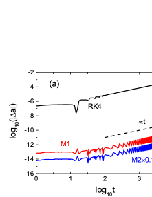
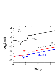
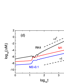
Figure 3: Errors of elements $a$, $e$, $\omega$ and $M$ for the post-Newtonian two-body problem. The accuracies of $a$, $e$ and $\omega$ for the two correction schemes M1 and M2 are typically improved by 6 and 7 orders of magnitude, but cannot remain on the machine precision because the post-Newtonian effect makes the three elements vary with time. The errors of $M$ are reduced by several orders of magnitude.

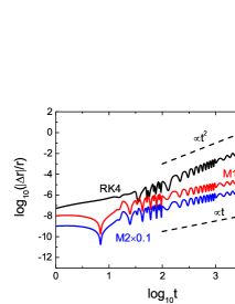
Figure 4: Same as Figure 3 but relative position errors are used rather than the errors of the elements. The error growth is linear for M1 and M2, but is a quadratic function of time for RK4.

Here, RK4 is still used as a basic integrator. We take parameter $\mu=1$ and a fixed step size $h=T/120$, where $T$ is an orbital period. The initial orbital elements are $a=2$ AU, $e=0.1$, $I=20^{\circ}$, $\Omega=50^{\circ}$, $\omega=30^{\circ}$, and $M=40^{\circ}$. The speed of light $c=10^{4}$ corresponds to the first-order post-Newtonian effect, which is approximate to an order of $10^{-8}$ (compared with the main Kepler part) in the solar system (Dubeibe et al. 2017; Huang et al. 2018). The correction methods M1 and M2 can naturally preserve the two constant elements $I$ and $\Omega$ because the conserved angular momentum is strictly kept in the manifold corrections. In Figure 3, the errors of the varying elements $a$, $e$ and $\omega$ for the two correction schemes are decreased by 6 and 7 orders of magnitude compared with those for RK4. In addition, the errors of $M$ are reduced by 3 orders of magnitude. Thus, the relative position errors in Figure 4 are reduced. Considering that RKF8(9) shows extremely good accuracy in the above two-body problem under the circumstance of roundoff errors ignored, it is still used to give the post-Newtonian problem high-precision reference solutions to obtain the various errors in Figures 3 and 4. The high-precision solutions can also be given by IAS15 of Rein $\&$ Spiegel (2015).

We discuss why such a more accurate eccentric anomaly $E^{*}$ is calculated in terms of Equations (23) and (24). Four possible choices can be used in the calculation of $E^{*}$.

Case 1, a naturally prior choice is to solve $E^{*}$ from the Kepler equation (14). The Kepler equation reads

$$E^{*}_{i}-e^{*}_{i}\sin E^{*}_{i}=M^{*}_{i-1}+n^{*}_{i-1}\Delta t,$$ (48)

where $\Delta t$ is a time step and $M^{*}_{i-1}$ denotes the value of $M$ at the $(i-1)$th step. This path for the computation of $E^{*}$ is marked as C1.

Case 2, mean motion $n^{*}_{i-1}$ in Equation (41) takes an average value of $n^{*}_{i-1}$ at the $(i-1)$th step and $n^{*}_{i}$ at the $i$th step; namely, $\bar{n}^{*}_{i-1}=(n^{*}_{i-1}+n^{*}_{i})/2$ because the mean motion is not invariant. In this case, the Kepler equation is

$$E^{*}_{i}-e^{*}_{i}\sin E^{*}_{i}=M^{*}_{i-1}+\bar{n}^{*}_{i-1}\Delta t.$$ (49)

The computation of $E^{*}$ is marked as C2.

Case 3, calculate $E^{*}$ with the numerical solution $(\textbf{r}^{\star},\textbf{v}^{\star})$, that is,

$$\cos E^{*}=\frac{a^{*}-r^{\star}}{e^{*}a^{*}},~{}~{}\sin E^{*}=\frac{\textbf{r}^{\star}\cdot\textbf{v}^{\star}}{e^{*}n^{*}a^{*2}}.$$ (50)

The method for computing $E^{*}$ is marked as C3.

Case 4, calculate $E^{*}$ using Equations (23) and (24). The computation of $E^{*}$ along this direction is still marked as M1.

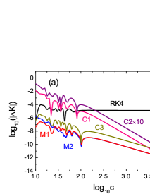
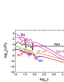
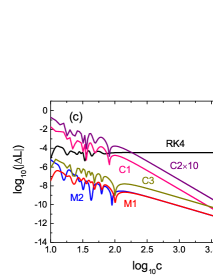
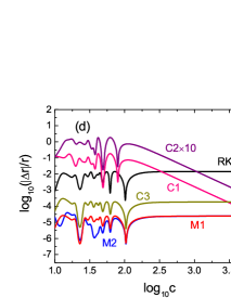
Figure 5: Dependence of errors of $K$, $|\textbf{L}|$, $|\textbf{P}|$ and $|\textbf{r}|$ on the value of $c$ in the post-Newtonian two-body problem. The variation of $c$ indicates that of the perturbation. Four choices labelled as C1, C2, C3 and M1 can be used for the calculation of the eccentric anomaly. M1 is the best choice for various values of $c$.

Let $c$ range from 10 to $10^{4}$ at an interval of 2. This condition indicates that the perturbation varies from strong to weak and is approximately at an interval of [$10^{-8}$, $10^{-2}$]. For a given value of $c$, the related errors in each of the four cases are shown in Figure 5. In the numerical performance, C1 and C2 or M1 and M2 have no explicit differences. When the perturbation is extremely small for $c=10^{4}$, C1 is approximately consistent with M1. C1 becomes poorer than M1 with the increase in perturbation and is inferior to the uncorrected method RK4 when $c=30$. These tests show that the obtainment of $E^{*}$ from Equations (23) and (24) is the best choice. This result is typically suitable for the quasi-Keplerian motions in the solar system because the perturbation of each planet is approximately in an interval of $(10^{-5},10^{-3})$ compared with the individual Kepler part.

3.4 Two-body problem with dissipative force

As discussed in the Introduction, the velocity scaling method of Ma et al. (2008b) combined with the integral invariant relation worked well in nonconservative or dissipative systems (Wang et al. 2016, 2018). What about the new correction method M1 applied to dissipative systems?

To answer this question, we take the dissipative two-body problem considered by Tamayo et al. (2019)

$$\frac{d\textbf{v}}{dt}=-(\frac{\mu}{r^{3}})\textbf{r}+\mathbf{a}_{d},~{}~{}\mathbf{a}_{d}=-\gamma\mathbf{v},$$ (51)

where $\gamma$ is a damping parameter, and $\mathbf{a}_{d}$ is a perturbed acceleration from a damping force. In this case, the Kepler energy (1) is not a conserved quantity. Taking the damping factor $\gamma=2\times 10^{-6}$ and the same initial conditions and step size $h$ in the above post-Newtonian problem, we still adopt RK4 and its correction scheme M1 to solve the dissipative system (44). In addition, we use a fourth-order implicit method with a symmetric combination of three second-order implicit midpoint methods

$$IM4=IM2(\lambda h)\circ IM2((1-2\lambda)h)\circ IM2(\lambda h),$$ (52)

where $\lambda=1/(2-\sqrt[3]{2})$. This construction is based on the idea of Yoshida (1990). IM2 and IM4 are symplectic when they are applied to integrate a Hamiltonian. High-precision reference solutions are still given by RKF8(9).

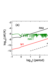
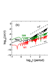
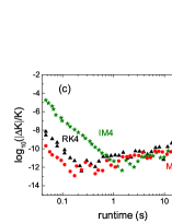
Figure 6: Relative errors of the Kepler energy (a) and position (b) in the dissipative two-body problem. The parameters, initial conditions and step-size are the same as those (except $e=0.3$) in Figure 3. M2 is not considered, and the fourth-order implicit symplectic method IM4 is used for comparison. When the time is measured in units of unperturbed period $T$ in panels (a) and (b), the integration time $t=10^{5}$ is $5630~{}T$. (c) Efficiencies for the description of dependence of relative energy errors on the computer runtime. Each point corresponds to the energy error after integration time $t=10^{4}$ (i.e. $563~{}T$). For a given runtime, the three algorithms use different fixed step sizes.

As shown in Figures 6(a) and 6(b), the relative errors in the Kepler energy and position are several orders of magnitude smaller for M1 than those for RK4 before the integration time $t=10^{5}$ corresponding to $5630~{}T$, where $T$ is the unperturbed period. The correction method M1 is superior to the fourth-order implicit method IM4 in the accuracy. The energy errors for IM4 have a secular growth with integration because of the dissipative force or roundoff errors. The relative position errors grow as $\propto t^{2}$ for RK4, but $\propto t$ for M1 and IM4.

The efficiency regarding the dependence of the relative energy errors on the computer runtime for each algorithm with integration time $t=10^{4}$ (i.e. $563~{}T$) is plotted in panel (c). The algorithms RK4, M1 and IM4 use different large fixed time steps $0.0066\times 563T/10000$, $0.013\times 563T/10000$ and $0.041\times 563T/10000$, respectively, when a short runtime (e.g. 0.1s) is given. Clearly, the algorithms with the computational speeds from fast to slow are RK4, M1 and IM4. The algorithms from high accuracies to low ones are M1, RK4 and IM4. The time step of IM4 is larger than those of RK4 and M1. This is an important reason for IM4 obtaining the poorest accuracies. In terms of efficiency, an integrator that costs less CPU time has better efficiency compared with another integrator for a given accuracy. On this basis, the efficiencies from good to poor are M1, RK4 and IM4 for the short runtimes considered. The algorithms have to adopt different small fixed time steps, such as $h=0.000083\times 563T/10000$ for RK4, $h=0.00014\times 563T/10000$ for M1 and $h=0.00039\times 563T/10000$ for IM4 when a long runtime (e.g. 8 s) is given. This condition leads to increasing the number of integration steps and the fast accumulation of roundoff errors for each integrator. In this case, the three methods have no explicit differences in the efficiencies.

4 Multi-body problems

In this section, we focus on the application of the proposed method to a five-body problem of the Sun and four outer planets. For comparison, the Wisdom-Holman method and a fourth-order symplectic integrator of Yoshida (1990) are considered.

Suppose each planet of an $N$-body gravitational problem in the solar system moves in a quasi-Keplerian orbit. In the barycentre coordinate system, this problem is described by the following Hamiltonian

$$H=\sum^{N-1}_{j=0}\frac{\mathbf{p}^{2}_{j}}{2m_{j}}-\sum^{N-2}_{s=0}\sum^{N-1}_{j>s}\frac{Gm_{s}m_{j}}{r_{sj}}.$$ (53)

$j=0$ denotes the Sun, and $j=1,2,\ldots$ correspond to various planets. The $j$th object has mass $m_{j}$, position coordinate $\mathbf{r}_{j}$ and momentum $\mathbf{p}_{j}$. This system has seven conservative integrals, involving the total energy $E$, total momentum vector p and total angular momentum vector L:

$$E = H,$$ (54)

p $$= \sum^{N-1}_{j=0}\textbf{p}_{j},$$ (55)

L $$= \sum^{N-1}_{j=0}\textbf{r}_{j}\times\textbf{p}_{j}.$$ (56)

They all are independent in the $N$-body system. They are also in the two-body problem in the barycentre coordinate system. However, the three integrals on the momenta are missing and the three integrals of the LRL vector are included in the relative coordinate system. Only five integrals are independent in this case, as previously indicated.

Hairer et al. (1999) reported that a five-body integration of the Sun and four outer planets shows poor numerical performance when the total energy and total angular momenta are rigorously preserved through a projection method. However, the corrections of individual Kepler energies, angular momenta and LRL vectors work well in a heliocentric coordinate system (Fukushima 2003a, 2003b, 2003c, 2004; Wu et al. 2007; Ma et al. 2008a, 2008b). Naturally, the application of the new correction scheme to such an $N$-body problem should be considered.

In the heliocentric coordinate system, each planet relative to the Sun has position vector $\mathbf{\tilde{r}}_{j}$ and velocity vector $\mathbf{\tilde{v}}_{j}$ ($j=1,2,\ldots,N-1$). The evolution equation of the quasi-Keplerian motion of each body is still similar to Equation (36), where the perturbed acceleration is expressed as

$$\mathbf{\tilde{a}}_{j}=\sum^{N-1}_{s=1,\neq j}Gm_{s}(\frac{\mathbf{\tilde{r}}_{s}-\mathbf{\tilde{r}}_{j}}{|\mathbf{\tilde{r}}_{s}-\mathbf{\tilde{r}}_{j}|^{3}}-\frac{\mathbf{\tilde{r}}_{s}}{\tilde{r}^{3}_{s}}).$$ (57)

Therefore, the new method M1 fitting for the perturbed two-body problems is applied to the quasi-Keplerian motions of individual planets in the multi-body problem.

Taking a five-body problem consisting of the Sun and four outer planets (Jupiter, Saturn, Uranus and Neptune) as an example, we consider the application of the new method M1 to this problem. All data are taken from those in the ephemerides DE431. RK4 uses a fixed step-size $h=36.525$ days, which is approximately 1/120 of the orbital period $T$ of Jupiter. For comparison, the second-order symplectic integrator of Wisdom $\&$ Holman (1991) is included. We call it the WH method. The use of WH and its extensions (e.g. Hernandez $\&$ Dehnen 2017) requires that the Hamiltonian with $N=5$ in Equation (46) have an appropriate splitting form similar to Equation (28). In the Jacobi coordinate system, the Kepler part $H_{0}$ and the planet-planet interaction part $H_{1}$ can be obtained. The ratio of the latter part to the former part is approximately 1/1047. In this way, the WH integrator similar to S2 in Equation (29) becomes easily available.

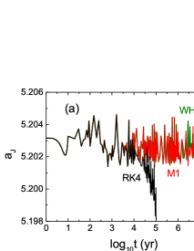
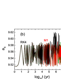
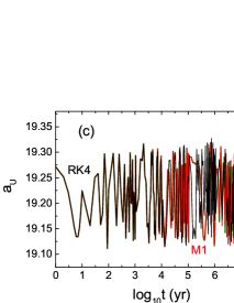
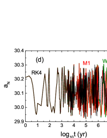
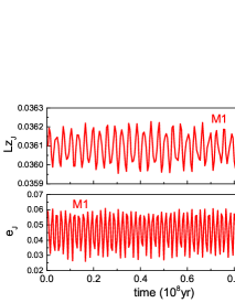
Figure 7: Evolution of some orbital elements and quasi-integrals in the five-body problem of the Sun and outer planets. The algorithms are RK4 and its correction method M1. The WH method is used for comparison. Semi-major axis $a$ of Jupiter in panel (a) and eccentricity $e$ and $z$-direction angular momentum $L_{z}$ of Jupiter in panel (e) decay with time for RK4 but remain bounded by M1 (similar to WH) until integration time $t$ reaches $10^{8}$ years in panels (a) and (f).

Figure 7 plots the evolution of some orbital elements and quasi-integrals in the five-body problem. Clearly, RK4 gives a secular change to the semi-major axis $a$ of Jupiter in an integration time of $10^{5}$ years in Figure 7 (a). The semi-major axis decreases to 5.198 AU in the integration time. Such similar changes are also given to eccentricity $e$ and $z$-direction angular momentum $L_{z}$ of Jupiter in an integration time of $10^{7}$ years in Figure 7 (e). However, no secular changes are found in other orbital elements and quasi-integrals (including those not plotted). Fortunately, the secular changes can be eliminated using the projection method M1 (similar to WH) in Figures 7(a) and 7(f). In particular, the semi-major axis $a$, eccentricity $e$ and angular momentum $L_{z}$ of Jupiter remain bounded until integration time $t$ reaches $10^{8}$ years. For example, the semi-major axis is consistently limited to a bounded region between 5.201 and 5.205 AU during the integration time by M1, which is similar using WH. Similarly, M1 forces the three other planets’ semi-major axes to stay at bounded regions: $a_{S}\approx 9.51-9.59$ AU for Saturn, $a_{U}\approx 19.10-19.31$ AU for Uranus and $a_{N}\approx 29.90-30.35$ AU for Neptune. In other words, the energies between the Sun and planets ($E_{SJ}$, $E_{SS}$, $E_{SU}$ and $E_{SN}$) in the barycentre coordinate system are bounded because of the relation (8). As shown in Figure 7, the secular changes that exist in some elements or quasi-integrals for RK4 adopting short integration times are absent in M1 with long integration times. This fact sufficiently shows the advantage of the new projection method in typically suppressing the error growth.

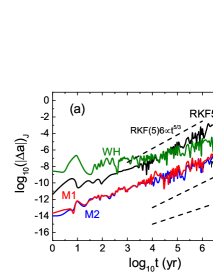
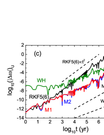
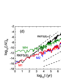
Figure 8: Same as Figure 7 but errors of some orbital elements for the other outer planets. RKF5(6) is used rather than RK4, and Fukushima’s method M2 is added. RKF8(9) is taken as a reference integrator to provide high-precision solutions. (a) Semi-major axis $a$ of Jupiter, (b) eccentricity $e$ of Saturn, (c) argument of perihelion $\omega$ of Uranus and (d) inclination $I$ of Neptune. When $t\approx 10^{6}$ years, M2 begins to become worse. At this time, errors $\Delta a$ of the semi-major axis of Jupiter remain invariant at 0.001 for RKF5(6) in panel (a), whereas they tend to this value for M1 and WH as $t$ arrives at $10^{8}$ years.

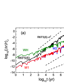
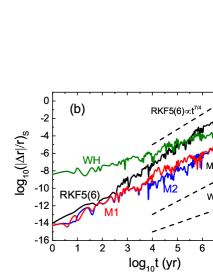
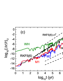
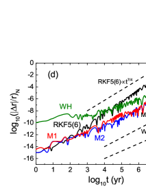
Figure 9: Same as Figure 8 but relative position errors of the outer planets. (a) Jupiter, (b) Saturn, (c) Uranus and (d) Neptune. When $t\approx 10^{6}$ years, M2 begins to become worse. At this time, the relative position errors in panel (a) are stabilised at 0.01 for RKF5(6). The other errors also tend to this value for RKF5(6), M1 and WH as $t$ reaches $10^{8}$ years.

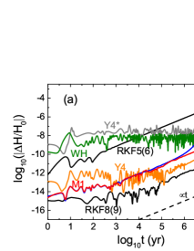
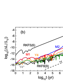
Figure 10: Same as Figure 8 but relative errors of total energy and total angular momenta in the barycentre coordinate system. Y4 is the fourth-order symplectic method of Yoshida, consisting of three WH methods. WH, Y4, RKF5(6) and its projection methods M1 and M2 use a small time step $h=36.525$ days, whereas Y4* adopts a large time step $h$*=350 days. The WH method conserves the total energy but does not conserve the total angular momenta because of roundoff errors. The energy errors are not bounded for Y4 adopting the small time-step, whereas are for Y4* adopting the large time-step. RKF8(9), M1 and M2 do not conserve the total energy. M2 begins to fail to work well when $t\approx 10^{6}$ years and is unsuitable for such a long-term integration. M1 immensely controls the rapid error growth compared with the uncorrected method RKF5(6).

Letting RK4 give place to RKF5(6), we use RKF8(9) as a high-precision reference integrator to further check the performance of the new projection method. The above secular changes to the related elements or quasi-integrals yielded by RK4 lose in each of the algorithms RKF5(6), M1, WH and RKF8(9). The above bounded regions of the four planets’ semi-major axes are also kept. Compared with the uncorrected method, the two correction schemes M1 and M2 have approximately the same performance in effectively reducing the errors from the related orbital elements until $t\approx 10^{6}$ years in Figure 8. Unfortunately, M2 begins to become worse when the integration exceeds this time, but M1 still works well before the integration time reaches $10^{8}$ years. Such similar results also occur for the relative position errors of the four planets in Figure 9 and for the relative errors of the total energy and the total angular momenta in Figure 10. The following several points can be observed from Figures 7-10.

Why do not the related errors in Figures 8 and 9 grow after some times? For instance, errors $\Delta a_{J}$ remain at 0.001 for RKF5(6) after $t\approx 10^{6}$ years and for WH after $t\approx 10^{7}$ years in Figure 8 (a). They also tend to this value for M1 as $t$ approaches $10^{8}$ years. These results are because these algorithms restrict the individual semi-major axes or energies to bounded regions. In practice, the same four significant digits 5.200 (i.e. a precision of an order of 0.001) can be given to the semi-major axis of Jupiter using the algorithms involving RKF8(9). Thus, the bounded regions or the same significant digits of the semi-major axes determine that the differences between RKF8(9) and each of RKF5(6), M1 and WH consistently remain stable at some times. The Jupiter’s relative position errors that remain stable after $10^{6}$ years in Figure 9 (a) are because they are given the same three significant digits by RKF5(6) and RKF8(9). The higher the accuracy of an algorithm is, the longer the times of the differences arriving at the stable values will be. This condition can explain why all errors in Figures 8 and 9 grow with time although the seven quasi-integrals or the five slowly-varying orbital elements of each planet are bounded in RKF5(6), M1 and WH. It also shows that WH is superior to RKF5(6) but inferior to M1.

The correction method M1 strictly satisfies the integral invariant relations of the seven slowly-varying quantities for each planet in the heliocentric coordinate system. In particular, it makes the slowly-varying orbital elements bounded or the related errors stable at some times in Figures 7-9. However, this condition does not indicate that it conserves the seven quantities because these quantities are not constant. Thus, it cannot preserve the integrals, such as total energy (47) and total angular momenta (49) in the barycentre coordinate system, as numerically shown in Figure 10. However, the total momenta (48) are conserved exactly in any algorithm because the solutions in the Jacobi coordinate system are transformed into those in the barycentre coordinate system by the conserved total momenta. The WH symplectic method can conserve the total energy but cannot conserve the total angular momenta because of roundoff errors. Although M1 and WH have difference in the conservation of the total energy, they have approximately the same effects on restricting the quasi-integrals or the slowly-varying elements to the bounded regions in Figure 7.

The preference of M1 over WH in the accuracies in Figures 7-10 sounds naturally reasonable because the order of M1 is at least 5 and that of WH is 2. To basically match with the order of M1, the Yoshida’s fourth-order explicit symplectic integrator Y4 is given by substituting WH into IM2 in Equation (45). The accuracy of Y4 has an advantage over that of M1 but is poorer than that of RKF8(9) in Figure 10. In particular, Y4 as a symplectic integrator shows a linear growth of the energy error, similar to M1 or RKF8(9). This condition is because Y4 has a truncation energy error $\mathcal{O}[\varepsilon(\frac{h}{T})^{4}]\sim\mathcal{O}[\frac{1}{1047}(\frac{1}{118.6})^{4}]\sim\mathcal{O}(10^{-12})$. When the time is $10^{5}$ years corresponding to $10^{6}$ steps, the total energy errors of Y4 can remain bounded and change between the orders of $10^{-14}$ and $10^{-11}$. If a machine error is accumulated per step, the roundoff errors grow as $\propto\frac{t}{h}\times 10^{-16}=10^{-10}$ (this result is only a rough estimation to the roundoff errors). As the integration continues, the roundoff errors cause the total energy errors of Y4 to linearly grow. The WH method can restrict the energy errors to the interval $[10^{-10},10^{-8}]$ because its truncation energy error $\mathcal{O}[\varepsilon(\frac{h}{T})^{2}]\sim\mathcal{O}[\frac{1}{1047}(\frac{1}{118.6})^{2}]\sim\mathcal{O}(10^{-8})$ is not dominated by the roundoff errors with an order of $\mathcal{O}(10^{-7})$ in the integration of $10^{8}$ years corresponding to $10^{9}$ steps. In fact, the number of integration steps for Y4 is approximately 3 times more than that for WH, and the roundoff errors become dominant after $10^{5}$ years. To suppress the fast growth of the roundoff errors, we use a large time step $h^{*}=350$ days for the fourth-order symplectic method Y4*. As expected, the total energy errors of Y4* remain bounded and are approximately consistent with those of WH with the small step size $h=36.525$ days. In this case, Y4* has a truncation energy error $\mathcal{O}[\varepsilon(\frac{h}{T})^{4}]\sim\mathcal{O}[\frac{1}{1047}(\frac{1}{11.86})^{4}]\sim\mathcal{O}(10^{-8})$, which is not governed by the roundoff errors with an order of $\mathcal{O}(10^{-8})$ in such an integration of $10^{8}$ steps. In fact, such a similar accuracy can also be yielded by the second-order WH method with symplectic correctors (Wisdom et al. 1996; Wu et al. 2003) (not plotted) for the large time step. However, the symplectic correctors need considerable computational labour because many additional iterations, such as operator $\mathcal{A}$ in Equation (29), are used. The comparison between Y4 and Y4* sufficiently shows that the roundoff errors seriously dominate the numerical errors.

In addition to the above-mentioned two points, the slopes regarding the error growth with time are different for various algorithms in Figures 8-10. They should be some combination of roundoff and truncation errors. As a high-precision reference integrator, RKF8(9) gives its truncation energy error $\mathcal{O}(\frac{h}{T})^{8}\sim\mathcal{O}(\frac{1}{118.6})^{8}\sim\mathcal{O}(10^{-17})$ when constant time step $h=36.525$ days is considered. In fact, it uses variable step-sizes, and its truncation error is difficultly estimated. As shown in Figures 2 and 10, the outputted results arrive at or approach the machine precision in short times. In this sense, the truncation errors are basically negligible for RKF8(9), and most of the errors are roundoff errors. RKF8(9), similar to IAS15 (Rein $\&$ Spiegel 2015), makes the total energy errors in Figure 10 and the phase errors grow as $t$ and $t^{2}$ because of the roundoff errors as it did in the above two-body problem. In spite of this, RKF8(9) with the truncation errors neglected can still be regarded as a reference algorithm to provide high-precision solutions in an appropriately long time.

The truncation energy error for RKF5(6) reads $\mathcal{O}(\frac{h}{T})^{5}$ $\sim$ $\mathcal{O}(\frac{1}{118.6})^{5}$ $\sim$ $\mathcal{O}(10^{-11})$. The roundoff errors for RKF5(6) lead to the total energy errors growing $\propto t$ in Figure 10 and relative position errors growing $\propto t^{2}$ in Figures 9(a) and 9(c). The position error growth is considered before the errors remain at stable values. The phase errors can be roughly observed from Equation (34). Here, $a_{j}$ and $e_{j}$ of individual planets are approximately constants. Because individual Kepler energy errors $\Delta K_{j}\propto t$ for RKF5(6), individual position errors $|\Delta\mathbf{r}_{j}|\propto t^{2}$. The projection method M1 can appropriately decrease the growth of errors $\Delta K_{j}$. Therefore, $|\Delta\mathbf{r}_{j}|\propto t^{3/2}$, as shown in Figure 9. This finding is mainly from the contribution of random errors to the phase errors of each planet, similar to that to the phase errors of the two-body problem (Rein $\&$ Spiegel 2015). The WH symplectic algorithm should make $\Delta K_{j}$ bounded if the roundoff errors are ignored. Equation (34) shows that $|\Delta\mathbf{r}_{j}|\propto t$. This result is suitable for the errors of WH in Figure 8. In a word, the slopes for the position error growth with time are WH $<$ M1 $<$ RKF5(6) before the errors tend to stable values in Figure 9. The result on WH slope $<$ M1 slope in the present case is different from the WH slope $=$ M1 slope in the two-body problem.

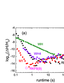
Figure 11: Same as Figure 10 but regarding efficiencies for several algorithms. Each point corresponds to the total energy error obtained after the integration time reaches $10^{4}$ years. The same runtime indicates that the algorithms (except RKF8(9)) use different fixed step-sizes. RKF8(9) with varying time-steps has only one point, corresponding to 0.45 s CPU times.

Let us measure the computational efficiencies of the algorithms RKF5(6), M1, WH, Y4 and RKF8(9). In Figure 11, the same CPU time indicates that these algorithms (except RKF8(9)) should use different fixed time steps when they independently integrate the five-body problem up to $10^{4}$ years. These methods need small computational cost when they take large step-sizes. For example, when RKF5(6), M1 and WH use the same large step-size $h=16.14$ days and Y4 uses another large step-size $h=48.23$ days, these constant step-size algorithms have approximately the same CPU time of 0.5 s. RKF8(9) has only one point, corresponding to CPU time of 0.45 s because it uses adaptive time-steps. In this case, the efficiencies from high to low are RKF8(9), M1, Y4, RK5(6) and WH. As the constant step-size methods adopt small step-sizes, they need many machine labours. Given $h=0.08$ days for RKF5(6) and WH, $h=0.1$ days for M1 and $h=0.25$ days for Y4, the constant step-size methods cost 80 s CPU times. Increasing integration steps are added, and the roundoff errors become more important than the truncation errors from the schemes because the adopted time-steps are smaller. This condition explains why the explicit differences cannot be observed among the efficiencies of the constant step-size methods when the runtime spans 30 s.

5 Summary

Using the analytical solutions of a pure two-body problem, a new projection method is proposed to rigorously conserve the seven independent and dependent integrals, including the Kepler energy, angular momentum vector and LRL vector. Unlike the analytical method that solves the eccentric anomaly from the Kepler equation with an iterative method, the newly proposed method does not need any iteration but uses the true anomaly between the constant LRL vector and a varying radial vector to obtain the eccentric anomaly. The unit radial vector is given by an integrator. In the construction mechanism, the proposed method is typically different from Fukushima’s linear transformation method for the consistency of the seven integrals. On the one hand, the former projection method does not use any scale factor, whereas the latter one uses three scale factors. On the other hand, the former corrected solutions appear to directly depend on the orbital elements rather than the numerical solutions, whereas the latter ones are typically a linear combination of the numerical solutions. Numerical simulations of the two-body problem show that the proposed method can successfully give the machine epsilon to the integration errors in all orbital elements except the mean longitude at the epoch. In addition, the proposed method and Fukushima’s method have approximately the same numerical performance. The slope of phase error growth with time for the proposed method is consistent with that for the second-order symplectic integrator.

For the quasi-Keplerian motion of a perturbed two-body problem or each body in an $N$-body problem, the seven quantities slowly vary with time. This condition is an obstacle to the application of the proposed method. We simultaneously integrate the time evolution of the seven slowly-varying quantities (called the integral invariant relations of these quantities) and the usual equations of motion. The seven quantities from the direction integration of the invariant relations are more accurate than those obtained from the integrated positions and velocities. These high-precision quantities can determine the five slowly-varying orbital elements, namely, semimajor axis, eccentricity, inclination, longitude of ascending node and argument of pericentre. The eccentric anomaly is calculated similarly using the method of the two-body problem. When these values from the integral invariant relations are substituted into the analytical solutions of the two-body problem, the solutions of the perturbed two-body problem or each planet in the $N$-body problem can be adjusted. In the expressional forms, the corrected solutions resemble the analytical solutions of the two-body problem. In this way, the proposed method can be implemented without difficulty.

The post-Newtonian two-body problem numerically confirms that the proposed method can significantly improve the accuracies by several orders of magnitude compared with the case without correction. The proposed projection method and Fukushima’s method are approximately the same in the numerical performance. It can also exhibit extremely good correction effectiveness for the dissipative two-body problem. When the five-body problem of the Sun and outer planets is taken as a test model, the proposed method also has an explicit effect on suppressing the fast growth of numerical errors. In fact, the secular changes of some elements or quasi-integrals that are caused by short integration times of the fourth-order Runge-Kutta algorithm can be eliminated in a long integration time of $10^{8}$ years using the new projection method similar to the Wisdom-Holman integrator. If RKF5(6) is used as a basic integrator, Fukushima’s method does not work well because of roundoff errors for such a long-term integration of the five-body problem. The new correction method has an advantage over the Wisdom-Holman symplectic integrator in the accuracy in an appropriately long integration time, but the former slope of phase error growth is larger than the latter one. This finding indicates that the advantage of the new projection method will gradually lose as the integration time increases (e.g. $10^{9}$ years) in the five-body integration. The new correction scheme included in another high-precision non-symplectic integrator can exhibit better numerical performance in a long integration. This is an advantage of this type of correction scheme in the applicability.

The construction of the new correction method is based on the theory of two-body dynamics in celestial mechanics. It needs a small amount of additional computational cost, compared with the uncorrected basic non-symplectic integrator. In particular, the application of the proposed method is wider and more convenient than that of symplectic integrators. The proposed method is suitable for simulating elliptical or quasi-elliptical orbital motions of various objects, such as major and minor planets, satellites and comets. In addition to the Newtonian gravity interactions, various perturbations involving the $J_{2}$ perturbation and relativistic post-Newtonian terms (Quinn et al. 1991) are admissible. It is also applicable to the quasi-Keplerian motions in systems of extrasolar planets. Apart from these conservative systems, non-conservative or dissipative systems are fit for the use of the proposed method.

Appendix A

Projection method of Fukushima

The linear transformation method of Fukushima (2004) has two procedures as follows.

Firstly, a single-axis rotation transformation adjusts the integrated velocity $\textbf{v}^{\star}$ and position $\textbf{r}^{\star}$ as

$$\textbf{v}^{\prime} = d\textbf{v}^{\star}+\textbf{s}\times\textbf{v}^{\star}+(\frac{\textbf{s}\cdot\textbf{v}^{\star}}{1+d})\textbf{s},$$ (58)

$$\textbf{r}^{\prime} = d\textbf{r}^{\star}+\textbf{s}\times\textbf{r}^{\star}+(\frac{\textbf{s}\cdot\textbf{r}^{\star}}{1+d})\textbf{s},$$ (59)

where vector s and factor $d$ are

$$\textbf{s}=\frac{(\textbf{r}^{\star}\times\textbf{v}^{\star})\times\textbf{L}^{*}}{|\textbf{r}^{\star}\times\textbf{v}^{\star}||\textbf{L}^{*}|},~{}~{}~{}~{}d=\sqrt{1-\textbf{s}^{2}}.$$ (60)

In fact, the adjusted solution $(\textbf{r}^{\prime},\textbf{v}^{\prime})$ is perpendicular to the angular momentum vector $\textbf{L}^{*}$.

Secondly, a linear transformation to the above adjusted solution is

$$\textbf{r}^{\ast} = s_{r}\textbf{r}^{\prime},$$ (61)

$$\textbf{v}^{\ast} = s_{v}(\textbf{v}^{\prime}-\alpha\textbf{r}^{\prime}).$$ (62)

The three factors $s_{r}$, $s_{v}$ and $\alpha$ are determined by the second adjusted solution $(\textbf{r}^{\ast},\textbf{v}^{\ast})$, which rigorously satisfies the Kepler energy $K^{\ast}$, LRL vector $\textbf{P}^{\ast}$ and angular momentum vector $\textbf{L}^{\ast}$ in the pure two-body problem. They have explicit expressions

$$s_{r}=\frac{\textbf{L}^{\ast 2}}{\textbf{F}\cdot\textbf{r}^{\prime}},~{}~{}\alpha=\frac{\textbf{F}\cdot\textbf{v}^{\prime}}{\textbf{F}\cdot\textbf{r}^{\prime}},~{}~{}\textbf{F}=\textbf{P}^{\ast}+\mu(\frac{\textbf{r}^{\prime}}{r^{\prime}}),$$ (63)

$$s_{v}=\sqrt{\frac{2K^{\ast}+2\mu/(s_{r}\textbf{r}^{\prime})}{(\textbf{v}^{\prime})^{2}-2\alpha(\textbf{r}^{\prime}\cdot\textbf{v}^{\prime})+\alpha^{2}(r^{\prime})^{2}}}.$$ (64)

For the pure Kepler problem, $K^{\ast}$, $\textbf{L}^{\ast}$ and $\textbf{P}^{\ast}$ take their initial values $K_{0}$, $\textbf{L}_{0}$ and $\textbf{P}_{0}$, respectively. In this case, the seven integrals and all orbital elements, except the mean longitude, are consistently conserved by Equations (54) and (55). These seven quantities $K^{\ast}$, $\textbf{L}^{\ast}$ and $\textbf{P}^{\ast}$ are obtained from Equations (37)-(39) in the perturbed two-body or multi-body problems. They are more accurate than those obtained from the integrated coordinates and velocities.

References

- Ascher et al. (1995) Ascher U. M., Chin H., Petzold L. Reich S. 1995, J. Mech. Struct. Machines, 23, 135
- Avdyushev (2003) Avdyushev E. A. 2003, Celestial Mechanics and Dynamical Astronomy, 87, 383
- Bacchini et al. (2018a) Bacchini F., Ripperda B., Chen A. Y., et al. 2018a, Astropys. J. Suppl., 237, 6. (arXiv 1801. 02378 [gr-pc])
- Bacchini et al. (2018b) Bacchini F., Ripperda B., Chen A. Y., et al. 2018b, Astropys. J. Suppl., 240, 40. (arXiv 1810. 00842 [astro-ph.HE])
- Baumgarte (1972) Baumgarte J. 1972, Comp. Math. Appl. Mech. Eng., 1, 1
- Baumgarte (1973) Baumgarte J. 1973, Celest. Mech., 5, 490
- Chin (1995) Chin H. 1995, Stabilization Methods for Simulations of Constrained Multibody Dynamics, PhD Thesis, Institute of Applied Mathematics, University of British Columbia, Canada
- Chorin et al. (1978) Chorin A., Huges T. J. R., Marsden J. E., et al. 1978, Comm. Pure and Appl. Math., 31, 205
- Dubeibe et al. (2017) Dubeibe F. L., Lora-Clavijo F. D. Gonzalez G. A. 2017, Astrophys. Space Sci. 97, 362
- Feng (1985) Feng K. 1985, On difference schemes and symplectic geometry. In K. Feng, editor, Proceedings of the 1984 Beijing Symposium on Differential Geometry and Differential Equations, pages 42-58 (Science Press, Beijing China)
- Fukushima (2003a) Fukushima T. 2003a, AJ, 126, 1097
- Fukushima (2003b) Fukushima T. 2003b, AJ, 126, 2567
- Fukushima (2003c) Fukushima T. 2003c, AJ, 126, 3138
- Fukushima (2004) Fukushima T. 2004, AJ, 127, 3638
- Hairer et al. (1999) Hairer E., Lubich C. Wanner G. 1999, Geometric Numerical Integration, Springer-Verlag, Berlin
- Hernandez Dehnen (2016) Hernandez D. M., Dehnen W., 2017, MNRAS, 468, 2614
- Hu et al. (2019) Hu S., Wu X., Huang G. Liang E. 2019, ApJ, 887, 191
- Huang Innanen (1983) Huang T.-Y. Innanen K. 1983, AJ, 88, 870
- Huang Wu (2014) Huang G., Wu X. 2014, Phys. Rev. D, 89, 124034
- Huang et al. (2018) Huang L., Mei L., Huang S. 2018, The European Physical Journal C, 78, 814
- Lhotka Celletti (2014) Lhotka C., Celletti A. 2014, arXiv: 1412. 1630 [Astro-ph.EP]
- Li Wu (2017) Li D. Wu X. 2017, MNRAS, 469, 3031
- Li et al. (2019) Li D., Wu X. Liang E. 2019, Annalen der Physik, 531, 1900136
- Li et al. (2020) Li D., Wang Y., Deng C. Wu X. 2020, Eur. Phys. J. Plus, 135, 390
- Liu et al. (2016) Liu L., Wu X., Huang G., et al. 2016, MNRAS, 459, 1968
- Luo et al. (2017) Luo J., Wu X., Huang G., et al. 2017, ApJ., 834, 64
- Ma (2008a) Ma D. Z., Wu X. Zhong S. Y. 2008a, ApJ, 687, 1294
- Ma (2008b) Ma D. Z., Wu X. Zhu J. F. 2008b, New Astrom., 13, 216
- Mei et al. (2013a) Mei L., Wu X. Liu F. 2013a, Eur. Phys. J. C, 73, 2413
- Mei et al. (2013b) Mei L., Ju M., Wu X. Liu S. 2013b, MNRAS, 435, 2246
- Murison (1989) Murison M. A. 1989, AJ, 97, 1496
- Murray Dermott (1999) Murray C. Dermott S. 1999, Solar System Dynamics (Cambridge: Cambridge Univ. Press)
- Nacozy (1971) Nacozy P. E. 1971, Astrophys. Space Sci, 14, 40
- Newhall et al. (1983) Newhall X. X., Standish E. M. Williams JGs. 1983, Astronomy Astrophysics, 125, 150
- Pihajoki (2015) Pihajoki P. 2015, Celest. Mech. Dyn. Astron., 121, 211
- Quinlan Tremaine (1990) Quinlan G. D. Tremaine S. 1990, AJ., 100, 1964
- Quinn et al. (1991) Quinn T. R., Tremaine S. Duncan M. 1991, AJ, 101, 2287
- Rein Spiegel (2015) Rein H., Spiegel D. S., 2015, MNRAS, 446, 1424
- Rein Tamayo (2015) Rein H., Tamayo D., 2015, MNRAS, 452, 376
- Ruth (1983) Ruth R. D. 1983, IEEE Trans. Nucl. Sci., 30, 2669
- Szebehely (1971) Szebehely V. Bettis, D. G. 1971, ApSS, 13, 365
- Tamayo et al. (2019) Tamayo D., Rein H., Shi P., Hernandez D. M, 2019, arXiv: 1908.05634
- Wang (2016) Wang S. C., Wu X. Liu, F. Y. 2016, MNRAS, 463, 1352
- Wang (2018) Wang S. C., Huang G. Q. Wu, X. 2018, AJ, 155, 67
- Wisdom Hernandez (2015) Wisdom J. Hernandez D. M. 2015, MNRAS, 453, 3015
- Wisdom Holman (1991) Wisdom J. Holman M. 1991, AJ., 102, 1528
- Wisdom et al. (1996) Wisdom J., Holman M. Touma J. 1996, Fields Inst Commun, 10, 217
- Wu et al. (2015) Wu X., Huang G. 2015, MNRAS, 452, 3617
- Wu et al. (2003) Wu X., Huang T.-Y. Wan X.-S. 2003, Chinese Astronomy and Astrophysics, 27, 114
- Wu et al. (2007) Wu X., Huang T.-Y., Wan X.-S. Zhang H. 2007, AJ, 133, 2643
- Wu et al. (2015) Wu X., Mei L., Huang G., Liu S. 2015, Phys. Rev. D, 91, 024042
- Wu et al. (2006) Wu X., Zhu J. F., He J. Z. Zhang H., 2006, Comput. Phys. Commun., 175, 15
- Yoshida (1990) Yoshida H., 1990, Physics Letters A, 150, 262
- Zhang (1996) Zhang F. 1996, Comput. Phys. Commun., 99, 53
- Zhong et al. (2010) Zhong S. Y., Wu X., Liu S. Q., Deng X.-F. 2010, Phys. Rev. D, 82, 124040