Uncertainty relations and fluctuation theorems for Bayes nets

Abstract

Recent research has considered the stochastic thermodynamics of multiple interacting systems, representing the overall system as a Bayes net. I derive fluctuation theorems governing the entropy production (EP) of arbitrary sets of the systems in such a Bayes net. I also derive “conditional” fluctuation theorems, governing the distribution of EP in one set of systems conditioned on the EP of a different set of systems. I then derive thermodynamic uncertainty relations relating the EP of the overall system to the precisions of probability currents within the individual systems.

Introduction.— Much of stochastic thermodynamics considers a single system executing a specified dynamics, without considering how the system might decompose into a set of interacting subsystems. Examples include analyses of a single system undergoing bit erasure parrondo2015thermodynamics ; sagawa2014thermodynamic , or more generally an arbitrary discrete-time dynamics maroney2009generalizing ; wolpert_arxiv_beyond_bit_erasure_2015 ; owen_number_2018 , as well as a single system maintaining a non-equilibrium steady state (NESS seifert2012stochastic ). In particular, there has been groundbreaking work resulting in fluctuation theorems (FTs rao_esposito_my_book_2019 ; crooks1998nonequilibrium ; jarzynski1997nonequilibrium ; esposito.harbola.2007 ; seifert2012stochastic ) and thermodynamic uncertainty relations (TURs liu2019thermodynamic ; hasegawa2019generalized ; falasco2019unifying ; horowitz_gingrich_nature_TURs_2019 ; gingrich_horowitz_finite_time_TUR_2017 ; chiuchiu.pigolotti.discrete.time.TURs.2018 ) for single systems.

Other research has considered the thermodynamics of a system composed of two interacting subsystems horowitz2014thermodynamics , in some cases where the first subsystem measures the second one horowitz2011designing ; sagawa2008second , or performs a sequence of measurements and manipulations of the second one horowitz_vaikuntanathan_PRE_2010 ; mandal2012work ; barato2014stochastic ; strasberg2017quantum . In particular, there has been research on FTs for a subystem under the feedback control of another subsystem sagawa_ueda_PRL_2012 ; horowitz_vaikuntanathan_PRE_2010 .

However, many physical systems are most naturally viewed as sets of more than two interacting subsystems, with their joint discrete-time dynamics described by a probabilistic graphical model koller2009probabilistic . For example, all circuits have this character calhoun2008digital ; wolpert_thermo_comp_review_2019 ; wolpert_kolchinsk_first_circuits_published.2020 , including biological circuits qian2011scaling ; yokobayashi2002directed , and such systems are common in biology more generally friedman2000using ; friedman2004inferring ; larjo2013active ; lahdesmaki2006relationships ; muggleton2005machine ; cho2012network ; bielza2014bayesian . The extension of stochastic thermodynamics to study such scenarios was pioneered in ito2013information ; ito_information_2015 ; Otsubo2018 , which modeled the joint discrete-time dynamics of the subsystems using Bayesian networks (BNs koller2009probabilistic ; neapolitan2004learning ). The major result of ito2013information was an FT governing the entropy production (EP) of any single one of the subsystems in a BN.

In this paper I extend ito2013information by deriving FTs that govern the aggregate EP of any number of the subsystems in a BN. I also derive “conditional FTs” governing the EP of any set of the subsystems in a BN, conditioned on a known value of the EP of a separate set of those subsystems. In addition I derive TURs that relate the total EP generated by running a BN to the precisions of currents defined separately for each of the subsystems in that BN barato_seifert_TURs_2015 ; gingrich_horowitz_finite_time_TUR_2017 ; horowitz_gingrich_nature_TURs_2019 ; falasco2019unifying ; hasegawa2019generalized . I end with an example of these TURs.

Stochastic thermodynamics of semi-fixed processes.— I indicate the entropy of a distribution $p(X)$ as $S(p(X))$ or $S(p)$ cover_elements_2012 , and sometimes indicate the entropy at time $t$ as $S_{t}(X)$. I write the mutual information of a distribution $p(X,Y)$ as $I_{p}(X;Y)=S(p(X))+S(p(Y))-S(p(X,Y))$, or just $I(X;Y)$ for short. $\delta(.,.)$ refers to the Kronecker delta and $|A|$ is the cardinality of set $A$.

I will use “(forward) protocol” to refer to a sequence of Hamiltonians and rate matrices in a continuous-time Markov chain (CTMC) esposito.harbola.2007 ; falasco2019unifying ; seifert2012stochastic ; esposito2010three . The combination of an initial distribution $p^{t_{0}}(x)$ and a protocol uniquely fixes ${\mathbb{P}}({\boldsymbol{x}})$, the probability density function over trajectories ${\boldsymbol{x}}$ of the system. For simplicity I formulate the analysis as though there were a single heat bath and choose units so that $k_{B}T=1$, although the extension to multiple reservoirs is straightforward.

A semi-fixed process is any process involving two distinct systems, the evolving system and the fixed system, with states $x_{A}$ and $x_{B}$, respectively, where $x_{B}$ does not change during the interval $[t_{0},t_{1}]$. (Some aspects of such processes are analyzed in sagawa2010generalized ; horowitz2011thermodynamic ; sagawa_ueda_PRL_2012 ; wolpert_thermo_comp_review_2019 ; wolpert2020thermodynamics ; Boyd:2018aa .)

Write the entropy flow (EF) from the heat bath into the joint system during the process if that system follows trajectory ${\boldsymbol{x}}$ as ${{\mathcal{Q}}}({\boldsymbol{x}})$. So the global entropy production isseifert2012stochastic ; van2015ensemble

$$\sigma({\boldsymbol{x}},p^{t_{0}},p^{t_{1}}) :=\left(\ln[p^{t_{0}}({\boldsymbol{x}}^{t_{0}})]-\ln[p^{t_{1}}({\boldsymbol{x}}^{t_{1}})]\right)-{{\mathcal{Q}}}({\boldsymbol{x}})$$ (1)

The local EP for just the evolving system in a semi-fixed process is

$${\sigma}_{A}({\boldsymbol{x}},p_{A}^{t_{0}},p_{A}^{t_{1}}) :=\left(\ln[p_{A}^{t_{0}}({\boldsymbol{x}}_{A}^{t_{0}})]-\ln[p_{A}^{t_{1}}({\boldsymbol{x}}_{A}^{t_{1}})]\right)-{{\mathcal{Q}}}({\boldsymbol{x}})$$ (2)

where $p_{A}$ refers to the marginal distribution over the states of the evolving system. So in a semi-fixed process,

$$\sigma({\boldsymbol{x}},p^{t_{0}},p^{t_{1}})={\sigma}_{A}({\boldsymbol{x}}_{A},p^{t_{0}}_{1},p_{A}^{t_{1}})-\Delta I_{p^{t_{0}},p^{t_{1}}}({\boldsymbol{x}}_{A};{\boldsymbol{x}}_{B})$$ (3)

where $\Delta I_{p^{t_{0}},p^{t_{1}}}({\boldsymbol{x}}_{A};{\boldsymbol{x}}_{B})$ is the difference between the ending and starting (path-wise) mutual information between the two systems sagawa2012fluctuation ; sagawa_generalized_2010 .

A semi-fixed process is a solitary process if the EF only depends on the evolving system, i.e.,

$${{\mathcal{Q}}}({\boldsymbol{x}})={{\mathcal{Q}}}_{1}({\boldsymbol{x}}_{A})$$ (4)

for some function ${{\mathcal{Q}}}_{1}(\cdot,\cdot)$. I refer to the evolving system of a solitary process as a solitary system. Note that the local EP of a solitary process is only a function of ${\boldsymbol{x}}_{A}$, independent of ${\boldsymbol{x}}_{B}$. To be concrete, we can assume that the continuous-time Markov chain (CTMC) of a solitary process has the form

$$\dfrac{dp(x_{A},x_{B})}{dt} =\sum_{x^{\prime}_{A},x^{\prime}_{B}}W_{x_{A},x^{\prime}_{A}}(t)\delta(x^{\prime}_{B},x_{B})p(x^{\prime}_{A},x^{\prime}_{B})$$ (5)

for some rate matrix $W(t)$.

Standard arguments establish that the expectation $\langle{\sigma}_{A}\rangle=\int d{\boldsymbol{x}}_{A}\,{\mathbb{P}}({\boldsymbol{x}}_{A}){\sigma}_{A}({\boldsymbol{x}}_{A},p_{A})$ is non-negative in a solitary process wolpert_thermo_comp_review_2019 ; Boyd:2018aa ; wolpert2020thermodynamics . (This need not be true for more general semi-fixed processes.) Therefore by Eq. 3, the expected global EP generated by running the joint system is lower-bounded by the expected drop in mutual information, $-\Delta I(X_{A};X_{B}):=-\int d{\boldsymbol{x}}{\mathbb{P}}({\boldsymbol{x}})\Delta I({\boldsymbol{x}}_{A};{\boldsymbol{x}}_{B})$. The data-processing inequality cover_elements_2012 confirms that this bound is non-negative. In fact, typically $-\Delta I(X_{1};X_{2})$ is strictly positive, providing a strictly positive lower bound on expected global EP in solitary processes.

Stochastic thermodynamics of Bayesian networks.— Suppose we have a system composed of a finite set of separate subsystems, $\mathcal{S}$, with joint states $x=(x_{1},x_{2},\ldots,x_{|\mathcal{S}|})$. For any two times $t,t^{\prime}>t$, the distribution of states of the full system at $t^{\prime}$ is

$$p(x^{t^{\prime}}_{1},x^{t^{\prime}}_{2},\ldots) =\sum_{x^{t}_{1},x^{t}_{2},\ldots}p\left(x^{t^{\prime}}_{1},x^{t^{\prime}}_{2},\ldots\bigg{|}x^{t}_{1},x^{t}_{2},\ldots\right)p\left(x^{t}_{1},x^{t}_{2},\ldots\right)$$

Typically there will be conditional independencies in how each of the subsystems evolve, reflecting the fact that not all of the subsystems are physically coupled with one another. In general, this means that we can decompose $p(x^{t^{\prime}}_{1},x^{t^{\prime}}_{2},\ldots|x^{t}_{1},x^{t}_{2},\ldots)$ into a product of conditional distributions, each of which captures some of those conditional independencies. As an example, suppose there are three subsystems, $A,B,C$, and that $x_{A}^{t^{\prime}}$ is statistically independent of $x^t_{C}$, given the pair of values $x^t_{A},x^t_{B}$. Suppose as well that $x_{C}^{t^{\prime}}$ is statistically independent of $x^t_{A}$, given the pair of values $x^t_{C},x^t_{B}$, and that $x^{t^{\prime}}_{B}=x^t_{B}$ with probability $1$. Then

$$p\left(x^{t^{\prime}}_{A},x^{t^{\prime}}_{B},x^{t^{\prime}}_{C}|x^{t}_{A},x^{t}_{B},x^t_{C}\right)$$

$$\qquad=p\left(x^{t^{\prime}}_{A}|x^t_{A},x^{t}_{B}\right)p\left(x^{t^{\prime}}_{C}|x^{t}_{B},x^t_{C}\right)\delta(x^{t^{\prime}}_{B},x^t_{B})$$ (6)

We can represent Eq. 6 with a directed acyclic graph (DAG), as shown in Fig. 1(a). The top three nodes are the root nodes of the DAG, representing the time-$t$ states of the three subsystems. The bottom two nodes are the leaf nodes, representing the time-$(t^{\prime})$ states of two of the subsystems. (Subsystem $B$ does not evolve, so we can dispense with its leaf node.) The directed edges leading into the bottom-left leaf node indicate that $x^{t^{\prime}}_{A}$ depends only on $x^{t}_{A}$ and $x^{t}_{B}$, the two parents of that node. Similarly, the edges leading into the bottom-right leaf node indicate that $x^{t^{\prime}}_{C}$ depends only on $x^{t}_{C}$ and $x^{t}_{B}$, the two parents of that node.

This representation of a distribution is an example of a Bayes net. BNs can be generalized to represent the dynamics over an arbitrary number of subsystems. In addition, they can represent dynamics over an arbitrary number of times, not just the two times illustrated in Fig. 1(a), simply by adding more layers to the DAG. This makes them particularly well-suited to modeling the discrete-time thermodynamics of a set of interacting subsystems. (See Appendix A in the Supplemental Material at [URL will be inserted by publisher] for more details of BNs, and some technical issues with using them to model the evolution of physical systems.)

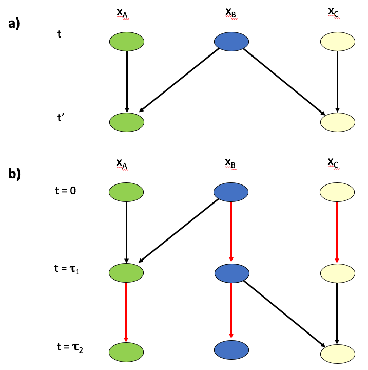
Figure 1: a) The upper figure illustrates the example BN discussed in the text. b) The lower figure illustrates that same BN, expanded into a sequence of two solitary processes. Red arrows indicate the identity map. In the first solitary process the evolving system is subsystems $A$ and $B$, while in the second one it is subsystems $C$ and $B$.

In general, for any BN $G$, there are many equivalent BNs that have the same conditional distributions at their nodes as $G$, but physically implement those distributions in a different time order from $G$. Moreover, for any $G$, there is always such an equivalent BN in which only one node’s conditional distribution is implemented at a time. (This is called a “topological order” of $G$ koller2009probabilistic .) An example is the BN in Fig. 1(b), which implements the same conditional distributions as the BN in Fig. 1(a), but in two successive time-intervals rather than one.

Since it simplifies the analysis, from now on I follow ito2013information by restricting attention to such BNs where only one node’s conditional distribution is implemented at a time. This means that the evolution of any node $v$ in the BN occurs in a solitary process, where the evolving system $A$ is the union of the subsystem corresponding to $v$ and the subsystems corresponding to the parents of $v$. (See Appendix B in the Supplemental Material at [URL will be inserted by publisher] for a discussion of the thermodynamics when “two solitary processes run at the same time”.)) As an example, in Fig. 1(b), the update of subsystem $C$ in the time-interval $[\tau_{1},\tau_{2}]$ is a solitary process where the evolving system’s state is $(x_{B},x_{C})$, while the state of the fixed system is $x_{A}$. (Note from Eq. 5 that we cannot identify $C$ by itself as the solitary system, since the evolution of $x_{C}$ depends on $x_{B}$ as well as its own state, $x_{C}$.)

I write the set of nodes in a BN as $V$, and label them with successive integers. In general, more than one $v\in V$ might refer to evolution of the same subsystem, just at different times. In light of the fact that the evolving systems in the solitary processes will be unions of a node and its parents, for any $V^{\prime}\subset V$ I define $[V^{\prime}]:=V^{\prime}\cup\mathrm{pa}(V^{\prime}):=\cup_{v\in V^{\prime}}\;v\cup\mathrm{pa}(v)$, where $\mathrm{pa}(v)$ indicates the parents of node $v$. In addition, for any $V^{\prime}\subset V$, I define $-V^{\prime}:=V\setminus V^{\prime}$. I write the distribution over all subsystems after the process implementing node $v$ has run as $p^{{v}}$, and unless indicated otherwise, assume that it runs in the time interval $[v-1,v]$. The root nodes are jointly sampled at $t=0$ according to distribution $p^0(x)$, resulting in full trajectory ${\boldsymbol{x}}$. For any $v\in V$, I write the segment of ${\boldsymbol{x}}$ corresponding to the time interval when node $v$ runs as ${\boldsymbol{x}}^v$, reserving subscripts for specification of particular subsystems. As an example of this notation, ${\boldsymbol{x}}_{[v]}$ is the full trajectory of the components of ${\boldsymbol{x}}$ specified by $[v]$, i.e., ${\boldsymbol{x}}_{[v]}\;=\;{\boldsymbol{x}}_{\{v^{\prime}\in v\cup\mathrm{pa}(v)\}}$, while ${\boldsymbol{x}}^v_{[v]}$ is the segment of that trajectory in the time interval $[v-1,v]$.

Let $\pi=\{\pi_{v}(x_{v}|x_{\mathrm{pa}(v)})\}$ indicate the set of the conditional distributions at the nodes of the BN. I write the local EP generated in the associated solitary process as $\sigma_{[v]}$. Since EP is cumulative over time, by repeated application of Eq. 3, once for each node in the BN, we see that the global EP incurred by running all nodes in the BN if the joint system follows trajectory ${\boldsymbol{x}}$ is

$$\sigma({\boldsymbol{x}},\pi,p^{0}) =\sum_{v=1}^{|V|}\bigg{[}{\sigma}_{[v]}({\boldsymbol{x}}_{[v]}^v,\pi_{v},p^{{v-1}})$$

$$\qquad\qquad+\left(I_{p^{{v-1}}}\big{(}{\boldsymbol{x}}_{[v]}^v;{\boldsymbol{x}}_{-[v]}^v\big{)}-I_{p^{{v}}}\big{(}{\boldsymbol{x}}_{[v]}^v;{\boldsymbol{x}}_{-[v]}^v\big{)}\right)\bigg{]}$$

$$:=\sum_{v\in V}{\sigma}_{[v]}({\boldsymbol{x}}^v)-\Delta I^v({\boldsymbol{x}})$$ (7)

(Note that the superscript $v$ on $\Delta I^v({\boldsymbol{x}})$ indicates both the time interval and the evolving system.)

The expectation of the local EP generated by each solitary process must be non-negative. (This is not true for the analogous expected EP considered in ito2013information ; see Appendix C in the Supplemental Material at [URL will be inserted by publisher].) So Eq. 7 means that $-\left\langle\sum_{v\in V}\Delta I^v({\boldsymbol{x}})\right\rangle$ is a lower bound on the expected global EP. In addition, the sum in Eq. 7 is independent of the topological order of the nodes in the BN, so long as each conditional distribution $\pi_{v}$ is fixed as we vary that order. (See Appendix D in the Supplemental Material at [URL will be inserted by publisher].) So $-\left\langle\sum_{v\in V}\Delta I^v({\boldsymbol{x}})\right\rangle$ is the same lower bound on the EP no matter what topological order we use.

FT’s and TUR’s for Bayesian networks.— My first result is an FT relating the local EPs when each node runs with the associated changes in mutual information between the states of the evolving and fixed systems:

$$\left\langle\exp\sum_{v\in V}\left(\Delta I^v-{\sigma}_{[v]}\right)\right\rangle=1$$ (8)

where the expectation is over all trajectories. (See Appendix E in the Supplemental Material at [URL will be inserted by publisher] for proofs of the FTs presented in this section, along with some intermediate results.) Eq. 8 means that the larger the sum of the drops in mutual information when the nodes run, the larger must be the sum of EPs generated by running those nodes.

In addition, for every node $v\in V$, and for all associated joint values $({\sigma}_{[v]},\Delta I^v)$ that occur with nonzero probability, there is a “conditional FT”:

$$\left\langle\exp\sum_{v^{\prime}\neq v}\left(\Delta I^{v^{\prime}}-{\sigma}_{[v^{\prime}]}\right)\right\rangle_{{{\mathbb{P}}}(.|{\sigma}_{[v]},\Delta I^v)} =1$$ (9)

where the subscript indicates that the expectation is conditional on the given pair of values, $({\sigma}_{[v]},\Delta I^v)$.

Concretely, Eq. 9 concerns the case where we are able to measure the EP generated by the evolving system $[v]$ when node $v$ runs, together with the associated change in mutual information between the state of the evolving and fixed systems. It says that if we average over all instances where that EP and mutual information drop have those known values, then the associated (exponential of the sum of the) EPs and drops of mutual information when all the other nodes besides $v$ are run must average to $1$.

${\sigma}_{[v]}$ obeys the usual FT when considered by itself, in isolation from the rest of the subsystems. This means that there is a second set of conditional FTs, which apply if the experimentalist can only observe the local EP ${\sigma}_{[v]}$:

$$\left\langle\exp\left(\Delta I^v+\sum_{v^{\prime}\neq v}\left(\Delta I^{v^{\prime}}-{\sigma}_{[v^{\prime}]}\right)\right)\right\rangle_{{{\mathbb{P}}}(.|{\sigma}_{[v]})} =1$$ (10)

Eqs. 8, 9 and 10 generalize to FTs that concern sums over arbitrary subsets of $V$ rather than all of $V$, and / or arbitrary subsets of all the subsystems. Also, Eqs. 9 and 10 generalize to probability distributions conditioned on simultaneous properties of multiple nodes $v$, not just one.

Each ${\sigma}_{[v]}$ bounds currents generated in the associated evolving system $[v]$, in accordance with the usual TURs. (This is not true for the analogous expected EP considered in ito2013information .) We can exploit this to derive TURs which relate the global EP generated by running an entire BN to the currents in each evolving system when it runs. (See Appendix E in the Supplemental Material at [URL will be inserted by publisher] for a quick review of TUR terminology and proofs of the TURs derived here.)

As an illustration, slightly generalize our scenario so that the solitary process running each node $v$ takes a total time $\tau_{v}$ to run, and therefore starts to run at time $t_{v-1}=\sum_{v^{\prime}\leq v-1}\tau_{v^{\prime}}$. Let $j_{[v]}^t({\boldsymbol{x}})$ be any instantaneous current over $X_{[v]}$ at time $t$. Write the time-integrated current over the associated time interval as $J_{[v]}({\boldsymbol{x}})=\int_{t_{v-1}}^{t_{v}}dtj_{[v]}^t({\boldsymbol{x}})$. Assume that the rate matrix of the full system is constant throughout each of the intervals when a node runs (although it will change from one such interval to another, in general). Then we can exploit a recently derived TUR liu2019thermodynamic to establish that the expected global EP bounds the precisions of the currents in the subsystems along with the associated drops in mutual information:

$$\left\langle\sigma\right\rangle \geq\sum_{v}\left(\dfrac{2\tau_{v}^2\left\langle j_{[v]}^{t_{v}}\right\rangle^2}{{\mbox{Var}}(J_{[v]})}-\left\langle\Delta I^v\right\rangle\right)$$ (11)

This TUR holds without any restrictions on the distributions at the start or end of the interval when any specific node $v$ runs. However, suppose that for each node $v$, $p^v=p^{v-1}$, and so in particular the evolving system’s distribution is the same at the start and end of the interval when it evolves. Also allow the rate matrix when node $v$ runs to vary rather than stay constant, so long as it is symmetric about the time $[t^{v-1},t^v]\,/\,2$. In this situation we can exploit the generalized TUR hasegawa2019generalized ; falasco2019unifying to establish a different TUR for the full BN:

$$\left\langle\sigma\right\rangle \geq\sum_{v}\left(\ln\bigg{[}\dfrac{2\langle J_{[v]}\rangle^2}{{\mbox{Var}}(J_{[v]})}+1\bigg{]}-\left\langle\Delta I^v\right\rangle\right)$$ (12)

Now suppose that in fact every evolving system $[v]$ is in an NESS when node $v$ runs (though the NESS’s may differ depending on which node is running). Then

$$\left\langle\sigma\right\rangle \geq\sum_{v}\left(\dfrac{2\langle J_{[v]}\rangle^2}{{\mbox{Var}}(J_{[v]})}-\left\langle\Delta I^v\right\rangle\right)$$ (13)

This formula holds even if the distribution of the global system is continually changing, so long as during each solitary process the marginal distribution of the associated solitary system does not change.

Example of TUR’s for a BN.— Suppose we have three subsystems, $A,B$ and $C$, jointly evolving as in Fig. 1(b). So in the first solitary process the evolving system is the composite system $AB$ and $C$ is the fixed system, while in the second solitary process the evolving system is the composite system $BC$ and $A$ is the fixed system. Let $J_{A}(.)$ be any net current among subsystem $A$’s states during the first solitary process, and similarly for $J_{C}(.)$, with $j_{A}^t(.)$ and $j_{C}^t(.)$ the associated instantaneous currents at time $t$. Assume that the rate matrix implementing the first solitary process is constant during that process, and similarly for the (different) rate matrix implementing the second solitary process. So in the first solitary process subsystem $A$ evolves according to a matrix exponential, where the precise matrix being exponentiated is specified by (the unchanging) value of $x_{B}$, i.e.,

$$P(x_{A}^{\tau_{1}}\,|\,x_{A}^0,x^0_{B}) =\exp{\left(\tau_{1}W^{x_{B}^0}_{A}\right)}\bigg{|}_{x_{A}^{\tau_{1}},x_{A}^{0}}$$ (14)

and similarly for subsystem $C$.

Plugging into Eq. 11 and then using the fact that $x_{B}$ never changes in either solitary process,

$$\left\langle\sigma\right\rangle \geq\dfrac{2\tau_{1}^2\langle j_{A}^{\tau_{1}}\rangle^2}{{\mbox{Var}}(J_{A})}+\dfrac{2\tau_{2}^2\langle j_{C}^{\tau_{1}+\tau_{2}}\rangle^2}{{\mbox{Var}}(J_{C})}-\left\langle\Delta I^A\right\rangle-\left\langle\Delta I^C\right\rangle$$ (15)

$$=\dfrac{2\tau_{1}^2\langle j_{A}^{\tau_{1}}\rangle^2}{{\mbox{Var}}(J_{A})}+\dfrac{2\tau_{2}^2\langle j_{C}^{\tau_{1}+\tau_{2}}\rangle^2}{{\mbox{Var}}(J_{C})}$$

$$\;\;\;\;+\Delta S(X_{A},X_{B},X_{C})-\Delta S(X_{A},X_{B})-\Delta S(X_{C},X_{B})$$ (16)

where here $\Delta$ indicates the value of a quantity at $t=\tau_{1}+\tau_{2}$ minus its value at $t=0$. Eq. 16 provides a trade-off among global EP, three entropy drops (from the beginning to the end of the full BN), the instantaneous currents at the moments when each of the two subsystems finishes its update, and associated variances of net currents. Note that the RHS of Eq. 16 would not change if the two solitary processes had been run in the reverse order.

Now consider the case where $X_{B}$ is binary, both matrices $W^{x_{B}}_{A}$ have a (unique) NESS over $X_{A}$, but that NESS differs for the two $x_{B}$ values. Suppose further that the initial distribution is

$$p^0(x_{A},x_{B},x_{C}) =p^0(x_{B})p^0(x_{A}|x_{B})\delta(x_{C},x_{A})$$ (17)

Next, assume that for both values of $x_{B}$, $p^0(x_{A}|x_{B})$ is the NESS of the associated rate matrix $W^{x_{B}}_{A}$. This guarantees that $p^0(x_{A},x_{B})$ is a NESS during the first solitary process, regardless of $p^0(x_{B})$. For completeness, assume that the second solitary process proceeds the same way, just with subsystem $C$ substituted for subsystem $A$. Therefore we can apply Eq. 13.

Since there are nonzero probability currents in an NESS, there is nonzero probability that the ending state of $x_{A}$ after the first solitary process runs differs from the state of $x_{C}$ then. However, with probability $1$ their initial states were identical. So there is a drop in (expected) mutual information between the evolving and fixed systems of the first solitary process. The same is true for the second solitary process. These two drops in mutual information mean that the global system is not in an NESS throughout the full process. In addition, they provide positive values to two terms on the RHS of Eq. 13, thereby setting a floor for a tradeoff between global EP and the precisions of the two solitary processes.

Discussion.— In this paper I derive new FTs and TURs for systems composed of multiple interacting subsystems. Following ito2013information , I formulate the interactions of those subsystems as a Bayesian network. However, in contrast to ito2013information , I identify the evolving systems when each node in the BN is implemented in a way that ensures that the associated EP has the conventional thermodynamic properties of EP (e.g., that its expectation is non-negative). This is crucial to the derivation of the FTs and TURs. It also allows me to derive conditional FTs, involving probabilities of global EP conditioned on a given EP value of one of the subsystems.

I would like to thank Kangqiao Liu, Jan Korbel and Artemy Kolchinsky for helpful discussion. This work was supported by the Santa Fe Institute, Grant No. CHE-1648973 from the US National Science Foundation and Grant No. FQXi-RFP-IPW-1912 from the FQXi foundation. The opinions expressed in this paper are those of the author and do not necessarily reflect the view of the National Science Foundation.

Appendix A Technical details of the extension of Bayes nets considered in this paper.

Recall from the main text that we have a physical system comprising a finite set $\mathcal{S}$ of subsystems, with joint states $x=(x_{1},x_{2},\ldots,x_{|\mathcal{S}|}\in X$. We also have a separate BN with a set of nodes $\mathcal{V}$. I indicate the root nodes of the BN as $R\subset\mathcal{V}$, and write the non-root nodes as $V:=\mathcal{V}\setminus R$. (See koller2009probabilistic ; neapolitan2004learning for formal definitions of BNs and the associated terminology.)

To connect the BN with $\mathcal{S}$, we need a function $g:\mathcal{V}\rightarrow\mathcal{S}$ that maps each $v\in\mathcal{V}$ to one of the subsystems. Note that in general $g$ will not be invertible; the same subsystem may change its state in a conditional distribution specified by more than one node of the BN. (In the main text, following the convention in ito2013information , $g$ is implicit.)

Write the initial distribution of the joint state of the subsystems in terms of the distribution over the root nodes of the BN, as $p^0(x_{g(R)})$. So the distribution over $x_{g(v)}$ after any non-root node $v$ runs is

$$\!\!\!\!\!\!\!\!\sum_{x_{g(R)}}p^0(x_{g(R)})\;\bigg{[}\bigg{(}\sum_{x_{g(\mathrm{Anc}[v])}}\prod_{v^{\prime}\in\mathrm{Anc}[v]}\pi_{v^{\prime}}(x_{g(v^{\prime})}|x_{g(\mathrm{pa}(v^{\prime}))})\bigg{)}$$

$$\qquad\qquad\qquad\qquad\qquad\qquad\;\;\;\;\times\pi_{v}(x_{g(v)}|x_{g(\mathrm{pa}(v))})\bigg{]}$$ (18)

where $Anc[v]$ is the set of ancestor nodes of $v$ that are not root nodes. Below I will often write $x_{v}$ as shorthand for $x_{g(v)}$.

As described in the text, I follow ito2013information and assume that the conditional distributions of the BN’s nodes are implemented one after another, in a sequence of solitary processes specified by a topological order of the BN. I index the nodes by their (integer-valued) position in the topological order, with an index $v\in\{1-|R|,\ldots,|V|\}$, so that the non-root nodes start with $v>0$.

As an aside, note that one cannot model the dynamics when node $v$ runs as a solitary process where the subsystem $v$ considered by itself is the evolving system. The reason is that since the dynamics of $x_{g(v)}$ depends on the value of $x_{g(\mathrm{pa}(v))}$ when $v$ runs, Eq. 4 does not hold for any function ${{\mathcal{Q}}}_{1}$ if ${\boldsymbol{x}}_{A}$ is set to $x_{g(v)}$.

For this framework to give both a complete and consistent representation of the thermodynamics of a set of evolving subsystems, several requirements must be met. First, there must be exactly one root node $r$ corresponds to each subsystem, i.e., for all subsystems $i$, $g(r)=i$ for exactly one $r\in R$. Second, the joint distribution $p^0(x_{g(R)})$ must have been sampled before any non-root node $v$ runs. (This ensures that every subsystem has a well-defined state by the time any non-root node $v$ runs.)

A third, more subtle requirement, reflects the fact that we want every non-root node in the DAG to represent a change in the state of one of the physical systems. This means that for each root node $r$, corresponding to subsystem $i=g(r)$, all other nodes $v^{\prime}\in g^{-1}(i)$ representing states of that subsystem lie on a single path of connected edges leading out of $r$. This then implies that for all non-root nodes $v$, there is one (and only one) parent of $v$ in the DAG, $v^{\prime}$, such that $g(v^{\prime})=g(v)$; we interpret the value of $x_{g(v^{\prime})}$ when node $v$ starts to run as the initial state of $X_{g(v)}$ at the beginning of a process updating it, while the value of $x_{g(v)}$ when node $v$ has finished running is the state of $X_{g(v)}$ when that update has completed.

Finally, I require that we can implement the BN in a specific type of topological order: one where no subsystem’s update at a node $v$ depends on an old state of another subsystem which has been overwritten by the time that $v$ is executed. Formally, this requirement means that for all nodes $v$, there is no $v^{\prime}\in\mathrm{pa}(v)$ and other node $v^{\prime\prime}$ such that: $g(v^{\prime})=g(v^{\prime\prime})$, $v^{\prime}$ is an ancestor of $v^{\prime\prime}$, and $v^{\prime\prime}$ occurs before $v$ in the topological order. This ensures that the physical process implementing the BN is Markovian.

Note that not all BNs can be represented in a topological order that respects this last requirement. Most simply, suppose we have two subsystems, $X$ and $Y$, with states $x$ and $y$. Suppose that under the BN governing their joint dynamics, $x^1$ depends on both $x^0$ and $y^0$, and $y^1$ also depends on both $x^0$ and $y^0$. So if we update $X$ first under the topological order, then no physical process can properly update $Y$ in a subsequent process by coupling to the state of $X$, since $x^0$ no longer describes the state of $X$. Similarly, if we update $Y$ first, then no physical process can properly update $X$ after that by coupling to the state of $Y$ since $y^0$ no longer describes the state of $Y$. So this requirement is actually a restriction on the BNs being considered in this paper.

These requirements are all assumed in ito2013information , implicitly or otherwise. In particular, to see that the analysis in ito2013information also assumes that the physical process updating the state of the subsystem $g(v)$ can be treated as a solitary process, where the evolving system is $A=g(v)\cup g(pa(v))$, note that in Eq. 4 of ito2013information , the two conditional probabilities on the RHS are conditioned only on ${\mathcal{B}}^{k+1}$. So it is being assumed that the entropy flow into the baths can be written as a function of the state of the physical variable $x$ at the times $k$ and $k+1$, as well as the (identical) states of the variables corresponding to its parents at those two times, i.e., that condition 2 of a solitary process is being obeyed.

However, for simplicity I modify the formulation in ito2013information by allowing the subsystems to have their initial states set in parallel, by sampling the joint distribution $p^0$ over the root nodes at once, rather than require that those nodes be sampled independently, one after the other. In addition, for convenience I relax the standard BN requirement that the distribution over the root nodes be a product distribution, whereas ito2013information does not address this issue. Ultimately, allowing the root nodes to be jointly sampled is just a modeling choice. An alternative, adhering to the conventional BN requirement that all root nodes be sampled independently, would be to modify the DA to include a single extra node that is a shared parent of what (in the framework here) is the set $R$ of root nodes.

The framework defined above is similar to several graphical models in the literature, including non-stationary dynamic Bayesian networks robinson2009non , time-varying dynamic Bayesian networks song2009time , and non-homogeneous dynamic Bayesian networks dondelinger2013non , among others. Nonetheless, for simplicity, I will simply refer to this structure as a Bayes net, even though that is not exactly accurate.

Finally, as a technical comment, it is important to note that there are an infinite set of discrete-time conditional distributions $\pi_{v}(x_{v}^{v+1}|x_{v}^{v})$ that cannot be implemented using a CTMC over $X_{g([v])}$. Instead, in order to use a CTMC to model the dynamical process that results in that conditional distribution, there must be a set of extra “hidden” states of subsystem $g(v)$, in addition to the “visible” states in $X_{g(v)}$, and the CTMC must couple those two sets of states when it runs that conditional distribution to update that subsystem owen_number_2018 ; wolpert_spacetime_2019 .

However, at both $t=v-1$ and $t=v$, the beginning and end of when node $v$ runs, the state of subsystem $g(v)$ must be visible, i.e., it must lie in $X_{g(v)}$ at those two times. (If that weren’t the case, then we could not be sure that the discrete time dynamics is actually given by $\pi_{v}(x_{v}^{v+1}|x_{v}^{v})$ operating on $p^v(x^v_{\mathrm{pa}(v)})$.) Accordingly, any hidden states can be ignored in calculating the drop in mutual information as node $v$ runs. For the same reason, the change in $\ln[p^t({\boldsymbol{x}})]$ from $t=v$ to $t=v+1$ doesn’t depend on whether hidden states exist. So the only effect of such states on Eq. (5) of the main text is to modify the EF function of the process updating node $v$, ${{\mathcal{Q}}}_{v}(.,.)$ (and similarly for Eq. (1) of the main text.) Therefore their only effect on Eq. (7) in the main text — which is the starting point for the results in this paper concerning solitary process formulations of BNs — is to change the EF function implicitly defining ${\sigma}_{[A]}(.,.)$. Since the detailed form of the EF function is irrelevant for the results in this paper in the way that they are stated (the EF function for updating node $v$ is subsumed in the function ${\sigma}_{[v]}(.,.)$), we can ignore hidden states for the purposes of this paper.

Appendix B Path-wise subsystem processes

In the text, for simplicity, I considered the case where each subsystem updates its state in a solitary process, during which no other subsystem changes its state. However it is straightforward to weaken that restriction, to allow multiple subsystems to change their state at the same time, so long as they are independent of one another during that simultaneous update. While this flexibility is not exploited in the main text, it is worth describing its thermodynamic properties. I do that in this appendix.

To begin, write the multi-information of a joint distribution over a set of random variables, $p(X_{1},X_{2},...)$, as

$${\mathcal{I}}(p) :=\left[\sum_{i}S(p(X_{i}))\right]-S(p(X))$$ (19)

(Multi-information is also sometimes called “total correlation” in the literature.) Mutual information is the special case of multi-information where there are exactly two random variables. I will use “path” and “trajectory” interchangeably, to mean a function from time into a state space. In the usual way, I use the argument list of a probability distribution to indicate what random variables have been marginalized, e.g., $P(x)=\sum_{y}p(x,y)$.

Consider a CTMC governing evolution during time interval $[t_{0},t_{1}]$. That CTMC is a (path-wise) subsystem process if

1. The subsystems evolve independently of one another, i.e., the discrete-time conditional distribution over the joint state space is

   $$\pi({\boldsymbol{x}}^{t_{1}}|{\boldsymbol{x}}^{t_{0}})=\prod_{i\in\mathcal{S}}\pi_{i}({\boldsymbol{x}}_{i}^{t_{1}}|{\boldsymbol{x}}_{i}^{t_{0}})$$ (20)

2. There are $|\mathcal{S}|$ functions, ${{\mathcal{Q}}}_{i}(.)$, such that the entropy flow (EF) into the joint system during the process if the full system follows trajectory ${\boldsymbol{x}}$ can be written as

   $${{\mathcal{Q}}}({\boldsymbol{x}})=\sum_{i\in\mathcal{S}}{{\mathcal{Q}}}_{i}({\boldsymbol{x}}_{i})$$ (21)

   for all trajectories ${\boldsymbol{x}}$ that have nonzero probability under the protocol for initial distribution $p^{t_{0}}$. (Recall that the entire sequence of Hamiltonians and rate matrices is referred to as a “protocol” in stochastic thermodynamics.)

Intuitively, in a subsystem process the separate subsystems evolve in complete isolation from one another, with decoupled Hamiltonians and rate matrices. (See wolpert2020thermodynamics ; wolpert_thermo_comp_review_2019 for explicit examples of CTMCs that implement subsystem processes, for the special case where there are two subsystems.)

I use the term (path-wise, subsystem) Landauer loss to refer to the extra, unavoidable EP generated by implementing the protocol due to the fact that we do so with a subsystem process:

$${\mathcal{L}}({\boldsymbol{x}},p) :=\sigma({\boldsymbol{x}},p)-\sum_{i=1}^N{\sigma}_{i}({\boldsymbol{x}}_{i},p_{i})$$

$$={\mathcal{I}}_{p^{t_{0}}}({\boldsymbol{x}}^{t_{0}})-{\mathcal{I}}_{p^{t_{1}}}({\boldsymbol{x}}^{t_{1}})$$

$$:=-\Delta{\mathcal{I}}_{p}({\boldsymbol{x}})$$ (22)

where the second line uses condition (2) of path-wise subsystem processes to cancel the EFs. (The reason for the name is that the “Landauer cost” of implementing $\pi({\boldsymbol{x}}^{t_{1}}|{\boldsymbol{x}}^{t_{0}})$ — the minimal EF needed by any physical process that implements that conditional distribution — is increased by ${\mathcal{L}}({\boldsymbol{x}},p)$ if we add the requirement that the process obey condition (2) of path-wise subsystem processes.) Note that even though $\Delta{\mathcal{I}}_{p}(.)$ is written as a function of an entire trajectory, its value only depends and the initial and final states of the trajectory.

Both (expected) subsystem EP and global EP are always non-negative. Moreover, by Eq. 22, if the expected multi-information among the subsystems decreases in a subsystem process, the Landauer loss must be strictly positive — and so the global EP has a strictly positive lower bound. This is true no matter how thermodynamically efficiently the individual subsystems evolve.

One way to understand this phenomenon is to note that in general the Shannon information stored in the initial statistical coupling among the subsystems will diminish (and maybe disappear entirely) as the process runs. However, for each subsystem $i$ the rate matrix governing how $x_{i}$ evolves cannot depend on the states of the rest of the subsystems, $x_{-i}$, due to condition (2) of subsystem processes. So that rate matrix cannot exploit the information in the statistical coupling between the initial states of the subsystems to reduce the total amount of entropy that is produced as the information about the initial coupling of the subsystem states disappears. In contrast, if it were not for condition (2), then the rate matrix governing the dynamics of $x_{i}$ could depend on the value of $x_{-i}$, and therefore could exploit that value to reduce the amount of entropy that is produced as the information about the initial coupling of the subsystem states disappears. (See wolpert2020thermodynamics ; wolpert_thermo_comp_review_2019 .)

These results do not require that the underlying process generating trajectories is a CTMC. However, from now on I assume that in fact the dynamics is generated by a CTMC, so that the conventional fluctuation theorems and uncertainty relations all hold.

Appendix C The differences between the thermodynamic properties of ${\sigma}_{[A]}$ and ${\sigma}_{A}$.

When $v$ runs, the set of subsystems $[v]=g(v)\cup g(\mathrm{pa}(v))$ form a solitary system, while the subsystem $g(v)$ is only an evolving system. This is why I write the local EP generated by $[v]$ when node $v$ runs as ${\sigma}_{[v]}({\boldsymbol{x}})$ for short. In general, this local EP generated by the set of subsystems $[v]$ when $g(v)$ runs will differ from the local EP generated by just $g(v)$ when node $v$ runs; they are related by

$${\sigma}_{v}({\boldsymbol{x}}) ={\sigma}_{[v]}({\boldsymbol{x}})+\Delta^v\ln\left[{p({\boldsymbol{x}}_{\mathrm{pa}(v)}\,|\,{\boldsymbol{x}}_{v})}\right]$$ (23)

where $\Delta^vf[p({\boldsymbol{x}})]$ is shorthand for $f[p^v({\boldsymbol{x}})]-f[p^{v-1}({\boldsymbol{x}})]$. (See Eqs. 2 and 4.) As described above, the analysis in ito2013information concerns $\sigma_{v}$ rather than $\sigma_{[v]}$.

The expected value of ${\sigma}_{v}$ can be negative, in contrast to the expected value of ${\sigma}_{[v]}$. In addition, while the usual FTs and TURs apply to the EP ${\sigma}_{[v]}$, they do not apply to ${\sigma}_{v}$ in general. This is why I formulate the results in the text in terms of ${\sigma}_{[v]}$. However, if desired these results can be recast in terms of ${\sigma}_{v}$, by using Eq. 23. This allows the results of this paper to be connected with those in ito2013information .

In the rest of this appendix I discuss this relationship between the two kinds of EP in more detail. The first thing to note is that there are several specific thermodynamic properties of the EP of the evolving system ${\sigma}_{[A]}$ in a solitary process that need not hold for the EP of the evolving system ${\sigma}_{A}$ in a general semi-fixed process. Perhaps the most important is that in keeping with the conventional second law, in a solitary process the expected subsystem EP of the evolving system is non-negative. i.e., $\langle{\sigma}_{A}\rangle\geq 0$, whereas $\langle{\sigma}_{A}\rangle$ can be strictly negative. As an explicit demonstration of such a case where the expected EP can be negative, suppose that the entire joint system evolves in a thermodynamically reversible process, so that $\langle\sigma\rangle=0$. Then ${{\mathcal{Q}}}({\boldsymbol{x}},p^{t_{0}})=\ln[p^{t_{0}}({\boldsymbol{x}})]-\ln[p^{t_{1}}({\boldsymbol{x}})]$. Therefore

$$\langle{\sigma}_{A}\rangle =S_{{t_{1}}}(X_{A})-S_{{t_{0}}}(X_{A})-\left[S_{{t_{1}}}(X_{A},X_{B})-S_{{t_{0}}}(X_{A},X_{B})\right]$$

$$=S_{{t_{0}}}(X_{A}|X_{B})-S_{{t_{1}}}(X_{A}|X_{B})$$ (24)

A priori, this drop in the conditional entropy of the evolving system’s state given the fixed system’s state can be positive or negative.

A second important difference arises if we consider the minimal amount of work required to send the ending joint distribution of a semi-fixed process, $p_{f}$, back to the initial one, $p_{i}$. The difference between the amount of work expended in getting from $p_{i}$ to $p_{f}$ in the first place and this minimal amount of work to go back is sometimes called the “dissipated” work in going from $p_{i}$ to $p_{f}$, because it is the minimal amount of work lost to the heat bath if one were to run a full cycle $p_{i}\rightarrow p_{f}\rightarrow p_{i}$. Much of the stochastic thermodynamics literature presumes that dissipated work can be treated as a synonym for EP. In agreement with this, the dissipated work in a solitary process always equals the expected subsystem EP, $\langle{\sigma}_{[A]}\rangle$. In contrast, dissipated work does not equal $\langle\overline{\sigma}_{i}\rangle$ in semi-fixed processes, in general.

Another difference is that in a solitary process the conventional FT holds for the evolving system with state space $X_{A}$, considered in isolation from the fixed system, if the EP in that FT is identified as ${\sigma}_{[A]}({\boldsymbol{x}}_{1},p_{1})$. However, in general the conventional FT will not hold in general for a semi-fixed process with state space $X_{A}$ in an arbitrary semi-fixed process, if the EP in that FT is identified as ${\sigma}_{A}({\boldsymbol{x}},p)$.

As a final example, the expected EP of the evolving system in a solitary process bounds the precision of any current defined over the state of the subsystem, in the usual way given by the thermodynamic uncertainty relations falasco2019unifying . However, the expected EP of the evolving system in a semi-fixed process need not have so simple a relationship with the current in that subsystem.

Example 1.

Consider a process involving three subsystems, $A$, $B$ and $C$. Only subsystem $A$ changes its state in this process, and the dynamics of subsystem $A$ depends on the state of subsystem $B$, but not on the state of subsystem $C$. We can formulate this process as a semi-fixed process where either subsystem $A$ or the joint subsystem $AB$ is the evolving system.

Note though that we cannot identify subsystem $A$ as the evolving system of a solitary process, with the joint subsystem $BC$ being the fixed subsystem. (Since the evolution of subsystem $A$ depends on the state of subsystem $B$, condition (1) would be violated.)

On the other hand, the situation is not so clear-cut if we ask whether the process is a solitary process with $AB$ the evolving system. If the joint subsystem $AB$ is physically decoupled from subsystem $C$, with no interaction Hamiltonian coupling $C$ to the other subsystems, and no coupling of $C$ with $AB$ in the rate matrix for the full system $ABC$, then we have a solitary process, with the evolving system identified as the joint subsystem $AB$. However, as an alternative, we could run the entire process in a way that is globally thermodynamically reversible, incurring zero global EP. (N.b., in general this would require an interaction Hamiltonian coupling $C$ to the other subsystems, and require that the rate matrix for the full system $ABC$ couples the dynamics of $C$ to that of $AB$.) In this case, the bound in Eq. 3 would be violated in general if we identify $AB$ as the evolving system (e.g., if the expected drop in mutual information is strictly nonzero). So the overall process would not a solitary process with $AB$ the evolving system.

This demonstrates that in general, just specifying the joint dynamics of a co-evolving set of subsystems does not determine whether we can view a particular physical process that implements that dynamics as a solitary process, for some appropriately identified evolving system.

Appendix D Global EP is independent of the topological order of the nodes in the BN

By hypothesis, for all $v\in V$, the physical process that implements the conditional distribution $\pi_{v}(x_{g(v)}|x_{g(\mathrm{pa}(v))})$ is the same in any two topological orders. So changing the topological order doesn’t change any of the values ${\sigma}_{[v]}$. Therefore to establish the claim, we need to establish that $-\sum_{v\in V}\Delta I^v({\boldsymbol{x}})$ is independent of the topological order.

To do that, given a topological order, label the nodes $v\in V$ in the sequence they occur in that topological order as $1,2,\ldots|V|$, so that they occur in corresponding time intervals $[0,1],[1,2],\ldots,[|V|-1,|V|]$. (Note that in general it may be that more than one of those nodes change the state of the same subsystem.) Express $g(.)$ accordingly. Next, use the fact that while the marginal entropy of the evolving system changes during a solitary process, the marginal entropy of the semi-fixed system doesn’t change, to expand

$$-\sum_{v\in V}\Delta I^v({\boldsymbol{x}})\;=\; -\left[\left(\ln(p^0_{g(1)}({\boldsymbol{x}}))+\ln(p^0_{-g(1)}({\boldsymbol{x}}))-\ln(p^0({\boldsymbol{x}}))\right)-\left(\ln(p^1_{g(1)}({\boldsymbol{x}}))+\ln(p^0_{-g(1)}({\boldsymbol{x}}))-\ln(p^1({\boldsymbol{x}})\right)\right]$$

$$\qquad-\left[\left(\ln(p^1_{g(2)}({\boldsymbol{x}}))+\ln(p^1_{-g(2)}({\boldsymbol{x}}))-\ln(p^1({\boldsymbol{x}}))\right)-\left(\ln(p^2_{g(2)}({\boldsymbol{x}}))+\ln(p^1_{-g(2)}({\boldsymbol{x}}))-\ln(p^2({\boldsymbol{x}}))\right)\right]$$

$$\qquad-\ldots$$

$$\qquad-\left[\left(\ln(p^{|V|-1}_{g(|V|)}({\boldsymbol{x}}))+\ln(p^{|V|-1}_{-g(|V|)}({\boldsymbol{x}}))-\ln(p^{|V|-1}({\boldsymbol{x}}))\right)-\left(\ln(p^{|V|}_{g(|V|)}({\boldsymbol{x}}))+\ln(p^{|V|-1}_{-g(|V|)}({\boldsymbol{x}}))-\ln(p^{|V|}({\boldsymbol{x}}))\right)\right]$$

$$\;=\; \ln(p^0({\boldsymbol{x}}))-\ln(p^{|V|}({\boldsymbol{x}}))-\sum_{v}\ln(p^{v-1}_{g(v)}({\boldsymbol{x}}))-\ln(p^{v}_{g(v)}({\boldsymbol{x}}))$$

$$\;=\; \ln(p^0({\boldsymbol{x}}))-\ln(p^{|V|}({\boldsymbol{x}}))-\sum_{i}\sum_{v\in g^{-1}(i)}\ln(p^{v-1}_{g(v)}({\boldsymbol{x}}))-\ln(p^{v}_{g(v)}({\boldsymbol{x}}))$$

$$\;=\; \ln(p^0({\boldsymbol{x}}))-\ln(p^{|V|}({\boldsymbol{x}}))-\sum_{i}\ln(p^{0}_{i}({\boldsymbol{x}}))-\ln(p^{|V|}_{i}({\boldsymbol{x}}))$$ (25)

where the sums in last two equations are over the set of subsystems, and for simplicity I assume that each subsystem $i$ occurs in at least one node, i.e., for all subsystems $i$, $g^{-1}(i)\neq\varnothing$.

The RHS of Eq. 25 is fully specified by the combination of the BN and the initial distribution. So it cannot depend on the topological order. This establishes the claim.

As an aside, note that the expected value of the RHS of Eq. 25 can be written as the drop from the beginning to the end of the BN in the multi-information) among all the subsystems,

$$\left[\sum_{i}S(p_{i})\right]-S(p)$$ (26)

(See Eq. 19.) So loosely speaking, Eq. 25 says that the minimal expected global EP is the drop in “how much information the subsystems jointly provide about one another” from the beginning to the end of the full BN.

Appendix E Derivations of fluctuation theorems for Bayesian networks

Let $\tilde{{\boldsymbol{x}}}$ indicate the time-reversal of the trajectory ${\boldsymbol{x}}$. (For simplicity, I restrict attention to spaces $X_{i}$ whose elements are invariant under time-reversal.) Let ${\mathbb{P}}({\boldsymbol{x}})$ indicate the probability (density) of ${\boldsymbol{x}}$ under the forward protocol running the entire BN. Let $\tilde{{\mathbb{P}}}({\boldsymbol{x}})$ indicate the probability of the same trajectory if we run the protocol in time-reversed order, where the ending distribution over $X$ under ${\mathbb{P}}$ is the same as the starting distribution under $\tilde{{\mathbb{P}}}$. Also write $\tilde{{\boldsymbol{x}}}^v$ to indicate the time-reversal of the trajectory segment ${\boldsymbol{x}}^v$.

In the next subsection, I derive fluctuation theorems concerning probabilities of trajectories, and in the following subsection, I derive fluctuation theorems concerning the joint probability that each of the subsystem EPs has some associated specified value.

E.1 Fluctuation theorems for trajectories

Plugging Eq. (7) in the main text into the usual detailed fluctuation theorem (DFT) van2015ensemble gives the DFT,

$$\ln\bigg{[}\dfrac{{\mathbb{P}}({\boldsymbol{x}})}{\tilde{{\mathbb{P}}}(\tilde{{\boldsymbol{x}}})}\bigg{]} =\sum_{v=1}^{|V|}{\sigma}_{[v]}({\boldsymbol{x}}^v)-\Delta I^v({{\boldsymbol{x}}})$$ (27)

for all ${\boldsymbol{x}}$ with nonzero probability under ${\mathbb{P}}$. Exponentiating both sides of Eq. 27 and then integrating results in the integrated fluctuation theorem (IFT),

$$\left\langle e^{-\sum_{v=1}^{|V|}{\sigma}_{[v]}-\Delta I^v}\right\rangle :=\int d{\boldsymbol{x}}\,{\mathbb{P}}({\boldsymbol{x}})e^{\left(-\sum_{v=1}^{|V|}{\sigma}_{[v]}({\boldsymbol{x}}^v)-\Delta I^v({\boldsymbol{x}})\right)}$$

$$=1$$ (28)

In addition to applying to runs of the entire BN, the usual DFT applies separately to successive time intervals, i.e., to each successive interval at which exactly one node and its parents co-evolve as that node’s conditional distribution is executed. Therefore for all $v$,

$$\ln\bigg{[}\dfrac{{\mathbb{P}}({\boldsymbol{x}}^v)}{\tilde{{\mathbb{P}}}(\tilde{{\boldsymbol{x}}}^v)}\bigg{]} ={\sigma}_{[v]}({\boldsymbol{x}}^v)-\Delta I^v({\boldsymbol{x}})$$ (29)

which results in an IFT analogous to Eq. 28.

Combining Eqs. 27 and 29 gives

$${\mathcal{I}}({\mathbb{P}}({\boldsymbol{x}})) ={\mathcal{I}}(\tilde{\bm{P}}(\tilde{{\boldsymbol{x}}}))$$ (30)

where I define

$${\mathcal{I}}({\mathbb{P}}({\boldsymbol{x}})) :=\ln\left[\dfrac{{\mathbb{P}}({\boldsymbol{x}})}{\prod_{v=1}^{|V|}{\mathbb{P}}({\boldsymbol{x}}^v)}\right]$$ (31)

and similarly for ${\mathcal{I}}(\tilde{{\mathbb{P}}}(\tilde{{\boldsymbol{x}}}))$. Note that Eq. 35 can be rewritten as

$$\frac{{\mathbb{P}}\left({\boldsymbol{x}}\right)}{\tilde{{\mathbb{P}}}\left(\tilde{{\boldsymbol{x}}}\right)} =\prod_{v}\frac{{\mathbb{P}}\left({\boldsymbol{x}}^v\right)}{\tilde{{\mathbb{P}}}\left(\tilde{{\boldsymbol{x}}}^v\right)}$$ (32)

(This equality can also be derived directly, without invoking DFTs .)

The quantity ${\mathcal{I}}({\mathbb{P}}({\boldsymbol{x}}))$ defined in Eq. 31 is an extension of multi-information to concern probabilities of entire trajectories of the joint system. So loosely speaking, Eq. 35 means that the amount of information that the set of all the trajectory segments $\{{\boldsymbol{x}}^v\}$ provide about one another (under ${\mathbb{P}}$) equals the amount of information that the set of all the trajectory segments $\{\tilde{{\boldsymbol{x}}}^v\}$ provide about one another (under $\tilde{{\mathbb{P}}}$). (Note that the same subsystem may evolve in more than trajectory segment. ) In this sense, there is no arrow of time, as far as probabilities of trajectory segments are concerned.

We can also combine Eqs. 27 and 29 to derive DFTs and IFTs involving conditional probabilities, in which the trajectories of one or more of the subsystems are given. To illustrate this, pick any $V^{\prime}\subset V$, and use Eq. 29 to evaluate the terms on the RHS of Eq. 27 for all of the nodes $v\in V^{\prime}$. Define ${\boldsymbol{x}}^{V^{\prime}}:=\{{\boldsymbol{x}}^{v^{\prime}}:v^{\prime}\in V^{\prime}\}$, i.e., the “partial trajectory” given by all segments $v^{\prime}\in V^{\prime}$ of the trajectory ${\boldsymbol{x}}$. Then after clearing terms and using Eq. 32, we get the following conditional DFT, which must hold for all partial trajectories ${\boldsymbol{x}}^{V^{\prime}}$ with nonzero probability under ${\mathbb{P}}$:

$$\ln\left[\dfrac{{\mathbb{P}}\left({\boldsymbol{x}}|{\boldsymbol{x}}^{V^{\prime}}\right)}{\tilde{{\mathbb{P}}}\left(\tilde{{\boldsymbol{x}}}|\tilde{{\boldsymbol{x}}}^{V^{\prime}}\right)}\right] ={\mathcal{I}}(\tilde{{\mathbb{P}}}(\tilde{{\boldsymbol{x}}}^{V^{\prime}}))-{\mathcal{I}}({\mathbb{P}}({\boldsymbol{x}}^{V^{\prime}}))+\sum_{v\in V\setminus V^{\prime}}{\sigma}_{[v]}({\boldsymbol{x}}^v)-\Delta I^v({\boldsymbol{x}})$$ (33)

In turn, Eq. 33 gives the following conditional IFT which must hold for each partial trajectory ${\boldsymbol{x}}^{V^{\prime}}$ with nonzero probability under ${\mathbb{P}}$:

$$\left\langle e^{\left({\mathcal{I}}^{V^{\prime}}-\tilde{{\mathcal{I}}}^{V^{\prime}}+\sum_{v\in V\setminus V^{\prime}}\left(\Delta I_{v}-{\sigma}_{[v]}\right)\right)}\right\rangle_{{\mathbb{P}}(.|{\boldsymbol{x}}^{V^{\prime}})} =1$$ (34)

where ${\mathcal{I}}^{V^{\prime}}$ is shorthand for the random variable ${\mathcal{I}}({\mathbb{P}}({\boldsymbol{x}}^{V^{\prime}}))$ and similarly for $\tilde{{\mathcal{I}}}^{V^{\prime}}$. (Note that all terms in the exponent in Eq. 34 are defined in terms of the full joint distributions ${\mathbb{P}}({\boldsymbol{x}}))$, but that ${\boldsymbol{x}}$ is averaged according to ${\mathbb{P}}({\boldsymbol{x}}|{\boldsymbol{x}}^{V^{\prime}})$.)

Note that in addition to these results which hold when considering the entire system $X$, since each subsystem evolves in a solitary process, the usual DFT and IFT must hold for each subsystem $v$ considered in isolation, in the interval during which it runs. So for example,

$$\ln\bigg{[}\dfrac{{\mathbb{P}}\left({\boldsymbol{x}}^v_{[v]}\right)}{\tilde{{\mathbb{P}}}\left(\tilde{{\boldsymbol{x}}}^v_{[v]}\right)}\bigg{]} ={\sigma}_{[v]}({\boldsymbol{x}}^v)$$ (35)

(Compare to Eq. 29.) Eq. 35 gives us an additional set of conditional DFTs and IFTs. For example, it gives the following variant of Eq. 33

$$\ln\bigg{[}\dfrac{{\mathbb{P}}\left({\boldsymbol{x}}|{\boldsymbol{x}}^v_{[v]}\right)}{\tilde{{\mathbb{P}}}\left(\tilde{{\boldsymbol{x}}}|\tilde{{\boldsymbol{x}}}^v_{[v]}\right)}\bigg{]} =-\Delta I_{v}({\boldsymbol{x}})+\sum_{v^{\prime}\neq v}\left({\sigma}_{[v^{\prime}]}({\boldsymbol{x}}^{v^{\prime}})-\Delta I_{v^{\prime}}({\boldsymbol{x}})\right)$$ (36)

and the following variant of Eq. 34

$$\left\langle e^{-I_{v}+\sum_{v^{\prime}\neq v}\left(\Delta I_{v^{\prime}}-{\sigma}_{[v^{\prime}]}\right)}\right\rangle_{{\mathbb{P}}(.|{\boldsymbol{x}}^v_{[v]})} =1$$ (37)

Note that the numerator of the expression inside the logarithm on the LHS of Eq. 36 is a distribution conditioned on the joint trajectory of (the subsystem corresponding to) node $v$ and its parents when node $v$ runs. In contrast, the numerator inside the logarithm on the LHS of Eq. 33 is a distribution conditioned on the joint trajectory of all of the subsystems when node $v$ runs (not just the joint trajectory of $v$ and its parents).

E.2 Fluctuation theorems for EP

We can use the DFTs of the previous subsection, which concern probabilities of trajectories, to construct “joint DFTs”, which instead concern probabilities of vectors of the joint amounts of EP generated by all of the subsystems. (See Sec. 6 in van2015ensemble ).

To begin, define $\tilde{\Delta}I^v(\tilde{{\boldsymbol{x}}}):=-\Delta I^v({\boldsymbol{x}})$. Similarly define

$$\tilde{\sigma}_{[v^{\prime}]}(\tilde{{\boldsymbol{x}}}) :=\ln\left[\dfrac{\tilde{{\mathbb{P}}}(\tilde{{\boldsymbol{x}}}^v_{[v]})}{{\mathbb{P}}({\boldsymbol{x}}^v_{[v]})}\right]$$ (38)

In the special case that $p^{{v}}=p^{{v-1}}$, we can rewrite this as ${\sigma}_{[v]}(\tilde{{\boldsymbol{x}}}_{[v]},\tilde{\pi}_{v},p^{{v}})$, the EP generated by running (the part of the protocol that implements) the conditional distribution at node $v$ backwards in time, starting from the distribution over $X_{[v]}$ that is the ending distribution when node $v$ is implemented going forward in time. We cannot rewrite it that way in general though; see discussion of Eq. 85 in van2015ensemble .

Using this notation, we can now parallel Eq. (83) in van2015ensemble . By Eq. 27, Eq. 35, and then the fact that the Jacobian for the transformation from ${\boldsymbol{x}}$ to $\tilde{{\boldsymbol{x}}}$ equals $1$, for any set of real numbers $\{\alpha_{v},\gamma_{v}:v\in V\}$,

$${\mathbb{P}}\left({{\boldsymbol{x}}}:\left\{{\sigma}_{[v]}({\boldsymbol{x}}_{[v]})=\alpha_{v},\Delta I^v({\boldsymbol{x}})=\gamma_{v}:v\in V\right\}\right) =\int d{\boldsymbol{x}}\bm{P}({\boldsymbol{x}})\prod_{v}\delta\left({\sigma}_{[v]}({\boldsymbol{x}}^v_{[v]})-\alpha_{v}\right)\delta\left(\Delta I^v({\boldsymbol{x}})-\gamma_{v}\right)$$

$$=e^{\sum_{v}\alpha_{v}-\gamma_{v}}\int d{\boldsymbol{x}}\tilde{{\mathbb{P}}}(\tilde{{\boldsymbol{x}}})\prod_{v}\delta\left({\sigma}_{[v]}({\boldsymbol{x}}^v_{[v]})-\alpha_{v}\right)\delta\left(\Delta I^v({\boldsymbol{x}})-\gamma_{v}\right)$$

$$=e^{\sum_{v}\alpha_{v}-\gamma_{v}}\int d{\boldsymbol{x}}\tilde{{\mathbb{P}}}(\tilde{{\boldsymbol{x}}})\prod_{v}\delta\left(\ln\left[\dfrac{{\mathbb{P}}({\boldsymbol{x}}^v_{[v]})}{\tilde{{\mathbb{P}}}(\tilde{{\boldsymbol{x}}}^v_{[v]})}\right]-\alpha_{v}\right)\delta\left(\Delta I^v({\boldsymbol{x}})-\gamma_{v}\right)$$ (39)

$$=e^{\sum_{v}\alpha_{v}-\gamma_{v}}\int d\tilde{{\boldsymbol{x}}}\tilde{{\mathbb{P}}}(\tilde{{\boldsymbol{x}}})\prod_{v}\delta\left(\ln\left[\dfrac{\tilde{{\mathbb{P}}}(\tilde{{\boldsymbol{x}}}^v_{[v]})}{{\mathbb{P}}({\boldsymbol{x}}^v_{[v]})}\right]+\alpha_{v}\right)\delta\left(\tilde{\Delta}I^v(\tilde{{\boldsymbol{x}}})+\gamma_{v}\right)$$

$$=e^{\sum_{v}\alpha_{v}-\gamma_{v}}\tilde{{\mathbb{P}}}\left(\left\{\tilde{\sigma}_{[v]}(\tilde{{\boldsymbol{x}}}_{[v]})=-\alpha_{v},\tilde{\Delta}I^v(\tilde{{\boldsymbol{x}}})=-\gamma_{v}:v\in V\right\}\right)$$ (40)

where the Dirac delta functions involving $\alpha_{v}$ and $\gamma_{v}$ in the integrand can be defined as shorthand, e.g., for derivatives with respect to $\alpha_{v}$ and $\gamma_{v}$ of a modification of the integral, in which the associated Dirac delta functions are replaced by Heaviside step functions. We can write Eq. 40 more succinctly as

$$\ln\left[\frac{{P}\left(\left\{{\sigma}_{[v]}=\alpha_{v},\Delta I^v=\gamma_{v}:v\in V\right\}\right)}{\tilde{{P}}\left(\left\{\tilde{\sigma}_{[v]}=-\alpha_{v},\tilde{\Delta}I^v=-\gamma_{v}:v\in V\right\}\right)}\right] ={\sum_{v^{\prime}}\alpha_{v^{\prime}}-\gamma_{v^{\prime}}}$$ (41)

or just

$$\ln\left[\frac{{P}\left(\left\{{\sigma}_{[v]},\Delta I^v\right\}\right)}{\tilde{{P}}\left(\left\{-\tilde{\sigma}_{[v]},-\tilde{\Delta}I^v\right\}\right)}\right] ={\sum_{v}\left({\sigma}_{[v]}-\Delta I^{v}\right)}$$ (42)

for short. (Since the arguments of the probabilities in these equations are not full trajectories, I am indicating those probabilities with $P$ rather than the density function ${\mathbb{P}}$.) This establishes Eq. (10) of the main text:

$$\langle e^{\sum_{v}\Delta I^v-{\sigma}_{[v]}}\rangle:=1$$ (43)

In addition to Eq. 42, which concerns the entire BN, the conventional extension of the DFT must hold separately for the time interval when each evolving system $[v]=\mathrm{pa}(v)\cup\{v\}$ runs:

$$\ln\left[\dfrac{{P}\left({\sigma}_{[v]},\Delta{I}_{v}\right)}{{\tilde{P}}\left(-\tilde{\sigma}_{[v]},-\tilde{\Delta}I^v\right)}\right] ={\sigma}_{[v]}-\Delta{I}^v$$ (44)

Combining Eqs. 42 and 44 establishes that

$$\frac{{P}\left(\left\{{\sigma}_{[v]},\Delta I^v\right\}\right)}{\tilde{{P}}\left(\left\{-\tilde{\sigma}_{[v]},-\tilde{\Delta}I^v\right\}\right)} =\prod_{v}\frac{{P}\left({\sigma}_{[v]},\Delta I^v\right)}{\tilde{{P}}\left(-\tilde{\sigma}_{[v]},-\tilde{\Delta}I^v\right)}$$ (45)

(Note that it is not true that ${P}\left(\left\{{\sigma}_{[v]},\Delta I^v\right\}\right)=\prod_{v}{P}\left({\sigma}_{[v]},\Delta I^v\right)$ in general.) Eq. 45 should be compared to Eq. 35.

Taking logarithms of both sides of Eq. 45 gives

$${\mathcal{I}}({P}(\{{\sigma}_{[v]},\Delta I^v\})) ={\mathcal{I}}(\tilde{{P}}(\{-\tilde{\sigma}_{[v]},-\tilde{\Delta}I^v\}))$$ (46)

Loosely speaking, Eq. 46 equates two “amounts of information”. One is the amount of information that the set of all pairs, {EP generated by running a particular subsystem, associated drop in mutual information between that subsystem’s state and all other variables in the full system} provide about one another. The other is the amount of information that the set of all pairs, {EP generated by running a particular subsystem time-reversed, associated gain in mutual information between that subsystem’s state and all other variables in the full system} provide about one another.

Combining Eqs. 42 and 44 also gives a set of conditional fluctuation theorems, analogous to Eqs. 33 and 34, only conditioning on values of EP and drops in mutual information rather than on components of a trajectory. For example, subtracting Eq. 44 from Eq. 42 gives the conditional DFT,

$$\!\!\!\ln\left[\frac{{P}\left(\left\{\sigma_{[v^{\prime}]},\Delta I^{v^{\prime}}:v^{\prime}\neq v\right\}\;\bigg{|}\;{\sigma}_{[v]},\Delta I^{v}\right)}{\tilde{{P}}\left(\left\{-\tilde{\sigma}_{[v^{\prime}]},-\tilde{\Delta}I^{v^{\prime}}:v^{\prime}\neq v\right\}\;\bigg{|}\;-\tilde{\sigma}_{[v]},-\tilde{\Delta}I^{v}\right)}\right] =\sum_{v^{\prime}\neq v}({\sigma}_{[v^{\prime}]}-\Delta I^{v^{\prime}})$$ (47)

which must hold for all quadruples $({\sigma}_{[v]},\Delta I^v,\tilde{\sigma}_{[v]},\tilde{\Delta}I^v)$ that have nonzero probability under ${P}$. This in turn establishes Eq. 9 in the main text:

$$\left\langle e^{\sum_{v^{\prime}\neq v}\left(\Delta I^{v^{\prime}}-{\sigma}_{[v^{\prime}]}\right)}\right\rangle_{{P}(.|{\sigma}_{[v]},\Delta I^v)} =1$$ (48)

which must hold for all $({\sigma}_{[v]},\Delta I^v)$ with nonzero probability under ${P}$.

As usual, since each subsystem evolves in a solitary process, the usual DFTs and IFTs must hold for each subsystem $v$ considered in isolation, in the interval during which it runs. So for example,

$$\ln\left[\dfrac{{P}\left({\sigma}_{[v]}\right)}{{\tilde{P}}\left(-\tilde{\sigma}_{[v]}\right)}\right] ={\sigma}_{[v]}$$ (49)

(Compare to Eq. 44.) Combining Eqs. 42 and 49 gives us an additional set of DFTs and IFTs. For example, it gives the following variant of Eq. 47:

$$\ln\left[\frac{{P}\left(\left\{\sigma_{[v^{\prime}]},\Delta I^{v^{\prime}}:v^{\prime}\neq v\right\}\;\bigg{|}\;{\sigma}_{[v]}\right)}{\tilde{{P}}\left(\left\{-\tilde{\sigma}_{[v^{\prime}]},-\tilde{\Delta}I^{v^{\prime}}:v^{\prime}\neq v\right\}\;\bigg{|}\;-\tilde{\sigma}_{[v]}\right)}\right] =-\Delta I^{v}+\sum_{v^{\prime}\neq v}({\sigma}_{[v^{\prime}]}-\Delta I^{v^{\prime}})$$ (50)

This immediately gives Eq. 10 in the main text.

Appendix F Thermodynamic Uncertainty Relations for Bayes nets

In this appendix I show how to combine Eq. (7) in the main text with several TURs to derive bounds on the precision of time-integrated currents in BNs.

First, note that while the specification of the BN involves discrete time, each solitary process transpires in continuous time. (The BN only specifies the associated marginal state distributions at a sequence of discrete times during the continuous-time process.) So the relevant TURs are the ones for continuous time dynamics, not the TURs for discrete time dynamics chiuchiu.pigolotti.discrete.time.TURs.2018 ; Proesmans.discrete.time.TUR_2017 .

It will be convenient to write the expected EP during some (implicit) time interval as $\sigma({\mathbb{P}})$, with the density function ${\mathbb{P}}$ explicit. Recall that a real-valued function $J({\boldsymbol{x}})$ is called a time-integrated current if it is time-antisymmetric, i.e., if $J(\tilde{{{\boldsymbol{x}}}})=-J({\boldsymbol{x}})$. Since ${\boldsymbol{x}}$ is a random variable, so is $J({\boldsymbol{x}})$. The precision of $J$ is defined as $\langle J\rangle_{\mathbb{P}}^2\;/\;{\mbox{Var}}_{\mathbb{P}}(J)$, and measures the average size of the fluctuations in the value of $J({\boldsymbol{x}})$.

Note that there are an infinite number of current functions $J(.)$. Nonetheless, recently there has been a flurry of results in the literature that upper-bound the precision of every current $J({\boldsymbol{x}})$ with a ($J$-independent) function of $\sigma[{\mathbb{P}}]$, the expected EP during the process that generates the trajectories ${\boldsymbol{x}}$ falasco2019unifying . These results — called “thermodynamic uncertainty relations” (TURs) — mean that we cannot increase the precision of any current beyond a certain point without paying for it by increasing EP. Alternatively, they mean that if we can experimentally measure the precision of a current, then we can lower-bound the sum of all contributions to $EP$ that are not directly experimentally measurable.

The TURs differ from one another in the restrictions they impose on ${\mathbb{P}}$. As an example, if the system is in a NESS when it runs, any associated current $J({\boldsymbol{x}})$ obeys the bound gingrich_horowitz_finite_time_TUR_2017 ,

$$\dfrac{2\langle J\rangle_{\mathbb{P}}^2}{{\mbox{Var}}_{\mathbb{P}}(J)} \leq\sigma({\mathbb{P}})$$ (51)

A weaker version of this bound applies when the distribution over states varies over time, so long as two conditions are still met. First, the starting and ending distributions must be identical. Second, the driving protocol must be time-symmetric, i.e., both the trajectories of Hamiltonians and the trajectory of rate matrices must be invariant if we replace all times $t$ with $t_{f}+t_{0}-t$, where $t_{0}$ and $t_{f}$ are the beginning and ending times of the process, respectively. Under such circumstances, the TUR Eq. 51 is replaced with

$$\dfrac{2\langle J\rangle_{\mathbb{P}}^2}{{\mbox{Var}}_{\mathbb{P}}(J)} \leq e^{{\sigma[{\mathbb{P}}]}}-1$$ (52)

which is known as the “generalized thermodynamic uncertainty relation” (GTUR hasegawa2019generalized ).

More recently, a variant of the TURs was derived which upper-bounds the instantaneous current at the end of the process rather than the integrated current across the entire process liu2019thermodynamic . Suppose the process takes place during the time interval $[0,\tau]$. Write the ending instantaneous current as $j_{\tau}({\boldsymbol{x}})=\sum_{x\neq x^{\prime}}W^{x^{\prime}}_{x}(t){\mathbb{P}}({\boldsymbol{x}}^{\prime}_{t})d_{x^{\prime},x}$, where $d_{x,x^{\prime}}$ is any antisymmetric matrix, $W(t)$ is the rate matrix of the underlying CTMC at time $t$, and ${\mathbb{P}}({\boldsymbol{x}}^{\prime}_{t})$ is the probability that the state at time $t$ is ${\boldsymbol{x}}^{\prime}_{t}$. Then this new TUR says that if the rate matrix and Hamiltonian are both constant during the process (as in a NESS, but also more generally), then

$$\dfrac{2\tau\left\langle{j}_{\tau}\right\rangle_{\mathbb{P}}^2}{{\mbox{Var}}_{\mathbb{P}}(J)} \leq\sigma[{\mathbb{P}}]$$ (53)

Importantly, this bound holds regardless of the forms of the beginning and ending distributions.

In light of these results, suppose that each separate solitary process in the BN is time-symmetric about the middle of the interval in which that solitary process takes place. Assume as well that the beginning marginal distribution of every solitary system $[v]$ when the solitary process associated with node $v$ begins to run is the same as the ending marginal distribution of that solitary system after that solitary process finishes running. (Formally, this means that for all $v\in V$, $P(x^{v-1}_{[v]})=P(x^v_{[v]})$.)

This second assumption means that the marginal distribution over the state of any one subsystem $i$ in the BN, $P(x_{i})$, is the same at the beginning of the running of the entire BN as at the end of the running of the entire BN. This is true even if that variable corresponds to multiple nodes in the Bayes net, i.e., if $g^{-1}(i)$ contains more than one element of $V$, using the terminology of Appendix A. However, for any node $v$ in the BN, in general the joint distribution over the states of the subsystems $[v]$, $P(x_{g([v])})$, can differ arbitrarily between the beginning and the end of the running of the entire BN. (That is because each of the subsystems in $[v]$ can also change state in the implementation of some other nodes of the Bayes net besides $v$.)

For this scenario, taking expectations of both sides of Eq. (7) in the main text and then applying Eq. 52 gives

$$\sigma[\bm{P}] =\sum_{v}\left({{\sigma}}_{[v]}({{{\mathbb{P}}}}^v_{[v]})-\langle\Delta I^v\rangle_{{\mathbb{P}}^v}\right)$$

$$\geq\sum_{v}\left(\ln\bigg{[}\dfrac{2\langle J_{[v]}\rangle_{{\mathbb{P}}^v_{[v]}}^2}{{\mbox{Var}}_{{\mathbb{P}}^v_{[v]}}(J_{[v]})}+1\bigg{]}-\langle\Delta I^v\rangle_{{\mathbb{P}}^v}\right)$$ (54)

where the random variable $J_{[v]}$ is any time-asymmetric function of the components of the trajectory segment ${\boldsymbol{x}}^v_{[v]}$. (Note that by definition of solitary process, the only such function that can be nonzero must involve changes in the value of $x_{v}$.) This establishes Eq. (12) in the main text.

In the special case that each subsystem $v$ is actually in a NESS when it runs, we can apply Eq. 51 to establish the stronger bound,

$$\sigma[\bm{P}] \geq\sum_{v}\left(\dfrac{2\langle J_{[v]}\rangle^2}{{\mbox{Var}}(J_{[v]})}-\langle\Delta I^v\rangle\right)$$ (55)

where the subscripts ${{\mathbb{P}}^v_{[v]}}$ in the expectations and the variance are implicit. This establishes Eq. (13) in the main text.

Finally, if in fact the process is time-homogeneous, then no matter what the beginning and ending distributions are, we can use Eq. 53 rather than Eq. 51, to establish

$$\sigma[\bm{P}] \geq\sum_{v}\left(\dfrac{2\langle\tau_{v}j_{[v]}^{t_{v}}\rangle^2}{{\mbox{Var}}(J_{[v]})}-\langle\Delta I^v\rangle\right)$$ (56)

where the duration of the process updating node $v$ is $\tau_{v}$, $t_{v}$ is the time that that process ends, $j_{[v]}^{t_{v}}$ is the instantaneous current over $X_{[v]}$ evaluated at $t_{v}$, and $J_{[v]}=\int_{t_{v}-\tau_{v}}^{t_{v}}dt\,j_{[v]}^{t}$. This establishes Eq. (11) in the main text.

Eqs. 54, 55 and 56 illustrate a trade-off among the precisions of (instantaneous) currents of the various subsystems, the sum of the drops in mutual information, and the total dissipated work of the joint system.

Example 2.

Return to the NESS scenario considered at the end of Sec. IV in the main text. Consider implementing that same BN with a different physical process. Just like the process described there, this alternative process would first update the state of $X_{A}$, and then when that was done it would update the state of $X_{C}$. However, those two updates would not be done with solitary processes. Instead, the state of $X_{A}$ would be updated with a CTMC whose rate matrix evolves $x_{A}$ based on the current state of all three variables, $x_{A},x_{B}$, and $x_{C}$. (In contrast, as discussed in Appendix B), if $x_{AB}$ runs with a solitary process, then the associated rate matrix can only involve $x_{A}$ and $x_{B}$.)

This would allow the CTMC to exploit the initial coupling of $x_{A}$ and $x_{C}$ in order to reduce the total EP that is generated by updating $x_{A}$. Similarly, the state of $X_{C}$ would be updated with a CTMC whose rate matrix evolves $x_{C}$ based on the then-current state of all three variables, $x_{A},x_{B}$, and $x_{C}$, and thereby reduce the total EP generated by updating $x_{C}$. The end result is that Eq. (15) in the main text would still hold, only with the $\Delta I^v$ terms removed. Since those terms are both negative, this would (in theory) allow the process to generate the same global EP as the original process but with greater precisions of both of the currents.

References

- (1) Andre C Barato and Udo Seifert, Stochastic thermodynamics with information reservoirs, Physical Review E 90 (2014), no. 4, 042150.
- (2) Andre C. Barato and Udo Seifert, Thermodynamic uncertainty relation for biomolecular processes, Phys. Rev. Lett. 114 (2015), 158101.
- (3) Concha Bielza and Pedro Larrañaga, Bayesian networks in neuroscience: a survey, Frontiers in computational neuroscience 8 (2014), 131.
- (4) Alexander B Boyd, Dibyendu Mandal, and James P Crutchfield, Thermodynamics of modularity: Structural costs beyond the landauer bound, Physical Review X 8 (2018), no. 3, 031036.
- (5) Benton H Calhoun, Yu Cao, Xin Li, Ken Mai, Lawrence T Pileggi, Rob A Rutenbar, and Kenneth L Shepard, Digital circuit design challenges and opportunities in the era of nanoscale cmos, Proceedings of the IEEE 96 (2008), no. 2, 343–365.
- (6) Davide Chiuchiù and Simone Pigolotti, Mapping of uncertainty relations between continuous and discrete time, Phys. Rev. E 97 (2018), 032109.
- (7) Dong-Yeon Cho, Yoo-Ah Kim, and Teresa M Przytycka, Network biology approach to complex diseases, PLoS computational biology 8 (2012), no. 12.
- (8) Thomas M. Cover and Joy A. Thomas, Elements of information theory, John Wiley & Sons, 2012.
- (9) Gavin E Crooks, Nonequilibrium measurements of free energy differences for microscopically reversible markovian systems, Journal of Statistical Physics 90 (1998), no. 5-6, 1481–1487.
- (10) Frank Dondelinger, Sophie Lèbre, and Dirk Husmeier, Non-homogeneous dynamic bayesian networks with bayesian regularization for inferring gene regulatory networks with gradually time-varying structure, Machine Learning 90 (2013), no. 2, 191–230.
- (11) Massimiliano Esposito, Upendra Harbola, and Shaul Mukamel, Entropy fluctuation theorems in driven open systems: Application to electron counting statistics, Phys. Rev. E 76 (2007), 031132.
- (12) Massimiliano Esposito and Christian Van den Broeck, Three faces of the second law. i. master equation formulation, Physical Review E 82 (2010), no. 1, 011143.
- (13) Gianmaria Falasco, Massimiliano Esposito, and Jean-Charles Delvenne, Unifying thermodynamic uncertainty relations, arXiv preprint arXiv:1906.11360 (2019).
- (14) Nir Friedman, Inferring cellular networks using probabilistic graphical models, Science 303 (2004), no. 5659, 799–805.
- (15) Nir Friedman, Michal Linial, Iftach Nachman, and Dana Pe’er, Using bayesian networks to analyze expression data, Journal of computational biology 7 (2000), no. 3-4, 601–620.
- (16) Yoshihiko Hasegawa and Tan Van Vu, Generalized thermodynamic uncertainty relation via fluctuation theorem, arXiv preprint arXiv:1902.06376 (2019).
- (17) J.M. Horowitz and T.R. Gingrich, Thermodynamic uncertainty relations constrain non-equilibrium fluctuations, Nature Physics (2019).
- (18) Jordan M Horowitz and Massimiliano Esposito, Thermodynamics with continuous information flow, Physical Review X 4 (2014), no. 3, 031015.
- (19) Jordan M. Horowitz and Todd R. Gingrich, Proof of the finite-time thermodynamic uncertainty relation for steady-state currents, Phys. Rev. E 96 (2017), 020103.
- (20) Jordan M Horowitz and Juan MR Parrondo, Designing optimal discrete-feedback thermodynamic engines, New Journal of Physics 13 (2011), no. 12, 123019.
- (21) , Thermodynamic reversibility in feedback processes, EPL (Europhysics Letters) 95 (2011), no. 1, 10005.
- (22) Jordan M. Horowitz and Suriyanarayanan Vaikuntanathan, Nonequilibrium detailed fluctuation theorem for repeated discrete feedback, Phys. Rev. E 82 (2010), 061120.
- (23) Sosuke Ito and Takahiro Sagawa, Information thermodynamics on causal networks, Physical review letters 111 (2013), no. 18, 180603.
- (24) , Information flow and entropy production on Bayesian networks, arXiv:1506.08519 [cond-mat] (2015), arXiv: 1506.08519.
- (25) Christopher Jarzynski, Nonequilibrium equality for free energy differences, Physical Review Letters 78 (1997), no. 14, 2690.
- (26) Daphne Koller and Nir Friedman, Probabilistic graphical models: principles and techniques, MIT press, 2009.
- (27) Harri Lähdesmäki, Sampsa Hautaniemi, Ilya Shmulevich, and Olli Yli-Harja, Relationships between probabilistic boolean networks and dynamic bayesian networks as models of gene regulatory networks, Signal processing 86 (2006), no. 4, 814–834.
- (28) Antti Larjo and Harri Lähdesmäki, Active learning for bayesian network models of biological networks using structure priors, 2013 IEEE International Workshop on Genomic Signal Processing and Statistics, IEEE, 2013, pp. 78–81.
- (29) Kangqiao Liu, Zongping Gong, and Masahito Ueda, Thermodynamic uncertainty relation for arbitrary initial states, 2019.
- (30) Dibyendu Mandal and Christopher Jarzynski, Work and information processing in a solvable model of maxwell’s demon, Proceedings of the National Academy of Sciences 109 (2012), no. 29, 11641–11645.
- (31) O.J.E. Maroney, Generalizing landauer’s principle, Physical Review E 79 (2009), no. 3, 031105.
- (32) Stephen H Muggleton, Machine learning for systems biology, International Conference on Inductive Logic Programming, Springer, 2005, pp. 416–423.
- (33) Richard E Neapolitan et al., Learning bayesian networks, vol. 38, Pearson Prentice Hall Upper Saddle River, NJ, 2004.
- (34) To see this, first expand where means the time interval and and means the slice of at time . Expand similarly. Then note that by construction, for all . Combine these facts to expand the ratio , and then take take its logarithm.
- (35) Shun Otsubo and Takahiro Sagawa, Information-thermodynamic characterization of stochastic boolean networks, arXiv preprint arXiv:1803.04217 (2018).
- (36) Jeremy A. Owen, Artemy Kolchinsky, and David H. Wolpert, Number of hidden states needed to physically implement a given conditional distribution, New Journal of Physics (2018).
- (37) Juan MR Parrondo, Jordan M Horowitz, and Takahiro Sagawa, Thermodynamics of information, Nature Physics 11 (2015), no. 2, 131–139.
- (38) Karel Proesmans and Christian Van den Broeck, Discrete-time thermodynamic uncertainty relation, EPL (Europhysics Letters) 119 (2017), no. 2, 20001.
- (39) Lulu Qian and Erik Winfree, Scaling up digital circuit computation with dna strand displacement cascades, Science 332 (2011), no. 6034, 1196–1201.
- (40) R. Rao and M. Esposito, Detailed fluctuation theorems: A unifying perspective, Santa Fe Institute Press, 2019.
- (41) Joshua W Robinson and Alexander J Hartemink, Non-stationary dynamic bayesian networks, Advances in neural information processing systems, 2009, pp. 1369–1376.
- (42) Takahiro Sagawa, Thermodynamic and logical reversibilities revisited, Journal of Statistical Mechanics: Theory and Experiment 2014 (2014), no. 3, P03025.
- (43) Takahiro Sagawa and Masahito Ueda, Second law of thermodynamics with discrete quantum feedback control, Physical review letters 100 (2008), no. 8, 080403.
- (44) , Generalized jarzynski equality under nonequilibrium feedback control, Physical review letters 104 (2010), no. 9, 090602.
- (45) , Generalized Jarzynski equality under nonequilibrium feedback control, Physical review letters 104 (2010), no. 9, 090602.
- (46) , Fluctuation theorem with information exchange: Role of correlations in stochastic thermodynamics, Phys. Rev. Lett. 109 (2012), 180602.
- (47) , Fluctuation theorem with information exchange: Role of correlations in stochastic thermodynamics, Physical review letters 109 (2012), no. 18, 180602.
- (48) Udo Seifert, Stochastic thermodynamics, fluctuation theorems and molecular machines, Reports on Progress in Physics 75 (2012), no. 12, 126001.
- (49) Le Song, Mladen Kolar, and Eric P Xing, Time-varying dynamic bayesian networks, Advances in neural information processing systems, 2009, pp. 1732–1740.
- (50) Philipp Strasberg, Gernot Schaller, Tobias Brandes, and Massimiliano Esposito, Quantum and information thermodynamics: A unifying framework based on repeated interactions, Physical Review X 7 (2017), no. 2, 021003.
- (51) Christian Van den Broeck and Massimiliano Esposito, Ensemble and trajectory thermodynamics: A brief introduction, Physica A: Statistical Mechanics and its Applications 418 (2015), 6–16.
- (52) David Wolpert and Artemy Kolchinsky, The thermodynamics of computing with circuits, New Journal of Physics (2020).
- (53) David Wolpert and Artemy Kolchinsky, The thermodynamics of computing with circuits, New Journal of Physics (2020).
- (54) David H. Wolpert, Extending Landauer’s bound from bit erasure to arbitrary computation, arXiv:1508.05319 [cond-mat.stat-mech], 2015.
- (55) David H. Wolpert, The stochastic thermodynamics of computation, Journal of Physics A: Mathematical and Theoretical (2019).
- (56) David H. Wolpert, Artemy Kolchinsky, and Jeremy A. Owen, A space-time tradeoff for implementing a function with master equation dynamics, Nature Communications (2019).
- (57) Yohei Yokobayashi, Ron Weiss, and Frances H Arnold, Directed evolution of a genetic circuit, Proceedings of the National Academy of Sciences 99 (2002), no. 26, 16587–16591.