Modulational instability, inter-component asymmetry and formation of quantum droplets in one-dimensional binary Bose gases

Abstract

Quantum droplets are ultradilute liquid states which emerge from the competitive interplay of two Hamiltonian terms, the mean-field energy and beyond-mean-field correction, in a weakly interacting binary Bose gas. We relate the formation of droplets in symmetric and asymmetric two-component one-dimensional boson systems to the modulational instability of a spatially uniform state driven by the beyond-mean-field term. Asymmetry between the components may be caused by their unequal populations or unequal intra-component interaction strengths. Stability of both symmetric and asymmetric droplets is investigated. Robustness of the symmetric solutions against symmetry-breaking perturbations is confirmed.

I Introduction

The mean-field (MF) theory of weakly interacting dilute atomic gases rules out formation of a liquid state pitaevskii2016bose ; Pethick2002 . However, it has been recently shown that a liquid phase arises if one takes into account beyond-MF effects originating from quantum fluctuations around the MF ground state of weakly interacting binary (two-component) Bose gases Petrov:2015 . A fundamental property which allows one to interpret this phase as a fluid is incompressibility: it maintains a limit density which cannot be made larger (see details below), hence adding more atoms leads to spatial expansion of the state. Another fundamental feature of this quantum-fluid phase is that it facilitates self-trapping of quantum droplets (QDs), which are stabilized by the interplay between the contact MF interaction and the beyond-MF Lee-Huang-Yang (LHY) correction LHY1957 . Binary Bose-Einstein condensates (BECs) with competing intra- and inter component MF interactions of opposite signs offer a remarkable possibility for the generation of QDs, as proposed by Petrov Petrov:2015 . This possibility was further elaborated in various settings, including different effective dimensions Petrov:2016 ; Li:2017 ; Luca1 ; Jorgensen:2018Dilute ; cikojevic2018ultradilute ; Luca2 ; Kartashov:2018Three ; Astrakharchik:2018Dynamics ; crossover ; Li:2018Two ; Ancilotto2018 ; Liu2019 ; Chiquillo2019 ; Tononi2019soc ; Kartashov2019 ; semi-discrete . In particular, the dynamics of QDs with the flat-top (FT) or Gaussian shape, which correspond to large or relatively small numbers of particles, respectively, was addressed in the framework of the one-dimensional (1D) reduction of the model Astrakharchik:2018Dynamics . The theoretical prediction was followed by experimental creation of QDs in mixtures of two different atomic states of ³⁹K, with quasi-2D cabrera2018quantum ; Cheiney:2018Bright and fully 3D Semeghini:2018Self ; 2018arXiv181209151F shapes (see also recent reviews review ; todayrev ). Very recently, the creation of especially long-lived QDs was reported in a heteronuclear ⁴¹K-⁸⁷Rb system long-lived . Another theoretically predicted and experimentally realized option for the creation of QDs makes use of the single-component condensate with dipole-dipole interactions Rosenzweig ; Pfau ; Wachtler:2016Quantum ; Ferrier:2016Observation ; Wachtler:2016Ground ; Baillie:2018Droplet ; Ferrier-BarbutOnset ; no-stable-vortex . It is relevant to mention that formation of multiple droplets was also predicted and experimentally observed as an MF effect in strongly nonequilibrium (turbulent) states of BECs Yuk .

Collective modes of QDs are a subject of special interest, as they reveal internal dynamics of the droplets Bulgac:2002Dilute ; Wachtler:2016Ground ; Baillie:2017Collective ; Astrakharchik:2018Dynamics ; 2018arXiv181209151F . In particular, the stable existence of the QDs is secured if the particle-emission threshold lies below all excitation modes, hence a perturbation in the form of such modes will not cause decay of the droplet.

We here aim to address issues which are related to the creation of QDs in the 1D setting and were not addressed in previous works. First, we consider modulational instability (MI) of spatially uniform plane-wave (PW) states, in the framework of the coupled system of Gross-Pitaevskii (GP) equations with the LHY corrections, for the two-component MF wave function of the binary condensate. This is the system which was originally derived in Ref. Petrov:2016 . Recently, MI has been experimentally demonstrated in BECs with attractive interactions Nguyen:2017Formation ; Everitt:2017Observation ; SanzInteraction . Other examples of the MI are provided by the binary BEC with the linear Rabi coupling or the spin-orbit coupling SanzInteraction ; Ponz , and by a system combining the MF and LHY terms Singh . The linear-stability analysis, followed by direct simulations of the corresponding GP equations, shows that the lower branch of the PW states exhibits MI, the instability splitting the PW into a chain of localized droplet-like structures. Secondly, we address properties of the QDs in the binary condensate in the framework of the two-component GP system, without assuming effective inter-component symmetry, which reduces the system to a single-component GP equation. The asymmetry implies different MF self-repulsion coefficients in the two components, and/or unequal norms in them. Although properties of QDs have been studied by using the two-component GP system in some papers Li:2017 ; Kartashov:2018Three ; Ancilotto2018 ; Liu2019 ; Tononi2019soc ; Kartashov2019 , the explicit asymmetry of the system parameters has not been addressed, except for Ref. Ancilotto2018 in which the situation for ³⁹K-³⁹K and ²³Na-⁸⁷Rb atomic mixtures have been considered. We conclude that the population difference between the components does not significantly affect density profiles of QDs in the system with equal MF self-repulsion strengths in the two components. On the other hand,we find that profiles of the QD solutions are essentially asymmetric when the self-repulsion coefficients are different in the components. Generally, the numerical findings corroborate stability of the known symmetric states against symmetry-breaking perturbations. We also address the MI of the two-component system, and demonstrate that chains of asymmetric QDs can be generated by the MI-induced nonlinear evolution.

The paper is organized as follows. In Sec. II we introduce the model and discuss conditions necessary for the formation of the droplets. Section III.1 deals with the single-component version of the symmetric system. We consider various solutions admitted by it (PW, FT, periodic, etc.), and apply the linear-stability analysis of the PW solution to assess the MI, in a combination with direct simulations. In Sec. III.2, we address the stability of asymmetric droplets, as well as the formation of droplets in the two-component asymmetric system via the MI. The paper is concluded by Sec. IV. Additional symmetric and asymmetric exact and approximate analytical solutions are presented in Appendices.

II Model and methods

We consider the 1D model of the two-component condensate with coefficients of the intra-component repulsion, $g_{1}>0$ and $g_{2}>0$, and inter-component attraction, $g_{12}<0$. In the weak-interaction limit, the corresponding energy density, which includes the MF terms and LHY correction, was derived in Ref. Petrov:2016 :

$$\begin{split}\mathcal{E}_{\mathrm{1D}}&=\frac{\left(\sqrt{g_{1}}\rho_{1}-\sqrt{g_{2}}\rho_{2}\right)^{2}}{2}+\frac{g\delta g\left(\sqrt{g_{2}}\rho_{1}+\sqrt{g_{1}}\rho_{2}\right)^{2}}{(g_{1}+g_{2})^{2}}\\ &-\frac{2\sqrt{m}\left(g_{1}\rho_{1}+g_{2}\rho_{2}\right)^{3/2}}{3\pi\hbar},\end{split}$$ (1)

where $m$ is the atomic mass (the same for both components), $\rho_{j}=|\Psi_{j}|^{2}$ $(j=1,2)$ is the density of the $j$-th component, represented by the MF wave function $\Psi_{j}$, and

$$g\equiv\sqrt{g_{1}g_{2}},\quad\quad\delta g\equiv g_{12}+g.$$ (2)

The last term in Eq. (1) represents the LHY correction. Derivation of Eq. (1) assumes that the binary BEC is close to the point of the MF repulsion-attraction balance, with $\left|\delta g\right|\ll g$ . In experiments, $\delta g$ may be tuned to be both positive and negative cabrera2018quantum ; Cheiney:2018Bright ; Semeghini:2018Self .

Equation (1) is valid in the case of tight confinement applied in the transverse dimensions, which makes the setting effectively one-dimensional. In the 3D case, the LHY term $\sim-\rho^{3/2}$ (for $\rho_{1}=\rho_{2}\equiv\rho$) is replaced by one $\sim+\rho^{5/2}$. A detailed consideration of the crossover from 3D to 1D crossover ; Ilg:2018 ; Edler:2018 in the two-component system is a problem which may be a subject of a separate work. Here, it is relevant to compare the symmetric version of Eq. (1) for the energy density with that recently presented in Ref. crossover . It demonstrates that an accurately derived LHY contribution to the energy density of the 1D system contains, in addition to the $\rho^{3/2}$ term which was derived in Ref. Petrov:2016 , a term $\sim\rho^{2}$, which can be absorbed into the mean-field energy density, and a higher-order term $\sim\rho^{3}$, which was omitted in the analysis reported in Ref. crossover . A conclusion formulated in that work is that the energy density originally derived in Ref. Petrov:2016 is literally valid if the ratio of the mean-field energy to that of the transverse confinement takes values $\leq 0.03$. For typical experimental parameters, this implies that the difference between absolute values of scattering lengths of the mean-field intra-component repulsion and inter-component attraction should be $\leq 1$ nm, which may be achieved in the experiment. The 1D QDs originate from the balance of the second term in Eq. (1), corresponding to the weakly repulsive MF interaction, with $\delta g>0$, and the LHY term, which introduces effective attraction in the 1D setting, on the contrary to the repulsion in the 3D setting Petrov:2016 ; Astrakharchik:2018Dynamics .

The energy functional, $\int_{-\infty}^{+\infty}\mathcal{E}_{\text{1D}}dZ$, gives rise to the system of GP equations, which include the LHY correction,

$$\begin{split}i\hbar\frac{\partial\Psi_{1}}{\partial T}&=-\frac{\hbar^{2}}{2m}\frac{\partial^{2}\Psi_{1}}{\partial Z^{2}}+(g_{1}+Gg_{2})|\Psi_{1}|^{2}\Psi_{1}-(1-G)g|\Psi_{2}|^{2}\Psi_{1}\\ &-\frac{g_{1}\sqrt{m}}{\pi\hbar}\sqrt{g_{1}|\Psi_{1}|^{2}+g_{2}|\Psi_{2}|^{2}}\Psi_{1},\\ i\hbar\frac{\partial\Psi_{2}}{\partial T}&=-\frac{\hbar^{2}}{2m}\frac{\partial^{2}\Psi_{2}}{\partial Z^{2}}+(g_{2}+Gg_{1})|\Psi_{2}|^{2}\Psi_{2}-(1-G)g|\Psi_{1}|^{2}\Psi_{2}\\ &-\frac{g_{2}\sqrt{m}}{\pi\hbar}\sqrt{g_{1}|\Psi_{1}|^{2}+g_{2}|\Psi_{2}|^{2}}\Psi_{2},\end{split}$$ (3)

where $T$ and $Z$ are the time and coordinate measured in physical units, and parameter

$$G=\frac{2g\delta g}{(g_{1}+g_{2})^{2}},$$ (4)

measures the deviation from the MF repulsion-attraction balance point, see Eq. (2). The normalization of the components of the wave function is determined by numbers of bosons in each component:

$$N_{j}=\int_{-\infty}^{+\infty}|\Psi_{j}|^{2}dZ.$$ (5)

Further, rescaling

$$\left(\frac{mg^{2}}{\hbar^{3}}\right)T\equiv t,\quad\left(\frac{mg}{\hbar^{2}}\right)Z\equiv z,\quad\left(\frac{\hbar}{\sqrt{mg}}\right)\Psi_{1,2}\equiv\psi_{1,2}$$ (6)

casts Eq. (3) in the normalized form,

$$\begin{split}i\frac{\partial\psi_{1}}{\partial t}&=-\frac{1}{2}\frac{\partial^{2}\psi_{1}}{\partial z^{2}}+(P+GP^{-1})|\psi_{1}|^{2}\psi_{1}-(1-G)|\psi_{2}|^{2}\psi_{1}\\ &-\frac{P}{\pi}\sqrt{P|\psi_{1}|^{2}+P^{-1}|\psi_{2}|^{2}}\psi_{1},\\ i\frac{\partial\psi_{2}}{\partial t}&=-\frac{1}{2}\frac{\partial^{2}\psi_{2}}{\partial z^{2}}+(P^{-1}+GP)|\psi_{2}|^{2}\psi_{2}-(1-G)|\psi_{1}|^{2}\psi_{2}\\ &-\frac{1}{\pi P}\sqrt{P^{-1}|\psi_{2}|^{2}+P|\psi_{1}|^{2}}\psi_{2},\end{split}$$ (7)

where parameter

$$P\equiv\sqrt{\frac{g_{1}}{g_{2}}}=\frac{g_{1}}{g}$$ (8)

determines the asymmetry of the system, in the case of $P\neq 1$. Note that, as concerns stationary solutions with chemical potentials $\mu_{1,2}$, sought for as

$$\psi_{1,2}\left(z,t\right)=\exp(-i\mu_{1,2}t)\phi_{1,2}(z),$$ (9)

states with mutually proportional components, $\phi_{1}(z)=K\phi_{2}(z)$, are only possible in the fully symmetric case with $P=1$, $\mu_{1}=\mu_{2}$, and $K=1$. In previous works Petrov:2016 ; Astrakharchik:2018Dynamics , 1D solutions for QDs were considered only in the framework of the single GP equation which corresponds to symmetric system (7) with $P=1$ and $\psi_{1}=\psi_{2}$.

III Modulation instability versus QDs

In this section we address MI of PWs in both symmetric and asymmetric GP systems, and relate it to formation of the QDs in the binary bosonic gas. To the best of our knowledge, this is the first work aiming to associate the MI with the formation of the 1D droplets in the system with unequal components. We first consider MI in the framework of the single-component reduction of the symmetric version of system (7), after briefly reviewing stationary solutions of the GP equation. Next, we extend the analysis for the two-component GP system, which makes it possible to produce asymmetric QDs, starting from the MI of asymmetric PW states.

III.1 The single-component GP model

Under the single-component reduction of the binary system, with $g_{1}=g_{2}\equiv g$ and $\psi_{1}=\psi_{2}\equiv\psi$, Eq. (1) simplifies to Petrov:2016

$$\varepsilon_{\mathrm{1D}}\equiv\frac{\hbar^{4}}{m^{2}g^{3}}\mathcal{E}_{\mathrm{1D}}=\frac{\delta g}{g}n^{2}-\frac{2^{5/2}}{3\pi}n^{3/2},$$ (10)

with the single dimensionless density, $n=|\psi|^{2}\equiv\left(\hbar^{2}/mg\right)\rho$. Assuming a spatially uniform state, the equilibrium density and the corresponding chemical potential are given by

$$n_{0}=\frac{8}{9\pi^{2}}\left(\frac{g}{\delta g}\right)^{2},\leavevmode\nobreak\ \mu_{0}=-\frac{4}{9\pi^{2}}\frac{g}{\delta g}.$$ (11)

Density $n_{0}$ corresponds to the minimum of the energy per particle, $\partial_{n}\left[n^{-1}\varepsilon_{\mathrm{1D}}(n)\right]=0$, and $\mu_{0}$ is negative for $\delta g/g>0$. The corresponding single GP equation is

$$i\frac{\partial\psi}{\partial t}=-\frac{1}{2}\frac{\partial^{2}\psi}{\partial z^{2}}+\frac{\delta g}{g}|\psi|^{2}\psi-\frac{\sqrt{2}}{\pi}|\psi|\psi,$$ (12)

with normalization condition $\int_{-\infty}^{+\infty}|\psi(z)|^{2}dz=N$, where $N\equiv N_{1}=N_{2}$ is the number of atoms in each component.

Although coefficient $\delta g/g$ can be scaled out in Eq. (12), as done in Ref. Astrakharchik:2018Dynamics , we keep it here as a free parameter. This option is convenient for the subsequent consideration of the MI, treating $\delta g/g$ and density $n$ as independent constants, which may be matched to experimentally relevant parameters.

Below, we address two stationary solutions of Eq. (12). One is the QD bound state of a finite size, which was studied in detail in Refs. Petrov:2016 and Astrakharchik:2018Dynamics . The other solution is the PW with uniform density. Here we briefly recapitulated basic properties of these solutions for the completeness of the presentation. In subsection III.1.3 we address MI of the PWs and associate it with the spontaneous generation of chains of localized modes. Additional families of exact analytical solutions of Eq. (12) are given in Appendix A.

III.1.1 The droplet solution

As shown in Refs. Petrov:2016 ; Milivoj ; Astrakharchik:2018Dynamics , at $\delta g/g>0$ Eq. (12) gives rise to an exact soliton-like solution representing a QD, maintained by the balance between the effective cubic self-repulsion and quadratic attraction:

$$\psi(z,t)=\frac{Ae^{-i\mu t}}{1+B\cosh(\sqrt{-2\mu}z)},\quad A=\sqrt{n_{0}}\frac{\mu}{\mu_{0}},\quad B=\sqrt{1-\frac{\mu}{\mu_{0}}}.$$ (13)

This solution exists in a finite range of negative values of the chemical potential $\mu_{0}<\mu<0$, featuring the FT shape at $0<\mu-\mu_{0}\ll\left|\mu_{0}\right|$, with size $L\approx\left(-2\mu_{0}\right)^{-1/2}\ln\left[\left(1-\mu/\mu_{0}\right)^{-1}\right]$ Petrov:2016 ; Astrakharchik:2018Dynamics . A typical density profile of the FT solution is displayed in the inset of Fig. 1. At $\mu=\mu_{0}$, the size of the droplet diverges, and the solution carries over into the delocalized PW with uniform density, $n=n_{0}$. The fact that the density of the condensate filling the FT state cannot exceed the largest value, $n_{0}$, implies its incompressibility. For this reason, the condensate may be considered as a fluid, as mentioned above. With the increase of $\mu$ from $\mu_{0}$ towards $\mu=0$, the maximum density of the localized mode,

$$n_{\max}\equiv n(z=0)=n_{0}\left(\frac{\mu}{\mu_{0}}\right)^{2}\left(1+\sqrt{1-\frac{\mu}{\mu_{0}}}\right)^{-2},$$ (14)

monotonously decreases from $n_{0}$ to $0$. The QD’s FWHM size, defined by condition $n\left(z=L_{\mathrm{FWHM}}/2\right)=n\left(z=0\right)/2$, also shrinks at first with increasing $\mu$, attaining a minimum value $\left(L_{\mathrm{FWHM}}\right)_{\min}\approx 2.36/\sqrt{-\mu_{0}}$ at $\mu/\mu_{0}\approx 0.776$. Further increase of $\mu$ towards $\mu=0$ makes the QD broader, its width diverging as $L_{\mathrm{FWHM}}\approx 1.71/\sqrt{-\mu}$ at $\mu\rightarrow-0$.

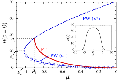
Figure 1: The maximum density $n_{\max}\equiv n(z=0)$ in the FT (flat-top) state, as per Eq. (14), and the PW (plane-wave) density are displayed as functions of $\mu$ by the red solid and blue dashed curves, respectively, for $\delta g/g=0.05$. In this case, Eq. (11) yields $n_{0}=36.025$ and $\mu_{0}=-0.900633$. The PW solution includes upper and lower branches corresponding to $n^{\pm}$, as given by Eq. (20), the lower one (marked by circles) being subject to the MI (modulational instability). The spinodal point is one with coordinates $\left(\mu_{c},n_{c}\right)$. For other values of $\delta g/g$, the plot can be generated from the present one by rescaling. The inset shows the density profile of the FT solution for $\delta g/g=0.05$ and $\mu=\mu_{0}+0.00001$, very close to the delocalization limit (the tranistion to PW).

The norm of the exact QD solutions given by Eqs. (13) is

$$N(\mu)=n_{0}\sqrt{-\frac{2}{\mu_{0}}}\left[\ln\left(\frac{1+\sqrt{\mu/\mu_{0}}}{\sqrt{1-\mu/\mu_{0}}}\right)-\sqrt{\frac{\mu}{\mu_{0}}}\right].$$ (15)

It satisfies the well-known Vakhitov-Kolokolov (VK) necessary stability criterion Vakhitov1973stationary ,

$$\frac{dN(\mu)}{d\mu}=-\frac{n_{0}}{\mu_{0}^{2}}\sqrt{-\frac{\mu}{2}}\frac{1}{1-\mu/\mu_{0}}<0,$$ (16)

due to $\mu_{0}<0$ and

$$0<\mu/\mu_{0}<1.$$ (17)

Full stability of the QD family has been verified by direct simulations of the evolution of perturbed QDs in the framework of Eq. (12).

It is relevant to mention that exact solution (13) is valid too at $\delta g/g<0$, when the cubic term in Eq. (12) is self-attractive, like the quadratic one. In that case, $\mu_{0}$ is positive, as per Eq. (11), while the chemical potential of the self-trapped state remains negative, as solution (13) may exist only at $\mu<0$. Then, it follows from Eq. (13) that the soliton-like mode exists for all values of $\mu<0$ (unlike the finite interval (17), in which the solution exists for $\delta g/g>0$), and it does not feature the FT shape. Rather, with the increase of $-\mu$, it demonstrates a crossover between the KdV-soliton shape $\sim\mathrm{sech}^{2}\left(\sqrt{-\mu/2}z\right)$ and the nonlinear-Schrödinger one, $\sim\mathrm{sech}\left(\sqrt{-2\mu}z\right)$. For $\delta g/g<0$, the $N(\mu)$ dependence for the soliton family carries over into the following form,

$$N(\mu)\biggl{|}_{\delta g<0}=n_{0}\sqrt{\frac{2}{\mu_{0}}}\left[\sqrt{-\frac{\mu}{\mu_{0}}}-\arctan\left(\sqrt{-\frac{\mu}{\mu_{0}}}\right)\right],$$ (18)

which is an analytical continuation of expression (15). This dependence also satisfies the VK criterion.

III.1.2 The plane-wave solution

The PW solution of Eq. (12 )can be presented in a form $\psi(z,t)=\sqrt{n}\exp\left(iK_{\text{PW}}z-i\mu t\right)$ with wavenumber $K_{\text{PW}}$ and constant density $n$, which determine the corresponding chemical potential:

$$\mu_{\text{PW}}=\frac{\delta g}{g}n-\frac{\sqrt{2}}{\pi}\sqrt{n}+\frac{1}{2}K_{\text{PW}}^{2}.$$ (19)

The Galilean invariance of Eq. (12) implies that any quiescent solution $\psi_{0}\left(z,t\right)$ generates a family of moving ones, with arbitrary velocity $c$. Therefore, $K_{\text{PW}}$ may be canceled by means of transformation $\psi_{c}\left(z,t\right)=\exp\left(icz-ic^{2}t/2\right)\psi_{0}\left(z-ct,t\right)$ with $c=-K_{\text{PW}}$.

For given $\mu$, Eq. (19) produces two different branches of the density as a function of $\mu$ (here, $K_{\text{PW}}=0$ is set):

$$\sqrt{n^{\pm}(\mu)}=\frac{1}{\sqrt{2}\pi}\frac{g}{\delta g}\pm\sqrt{\frac{1}{2\pi^{2}}\left(\frac{g}{\delta g}\right)^{2}+\frac{g}{\delta g}\mu}.$$ (20)

For $\delta g/g=0.05$, these branches are shown in Fig. 1. As follows from Eq. (20), they exist (for $\delta g/g>0$) above a minimum value of $\mu$: $\mu_{c}=-(2\pi^{2}\delta g/g)^{-1}=(9/8)\mu_{0}$, the respective density being

$$n_{c}=n^{\pm}(\mu_{c})=\frac{1}{2\pi^{2}}\left(\frac{g}{\delta g}\right)^{2}=\frac{9}{16}n_{0}.$$ (21)

Values $\mu=\mu_{c}$ and $n=n_{c}$ correspond to the spinodal point Petrov:2016 , and $n^{+}(\mu_{0})=n_{0}$ (see Eq. (13)). Note that the above-mentioned existence region of the soliton solution in terms of the chemical potential, $\mu_{0}<\mu<0$, lies completely inside that of the PW state, which is $\mu_{c}\leq\mu$. Thus, the soliton always coexists with the PW (this fact is also obvious in Fig. 1).

III.1.3 Modulational instability of the plane waves

Here, we aim to analyze the MI of PW solutions in the framework of the single-component GP equation (12) and demonstrate how the development of the MI can help to generate QDs. We perform the analysis for the PWs with zero wavenumber $K_{\text{PW}}=0$, which is sufficient due to the aforementioned Galilean invariance of the underlying equation.

A small perturbation is added to the stationary PW state as

$$\psi(z,t)=\left[\sqrt{n}+\delta\psi(z,t)\right]\exp\left(-i\mu t\right).$$ (22)

The substitution of this expression in Eq. (12) and linearization with respect to perturbation $\delta\psi$ leads to the corresponding Bogoliubov-de Gennes equation,

$$i\frac{\partial}{\partial t}\delta\psi=-\frac{1}{2}\frac{\partial^{2}}{\partial z^{2}}\delta\psi+\frac{\delta g}{g}n(\delta\psi+\delta\psi^{\ast})-\frac{\sqrt{n}}{\sqrt{2}\pi}(\delta\psi+\delta\psi^{\ast}).$$ (23)

By looking for perturbation eigenmodes with wavenumber $k$ and frequency $\Omega$,

$$\delta\psi=\zeta\cos(kz-\Omega t)+i\eta\sin(kz-\Omega t),$$ (24)

and real infinitesimal amplitudes $\zeta$ and $\eta$, Eq. (23) yields a dispersion relation for the eigenfrequencies:

$$\Omega^{2}=\frac{k^{4}}{4}+\left(\frac{\delta g}{g}n-\frac{\sqrt{n}}{\sqrt{2}\pi}\right)k^{2}.$$ (25)

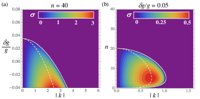
Figure 2: Color-coded values of the MI gain, $\sigma=\mathrm{Im}(\Omega)$, are displayed for fixed $n=40$ in (a), and for fixed $\delta g/g=0.05$ in (b). Note that panel (a) covers both signs of the cubic nonlinearity, $\delta g>0$ and $\delta g<0$. Solid and dashed white curves represent the MI boundary [Eq. (26)] and the peak value of the MI gain [Eq. (27)], respectively.

The MI takes place when $\Omega$ acquires an imaginary part. As follows from Eq. (25), this occurs when the density satisfies condition $n<[2\pi^{2}(\delta g/g)^{2}]^{-1}=n_{c}$ [see Eq. (21)], which corresponds to branch $n^{-}$ of the PW state. The instability region in terms of $k$ is given by

$$k^{2}<4\left(\frac{\sqrt{n}}{\sqrt{2}\pi}-\frac{\delta g}{g}n\right)\equiv k_{0}^{2}.$$ (26)

The MI gain $\sigma\equiv\left|\mathrm{Im}\Omega\right|$ is plotted in Fig. 2 versus $|k|$ and $\delta g/g$, for given density $n=40$ in panel (a), and versus $|k|$ and $n$, for given $\delta g/g=0.05$ in (b). It is easy to find from Eq. (25) that the largest gain is attained at wavenumber

$$k_{\max}=\frac{k_{0}}{\sqrt{2}},$$ (27)

with $k_{0}$ defined as per Eq. (26). Note that Fig. 2(a) includes the case of the self-attractive cubic nonlinearity, with $\delta g/g<0$, which naturally displays much stronger MI, as in this case it is driven by both the quadratic and cubic nonlinear terms. In fact, the extension of the MI chart to $\delta g/g<0$ makes it possible to complare the MI in the present system and its well-known counterpart in the setting with the fully attractive nonlinearity.

Comparing parameter values at which the QD solutions are predicted to appear, and the MI condition for the PW with the corresponding density, the MI is expected to provide a mechanism for the creation of the QDs. This is confirmed by direct simulations of the GP equation (12), as shown in Fig. 3. The PW with $n=10$ is taken as the input, so that it is subject to the MI for $\delta g/g=0.05$, as seen in Fig. 2(b). As shown in Fig. 3, small initial perturbations trigger the emergence of multiple-QD patterns (chains) at $t\geq 100$. For these parameters, we get $k_{\text{max}}\ =0.6508$ and $\sigma\left(k_{\text{max}}\right)=0.2118$, which determines the wavelength of the fastest growing modulation, $\lambda=2\pi/k_{\text{max}}\ \approx 9.66$, and the growth-time scale, $\tau=2\pi/\sigma\left(k_{\text{max}}\right)\approx 30$. The number of the generated droplets in Fig. 3 is consistent with estimate $L/\lambda\simeq 10$, where $L=100$ is the size of the simulation domain. We have checked that the number of generated droplets is approximately given by $L/\lambda$ for other values of parameters as well. This dynamical scenario is similar to those observed in other models in the course of the formation of soliton chains by MI of PWs Nguyen:2017Formation ; Everitt:2017Observation . The long-time evolution in Fig. 3(a) shows that the number of the droplets becomes smaller due to merger of colliding droplets into a single one, which agrees with dynamical properties of 1D QDs reported in Ref. Astrakharchik:2018Dynamics .

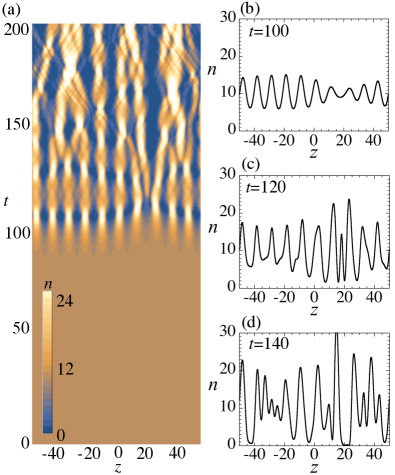
Figure 3: A typical example of the MI development, starting from an unstable PW state, with density $n=10$ and $\delta g/g=0.05$, which is subject to the MI, pursuant to Fig. 2. In (a), the spatiotemporal pattern of the evolution of the condensate density is shown. In the right-hand panels, cross sections of the density profiles are displayed at $t=100$ (b), $t=120$ (c), and $t=140$ (c). The simulations were performed in domain $-50<z<+50$ with $2500$ grid points and periodic boundary conditions.

To implement this mechanism of the generation of a chain of solitons in the experiment, i.e., make the density smaller than the critical value $n_{c}$, one may either apply interaction quench (by means of the Feshbach resonance), suddenly decreasing $\delta g/g$, as was done in recent experimental works for different purposes cabrera2018quantum ; Cheiney:2018Bright ; Semeghini:2018Self ; Strathclyde . Another option, which is specific to the 1D setting, is sudden decrease of density $n$ by relaxing the transverse trapping.

III.2 The two-component Gross-Pitaevskii model

In this section, we revert to the full two-component GP system (7), aiming to explore the formation of QD states in it. The two-component setting may include parameter imbalance between the two components, as indicated theoretically Petrov:2015 and observed experimentally cabrera2018quantum ; Cheiney:2018Bright ; Semeghini:2018Self ; long-lived . Here, we present the analysis of asymmetric QDs in two cases: (i) the two-component GP system with different populations, $N_{1}/N_{2}\neq 1$, and equal intra-component coupling strength, $g_{1}=g_{2}$ (i.e., $P=1$, see Eq. (8)), and (ii) the system with different intra-component coupling strengths, $g_{1}\neq g_{2}$ (i.e., $P\neq 1$). These options suggest a possibility to check the stability of the solutions of the symmetric system, reduced to the single-component form, against symmetry-breaking perturbations. That objective is relevant because, in the real experiment, scattering lengths of the self-interaction in the two components are never exactly equal cabrera2018quantum -2018arXiv181209151F . We address, first, an asymmetric single-droplet solution, and, subsequently, MI of the PW states in the two-component system.

Because, as said above, solutions with mutually proportional components (written as $\phi_{1}=K\phi_{2}$) are possible solely in the strictly symmetric setting, asymmetric QDs cannot be found in an exact analytical form. As shown in Appendix B [see Eqs. (48)-(54)], asymptotic analytical solutions can be obtained for strongly asymmetric states, with one equation replaced by its linearized version. In this section, we chiefly rely on numerical solution of Eq. (7).

III.2.1 Asymmetric QDs with unequal populations ($N_{1}\neq N_{2}$) for $g_{1}=g_{2}$ ($P=1$)

In the system with $P=1$ [see Eq. (8)], we calculated the droplet states as stationary solutions of Eq. (7) by means of the imaginary-time-evolution method with the Neumann’s boundary conditions, under the constraint that the norm is fixed in the first component, $\int_{-\infty}^{+\infty}dz|\psi_{1}(z)|^{2}=N_{1}$, while chemical potential $\mu_{2}$ is fixed in the other one, allowing its norm $N_{2}$ to vary.

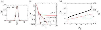
Figure 4: (a) Stationary weakly asymmetric (with respect to the two components) solutions of Eq. (7), obtained for $\mu_{2}=-0.4$ with fixed $N_{1}=100$. Dashed and solid curves display density profiles of the first ($n_{1}$) and second ($n_{2}$) components, respectively. (b) The semi-log plot of the density profiles of $n_{2}$ for $\mu_{2}=-0.4$, $-0.04$, and $0$ at $z>0$. (c) Dependences of $N_{2}$ (black dots: the left vertical axis) and asymmetry parameter $\delta_{21}$, defined as per Eq. (28) (the red dashed line pertaining to the right vertical axis), on $\mu_{2}$ for fixed $N_{1}=100$. The parameters are $P=1$ $(g_{1}=g_{2})$ and $\delta g/g=0.05$. The symmetric point with $N_{1}=N_{2}=100$ and $\delta_{21}=0$ corresponds to $\mu_{1}=\mu_{2}=-0.88878$.

Figure 4 displays essential features of weakly asymmetric droplets for $\delta g/g=0.05$ and fixed $N_{1}=100$. The symmetric (completely overlapping) solution with $N_{1}=N_{2}$ is found at $\mu_{1}=\mu_{2}=-0.88878$. When $\mu_{2}$ deviates from this value, profiles of the two components become slightly different, as shown in Fig. 4(a). The profiles of the droplet solution hardly change for different values of $\mu_{2}$, but panel 4(b) demonstrates that, at $\mu_{2}\to-0$, $\psi_{2}$ develops small-amplitude extended tails, which are absent in $\psi_{1}$. Due to the contribution of the tails, the approach of $\mu_{2}<0$ towards zero leads to the increase of norm $N_{2}$, as seen in Fig. 4(c). Note that the growth of $N_{2}(\mu_{2})$ at $\mu_{2}\rightarrow-0$ is opposite to the decay of the QD’s norm in the single-component model at $\mu\rightarrow-0$, cf. Eq. (15). At $\mu_{2}\geq 0$, the $\psi_{2}$ component undergoes delocalization, with its tails developing a nonzero background at $|z|\rightarrow\infty$, as seen in the density profile displayed in Fig. 4(b) for $\mu_{2}=0$, and norm $N_{2}(\mu_{2})$ diverging at $\mu_{2}\rightarrow-0$ in Fig. 4(c).

In Fig. 4(c), we also plot the parameter of the asymmetry between the two components, defined as

$$\delta_{21}=\frac{n_{2}(z=0)-n_{1}(z=0)}{n_{2}(z=0)+n_{1}(z=0)}.$$ (28)

It increases almost linearly with $\mu_{2}$, although its absolute value does not exceed $0.02$. Thus, the droplet tends to keep a nearly symmetric profile, with respect to the two components, in the symmetric system, even if the population imbalance is admitted. In fact, this circumstance makes the analysis self-consistent, as the use of the GP system with the LHY correction implies that the MF intra- and inter-component interactions nearly cancel each other, which is possible only if shapes of the two components are nearly identical.

III.2.2 Asymmetric QDs in the system with $P\neq 1$ ($g_{1}\neq g_{2}$)

Next, we consider the QDs for $P\neq 1$, setting $P>1$ without loss of generality. Then, the MF energy is minimized for $n_{2}>n_{1}$; the situation with $n_{1}>n_{2}$ can be considered too, replacing $P$ by $P^{-1}$.

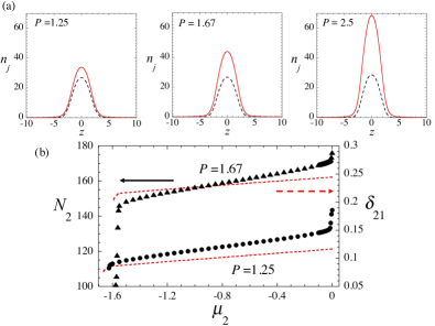
Figure 5: (a) Stationary solutions of Eq. (7), obtained for $\delta g/g=0.05$ and $N_{1}=100$. From the left panel to the right one, the parameter (8) is $P=1.25$, $1.67$, and $2.5$, and the chemical potential for the second component is $\mu_{2}=-0.018$, $-0.011$, and $-0.006$, respectively, just below the threshold above which the tails of $\psi_{2}$ extend to infinity. Dashed and solid curves represent the density of the first ($n_{1}$) and second ($n_{2}$) components. (b) Dependences of $N_{2}$ (black dots: the left vertical axis) and asymmetry parameter $\delta_{21}$, defined as per Eq. (28) (the red dashed line pertaining to the right vertical axis), on $\mu_{2}$ for fixed $N_{1}=100$ and $P=1.25$ or $P=1.67$.

Following the procedure similar to that employed in Sec. III.2.1, we produce QD solutions for $\delta g/g=0.05$, $N_{1}=100$, and several different values of $P$, varying $\mu_{2}$. In Fig. 5 (a), we plot density profiles for three different values of $P$. Naturally, the difference of the two components increases with the increase of $P$. In Fig. 5(b) we display $N_{2}$ and parameter $\delta_{21}$ [see Eq. (28)] of the asymmetric QDs for $P=1.25$ and $1.67$. All these states have been checked to be stable in time-dependent simulations.

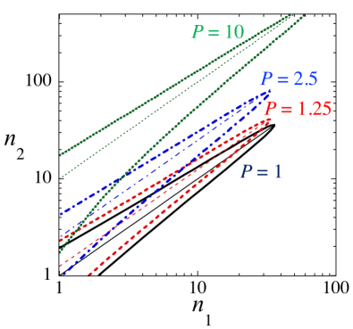
Figure 6: The negative-pressure region in the $\left(n_{1},n_{2}\right)$ plane for $\delta g/g=0.05$ and values of asymmetry parameter ( 8) $P=1$ (the solid curve), $1.25$ (dashed), $2.5$ (dashed-dotted), and $10$ (dotted). Boundaries are determined by the zero-pressure condition, as given by Eq. (31). The negative pressure, at which localized states may exist, occurs inside the boundaries. Thin lines represent relation $n_{2}=Pn_{1}$.

The density difference at the center of the droplet can be determined by the condition of the existence of the liquid phase in the free space. This condition is obtained by minimizing the grand-potential density $\mathcal{E}_{\text{1D}}\ -\mu_{1}\rho_{1}-\mu_{2}\rho_{2}$ Petrov:2016 ; Ancilotto2018 , which leads to the zero-pressure condition,

$$p(\rho_{1},\rho_{2}) =-\mathcal{E}_{\mathrm{1D}}+\sum_{j=1,2}\left(\frac{\partial\mathcal{E}_{\mathrm{1D}}}{\partial\rho_{j}}\right)\rho_{j}$$

$$\equiv-\mathcal{E}_{\text{{1D}}}\ +\mu_{1}\rho_{1}+\mu_{2}\rho_{2}=0.$$ (29)

From this, we obtain relation

$$\frac{(\sqrt{g_{1}}\rho_{1}-\sqrt{g_{2}}\rho_{2})^{2}}{2}+\frac{g\delta g(\sqrt{g_{2}}\rho_{1}+\sqrt{g_{1}}\rho_{2})^{2}}{(g_{1}+g_{2})^{2}}-\frac{\sqrt{m}}{3\pi\hbar}(g_{1}\rho_{1}+g_{2}\rho_{2})^{3/2}=0,$$ (30)

which can be rewritten in the scaled form as

$$\frac{P+GP^{-1}}{2}n_{1}^{2}+\frac{P^{-1}+GP}{2}n_{2}^{2}+(G-1)n_{1}n_{2}=\frac{1}{3\pi}\left(Pn_{1}+\frac{n_{2}}{P}\right)^{3/2}.$$ (31)

For given $n_{1}$, we solved Eq. (31) to find the respective value of $n_{2}$, which is shown in Fig. 6 for $\delta g/g=0.05$ and several values of $P$. There are two branches of the solutions, that enclose the negative-pressure region, in which QDs may exist. The maximum value of $n_{j}$ at the tip of the negative-pressure region corresponds to the density in the droplet’s FT segment. The ascending negative-pressure region for each $P$ nearly follows relation $n_{2}=Pn_{1}$, which is derived by the minimization condition for the dominant first term in Eq. (30) It is seen that a larger difference in the profiles of the two components occurs for larger $P$, as expected. Also, for given $n_{1}$, the negative-pressure region becomes wider with respect to $n_{2}$ for larger $P$ (note that the figure displays a log-log plot).

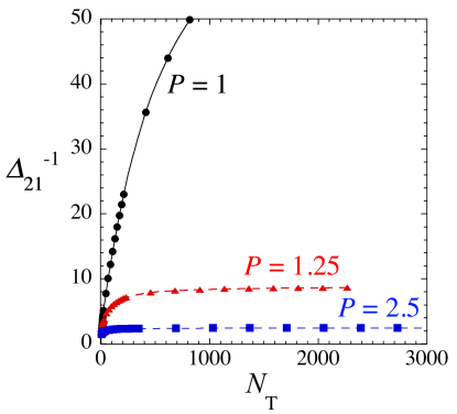
Figure 7: The inverse of the largest relative norm difference $\Delta_{21}$, up to which the asymmetric droplets exist [see Eq. (32)], shown as a function of the total number, $N_{\mathrm{T}}$, at different values of asymmetry parameter (8). Here we set $\delta g/g=0.05$.

As the QDs have a finite norm, it is relevant to characterize the asymmetry in terms of the norm, rather than density. Here, we aim to find a largest value of the norm difference,

$$\Delta_{21}=(N_{2}-N_{1})/N_{\mathrm{T}},$$ (32)

where $N_{\mathrm{T}}=N_{1}+N_{2}$ is the total norm, which admits the existence of the QDs. For given $N_{1}$, we obtain the upper bound for $N_{2}$ above which the solution becomes delocalized, and calculate the corresponding critical value of $\Delta_{21}$. The results are shown in Fig. 7. For the system with $P=1$ , the curve demonstrates an empirical dependence $\Delta_{21}\propto N_{\mathrm{T}}^{-\alpha}$ with exponent $\alpha\approx 0.58$. Accordingly, the asymmetry tends to vanish asymptotically for very “heavy” droplets, at $N_{\mathrm{T}}\leavevmode\nobreak\ \rightarrow\infty$. As the system becomes slightly asymmetric, with $P=1.25$, exponent $\alpha$ is significantly reduced for small $N_{\text{{T}}}$, and converges to a certain finite value at $N_{\text{{T}}}\ \rightarrow\infty$. Thus, it is again confirmed that values $P>1$ maintain conspicuous asymmetry between the QD’s components. Finally, strongly asymmetric non-FT (Gaussian-shaped Astrakharchik:2018Dynamics ) solutions can be obtained in an approximate analytical form for any value of $P$, as shown in Appendix B.

III.2.3 The MI of the asymmetric PW states

The MI of two-component asymmetric PWs is a relevant subject too. Such solutions are written as $\psi_{j}(z,t)=\sqrt{n_{j}}e^{-i\mu_{j}t},\,(j=1,2)$. The substitution of this in Eq. (7) yields

$$\mu_{1} = (P+GP^{-1})n_{1}+(-1+G)n_{2}-\frac{P}{\pi}\sqrt{Pn_{1}+\frac{n_{2}}{P}},\leavevmode\nobreak\ \leavevmode\nobreak\ \leavevmode\nobreak\$$

$$\mu_{2} = (P^{-1}+GP)n_{2}+(-1+G)n_{1}-\frac{1}{\pi P}\sqrt{Pn_{1}+\frac{n_{2}}{P}}.$$ (33)

Accordingly, in the symmetric system with $P=1$, densities of the asymmetric PW state are expressed in terms of the chemical potentials as

$$\begin{split}n_{j}&=\frac{1}{4}\left[\frac{1}{\pi^{2}G^{2}}+\frac{\mu_{1}+\mu_{2}}{G}+(-1)^{j+1}(\mu_{1}-\mu_{2})\right]\\ &\pm\frac{\sqrt{1+2\pi^{2}G(\mu_{1}+\mu_{2})}}{4\pi^{2}G^{2}}.\end{split}$$ (34)

We introduce the perturbation around the PW states as

$$\psi_{j}(z,t)=\left[\sqrt{n_{j}}+\delta\psi_{j}(z,t)\right]e^{-i\mu_{j}t},$$ (35)

$$\delta\psi_{j}=\zeta_{j}\cos(kz-\Omega t)+i\eta_{j}\sin(kz-\Omega t),$$ (36)

with infinitesimal amplitudes $\zeta_{j}$ and $\eta_{j}$, cf. Eq. (24). The substitution of this in Eqs. (7) and the linearization with respect to $\zeta_{j}$ and $\eta_{j}$ yields the dispersion equation for the perturbation:

$$\begin{split}\Omega_{\pm}^{2}=\frac{k^{2}}{4}\left[k^{2}+2(P_{1}+P_{2}-Q_{1}-Q_{2})\right]\\ \pm\frac{k^{2}}{2}\sqrt{(P_{1}-P_{2}-Q_{1}+Q_{2})^{2}+4(R-S)^{2}},\end{split}$$ (37)

where

$$P_{1}=(P+GP^{-1})n_{1},\quad P_{2}=(P^{-1}+GP)n_{2},$$

$$Q_{1}=\frac{P^{2}n_{1}}{2\pi\sqrt{Pn_{1}+P^{-1}n_{2}}},\quad Q_{2}=\frac{P^{-2}n_{2}}{2\pi\sqrt{Pn_{1}+P^{-1}n_{2}}}.$$ (38)

$$R=(-1+G)\sqrt{n_{1}n_{2}},\quad S=\frac{\sqrt{n_{1}n_{2}}}{2\pi\sqrt{Pn_{1}+P^{-1}n_{2}}},$$

For $P=1$ and $n_{1}=n_{2}$, these results reproduce Eq. (25) for the $\Omega_{-}$ branch. A parameter region in which at least one squared eigenfrequency $\Omega_{\pm}^{2}$ is negative gives rise to the MI of the two-component state.

III.2.4 The MI for $P=1$

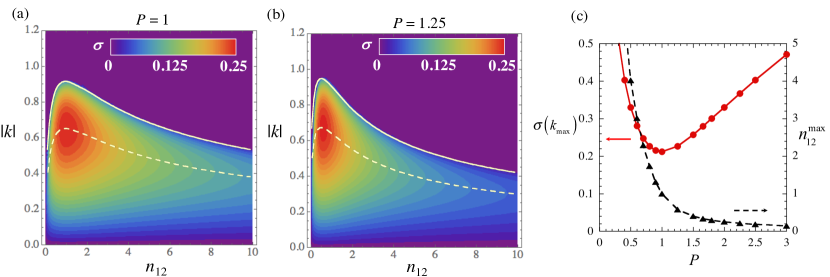
Figure 8: Color-coded values of the MI gain, $\sigma=\mathrm{Im}(\Omega)$, for asymmetric PWs, as calculated from Eq. (37) in the plane of wave number $|k|$ and density ratio $n_{12}=n_{1}/n_{2}$, are displayed for (a) $P=1$ and (b) $P=1.25$ with fixed $\delta g/g=0.05$ and $(n_{1}+n_{2})/2=10$. The solid and dashed white curves represent the MI boundary $k=k_{0}$ and the peak value of the MI gain at $k=k_{\text{max}}\ =k_{0}/\sqrt{2}$, respectively. In (c), we plot $\sigma(k_{\text{max}})$ (circles) and $n_{12}^{\text{max}}$ (triangles) versus $P$.

In Fig. 8, we plot the gain spectrum $\sigma=\mathrm{Im}(\Omega)$ for the asymmetric PWs in the symmetric system with $P=1$ and $\delta g/g=0.05$, in the plane of wavenumber $k$ and density ratio $n_{12}=n_{2}/n_{2}$. For the consistency with the single-component situation displayed in Fig. 3, we here fix the total density as $(n_{1}+n_{2})/2=10$. For given $n_{12}$, the MI occurs at $|k|<k_{0}$, and the gain attains its maximum at $k=k_{\text{max}}=k_{0}/\sqrt{2}$. The largest gain is obtained at equal densities, $n_{12}=1$. Both the $k$-band of the instability and magnitude of the gain slowly decrease as the deviation of $n_{12}$ from unity increases. This means that the MI occurs in the PW states with a large density difference, thus giving rise to the formation of solitons with large asymmetry even for equal intra-component MF interaction strengths, $P=1$ [see Eq. (8)] .

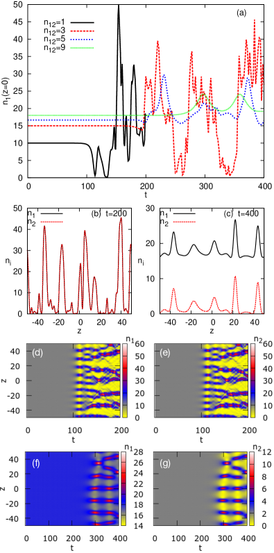
Figure 9: Numerically simulated development of the MI of asymmetric PW states in the two-component system, with $P=1$ and $\delta g/g=0.05$ . The initial PW states are taken with fixed total density, $(n_{1}+n_{2})/2=10$. (a) The evolution of the central density of the first component, $n_{1}(z=0)$, for different density ratios in the two components, $n_{12}=n_{1}/n_{2}$. (b,c) Snapshots of density profiles for the cases of (b) $n_{12}\equiv n_{1}/n_{2}=1$ at $t=200$ and (c) $n_{12}=9$ at $t=400$. Panels (d,e) and (f,g) are top views of the spatiotemporal evolution of the densities, $n_{1}\left(z,t\right)$ and $n_{2}(z,t)$, for $n_{12}=1$ and $n_{12}=9$, respectively. Simulations were performed in the domain $-50\leq z\leq+50$ with $2048$ grid points, subject to periodic boundary conditions. In this figure and in Fig. 10, the scaled time unit corresponds to $\sim 1$ $\mu$s in physical units.

In Fig. 9 we display typical examples of the numerically simulated development of the MI in the symmetric two-component system with $P=1$ and population imbalance. Figure 9(a) shows the evolution of central-point values of the density of the first component, $n_{1}(z=0)$, for different values of the density ratio, $n_{12}=n_{1}/n_{2}$. Time required for the actual onset of the instability increases with the increase in $n_{12}$, as is clearly shown by the density-plot evolution in Figs. 9(d,e) for $n_{12}=1$ and (f,g) for $n_{12}=9$. This observation can be understood in terms of the MI gain $\sigma$, as shown in Fig. 8(c), where $\sigma$ at $k=k_{\text{max}}$ becomes smaller with increasing $n_{12}$.

Spatial profiles at fixed time, which are plotted in Fig. 9(b,c) for these two cases, show fragmentation of the profiles into sets of localized structures. The decrease in the number of fragments with the increase of $n_{12}$ is explained by the decrease of $k_{\max}$, see Fig. 8(a). For $n_{12}=1$, the results are the same as in the single-component case, as coinciding profiles in the two components of the symmetric system are stable against spontaneous symmetry breaking. On the other hand, when $n_{12}\neq 1$ an in-phase two-component localized structure appears, keeping the initial density imbalance. Since one can select an arbitrary ratio of densities of the two components for the initial PW state, a highly asymmetric structure, like the one displayed in Fig. 9(c), may emerge even for $P=1$, as a result of the MI-induced nonlinear evolution.

III.2.5 The MI for $P\neq 1$

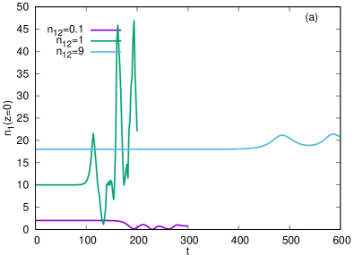
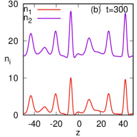
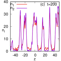
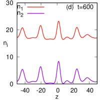
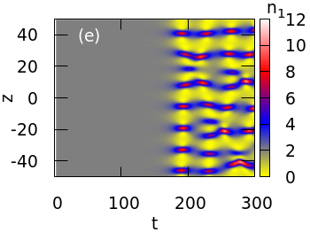
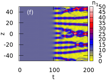
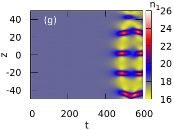
Figure 10: Numerically simulated development of the modulational instability in the two-component system with $\delta g/g=0.05$ and $P=1.25$. The initial PW states are taken with a fixed total density, $(n_{1}+n_{2})/2=10$. (a) The evolution of the central density of the first component, $n_{1}(z=0)$, for different density ratios in the two components, $n_{12}=n_{1}/n_{2}$. (b-d) Snapshots of density profiles for the cases of (b) $n_{12}\equiv n_{1}/n_{2}\sim 0.1$ at $t=300$, (c) $n_{12}=1$ at $t=200$ and (d) $n_{12}=9$ at $t=600$. Panels (e-g) represent the top view of the spatiotemporal evolution of the densities, $n_{1}\left(z,t\right)$, corresponding to (b-d), respectively (the evolution of $n_{2}\left(z,t\right)$ shows similar patterns). Simulations were performed in the domain $-50\leq z\leq+50$ with $2048$ grid points, subject to periodic boundary conditions.

Figure 8(b) represents the MI gain for $P=1.25$ and a fixed total density, $(n_{1}+n_{2})/2=10$, in the case of slightly different strengths of the intra-component repulsion. The peak value of the MI gain is attained at $n_{12}=n_{12}^{\text{max}}=0.577$, below the equal-densities point $n_{12}=1$. This is consistent with the fact that, at $P>1$, unequal values $n_{1}<n_{2}$ are suitable to the formation of an asymmetric soliton structure, as seen in Fig. 5(a). In Fig. 8(c), we plot the peak MI gain, $\sigma(k_{\text{max}})$, along with the respective value of the density ratio, $n_{12}^{\text{max}}$, as a function of $P$. Value $n_{12}^{\text{max}}$ monotonously decreases as a function of $P$, while the peak gain attains a minimum at $P=1$.

In Fig. 10, we present the development of the MI in the two-component system for $P=1.25$ and a fixed total density, $(n_{1}+n_{2})/2=10$. Figure 10(a) displays the evolution of the central-point density of the first component, $n_{1}(z=0)$, for different values of the density ratio, $n_{12}=n_{1}/n_{2}$. It shows that time required for the development of the MI increases with the increase in the asymmetry of the density. This is also made evident by the density plots of the temporal evolution of the first component, shown in Figs. 10(e-g). This result is consistent with Eq. (37), which shows a decrease of the MI gain with the increase of the asymmetry even for $P\neq 1$. Spatial profiles at fixed time, displayed in Fig. 10(b-d), show fragmentation of the profiles. Figure 10(c) clearly indicates that, even for $n_{12}=1$, the MI generates asymmetric droplet-like structures similar to Fig. 5(a), where the complete overlapping of the two densities does not occur.

IV Conclusion

The main purpose of this work is to associate the MI (modulation instability) of plane waves (PWs) to the mechanism of the creation of QDs (quantum droplets) in the system described by the coupled GP (Gross-Pitaevskii) equations including the LHY (Lee-Huang-Yang) terms in the 1D setting. This system is the model of weakly interacting binary Bose gases with approximately balanced interactions between the intra-component self-repulsion and the inter-component attraction. We have investigated, analytically and numerically, the MI of the lower branch of PW states in both symmetric (effectively single-component) and asymmetric (two-component) GP systems, and ensuing formation of a chain of droplet-like states. In particular, numerical solution for QDs which are asymmetric with respect to the two components are obtained, both in the system with equal repulsion strengths but unequal populations in the two components, and in the one with different self-repulsion strengths. The results corroborate that the previously known symmetric states are robust against symmetry-breaking disturbances.

These predictions can be tested experimentally by preparing uniform binary Bose gases with equal or different densities of two components, and suddenly reducing the strength of the effective MF (mean-field) interaction by means of the Feshbach-resonance quench, in order to enhance the relative strength of the LHY terms. In particular, for typical values of physical parameters, an estimate of the characteristic time of the modulation instability growth for typical values of the physical parameters is $\sim 1$ $\mu$s. This time is much smaller than a typical lifetime of the droplet, which is $\gtrsim 100$ $\mu$s cabrera2018quantum -Semeghini:2018Self , long-lived , thus making the observation of the MI feasible. The present analysis being restricted to the 1D setting, effects of the tight transverse confinement and crossover to the 3D configuration crossover ; Ilg:2018 ; Edler:2018 deserves further consideration.

Appendix A Other exact solutions for the single-component GP equation

Here we briefly list other types of exact solutions of the single-component equation (12), in addition to the FT and PW solutions (13) and (22) which were considered in detail above (solutions to Eq. (12) in the form of dark and anti-dark solitons were reported in Ref. Milivoj ).The stability of a majority of these solutions is not addressed here, as it should be a subject for a separate work.

A.1 $\delta g/g>0$

In the case of comparable quadratic self-attraction and cubic repulsion in Eq. (12) with $\delta g>0$, exact spatially-periodic solutions with odd parity can be expressed in terms of the Jacobi’s elliptic sine, whose modulus $q$ is an intrinsic parameter of the family:

$$\psi(z,t)=\exp\left(-i\mu_{\text{sn}}t\right)[A\leavevmode\nobreak\ \text{sn}(\beta z,q)+B],$$ (39)

where

$$B =\frac{\sqrt{2}}{3\pi}\frac{g}{\delta g}>0,\quad A=\sqrt{\frac{2}{1+q^{2}}}B>0,$$ (40)

$$\quad\mu_{\text{sn}} =-2\frac{\delta g}{g}B^{2}\,<0,\quad\beta^{2}=\frac{2}{\left(1+q^{2}\right)}\frac{\delta g}{g}B^{2}.$$

In the limit of $q\rightarrow 1$, solution (39) goes over into the kink (the same as found in Ref. Milivoj ),

$$\psi(z,t)=\exp\left(-i\mu_{\mathrm{kink}}t\right)[A\tanh(\beta z)+B]\,,$$ (41)

with parameters

$$A=B=\frac{\sqrt{2}}{3\pi}\frac{g}{\delta g}>0,\quad\mu_{\mathrm{kink}}=-2\frac{\delta g}{g}B^{2},\quad\beta^{2}=\frac{\delta g}{g}B^{2}.$$

A.2 $\delta g/g<0$

In the case when the inter-species MF attraction is stronger than the intra-species repulsion, resulting in $\delta g<0$, spatially-periodic solutions are expressed in terms of even Jacobi’s elliptic functions, $\mathrm{dn}(x,q)$ and $\mathrm{cn}(x,q)$. First, it is

$$\psi(z,t)=\exp\left(-i\mu_{\text{dn}}t\right)[A{\ }\text{dn}(\beta z,q)+B],$$ (42)

with the elliptic modulus taking all values $0<q<1$, other parameters being

$$B =\frac{\sqrt{2}}{3\pi}\frac{g}{\delta g}<0,\quad A=-\sqrt{\frac{2}{2-q^{2}}}B>0,$$ (43)

$$\quad\mu_{\mathrm{dn}} =-2B^{2}\frac{\delta g}{g}>0,\quad\beta^{2}=-\frac{2}{\left(2-q^{2}\right)}\frac{\delta g}{g}B^{2}.$$

The second solution is expressed in terms of the elliptic cosine, with $q^{2}>1/2$:

$$\psi(z,t)=\exp\left(-i\mu_{\text{cn}}t\right)[A{\ }\text{cn}(\beta z,q)+B]\,,$$ (44)

$$B =\frac{\sqrt{2}}{3\pi}\frac{g}{\delta g}<0,\quad A=-\sqrt{\frac{2}{2q^{2}-1}}B>0,$$ (45)

$$\quad\mu_{cn} =-2\frac{\delta g}{g}B^{2}\,>0,\quad\beta^{2}=-\frac{2}{(2q^{2}-1)}\frac{\delta g}{g}B^{2}.$$

In the limit of $q\rightarrow 1$, both solutions (42) and (44) carry over into a state of the “bubble” type barashenkov1993stability , which changes the sign at two points (the same solution was reported as an “W-shaped soliton” in Ref. Milivoj ):

$$\psi(z,t)=\exp\left(-i\mu_{\mathrm{bubble}}t\right)[A\text{sech}(\beta z)+B],$$ (46)

with parameters

$$B=\frac{\sqrt{2}}{3\pi}\frac{g}{\delta g}<0,\quad A=-\sqrt{2}B\,>0,$$ (47)

$$\quad\mu_{\mathrm{\ bubble}}=\beta^{2}=-2\frac{\delta g}{g}B^{2}>0.$$

Appendix B Analytical solutions for strongly asymmetric fundamental and dipole states

Here we consider analytical solutions of Eqs. (7) with strong asymmetry, $N_{1}\ll N_{2},$ which can be found under small-amplitude conditions, $n_{1}(z=0)\ll n_{2}(z=0)\ll n_{0}$. Then, cubic terms may be neglected in Eqs. (7), and approximation $\sqrt{P|\psi_{1}|^{2}+P^{-1}|\psi_{2}|^{2}}\approx P^{-1/2}\left|\psi_{2}\right|$ is used to simplify Eq. (7) to the following equations for stationary states (9):

$$\mu_{1}\phi_{1} =-\frac{1}{2}\frac{d^{2}\phi_{1}}{dz^{2}}-\frac{\sqrt{P}}{\pi}\phi_{2}\phi_{1},$$ (48)

$$\mu_{2}\phi_{2} =-\frac{1}{2}\frac{d^{2}\phi_{2}}{dz^{2}}-\frac{1}{\pi P^{3/2}}\phi_{2}^{2}.$$ (49)

Although this case is somewhat formal, in terms of the underlying concept of the quantum droplets, which is essentially based on the competition of residual MF and LHY terms, it is interesting to consider it too.

The soliton solution of Eq. (49) is obvious,

$$\phi_{2}(z)=\frac{3\pi}{2}\left(-\mu_{2}\right)\frac{P^{3/2}}{\cosh^{2}\left(\sqrt{-\mu_{2}/2}z\right)}$$ (50)

[solution (13) takes essentially the same form in the limit of $|\mu|\ll\mu_{0}$]. Then, the substitution of Eq. (50) in Eq. (48) makes it tantamount to the linear Schrödinger equation with the Pöschl-Teller potential LL . The ground-state (GS) solution of Eq. (48) for $\phi_{1}$, with arbitrary amplitude $\phi_{1}^{(0)}$,

$$\left(\phi_{1}(z)\right)_{\mathrm{GS}}=\frac{\phi_{1}^{(0)}}{\left[\cosh\left(\sqrt{-\mu_{2}/2}z\right)\right]^{\gamma}},$$ (51)

exists with

$$\gamma=\frac{1}{2}\left(\sqrt{24P^{2}+1}-1\right),$$ (52)

and eigenvalue

$$\left(\mu_{1}\right)_{\mathrm{GS}}=\left(\sqrt{24P^{2}+1}-1\right)^{2}\ \frac{\mu_{2}}{16}.$$ (53)

In this case, the QD solutions are quasi-Gaussian objects Astrakharchik:2018Dynamics . Note that, in the symmetric system with $P=1$, Eqs. (52) and (53) yield $\gamma=2$ and $\left(\mu_{1}\right)_{\mathrm{GS}}=\mu_{2}$, i.e., the eigenmode and eigenvalue coincide with their counterparts in the soliton solution (50), while they are different in the asymmetric system, the GS level lying below or above the chemical potential of soliton (50) at $g_{1}>g_{2}$ and $g_{1}<g_{2}$, respectively.

In Fig. 11 we compare a typical asymptotic solution given by Eqs. (50) and (51) with a numerically obtained GS solution for the same values of the parameters. It is seen that the analytical and numerical results match well.

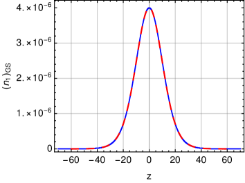
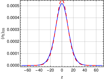
Figure 11: Comparison of the asymptotic analytical solutions, given by Eqs.  (50) and (51), with their numerically obtained counterparts. The density of the first ($n_{1}$) and second ($n_{2}$) components are displayed in top and bottom panels, respectively. Solid blue lines represent the numerical results, while dashed red lines represent the analytical solution. Here, parameters are $\delta g/g=0.05$, $N_{1}=0.0001067$, $N_{2}=0.0148044$ and $(\mu_{2})_{\mathrm{GS}}=\mu_{2}=-0.005$.

Further, it is also possible to produce the first excited state of Eq. (48) in the form of the dipole (antisymmetric) mode with an arbitrary amplitude:

$$\left(\phi_{1}(z)\right)_{\mathrm{dip}}=\frac{\phi_{1}^{(0)}\sinh\left(\sqrt{-\mu_{2}/2}z\right)}{\left[\cosh\left(\sqrt{-\mu_{2}/2}z\right)\right]^{\gamma}},$$ (54)

where $\gamma$ is the same as in Eq. (52), the respective eigenvalue being

$$\left(\mu_{1}\right)_{\mathrm{dip}}=\left(\sqrt{24P^{2}+1}-3\right)^{2}\frac{\mu_{2}}{16},$$ (55)

which is obviously higher than its GS counterpart (53) [at $P=1$, Eq. (55) yields $\left(\mu_{1}\right)_{\mathrm{dip}}=\mu_{2}/4$, and $\left(\mu_{1}\right)_{\mathrm{dip}}$ falls below $\mu_{2}$ for $P>\sqrt{2}$]. Unlike the GS, the dipole mode exists not at all values of $P$, but only for $P>\sqrt{1/3}$. Exactly at $P=\sqrt{1/3}$, one has $\left(\mu_{1}\right)_{\mathrm{dip}}=0$, and the dipole mode (54), with $\gamma=1$, is a delocalized one, $\sim\tanh\left(\sqrt{-\mu_{2}/2}z\right)$.

Linear Schrödinger equation (48) with the Pöschl-Teller potential may give rise to higher bound states of integer order $\nu$ as well, with eigenvalues

$$\left(\mu_{1}\right)_{\nu}=\left(\sqrt{24P^{2}+1}-\left(1+2\nu\right)\right)^{2}\frac{\mu_{2}}{16},$$ (56)

where $\nu=0$ and $1$ correspond to Eqs. (53) and (55), respectively, the $\nu$-th spate existing at $P^{2}>\nu\left(\nu+1\right)/6$. The number of such solutions is always finite.

Unlike solutions considered in Appendices A and C, the stability of solutions given by Eqs. (50)-(56) is obvious.

Appendix C Other exact solutions in the case of $N_{1}\ll N_{2}$

Here we provide periodic solutions to the semi-linear system of Eqs. (48) and (49) in terms of Jacobi elliptic functions. In the limit of $q\rightarrow 1$, they go over into solutions given in the main text, in the form of Eqs. (50), (51) and (54).

C.1 Solution of Eq. (49)

An exact periodic solution of Eq. (49) with the quadratic nonlinearity is

$$\phi_{2}=A[\text{dn}^{2}(\beta z,q)+p]\,,$$ (57)

with

$$\begin{split}\beta^{2}&=-\frac{\mu_{2}}{2\sqrt{1-q+q^{2}}},\quad A=-\frac{3\pi\mu_{2}P^{3/2}}{2\sqrt{1-q+q^{2}}},\\ \quad p&=\frac{-(2-q)+\sqrt{1-q+q^{2}}}{3}.\end{split}$$ (58)

In the limit of $q\rightarrow 1$, solution (57) goes over into solution (50). Note that $p$ is vanishing in this limit, according to Eq. (58).

C.2 Solutions of Eq. (48)

We now show that, with $\phi_{2}$ given by Eq. (57), linear equation (48) $\phi_{1}$ has several particular solutions depending on the value of $P$.

Solutions For $P^{2}=1/3$

C.2.1 Solution I

It is easy to check that

$$\phi_{1}=\phi_{1}^{(0)}\text{dn}(\beta z,q)$$ (59)

is an exact solution to Eq. (48), provided that

$$P^{2}=\frac{1}{3},\quad\mu_{1}=\left(\frac{\mu_{2}}{12}\right)\frac{2-q+2\sqrt{1-q+q^{2}}}{\sqrt{1-q+q^{2}}}\,.$$

C.2.2 Solution II

$$\phi_{1}=\phi_{1}^{(0)}\text{cn}(\beta z,q)$$ (60)

is an exact solution to Eq. (48), provided that

$$P^{2}=\frac{1}{3},\quad\mu_{1}=\left(\frac{\mu_{2}}{12}\right)\frac{2q-1+2\sqrt{1-q+q^{2}}}{\sqrt{1-q+q^{2}}}\,.$$

In the limit of $q\rightarrow 1$, solutions I and II go over into the solution Eq. (51) with $\gamma=1$ and $\mu_{1}=\mu_{2}/4$.

C.2.3 Solution III

$$\phi_{1}=\phi_{1}^{(0)}\text{sn}(\beta z,q)$$ (61)

is an exact solution to Eq. (48), provided that

$$P^{2}=\frac{1}{3}\,,\quad\mu_{1}=\left(\frac{\mu_{2}}{12}\right)\frac{2\sqrt{1-q+q^{2}}-(1+q)}{\sqrt{1-q+q^{2}}}\,.$$

In the limit of $q\rightarrow 1$, solution III goes over into the solution Eq. (54) with $\gamma=1$ and $\mu_{1}=0$.

Solutions For $P^{2}=1$

C.2.4 Solution IV

It is easy to check that

$$\phi_{1}=\phi_{1}^{(0)}[\text{dn}^{2}(\beta z,q)+p]\,$$ (62)

is an exact solution to Eq. (48), provided that

$$P^{2}=1,\quad\mu_{1}=\mu_{2}\,.$$

C.2.5 Solution V

$$\phi_{1}=\phi_{1}^{(0)}\text{cn}(\beta z,q)\text{dn}(\beta z,q)\,$$ (63)

is an exact solution to Eq. (48), provided that

$$P^{2}=1,\quad\mu_{1}=\left(\frac{\mu_{2}}{2}\right)\frac{q+\sqrt{1-q+q^{2}}}{\sqrt{1-q+q^{2}}}\,.$$

In the limit $q=1$, solutions IV and V go over into solution Eq. (51) with $\gamma=2$ and $\mu_{1}=\mu_{2}$.

C.2.6 Solution VI

$$\phi_{1}=\phi_{1}^{(0)}\text{sn}(\beta z,q)\text{dn}(\beta z,q)\,$$ (64)

is an exact solution to Eq. (48), provided that

$$P^{2}=1\,,\quad\mu_{1}=\left(\frac{\mu_{2}}{4}\right)\frac{3(1-q)+\sqrt{1-q+q^{2}}}{\sqrt{1-q+q^{2}}}\,.$$

C.2.7 Solution VII

$$\phi_{1}=\phi_{1}^{(0)}\text{sn}(\beta z,q)\text{cn}(\beta z,q)\,$$ (65)

is an exact solution to Eq. (48), provided that

$$P^{2}=1\,,\quad\mu_{1}=\left(\frac{\mu_{2}}{4}\right)\frac{2\sqrt{1-q+q^{2}}-(2-q)}{\sqrt{1-q+q^{2}}}\,.$$

In the limit of $q\rightarrow 1$, solutions VI and VII go over into (54), with $\gamma=2$ and $\mu_{1}=\mu_{2}/4$.

References

- (1) L. Pitaevskii and S. Stringari, Bose-Einstein condensation and superfluidity; Oxford University Press: Oxford, 2016.
- (2) C. Pethick and H. Smith, Bose-Einstein condensation in dilute gases; Cambridge University Press: Cambridge, 2002.
- (3) D. S. Petrov, Quantum Mechanical Stabilization of a Collapsing Bose-Bose Mixture, Phys. Rev. Lett. 2015, 115, 155302.
- (4) T. D. Lee, K. Huang, and C. N. Yang, Eigenvalues and Eigenfunctions of a Bose System of Hard Spheres and Its Low-Temperature Properties, Phys. Rev. 1957, 106, 1135-1145.
- (5) D. S. Petrov, and G. E. Astrakharchik, Ultradilute low-dimensional liquids, Phys. Rev. Lett. 2016, 117, 100401.
- (6) Y. Li, Z. Luo, Y. Lio, Z. Chen, C. Huang,S. Fu, H. Tan, and B. A. Malomed, Two-dimensional solitons and quantum droplets supported by competing self-and cross-interactions in spin-orbit-coupled condensates, New J. Phys. 2017, 19, 113043.
- (7) A. Cappellaro, T. Macrí, G. F. Bertacco and L. Salasnich, Equation of state and self-bound droplet in Rabi-coupled Bose mixtures, Sci. Rep. 2017, 7, 13358.
- (8) N. B. Jørgensen, G. M. Bruun, and J. J. Arlt, Dilute fluid governed by quantum fluctuations, Phys. Rev. Lett. 2018, 121, 17, 173403.
- (9) V. Cikojević, K. Dželalija, P. Stipanović, and L. Vranjes Markić, and J. Boronat, Ultradilute quantum liquid drops, Phys. Rev. B 2018, 97, 140502(R).
- (10) A. Cappellaro, T. Macrí, and L. Salasnich, Collective modes across the soliton-droplet crossover in binary Bose mixtures, Phys. Rev. A 2018, 97, 053623.
- (11) Y. V. Kartashov, B. A. Malomed, L. Tarruell, and L. Torner, Three-dimensional droplets of swirling superfluids, Phys. Rev. 2018, 98, 013612.
- (12) P. Zin, M. Pylak, T. Wasak, M. Gajda, and Z. Idziaszek, Quantum Bose-Bose droplets at a dimensional crossover, Phys. Rev. A 2018, 98, 051603(R).
- (13) Y. Li, Z. Chen, Z. Luo, C. Huang, H. Tan, W. Pang, and B. A. Malomed, Two-dimensional vortex quantum droplets, Phys. Rev. A 2018, 98, 063602.
- (14) F. Ancilotto, M. Barranco, M. Guilleumas, and M. Pi, Self-bound ultradilute Bose mixtures within local density approximation, Phys. Rev. A 2018, 98, 053623.
- (15) B. Liu, H.-F. Zhang, R.-X. Zhong, X.-L. Zhang, X.-Z. Qin, C. Huang, Y.-Y. Li, and B. A. Malomed, Symmetry breaking of quantum droplets in a dual-core trap, Phys. Rev. A 2019 99, 053602.
- (16) E. Chiquillo, Low-dimensional self-bound quantum Rabi-coupled bosonic droplets, Phys. Rev. A 2019, 99, 051601(R).
- (17) A. Tononi, Y. Wang, L. Salasnich, Quantum solitons in spin-orbit-coupled Bose-Bose mixtures, Phys. Rev. A 2019, 99, 063618.
- (18) Y. V. Kartashov, B. A. Malomed, and L. Torner, Metastability of Quantum Droplet Clusters, Phys. Rev. Lett. 2019, 122, 193902.
- (19) X. Zhang, X. Xu, Y. Zheng, Z. Chen, B. Liu, C. Huang, B. A. Malomed, and Y. Li, Semidiscrete quantum droplets and vortices, Phys. Rev. Lett. 2019, 123, 133901.
- (20) G. E. Astrakharchik, and B. A. Malomed, Dynamics of one-dimensional quantum droplets, Phys. Rev. A 2018, 98, 013631 (2018).
- (21) C. Cabrera, L. Tanzi, J. Sanz, B. Naylor, P. Thomas, P. Cheiney, and L. Tarruell, Quantum liquid droplets in a mixture of Bose-Einstein condensates, Science 2018, 359, 301-304.
- (22) P. Cheiney, C. R. Cabrera, J. Sanz, B. Naylor, L. Tanzi, and L. Tarruell, Bright Soliton to Quantum Droplet Transition in a Mixture of Bose-Einstein Condensates, Phys. Rev. Lett. 2018, 120 135301 .
- (23) G. Semeghini, G. Ferioli, L. Masi, C. Mazzinghi, L. Wolswijk, F. Minardi, M. Modugno, G. Modugno, M. Inguscio, and M. Fattori, Self-Bound Quantum Droplets of Atomic Mixtures in Free Space, Phys. Rev. Lett. 2018, 120, 235301.
- (24) G. Ferioli, G. Semeghini, L. Masi, G. Giusti, G. Modugno, M. Inguscio, A. Gallemi, A. Recati, and M. Fattori, Collisions of self-bound quantum droplets, Phys. Rev. Lett. 2019, 122, 090401.
- (25) Y. Kartashov, G. Astrakharchik, B. Malomed, and L. Torner, Frontiers in multidimensional self-trapping of nonlinear fields and matter, Nature Rev. Phys. 2019, 1, 185-197.
- (26) I. Ferrier-Barbut, Ultradilute Quantum Droplets, Physics Today 2019, 72, No. 4, 46-52.
- (27) C. D’Errico, A. Burchianti, M. Prevedelli, L. Salasnich, F. Ancilotto, M. Modugno, F. Minardi, and C. Fort, Observation of quantum droplets in a heteronuclear bosonic mixture, Phys. Rev. Research 2019, 1, 033155.
- (28) H. Kadau, M. Schmitt, M. Wentzel, C. Wink, T. Maier, I. Ferrier-Barbut, and T. Pfau, Observing the Rosenzweig instability of a quantum ferrofluid, Nature 2016, 530, 194-197.
- (29) M. Schmitt, M. Wenzel, F. Böttcher, I. Ferrier-Barbut and T. Pfau, Self-bound droplets of a dilute magnetic quantum liquid, Nature 2016, 539, 259-262.
- (30) F. Wächtler, and L. Santos, Quantum filaments in dipolar Bose-Einstein condensates, Phys. Rev. A 2016, 93 061603(R).
- (31) I. Ferrier-Barbut, H. Kadau, M. Schmitt, M. Wenzel, and T. Pfau, Observation of Quantum Droplets in a Strongly Dipolar Bose Gas, Phys. Rev. Lett. 2016, 116, 215301.
- (32) F. Wächtler, and L. Santos, Ground-state properties and elementary excitations of quantum droplets in dipolar Bose-Einstein condensates, Phys. Rev. A 2016, 94, 043618.
- (33) D. Baillie, and P. B. Blakie, Droplet Crystal Ground States of a Dipolar Bose Gas, Phys. Rev. Lett. 2018, 121 , 195301.
- (34) I. Ferrier-Barbut, M. Wenzel, M. Schmitt, F. Böttcher, and T. Pfau, Onset of a modulational instability in trapped dipolar Bose-Einstein condensates, Phys. Rev. A 2018, 97 , 011604(R).
- (35) A. Cidrim, F. E. A. dos Santos, E. A. L. Henn, and T. Macrí, Vortices in self-bound dipolar droplets, Phys. Rev. A 2018, 98, 023618.
- (36) V. I. Yukalov, A. N. Novikov, and V. S. Bagnato, Formation of granular structures in trapped Bose-Einstein condensates under oscillatory excitations, Laser Phys. Lett. 2014, 11, 095501.
- (37) A. Bulgac, Dilute Quantum Droplets, Phys. Rev. Lett. 2002, 89, 050402.
- (38) D. Baillie, R. M. Wilson, and P. B. Blakie, Collective Excitations of Self-Bound Droplets of a Dipolar Quantum Fluid, Phys. Rev. Lett. 2017, 119, 255302.
- (39) J. H. V. Nguyen, D. Luo, R. G. Hulet, Formation of matter-wave soliton trains by modulational instability, Science 2018, 356, 422-426.
- (40) P. J. Everitt, M. A. Sooriyabandara, M. Guasoni, P. B. Wigley, C. H. Wei, G. D. McDonald, K. S. Hardman, P. Manju, J. D. Close, C. C. N. Kuhn, S S. Szigeti, Y. S. Kivshar, N. P. Robins, Observation of a modulational instability in Bose-Einstein condensates, Phys. Rev. A 2017, 96, 041601.
- (41) J. Sanz, A. Frölian, C. S. Chisholm, C. R. Cabrera, L. Tarruell, Interaction control and bright solitons in coherently-coupled Bose-Einstein condensates, arXiv:1912.06041 2019.
- (42) I. A. Bhat, T. Mithun, B. A. Malomed, and K. Porsezian, Modulational instability in binary spin-orbit-coupled Bose-Einstein condensates, Phys. Rev. A 2015, 92, 063606.
- (43) D. Singh, M. K. Parit, T. Soloman Raju, and P. K. Panigrahi, Modulational instability in one-dimensional quantum droplets, Research Gate preprint 2019, DOI: 10.13140/RG.2.2.34638.82246
- (44) T. Ilg, J. Kumlin, L. Santos, and D. S. Petrov, and, H. P. Büchler, Dimensional crossover for the beyond-mean-field correction in Bose gases, Phys. Rev. A 2018, 98, 051604.
- (45) D. Edler, C. Mishra, F. Wächtler, R. Nath, S. Sinha, and L. Santos, Quantum Fluctuations in Quasi-One-Dimensional Dipolar Bose-Einstein Condensates, Phys. Rev. Lett. 2017, 119, 050403.
- (46) H. Triki, A. Biswas, S. P. Moshokoa, and M. Belić, Optical solitons and conservation laws with quadratic-cubic nonlinearity, Optik 2017, 128, 63-70.
- (47) N. G. Vakhitov, and A. A. Kolokolov, Stationary solutions of the wave equation in a medium with nonlinearity saturation, Radiophysics and Quantum Electronics 1973, 16, 783-789.
- (48) A. Di Carli, C. D. Colquhoun, G. Henderson, S. Flannigan, G.-L. Oppo, A. J. Daley, S. Kuhr, and E. Haller, Excitation modes of bright matter-wave solitons, Phys. Rev. Lett. 2019, 123, 123602.
- (49) I. V. Barashenkov, and E. Yu. Panova, Stability and evolution of the quiescent and travelling solitonic bubbles, Physica D: Nonlinear Phenomena 1993, 69, 114-134.
- (50) L. D. Landau and E. M. Lifshitz, Quantum Mechanics; Nauka Publishers: Moscow, 1989.