Revisiting slow-roll dynamics and the tensor tilt in general single-field inflation

Abstract

We explore the possibility of a blue-tilted gravitational wave spectrum from potential-driven slow-roll inflation in the Horndeski theory. In Kamada et al. (2012), it was claimed that a blue gravitational wave spectrum cannot be obtained from stable potential-driven slow-roll inflation within the Horndeski framework. However, it has been demonstrated that the spectrum of primordial gravitational waves can be blue in inflation with the Gauss-Bonnet term, where the potential term is dominant and slow-roll conditions as well as the stability conditions are satisfied. To fill in this gap, we clarify where the discrepancy is coming from. We extend the formulation of Kamada et al. (2012) and show that a blue gravitational wave spectrum can certainly be generated from stable slow-roll inflation if some of the conditions previously imposed on the form of the free functions in the Lagrangian are relaxed.

I Introduction

Inflation Guth:1980zm ; Starobinsky:1980te ; Sato:1980yn is the most promising candidate of the scenario for the early Universe, explaining naturally the large-scale homogeneity of the observed Universe and the origin of primordial density perturbations that lead to the CMB fluctuations and the large-scale structure. Inflation also predicts the existence of a stochastic background of primordial gravitational waves (tensor perturbations), which has yet to be observed. In the most standard inflationary scenario, a quasi-de Sitter expansion is driven by the potential of a slowly rolling canonical scalar field. A robust prediction of this standard scenario is that the tensor spectral tilt, $n_{t}$, is always negative, $n_{t}=-r/8<0$, where $r$ is the tensor-to-scalar ratio. Any signature of a blue-tilted ($n_{t}>0$) gravitational wave spectrum therefore implies a nonstandard model of inflation (or even an alternative scenario to inflation).

Going beyond the standard slow-roll inflation models, a number of models with a modified structure of inflaton’s kinetic term and/or nonminimal coupling between gravity and inflaton have been proposed. Such diverse inflation models can be described in a unified manner by the generalized G-inflation framework Kobayashi:2011nu , which is based on the Horndeski theory/generalized Galileons Horndeski:1974wa ; Deffayet:2011gz , i.e., the most general scalar-tensor theory with second-order field equations (see Kobayashi:2019hrl for a review). Focusing on the (rather conservative) case of potential-driven slow-roll inflation, a generic way of describing such inflation models within the Horndeski theory has been developed in Kobayashi:2011nu ; Kamada:2010qe ; Kamada:2012se . While a blue-tilted gravitational wave spectrum can indeed be obtained in kinetically driven G-inflation thanks to stable violation of the null energy condition Kobayashi:2010cm (see also Cai:2014uka ; Cai:2015yza ; Cai:2016ldn ), it is argued in Kamada:2012se that $n_{t}>0$ can never be possible as long as inflation is driven by a potential of a slowly rolling scalar field.

While the argument in Kamada:2012se seems to be general to a large extent, a counterexample is known to exist in the literature: inflation with the nonminimal coupling to the Gauss-Bonnet term Satoh:2008ck ; Satoh:2010ep ; Guo:2010jr ; Jiang:2013gza ; Koh:2014bka ; Koh:2016abf ; Bhattacharjee:2016ohe ; vandeBruck:2016xvt ; Nozari:2017rta ; Wu:2017joj ; Koh:2018qcy ; Chakraborty:2018scm . Though in this case the energy density of the slowly rolling inflaton is dominated by its potential, one can have a positive tensor tilt Satoh:2008ck ; Satoh:2010ep ; Koh:2014bka . Since the nonminimal coupling between a scalar field and the Gauss-Bonnet term is just a specific example of the Horndeski Lagrangian Kobayashi:2011nu , there must be something overlooked in the analysis of Kamada:2012se .

The purpose of this paper is to fill in the gap between the above apparently contradicting statements. In fact, the formulation of Kamada:2012se is not general enough to accommodate Gauss-Bonnet inflation. Moreover, an unnecessarily strong assumption was made in Kamada:2012se . In this paper, we improve these points and enlarge a possible model space of slow-roll inflation within the Horndeski theory, showing that blue gravitational waves can indeed be generated from (stable) slow-roll inflation.

This paper is organized as follows. In the next section, we review the previous study Kamada:2012se and suggest a possible improvement as implied by the example of Gauss-Bonnet inflation. In Sec. III, we extend the slow-roll dynamics to cover the inflationary model space which has not been explored in Kamada:2012se . We then discuss the possibility of a blue-tilted gravitational wave spectrum from potential-driven slow-roll inflation in Sec. IV. Finally, we draw our conclusion in Sec. V.

II Slow-roll inflation from Horndeski

II.1 A quick recap of Kamada et al. Kamada:2012se

Let us review briefly the argument of Ref. Kamada:2012se , where generic slow-roll inflationary dynamics is investigated. The analysis of Ref. Kamada:2012se is based on the Horndeski theory, i.e., the most general scalar-tensor theory with second-order field equations, whose Lagrangian is given by

$${\cal L} =G_{2}(\phi,X)-G_{3}(\phi,X)\square\phi+G_{4}(\phi,X)R$$

$$\quad+\frac{\partial G_{4}}{\partial X}\left[(\square\phi)^{2}-(\nabla_{\mu}\nabla_{\nu}\phi)^{2}\right]+G_{5}(\phi,X)G_{\mu\nu}\nabla^{\mu}\nabla^{\nu}\phi$$

$$\quad-\frac{1}{6}\frac{\partial G_{5}}{\partial X}\left[(\square\phi)^{3}-3(\square\phi)(\nabla_{\mu}\nabla_{\nu}\phi)^{2}+2(\nabla_{\mu}\nabla_{\nu}\phi)^{3}\right].$$ (1)

Here, $\phi$ is the scalar field, $X:=-g^{\mu\nu}\nabla_{\mu}\phi\nabla_{\nu}\phi/2$, $R$ is the Ricci scalar, and $G_{\mu\nu}$ is the Einstein tensor. The background cosmological equations and the quadratic action governing cosmological perturbations in the Horndeski theory are found in Ref. Kobayashi:2011nu .

To describe the slow-roll dynamics of the scalar field during generic potential-driven inflation, it is assumed in Ref. Kamada:2012se that the functions in the Lagrangian can be expanded in terms of $X$ as

$$G_{a}=g_{a}(\phi)+h_{a}(\phi)X+{\cal O}(X^{2})\quad(a=2,3,4,5).$$ (2)

The Taylor-expanded form (2) is one of the central assumptions made in Ref. Kamada:2012se . Since $g_{2}$ corresponds to the potential, hereafter we will write $g_{2}=-V(\phi)$. $g_{4}$ plays the role of the effective Planck mass squared. We assume that $g_{4}>0$, which we will confirm is equivalent to the stability condition for tensor perturbations. Note that $g_{3}$ and $g_{5}$ can be absorbed into the redefinition of the other functions of $\phi$ with the help of integration by parts, and hence we may set $g_{3}=0=g_{5}$ without loss of generality Kobayashi:2011nu . Therefore, we essentially have six functions of $\phi$ (including the potential $V$) characterizing general slow-roll inflation driven by the potential. By taking these functions appropriately one can, for example, describe the known variants of Higgs inflation such as nonminimal Higgs inflation Bezrukov:2007ep , new Higgs inflation Germani:2010gm , and Higgs G-inflation Kamada:2010qe .

During slow-roll inflation, we may assume that the time variation of $g_{a}(\phi)$ and $h_{a}(\phi)$ is small. We are thus led to the following slow-roll conditions:

$$\epsilon:=-\frac{\dot{H}}{H^{2}}\ll 1,\quad\eta:=-\frac{\ddot{\phi}}{H\dot{\phi}}\ll 1,$$

$$\delta_{M}:=\frac{\dot{g}_{4}}{Hg_{4}}\ll 1,\quad\frac{\dot{h}_{a}}{Hh_{a}}\ll 1,$$ (3)

where $H$ is the Hubble parameter and a dot denotes differentiation with respect to the cosmic time. With some manipulation, the background cosmological equations under these conditions reduce to Kamada:2012se

$$6g_{4}H^{2} \simeq V,$$ (4)

$$-4g_{4}\dot{H}+2\dot{g}_{4}H \simeq\dot{\phi}^{2}\left(u+3vH\dot{\phi}\right),$$ (5)

$$3H\dot{\phi} \simeq\frac{1}{2v}\left(-u+\sqrt{u^{2}-4U^{\prime}v}\right),$$ (6)

where we defined

$$u(\phi):=h_{2}+\frac{h_{4}V}{g_{4}},\quad v(\phi):=h_{3}+\frac{h_{5}V}{6g_{4}},$$

$$U^{\prime}(\phi):=g^{2}_{4}\left(\frac{V}{g^{2}_{4}}\right)^{\prime},$$ (7)

and a prime denotes differentiation with respect to $\phi$. It is obvious that Eq. (4) is essentially the Friedmann equation. Equations (5) and (6) correspond respectively to the familiar equations $-2M_{\textrm{Pl}}^{2}\dot{H}=\dot{\phi}^{2}$ and $3H\dot{\phi}\simeq-V^{\prime}$ in the canonical slow-roll inflation model.

In Ref. Kamada:2012se it is assumed that

$$u(\phi)>0,$$ (8)

probably because $u$ determines the sign of the kinetic term of $\phi$ in the simple case with $h_{4}=0$ and hence is expected to be correlated with some of the stability conditions. This is another assumption which we revisit carefully in this paper.

Using Eqs. (5) and (6) we obtain

$$2\epsilon+\delta_{M}=\frac{\dot{\phi}^{2}}{4g_{4}H^{2}}\left(u+\sqrt{u^{2}-4U^{\prime}v}\right).$$ (9)

It follows from the assumption (8) that

$$2\epsilon+\delta_{M}>0.$$ (10)

This inequality will lead to the important conclusion on the tensor tilt.

The quadratic action for tensor perturbations in generic potential-driven inflation is given by Kamada:2012se

$$S^{(2)}_{h}=\frac{1}{4}\int\textrm{d}t\textrm{d}^{3}x\,a^{3}g_{4}\left[\dot{h}_{ij}^{2}-a^{-2}(\partial_{k}h_{ij})^{2}\right].$$ (11)

A nonstandard feature appears only in the time-dependent effective Planck mass $g_{4}$. The stability condition is equivalent to the aforementioned assumption $g_{4}>0$. Following the usual quantization procedure one obtains the tensor power spectrum,

$${\cal P}_{h}=\frac{H^{2}}{\pi^{2}g_{4}},$$ (12)

and its spectral index,

$$n_{t}=-2\epsilon-\delta_{M}.$$ (13)

Thus, from Eq. (10) we see that the tensor power spectrum would never be blue in generic potential-driven inflation,

$$n_{t}<0.$$ (14)

The quadratic action for the curvature perturbation in the unitary gauge is given by Kamada:2012se

$$S_{\zeta}^{(2)}=\int\textrm{d}t\textrm{d}^{3}x\,a^{3}\frac{{\cal F}}{c_{s}^{2}}\left[\dot{\zeta}^{2}-a^{-2}c_{s}^{2}(\partial\zeta)^{2}\right],$$ (15)

where

$${\cal F} :=\frac{\dot{\phi}^{2}}{2H^{2}}\left(u+4vH\dot{\phi}\right),$$ (16)

$$c_{s}^{2} :=\frac{u+4vH\dot{\phi}}{u+6vH\dot{\phi}}.$$ (17)

Using Eq. (6) we obtain

$${\cal F} =\frac{\dot{\phi}^{2}}{6H^{2}}\left(u+2\sqrt{u^{2}-4U^{\prime}v}\right),$$ (18)

$$c_{s}^{2} =\frac{1}{3}\left(2+\frac{u}{\sqrt{u^{2}-4U^{\prime}v}}\right).$$ (19)

Thus, under the assumption (8), the stability conditions ${\cal F}>0$ and $c_{s}^{2}>0$ are indeed satisfied. However, $u>0$ seems to be only a sufficient condition for the stability.

It is straightforward to calculate the power spectrum and the spectral index Kobayashi:2011nu :

$${\cal P}_{\zeta} =\frac{1}{8\pi^{2}}\frac{H^{2}}{c_{s}{\cal F}},$$ (20)

$$n_{s}-1 =-2\epsilon-\frac{\dot{c}_{s}}{Hc_{s}}-\frac{\dot{\cal F}}{H{\cal F}}.$$ (21)

II.2 Possible improvement of Kamada et al.  Kamada:2012se : The case of Gauss-Bonnet inflation

It was pointed out that the tensor spectral index can be positive in (stable) slow-roll inflation with the Gauss-Bonnet term Satoh:2008ck ; Satoh:2010ep ; Koh:2018qcy . More explicitly, in Refs. Satoh:2008ck ; Satoh:2010ep ; Koh:2018qcy the following nonminimal coupling to the Gauss-Bonnet term is considered:

$$f(\phi)\left(R^{2}-4R_{\mu\nu}R^{\mu\nu}+R_{\mu\nu\rho\sigma}R^{\mu\nu\rho\sigma}\right).$$ (22)

It is well known that this term yields second-order field equations, and hence resides within the Horndeski theory. Nevertheless, the result of Refs. Satoh:2008ck ; Satoh:2010ep ; Koh:2018qcy seems to be inconsistent with the conclusion of Ref. Kamada:2012se . This indicates that the work of Kamada:2012se , which was probably built upon somewhat stronger assumptions than necessary, can potentially be improved to accommodate potential-driven inflation models with a blue tensor spectrum such as Gauss-Bonnet inflation.

Let us start with looking at how the nonminimal coupling to the Gauss-Bonnet term (22) is incorporated into the Horndeski theory. As shown in Ref. Kobayashi:2011nu , the way of reproducing the term (22) from the Horndeski functions is nontrivial:

$$G_{2}\supset 8f^{\prime\prime\prime\prime}X^{2}(3-\ln X),\quad G_{3}\supset 4f^{\prime\prime\prime}X(7-3\ln X),$$

$$G_{4}\supset 4f^{\prime\prime}X(2-\ln X),\quad G_{5}\supset-4f^{\prime}\ln X.$$ (23)

This clearly shows that the Taylor-expanded form (2) fails to capture the structure of the Gauss-Bonnet term. The first three terms could be slow-roll suppressed because they are proportional to second or higher derivatives of weakly $\phi$-dependent function $f$, but $G_{5}\supset-4f^{\prime}\ln X$ cannot be ignored even in the slow-roll regime. This observation hints at how we can proceed to extend the framework of Kamada:2012se .

Moreover, we have seen that the previous assumption (8) is likely to be too strong. It is therefore desirable to revisit this point and clarify the necessary condition for the stability. This will also enlarge the possible model space of slow-roll inflation explored by Ref. Kamada:2012se .

III Slow-roll dynamics

To capture the essential part of the Gauss-Bonnet term in the slow-roll regime, let us now assume that the Horndeski functions take the form of

$$G_{a}=g_{a}(\phi)+\lambda_{a}(\phi)\ln X+h_{a}(\phi)X+\cdots,$$ (24)

where the ellipsis stands for slow-roll suppressed terms. As in the previous analysis, we eliminate $g_{3}$ and $g_{5}$ by performing integration by parts, and assume that $g_{4}>0$. One may also consider the terms of the form $\xi_{a}(\phi)X\ln X$, which could be as large as, or even larger than, $h_{a}X$. In the present analysis, however, we will assume that $\lambda_{a}$ is already of first order in the slow-roll approximation, $\lambda_{a}={\cal O}(h_{a}X)$, and accordingly $\xi_{a}X\ln X$ is of second order. The newly introduced terms $\lambda_{a}\ln X$ would be dangerous in the $X\to 0$ limit. However, as we will see below, at least some of them yield only regular terms at the level of field equations.

We assume the same slow-roll conditions as given in Eq. (3). For the new functions we impose the analogous slow-roll conditions,

$$\frac{\dot{\lambda}_{a}}{H\lambda_{a}}\ll 1.$$ (25)

Under these assumptions, the time-time component of the gravitational field equations for a cosmological background reduces to

$$6g_{4}H^{2} \simeq V+\lambda_{2}(2-\ln X)-6\lambda_{4}H^{2}\ln X$$

$$\quad+6\lambda_{3}H\dot{\phi}+6\lambda_{5}H^{3}\dot{\phi}.$$ (26)

To avoid the singular terms in the $X\to 0$ limit, we require that

$$\lambda_{2}=0,\quad\lambda_{4}=0.$$ (27)

As seen from Eq. (26), $\lambda_{3}$ and $\lambda_{5}$ do not lead to any singular terms in the field equations, and hence are acceptable. In addition to the slow-roll conditions, we impose the following potential-dominance conditions on these two functions:

$$\delta_{3}:=\frac{\lambda_{3}\dot{\phi}}{g_{4}H}\lesssim{\cal O}(\epsilon),\quad\delta_{5}:=\frac{\lambda_{5}H\dot{\phi}}{g_{4}}\lesssim{\cal O}(\epsilon),$$ (28)

namely, the last two terms on the right-hand side of Eq. (26) are actually of the same order of the other slow-roll suppressed terms. We thus have the same equation as Eq. (4),

$$6g_{4}H^{2}\simeq V,$$ (29)

even in the presence of the $\ln X$ terms. This equation rules out the possibility of $g_{4}<0$ (for $V>0$).

The space-space components of the gravitational field equations and the equation of motion for the scalar field in the slow-roll regime reduce to

$$-4g_{4}\dot{H}+2\dot{g}_{4}H \simeq\dot{\phi}^{2}{\cal I},$$ (30)

$$3H\dot{\phi}{\cal I} \simeq-U^{\prime}(\phi),$$ (31)

where

$${\cal I} :=u(\phi)+3v(\phi)H\dot{\phi}+\frac{\varpi(\phi)}{3H\dot{\phi}},$$ (32)

$$\varpi(\phi) :=\varpi_{3}(\phi)+\varpi_{5}(\phi),$$ (33)

$$\varpi_{3}(\phi) :=\frac{3V}{g_{4}}\lambda_{3},\quad\varpi_{5}(\phi):=\frac{1}{6}\left(\frac{V}{g_{4}}\right)^{2}\lambda_{5},$$ (34)

and $u$, $v$, and $U^{\prime}$ were defined earlier in Eq. (7). Now it is easy to solve Eq. (31) for $3H\dot{\phi}$ to get

$$3H\dot{\phi}\simeq\frac{1}{2v}\left[-u\pm\sqrt{u^{2}-4v(U^{\prime}+\varpi)}\right].$$ (35)

At this stage we have two branches (if $v\neq 0$), but it will turn out in the end that the “$-$” branch exhibits instabilities of scalar perturbations. Therefore, here we only consider the “$+$” branch. Using Eq. (35), one can rewrite ${\cal I}$ in terms of the functions of $\phi$ as

$${\cal I}=\frac{U^{\prime}}{2(U^{\prime}+\varpi)}\left[u+\sqrt{u^{2}-4v(U^{\prime}+\varpi)}\right].$$ (36)

If $v=0$, we do not need to care about the branches and we instead have

$$3H\dot{\phi} \simeq-\frac{U^{\prime}+\varpi}{u},$$ (37)

$${\cal I} =\frac{U^{\prime}u}{U^{\prime}+\varpi}.$$ (38)

Equation (30) can also be expressed as

$$2\epsilon+\delta_{M}=\frac{\dot{\phi}^{2}{\cal I}}{2g_{4}H^{2}}.$$ (39)

This is the generalization of Eq. (9) and will be used later in the next section.

Let us take a look at the role of ${\cal I}$ in the slow-roll dynamics, focusing on the simple case with $g_{4}=M_{\textrm{Pl}}^{2}/2$. Using the background equations (29), (30), and (31), the potential slow-roll parameter, $\epsilon_{V}:=M_{\textrm{Pl}}^{2}(V^{\prime}/V)^{2}/2$, can be written as

$$\epsilon=\frac{\epsilon_{V}}{{\cal I}}.$$ (40)

This implies that, even if the potential is too steep to support usual inflation (say, $\epsilon_{V}={\cal O}(1)$), inflation can still occur provided that $|{\cal I}|\gg 1$.

To highlight the impact of the newly introduced term, let us further focus on the case with $u=1$ and $v=0$. In this case, the Lagrangian is given by ${\cal L}=(M_{\textrm{Pl}}^{2}/2)R+X-V+\;$($\ln X\;$corrections). We then have

$${\cal I}=\frac{V^{\prime}}{V^{\prime}+\varpi}\;\;\Rightarrow\;\;\epsilon=\frac{M_{\textrm{Pl}}^{2}}{2}\frac{V^{\prime}(V^{\prime}+\varpi)}{V^{2}},$$ (41)

$$3H\dot{\phi}\simeq-(V^{\prime}+\varpi).$$ (42)

Thus, $\varpi$ effectively shifts the potential slope. If the potential is nearly flat and $\varpi\lesssim{\cal O}(V^{\prime})$, the $\ln X$ terms have only a minor effect on the dynamics. In the opposite limit, $\varpi\gg{\cal O}(V^{\prime})$, inflation is spoiled. The most interesting case is that $V^{\prime}$ could be large but is canceled by $\varpi$: $V^{\prime}\simeq-\varpi$. In this case, inflation occurs with the help of the $\ln X$ terms.

It should be emphasized that so far we have made no assumption about the sign of $u$. Only the constraint coming from the background dynamics is that the expression in the square root must be non-negative:

$$u^{2}\geq 4v(U^{\prime}+\varpi).$$ (43)

IV Tensor tilt and stability

Let us move to the main question of this paper: Is a blue tensor spectrum compatible with the potential-driven slow-roll dynamics and the stability of cosmological perturbations?

We substitute the assumed form of the Horndeski functions $G_{a}$ [Eq. (24)] to the general formulas of the quadratic action for cosmological perturbations derived in Ref. Kobayashi:2011nu . We then make the slow-roll and potential-dominance approximations. Even if one takes into account the $\ln X$ terms in $G_{a}$, it is found that under these approximations the quadratic action for tensor perturbations remains the same as Eq. (11). Therefore, the tensor spectral index is given by

$$n_{t}=-2\epsilon-\delta_{M}=-\frac{\dot{\phi}^{2}{\cal I}}{2g_{4}H^{2}},$$ (44)

where we used Eq. (39). Thus, the sign of ${\cal I}$ plays the key role in determining the sign of $n_{t}$.

The quadratic action for the curvature perturbation takes the form of Eq. (15), but now with

$${\cal F} =\frac{\dot{\phi}^{2}}{2H^{2}}\left(u+4vH\dot{\phi}+\frac{4\varpi_{3}}{9H\dot{\phi}}\right),$$ (45)

$$c_{s}^{2} =\frac{u+4vH\dot{\phi}+4\varpi_{3}/9H\dot{\phi}}{u+6vH\dot{\phi}}.$$ (46)

For the stability of the scalar sector it is necessary that both denominator and numerator of $c_{s}^{2}$ are positive. Using Eq. (35), we have

$$u+6vH\dot{\phi}=\begin{cases}\pm\sqrt{u^{2}-4v(U^{\prime}+\varpi)}\;\;&(v\neq 0)\\ u&(v=0)\end{cases}.$$ (47)

Thus, as long as we take the “$+$” branch, one of the stability conditions is automatically satisfied. However, in the case of $v=0$, the stability condition requires $u>0$. The numerator of $c_{s}^{2}$ reads

$$u+4vH\dot{\phi}+4\varpi_{3}/9H\dot{\phi}$$

$$=\begin{cases}\frac{(1-2A)}{3}u+\frac{2(1-A)}{3}\sqrt{u^{2}-4v(U^{\prime}+\varpi)}&(v\neq 0)\\ (1-\frac{4A}{3})u&(v=0)\end{cases},$$ (48)

where $A:=\varpi_{3}/(U^{\prime}+\varpi)$. Since several independent functions participate in the stability conditions, it is not so illuminating to analyze the most general case. Instead let us consider the following two special cases: (i) $\varpi_{3}=\varpi_{5}=0$, and (ii) $v=0$.

(i) $\varpi_{3}=\varpi_{5}=0$

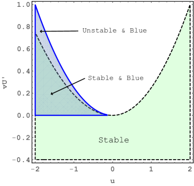
Figure 1: Tensor tilt and stability in the reanalysis of Kamada:2012se . The $u<0$ region was overlooked in the previous analysis. Note in passing that the white region does not satisfy the condition (43).

Since the $\ln X$ terms vanish in $G_{a}$, this case corresponds to the reanalysis of Ref. Kamada:2012se . The tensor tilt and the stability are determined by the two combinations of the functions, $u$ and $vU^{\prime}$. The stability conditions read

$$u+2\sqrt{u^{2}-4vU^{\prime}}>0,$$ (49)

while the tensor tilt depends on the sign of

$${\cal I}=\frac{1}{2}\left(u+\sqrt{u^{2}-4vU^{\prime}}\right).$$ (50)

We plot in Fig. 1 the stable region in the $(u,vU^{\prime})$ plane. It is found that the scalar perturbations are stable and $n_{t}>0$ if

$$u<0,\quad 0<vU^{\prime}<\frac{3}{16}u^{2}.$$ (51)

To realize $n_{t}>0$, it is not necessary to extend the formulation of Kamada:2012se . The region (51) was just overlooked in the previous analysis.

Let us present a simple explicit example whose Lagrangian is given by

$${\cal L}=\frac{M_{\textrm{Pl}}^{2}}{2}R-X-V(\phi)-\frac{\alpha}{\Lambda^{3}}X\Box\phi,$$ (52)

where the potential is approximated by $V=\Lambda^{3}\phi$ in the regime we are interested in. For $0<\alpha<3/16$ the above conditions are satisfied. One obtains a slow-roll inflationary solution,

$$H\simeq\frac{\Lambda^{2}}{(6M_{\textrm{Pl}}^{2}|{\cal I}|)^{1/3}}t^{1/3},\quad\phi\simeq\frac{3M_{\textrm{Pl}}^{2/3}\Lambda}{(6|{\cal I}|)^{2/3}}t^{2/3},$$ (53)

for $t\gg M_{\textrm{Pl}}^{1/2}\Lambda^{-3/2}|{\cal I}|^{1/4}$, where ${\cal I}=(-1+\sqrt{1-4\alpha})/2=\,$const. Note that $H\gg\Lambda^{3/2}M_{\textrm{Pl}}^{-1/2}|{\cal I}|^{-1/4}$ and hence $\Lambda$ must be sufficiently low.

(ii) $v=0$

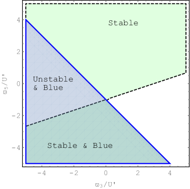
Figure 2: Tensor tilt and stability in $v=0$ models.

In this case, one can easily see how the $\ln X$ terms help to realize $n_{t}>0$. The stability conditions read

$$u>0\quad\textrm{and}\quad\frac{\varpi_{3}}{U^{\prime}+\varpi_{3}+\varpi_{5}}<\frac{3}{4}.$$ (54)

From Eq. (38) and $u>0$ we see that the tensor tilt depends on the sign of $U^{\prime}/(U^{\prime}+\varpi)$. We have a blue tensor spectrum if

$$\frac{U^{\prime}}{U^{\prime}+\varpi_{3}+\varpi_{5}}<0.$$ (55)

Equations (54) and (55) are satisfied simultaneously if

$$\frac{\varpi_{3}}{U^{\prime}}-3\frac{\varpi_{5}}{U^{\prime}}>3\quad\textrm{and}\quad\frac{\varpi_{3}}{U^{\prime}}+\frac{\varpi_{5}}{U^{\prime}}<-1.$$ (56)

Figure 2 summarizes the stability and the tensor tilt in the $(\varpi_{3}/U^{\prime},\varpi_{5}/U^{\prime})$ plane. Note that from the definitions and Eqs. (31) and (39) we see that $\varpi_{3}/U^{\prime}=-3\delta_{3}/(2\epsilon+\delta_{M})$ and $\varpi_{5}/U^{\prime}=-2\delta_{5}/(2\epsilon+\delta_{M})$, and hence we typically have $|\varpi_{3}/U^{\prime}|,|\varpi_{5}/U^{\prime}|\lesssim{\cal O}(1)$.

Let us finally check that the result of Gauss-Bonnet inflation studied in Satoh:2008ck ; Satoh:2010ep ; Koh:2018qcy can be reproduced from our general framework. The Lagrangian considered in Koh:2018qcy is given by

$${\cal L} =\frac{M_{\textrm{Pl}}^{2}}{2}R+X-V(\phi)$$

$$\quad+f(\phi)\left(R^{2}-4R_{\mu\nu}R^{\mu\nu}+R_{\mu\nu\rho\sigma}R^{\mu\nu\rho\sigma}\right).$$ (57)

Ignoring the higher-order terms in the slow-roll approximation, this corresponds to

$$G_{2}=-V+X,\quad G_{3}=0,\quad G_{4}=\frac{M_{\textrm{Pl}}^{2}}{2},$$

$$G_{5}=-4f^{\prime}\ln X,$$ (58)

and hence

$$u=1,\quad v=0,\quad U^{\prime}=V^{\prime},\quad\varpi=\varpi_{5}=-\frac{8}{3}\frac{V^{2}f^{\prime}}{M_{\textrm{Pl}}^{4}}.$$ (59)

It follows from Eq. (56) that stable inflation with $n_{t}>0$ is realized if

$$\frac{\varpi_{5}}{U^{\prime}}<-1\;\;\;\Leftrightarrow\;\;\;\frac{f^{\prime}}{M_{\textrm{Pl}}^{4}}\frac{V^{2}}{V^{\prime}}>\frac{3}{8}.$$ (60)

This reproduces the result of Koh:2018qcy .

The expression for the scalar spectral index can also be reproduced. Using Eq. (30), we obtain $\dot{\phi}^{2}=M_{\textrm{Pl}}^{2}H^{2}(2\epsilon-\delta_{5})$, and hence ${\cal F}=M_{\textrm{Pl}}^{2}(\epsilon-\delta_{5}/2)$. This, together with Eq. (21), leads to

$$n_{s}-1=-2\epsilon-\frac{(2\epsilon-\delta_{5})\dot{}}{(2\epsilon-\delta_{5})H},$$ (61)

which agrees with the result of Koh:2018qcy . In our notation, this can also be written in a simpler way as $n_{s}-1=-4\epsilon+2\eta$. (See Ref. Wu:2017joj for a higher-order calculation of the power spectra in Gauss-Bonnet inflation.)

We have thus successfully extended the work of Kamada:2012se to include Gauss-Bonnet inflation as a specific case. It should be emphasized that our framework not only contains Gauss-Bonnet inflation but also covers a model space of potential-driven slow-roll inflation which has not been explored before.

V Conclusions

In this paper, we have explored the possibility of generating primordial gravitational waves with a positive tilt, $n_{t}>0$, from potential-driven slow-roll inflation. In a canonical inflationary setup this is obviously impossible. While a blue-tilted gravitational wave spectrum can certainly be obtained in kinetically driven G-inflation Kobayashi:2010cm and other more or less radical models Gruzinov:2004ty ; Endlich:2012pz ; Cannone:2014uqa ; Bartolo:2015qvr ; Ricciardone:2016lym ; Fujita:2018ehq ; Ashoorioon:2014nta , it has been claimed in Kamada:2012se that one always has $n_{t}<0$ in generic potential-driven slow-roll inflation constructed within the Horndeski framework Horndeski:1974wa ; Deffayet:2011gz ; Kobayashi:2011nu . It was pointed out, however, that the tensor tilt can indeed be positive in potential-driven slow-roll inflation with the Gauss-Bonnet term Satoh:2008ck ; Satoh:2010ep ; Koh:2018qcy . Since the nonminimal coupling to the Gauss-Bonnet term is a (nontrivial) specific case of the Horndeski Lagrangian, this result implies that the validity of the statement of Kamada:2012se is questionable. In this work, we have therefore extended the formulation of Kamada:2012se in two ways. First, the Taylor-expanded form of the functions in the Horndeski Lagrangian assumed in Kamada:2012se fails to reproduce inflation with the Gauss-Bonnet term and so we have included new terms that are still allowed within the Horndeski framework and help to recover the Gauss-Bonnet term as a specific case. Second, we have reconsidered the validity of the inequality assumed in Kamada:2012se and found that it is in fact too strong. We have shown that a blue gravitational wave spectrum can be obtained even in potential-dominated slow-roll inflation if one relaxes at least either of these two assumptions. We have thus enlarged a possible model space of slow-roll inflation with observationally interesting predictions.

Appendix A The Einstein frame

In this appendix, we discuss the frame (in)dependence of our main result.

One can move to the Einstein frame for the tensor modes by performing a conformal transformation,

$$g_{\mu\nu}\to\tilde{g}_{\mu\nu}=\Omega^{2}(\phi)g_{\mu\nu},\quad\Omega=\frac{\sqrt{2g_{4}}}{M_{\textrm{Pl}}}.$$ (62)

The time coordinate and the scale factor in the Einstein frame is given by

$$\textrm{d}\tilde{t}=\Omega(\phi(t))\textrm{d}t,\quad\tilde{a}(\tilde{t})=\Omega(\phi(t))a(t).$$ (63)

The Hubble parameter in the Einstein frame is obtained as

$$\tilde{H}=\frac{\textrm{d}\ln\tilde{a}}{\textrm{d}\tilde{t}}=\frac{H}{\Omega}\left(1+\frac{\delta_{M}}{2}\right)\simeq\frac{H}{\Omega}.$$ (64)

In terms of the tilde variables, the quadratic action for the tensor perturbations (11) is expressed as

$$\tilde{S}^{(2)}_{h}=\frac{M_{\textrm{Pl}}^{2}}{8}\int\textrm{d}\tilde{t}\textrm{d}^{3}x\,\tilde{a}^{3}\left[(\partial_{\tilde{t}}h_{ij})^{2}-\tilde{a}^{-2}(\partial_{k}h_{ij})^{2}\right],$$ (65)

and hence is of the standard form Creminelli:2014wna . The power spectrum in the Einstein frame is thus of the standard form,

$$\tilde{\cal P}_{h}=\frac{2}{\pi^{2}}\frac{\tilde{H}^{2}}{M_{\textrm{Pl}}^{2}}.$$ (66)

From Eqs. (62) and (64), we see that this coincides with the Jordan frame result (12). Obviously, the spectral index in the Einstein frame coincides with that in the Jordan frame,

$$\tilde{n}_{t}=-2\tilde{\epsilon}\simeq-2\epsilon-\delta_{M}=n_{t}.$$ (67)

This in particular means that, in order to have $\tilde{n}_{t}>0$, the null energy condition must be violated in the Einstein frame Creminelli:2014wna . Note, however, that the conformal transformation (62) preserves the essential nonstandard structure of the scalar sector rather than leads to its standard form. Therefore, one may still have stable inflation models with $\tilde{n}_{t}>0$.

To see this, let us define

$$\tilde{V}=\frac{V}{\Omega^{4}},\quad\tilde{u}=\Omega^{2}u,\quad\tilde{v}=\Omega^{6}v,\quad\tilde{\varpi}_{3,5}=\frac{\varpi_{3,5}}{\Omega^{2}}.$$ (68)

and make the field redefinition via

$$\textrm{d}\varphi=\frac{\textrm{d}\phi}{\Omega^{2}}.$$ (69)

The background equations in terms of the tilde variables read

$$3M_{\textrm{Pl}}^{2}\tilde{H}^{2} \simeq\tilde{V},$$ (70)

$$-2M_{\textrm{Pl}}^{2}\dot{\tilde{H}} \simeq\dot{\varphi}^{2}\tilde{\cal I},$$ (71)

$$3\tilde{H}\dot{\varphi}\tilde{\cal I} \simeq-\frac{\textrm{d}\tilde{V}}{\textrm{d}\varphi},$$ (72)

where

$$\tilde{\cal I}:=\tilde{u}+3\tilde{v}\tilde{H}\dot{\varphi}+\frac{\tilde{\varpi}_{3}+\tilde{\varpi}_{5}}{3\tilde{H}\dot{\varphi}}=\Omega^{2}{\cal I},$$ (73)

and a dot now stands for differentiation with respect to $\tilde{t}$. The information of the nonstandard background evolution is encoded in $\tilde{\cal I}$. Similarly, the quadratic action for the curvature perturbation in terms of the tilde variables is given by

$$\tilde{S}_{\zeta}^{(2)}=\int\textrm{d}\tilde{t}\textrm{d}^{3}x\,\tilde{a}^{3}\frac{\tilde{\cal F}}{\tilde{c}_{s}^{2}}\left[\dot{\zeta}^{2}-\tilde{a}^{-2}\tilde{c}_{s}^{2}(\partial\zeta)^{2}\right],$$ (74)

where

$$\tilde{\cal F} =\frac{\dot{\varphi}^{2}}{2\tilde{H}^{2}}\left(\tilde{u}+4\tilde{v}\tilde{H}\dot{\varphi}+\frac{4\tilde{\varpi}_{3}}{9\tilde{H}\dot{\varphi}}\right)=\frac{{\cal F}}{\Omega^{2}},$$ (75)

$$\tilde{c}_{s}^{2} =\frac{\tilde{u}+4\tilde{v}\tilde{H}\dot{\varphi}+4\tilde{\varpi}_{3}/9\tilde{H}\dot{\varphi}}{\tilde{u}+6\tilde{v}\tilde{H}\dot{\varphi}}=c_{s}^{2}.$$ (76)

With Eq. (64), this clearly shows that the stability and observables are frame-independent.

References

- (1) A. H. Guth, The Inflationary Universe: A Possible Solution to the Horizon and Flatness Problems, Phys. Rev. D23 (1981) 347.
- (2) A. A. Starobinsky, A New Type of Isotropic Cosmological Models Without Singularity, Phys. Lett. B91 (1980) 99.
- (3) K. Sato, First Order Phase Transition of a Vacuum and Expansion of the Universe, Mon. Not. Roy. Astron. Soc. 195 (1981) 467.
- (4) T. Kobayashi, M. Yamaguchi and J. Yokoyama, Generalized G-inflation: Inflation with the most general second-order field equations, Prog. Theor. Phys. 126 (2011) 511 [1105.5723].
- (5) G. W. Horndeski, Second-order scalar-tensor field equations in a four-dimensional space, Int. J. Theor. Phys. 10 (1974) 363.
- (6) C. Deffayet, X. Gao, D. A. Steer and G. Zahariade, From k-essence to generalised Galileons, Phys. Rev. D84 (2011) 064039 [1103.3260].
- (7) T. Kobayashi, Horndeski theory and beyond: a review, Rept. Prog. Phys. 82 (2019) 086901 [1901.07183].
- (8) K. Kamada, T. Kobayashi, M. Yamaguchi and J. Yokoyama, Higgs G-inflation, Phys. Rev. D83 (2011) 083515 [1012.4238].
- (9) K. Kamada, T. Kobayashi, T. Takahashi, M. Yamaguchi and J. Yokoyama, Generalized Higgs inflation, Phys. Rev. D86 (2012) 023504 [1203.4059].
- (10) T. Kobayashi, M. Yamaguchi and J. Yokoyama, G-inflation: Inflation driven by the Galileon field, Phys. Rev. Lett. 105 (2010) 231302 [1008.0603].
- (11) Y.-F. Cai, J.-O. Gong, S. Pi, E. N. Saridakis and S.-Y. Wu, On the possibility of blue tensor spectrum within single field inflation, Nucl. Phys. B900 (2015) 517 [1412.7241].
- (12) Y. Cai, Y.-T. Wang and Y.-S. Piao, Is there an effect of a nontrivial during inflation?, Phys. Rev. D93 (2016) 063005 [1510.08716].
- (13) Y. Cai, Y.-T. Wang and Y.-S. Piao, Propagating speed of primordial gravitational waves and inflation, Phys. Rev. D94 (2016) 043002 [1602.05431].
- (14) A. Gruzinov, Elastic inflation, Phys. Rev. D70 (2004) 063518 [astro-ph/0404548].
- (15) S. Endlich, A. Nicolis and J. Wang, Solid Inflation, JCAP 1310 (2013) 011 [1210.0569].
- (16) D. Cannone, G. Tasinato and D. Wands, Generalised tensor fluctuations and inflation, JCAP 1501 (2015) 029 [1409.6568].
- (17) N. Bartolo, D. Cannone, A. Ricciardone and G. Tasinato, Distinctive signatures of space-time diffeomorphism breaking in EFT of inflation, JCAP 1603 (2016) 044 [1511.07414].
- (18) A. Ricciardone and G. Tasinato, Primordial gravitational waves in supersolid inflation, Phys. Rev. D96 (2017) 023508 [1611.04516].
- (19) T. Fujita, S. Kuroyanagi, S. Mizuno and S. Mukohyama, Blue-tilted Primordial Gravitational Waves from Massive Gravity, Phys. Lett. B789 (2019) 215 [1808.02381].
- (20) A. Ashoorioon, K. Dimopoulos, M. M. Sheikh-Jabbari and G. Shiu, Non-Bunch-Davis initial state reconciles chaotic models with BICEP and Planck, Phys. Lett. B737 (2014) 98 [1403.6099].
- (21) M. Satoh and J. Soda, Higher Curvature Corrections to Primordial Fluctuations in Slow-roll Inflation, JCAP 0809 (2008) 019 [0806.4594].
- (22) M. Satoh, Slow-roll Inflation with the Gauss-Bonnet and Chern-Simons Corrections, JCAP 1011 (2010) 024 [1008.2724].
- (23) Z.-K. Guo and D. J. Schwarz, Slow-roll inflation with a Gauss-Bonnet correction, Phys. Rev. D81 (2010) 123520 [1001.1897].
- (24) P.-X. Jiang, J.-W. Hu and Z.-K. Guo, Inflation coupled to a Gauss-Bonnet term, Phys. Rev. D88 (2013) 123508 [1310.5579].
- (25) S. Koh, B.-H. Lee, W. Lee and G. Tumurtushaa, Observational constraints on slow-roll inflation coupled to a Gauss-Bonnet term, Phys. Rev. D90 (2014) 063527 [1404.6096].
- (26) S. Koh, B.-H. Lee and G. Tumurtushaa, Reconstruction of the Scalar Field Potential in Inflationary Models with a Gauss-Bonnet term, Phys. Rev. D95 (2017) 123509 [1610.04360].
- (27) S. Bhattacharjee, D. Maity and R. Mukherjee, Constraining scalar-Gauss-Bonnet Inflation by Reheating, Unitarity and PLANCK, Phys. Rev. D95 (2017) 023514 [1606.00698].
- (28) C. van de Bruck, K. Dimopoulos and C. Longden, Reheating in Gauss-Bonnet-coupled inflation, Phys. Rev. D94 (2016) 023506 [1605.06350].
- (29) K. Nozari and N. Rashidi, Perturbation, non-Gaussianity, and reheating in a Gauss-Bonnet -attractor model, Phys. Rev. D95 (2017) 123518 [1705.02617].
- (30) Q. Wu, T. Zhu and A. Wang, Primordial Spectra of slow-roll inflation at second-order with the Gauss-Bonnet correction, Phys. Rev. D97 (2018) 103502 [1707.08020].
- (31) S. Koh, B.-H. Lee and G. Tumurtushaa, Constraints on the reheating parameters after Gauss-Bonnet inflation from primordial gravitational waves, Phys. Rev. D98 (2018) 103511 [1807.04424].
- (32) S. Chakraborty, T. Paul and S. SenGupta, Inflation driven by Einstein-Gauss-Bonnet gravity, Phys. Rev. D98 (2018) 083539 [1804.03004].
- (33) F. L. Bezrukov and M. Shaposhnikov, The Standard Model Higgs boson as the inflaton, Phys. Lett. B659 (2008) 703 [0710.3755].
- (34) C. Germani and A. Kehagias, New Model of Inflation with Non-minimal Derivative Coupling of Standard Model Higgs Boson to Gravity, Phys. Rev. Lett. 105 (2010) 011302 [1003.2635].
- (35) P. Creminelli, J. Gleyzes, J. Noreña and F. Vernizzi, Resilience of the standard predictions for primordial tensor modes, Phys. Rev. Lett. 113 (2014) 231301 [1407.8439].