Intriguing Properties of Adversarial ML Attacks
in the Problem Space

Abstract

Recent research efforts on adversarial ML have investigated problem-space attacks, focusing on the generation of real evasive objects in domains where, unlike images, there is no clear inverse mapping to the feature space (e.g., software). However, the design, comparison, and real-world implications of problem-space attacks remain underexplored.

This paper makes two major contributions. First, we propose a novel formalization for adversarial ML evasion attacks in the problem-space, which includes the definition of a comprehensive set of constraints on available transformations, preserved semantics, robustness to preprocessing, and plausibility. We shed light on the relationship between feature space and problem space, and we introduce the concept of side-effect features as the by-product of the inverse feature-mapping problem. This enables us to define and prove necessary and sufficient conditions for the existence of problem-space attacks. We further demonstrate the expressive power of our formalization by using it to describe several attacks from related literature across different domains.

Second, building on our formalization, we propose a novel problem-space attack on Android malware that overcomes past limitations. Experiments on a dataset with 170K Android apps from 2017 and 2018 show the practical feasibility of evading a state-of-the-art malware classifier along with its hardened version. Our results demonstrate that “adversarial-malware as a service” is a realistic threat, as we automatically generate thousands of realistic and inconspicuous adversarial applications at scale, where on average it takes only a few minutes to generate an adversarial app. Yet, out of the 1600+ papers on adversarial ML published in the past six years, roughly 40 focus on malware [15]—and many remain only in the feature space.

Our formalization of problem-space attacks paves the way to more principled research in this domain. We responsibly release the code and dataset of our novel attack to other researchers, to encourage future work on defenses in the problem space.

I Introduction

Adversarial ML attacks are being studied extensively in multiple domains [11] and pose a major threat to the large-scale deployment of machine learning solutions in security-critical contexts. This paper focuses on test-time evasion attacks in the so-called problem space, where the challenge lies in modifying real input-space objects that correspond to an adversarial feature vector. The main challenge resides in the inverse feature-mapping problem [47, 46, 58, 32, 12, 13] since in many settings it is not possible to convert a feature vector into a problem-space object because the feature-mapping function is neither invertible nor differentiable. In addition, the modified problem-space object needs to be a valid, inconspicuous member of the considered domain, and robust to non-ML preprocessing. Existing work investigated problem-space attacks on text [3, 43], malicious PDFs [46, 45, 12, 74, 41, 22], Android malware [23, 75], Windows malware [38, 60], NIDS [28, 6, 7, 20], ICS [76], source code attribution [58], malicious Javascript [27], and eyeglass frames [62]. However, while there is a good understanding on how to perform feature-space attacks [16], it is less clear what the requirements are for an attack in the problem space, and how to compare strengths and weaknesses of existing solutions in a principled way.

In this paper, motivated by examples on software, we propose a novel formalization of problem-space attacks, which lays the foundation for identifying key requirements and commonalities among different domains. We identify four major categories of constraints to be defined at design time: which problem-space transformations are available to be performed automatically while looking for an adversarial variant; which object semantics must be preserved between the original and its adversarial variant; which non-ML preprocessing the attack should be robust to (e.g., image compression, code pruning); and how to ensure that the generated object is a plausible member of the input distribution, especially upon manual inspection. We introduce the concept of side-effect features as the by-product of trying to generate a problem-space transformation that perturbs the feature space in a certain direction. This allows us to shed light on the relationships between feature space and problem space: we define and prove necessary and sufficient conditions for the existence of problem-space attacks, and identify two main types of search strategies (gradient-driven and problem-driven) for generating problem-space adversarial objects.

We further use our formalization to describe several interesting attacks proposed in both problem space and feature space. This analysis shows that prior promising problem-space attacks in the malware domain [60, 75, 31] suffer from limitations, especially in terms of semantics and preprocessing robustness. Grosse et al. [31] only add individual features to the Android manifest, which preserves semantics, but can be removed with preprocessing (e.g., by detecting unused permissions); moreover, they are constrained by a maximum feature-space perturbation, which we show is less relevant for problem-space attacks. Rosenberg et al. [60] leave artifacts during the app transformation which are easily detected through lightweight non-ML techniques. Yang et al. [75] may significantly alter the semantics of the program (which may account for the high failure rate observed in their mutated apps), and do not specify which preprocessing techniques they consider. These inspire us to propose, through our formalization, a novel problem-space attack in the Android malware domain that overcomes limitations of existing solutions.

In summary, this paper has two major contributions:

• We propose a novel formalization of problem-space attacks (§ II) which lays the foundation for identifying key requirements and commonalities of different domains, proves necessary and sufficient conditions for problem-space attacks, and allows for the comparison of strengths and weaknesses of prior approaches—where existing strategies for adversarial malware generation are among the weakest in terms of attack robustness. We introduce the concept of side-effect features, which reveals connections between feature space and problem space, and enables principled reasoning about search strategies for problem-space attacks.

• Building on our formalization, we propose a novel problem-space attack in the Android malware domain, which relies on automated software transplantation [10] and overcomes limitations of prior work in terms of semantics and preprocessing robustness (§ III). We experimentally demonstrate (§ IV) on a dataset of 170K apps from 2017-2018 that it is feasible for an attacker to evade a state-of-the-art malware classifier, DREBIN [8], and its hardened version, Sec-SVM [23]. The time required to generate an adversarial example is in the order of minutes, thus demonstrating that the “adversarial-malware as a service” scenario is a realistic threat, and existing defenses are not sufficient.

To foster future research on this topic, we discuss promising defense directions (§ V) and responsibly release the code and data of our novel attack to other researchers via access to a private repository (§ VII).

II Problem-Space Adversarial ML Attacks

We focus on evasion attacks [12, 16, 32], where the adversary modifies objects at test time to induce targeted misclassifications. We provide background from related literature on feature-space attacks (§ II-A), and then introduce a novel formalization of problem-space attacks (§ II-B). Finally, we highlight the main parameters of our formalization by instantiating it on both traditional feature-space and more recent problem-space attacks from related works in several domains (§ II-C). Threat modeling based on attacker knowledge and capability is the same as in related work [11, 65, 19], and is reported in Appendix -B for completeness. To ease readability, Appendix -A reports a symbol table.

II-A Feature-Space Attacks

We remark that all definitions of feature-space attacks (§ II-A) have already been consolidated in related work [11, 16, 23, 31, 66, 33, 21, 44]; we report them for completeness and as a basis for identifying relationships between feature-space and problem-space attacks in the following subsections.

We consider a problem space $\mathcal{Z}$ (also referred to as input space) that contains objects of a considered domain (e.g., images [16], audio [17], programs [58], PDFs [45]). We assume that each object $z\in\mathcal{Z}$ is associated with a ground-truth label $y\in\mathcal{Y}$, where $\mathcal{Y}$ is the space of possible labels. Machine learning algorithms mostly work on numerical vector data [14], hence the objects in $\mathcal{Z}$ must be transformed into a suitable format for ML processing.

Definition 1 (Feature Mapping).

A feature mapping is a function $\varphi:\mathcal{Z}\longrightarrow\mathcal{X}\subseteq\mathbb{R}^{n}$ that, given a problem-space object $z\in\mathcal{Z}$, generates an $n$-dimensional feature vector $\bm{x}\in\mathcal{X}$, such that $\varphi(z)=\bm{x}$. This also includes implicit/latent mappings, where the features are not observable in input but are instead implicitly computed by the model (e.g., deep learning [29]).

Definition 2 (Discriminant Function).

Given an $m$-class machine learning classifier $g:\mathcal{X}\longrightarrow\mathcal{Y}$, a discriminant function $h:\mathcal{X}\times\mathcal{Y}\longrightarrow\mathbb{R}$ outputs a real number $h(\bm{x},i)$, for which we use the shorthand $h_{i}(\bm{x})$, that represents the fitness of object $\bm{x}$ to class $i\in\mathcal{Y}$. Higher outputs of the discriminant function $h_{i}$ represent better fitness to class $i$. In particular, the predicted label of an object $\bm{x}$ is $g(\bm{x})=\hat{y}=\arg\max_{i\in\mathcal{Y}}h_{i}(\bm{x})$.

The purpose of a targeted feature-space attack is to modify an object $\bm{x}\in\mathcal{X}$ with assigned label $y\in\mathcal{Y}$ to an object $\bm{x}^{\prime}$ that is classified to a target class $t\in\mathcal{Y}$, $t\neq y$ (i.e., to modify $\bm{x}$ so that it is misclassified as a target class $t$). The attacker can identify a perturbation $\bm{\delta}$ to modify $\bm{x}$ so that $g(\bm{x}+\bm{\delta})=t$ by optimizing a carefully-crafted attack objective function. We refer to the definition of attack objective function in Carlini and Wagner [16] and in Biggio and Roli [11], which takes into account high-confidence attacks and multi-class settings.

Definition 3 (Attack Objective Function).

Given an object $\bm{x}\in\mathcal{X}$ and a target label $t\in\mathcal{Y}$, an attack objective function $f:\mathcal{X}\times\mathcal{Y}\longrightarrow\mathbb{R}$ is defined as follows:

$$f(\bm{x},t)=\max_{i\neq t}\{h_{i}(\bm{x})\}-h_{t}(\bm{x})\,,$$ (1)

for which we use the shorthand $f_{t}(\bm{x})$. Generally, $\bm{x}$ is classified as a member of $t$ if and only if $f_{t}(\bm{x})<0$. An adversary can also enforce a desired attack confidence $\kappa\in\mathbb{R}$ such that the attack is considered successful if and only if $f_{t}(\bm{x})<-\kappa$.

The intuition is to minimize $f_{t}$ by modifying $\bm{x}$ in directions that follow the negative gradient of $f_{t}$, i.e., to get $\bm{x}$ closer to the target class $t$.

In addition to the attack objective function, a considered problem-space domain may also come with constraints on the modification of the feature vectors. For example, in the image domain the value of pixels must be bounded between 0 and 255 [16]; in software, some features in $\bm{x}$ may only be added but not removed (e.g., API calls [23]).

Definition 4 (Feature-Space Constraints).

We define $\Omega$ as the set of feature-space constraints, i.e., a set of constraints on the possible feature-space modifications. The set $\Omega$ reflects the requirements of realistic problem-space objects. Given an object $\bm{x}\in\mathcal{X}$, any modification of its feature values can be represented as a perturbation vector $\bm{\delta}\in\mathbb{R}^{n}$; if $\bm{\delta}$ satisfies $\Omega$, we borrow notation from model theory [72] and write $\bm{\delta}\models\Omega$.

As examples of feature-space constraints, in the image domain [e.g., 16, 11] the perturbation $\bm{\delta}$ is subject to an upper bound based on $l_{p}$ norms ($||\bm{\delta}||_{p}\leq\delta_{max}$), to preserve similarity to the original object; in the software domain [e.g., 23, 31], only some features of $\bm{x}$ may be modified, such that $\bm{\delta}_{lb}\preceq\bm{\delta}\preceq\bm{\delta}_{ub}$ (where $\bm{\delta}_{1}\preceq\bm{\delta}_{2}$ implies that each element of $\bm{\delta}_{1}$ is $\leq$ the corresponding i-th element in $\bm{\delta}_{2}$).

We can now formalize the traditional feature-space attack as in related work [16, 12, 23, 11, 52].

Definition 5 (Feature-Space Attack).

Given a machine learning classifier $g$, an object $\bm{x}\in\mathcal{X}$ with label $y\in\mathcal{Y}$, and a target label $t\in\mathcal{Y},\,t\neq y$, the adversary aims to identify a perturbation vector $\bm{\delta}\in\mathbb{R}^{n}$ such that $g(\bm{x}+\bm{\delta})=t$. The desired perturbation can be achieved by solving the following optimization problem:

$$\bm{\delta}^{*}=\arg\min_{\bm{\delta}\in\mathbb{R}^{n}}\quad f_{t}(\bm{x}+\bm{\delta})$$ (2)

subject to: $$\bm{\delta}\models\Omega\,.$$ (3)

A feature-space attack is successful if $f_{t}(\bm{x}+\bm{\delta}^{*})<0$ (or less than $-\kappa$, if a desired attack confidence is enforced).

Without loss of generality, we observe that the feature-space attacks definition can be extended to ensure that the adversarial example is closer to the training data points (e.g., through the tuning of a parameter $\lambda$ that penalizes adversarial examples generated in low density regions, as in the mimicry attacks of Biggio et al. [12]).

II-B Problem-Space Attacks

This section presents a novel formalization of problem-space attacks and introduces insights into the relationship between feature space and problem space.

Inverse Feature-Mapping Problem. The major challenge that complicates (and, in most cases, prevents) the direct applicability of gradient-driven feature-space attacks to find problem-space adversarial examples is the so-called inverse feature-mapping problem [47, 46, 58, 32, 12, 13]. As an extension, Quiring et al. [58] discuss the feature-problem space dilemma, which highlights the difficulty of moving in both directions: from feature space to problem space, and from problem space to feature space. In most cases, the feature mapping function $\varphi$ is not bijective, i.e., not injective and not surjective. This means that given $z\in\mathcal{Z}$ with features $\bm{x}$, and a feature-space perturbation $\bm{\delta}^{*}$, there is no one-to-one mapping that allows going from $\bm{x}+\bm{\delta}^{*}$ to an adversarial problem-space object $z^{\prime}$. Nevertheless, there are two additional scenarios. If $\varphi$ is not invertible but is differentiable, then it is possible to backpropagate the gradient of $f_{t}(\bm{x})$ from $\mathcal{X}$ to $\mathcal{Z}$ to derive how the input can be changed in order to follow the negative gradient (e.g., to know which input pixels to perturbate to follow the gradient in the deep-learning latent feature space). If $\varphi$ is not invertible and not differentiable, then the challenge is to find a way to map the adversarial feature vector $\bm{x}^{\prime}\in\mathcal{X}$ to an adversarial object $z^{\prime}\in\mathcal{Z}$, by applying a transformation to $z$ in order to produce $z^{\prime}$ such that $\varphi(z^{\prime})$ is “as close as possible” to $\bm{x}^{\prime}$; i.e., to follow the gradient towards the transformation that most likely leads to a successful evasion [38]. In problem-space settings such as software, the function $\varphi$ is typically not invertible and not differentiable, so the search for transforming $z$ to perform the attack cannot be purely gradient-based.

In this section, we consider the general case in which the feature mapping $\varphi$ is not differentiable and not invertible (i.e., the most challenging setting), and we refer to this context to formalize problem-space evasion attacks.

First, we define a problem-space transformation operator through which we can alter problem-space objects. Due to their generality, we adapt the code transformation definitions from the compiler engineering literature [1, 58] to formalize general problem-space transformations.

Definition 6 (Problem-Space Transformation).

A problem-space transformation $T:\mathcal{Z}\longrightarrow\mathcal{Z}$ takes a problem-space object $z\in\mathcal{Z}$ as input and modifies it to $z^{\prime}\in\mathcal{Z}$. We refer to the following notation: $T(z)=z^{\prime}$.

The possible problem-space transformations are either addition, removal, or modification (i.e., combination of addition and removal). In the case of programs, obfuscation is a special case of modification.

Definition 7 (Transformation Sequence).

A transformation sequence $\text{\bf T}=T_{n}\circ T_{n-1}\circ\dots\circ T_{1}$ is the subsequent application of problem-space transformations to an object $z\in\mathcal{Z}$.

Intuitively, given a problem-space object $z\in\mathcal{Z}$ with label $y\in\mathcal{Y}$, the purpose of the adversary is to find a transformation sequence T such that the transformed object $\text{\bf T}(z)$ is classified into any target class $t$ chosen by the adversary ($t\in\mathcal{Y}$, $t\neq y$). One way to achieve such a transformation is to first compute a feature-space perturbation $\bm{\delta}^{*}$, and then modify the problem-space object $z$ so that features corresponding to $\bm{\delta}^{*}$ are carefully altered. However, in the general case where the feature mapping $\varphi$ is neither invertible nor differentiable, the adversary must perform a search in the problem-space that approximately follows the negative gradient in the feature space. However, this search is not unconstrained, because the adversarial problem-space object $\text{\bf T}(z)$ must be realistic.

Problem-Space Constraints. Given a problem-space object $z\in\mathcal{Z}$, a transformation sequence T must lead to an object $z^{\prime}=\text{\bf T}(z)$ that is valid and realistic. To express this formally, we identify four main types of constraints common to any problem-space attack:

1. Available transformations, which describe which modifications can be performed in the problem-space by the attacker (e.g., only addition and not removal).

2. Preserved semantics, the semantics to be preserved while mutating $z$ to $z^{\prime}$, with respect to specific feature abstractions which the attacker aims to be resilient against (e.g., in programs, the transformed object may need to produce the same dynamic call traces). Semantics may also be preserved by construction [e.g., 58].

3. Plausibility (or Inconspicuousness), which describes which (qualitative) properties must be preserved in mutating $z$ to $z^{\prime}$, so that $z$ appears realistic upon manual inspection. For example, often an adversarial image must look like a valid image from the training distribution [16]; a program’s source code must look manually written and not artificially or inconsistently altered [58]. In the general case, verification of plausibility may be hard to automate and may require human analysis.

4. Robustness to preprocessing, which determines which non-ML techniques could disrupt the attack (e.g., filtering in images, dead code removal in programs).

These constraints have been sparsely mentioned in prior literature [12, 58, 74, 11], but have never been identified together as a set for problem-space attacks. When designing a novel problem-space attack, it is fundamental to explicitly define these four types of constraints, to clarify strengths and weaknesses. While we believe that this framework captures all nuances of the current state-of-the-art for a thorough evaluation and comparison, we welcome future research that uses this as a foundation to identify new constraints.

We now introduce formal definitions for the constraints. First, similarly to [23, 11], we define the space of available transformations.

Definition 8 (Available Transformations).

We define $\mathcal{T}$ as the space of available transformations, which determines which types of automated problem-space transformations $T$ the attacker can perform. In general, it determines if and how the attacker can add, remove, or edit parts of the original object $z\in\mathcal{Z}$ to obtain a new object $z^{\prime}\in\mathcal{Z}$. We write $\text{\bf T}\in\mathcal{T}$ if a transformation sequence consists of available transformations.

For example, the pixels of an image may be modified only if they remain within the range of integers 0 to 255 [e.g., 16]; in programs, an adversary may only add valid no-op API calls to ensure that modifications preserve functionality [e.g., 60].

Moreover, the attacker needs to ensure that some semantics are preserved during the transformation of $z$, according to some feature abstractions. Semantic equivalence is known to be generally undecidable [10, 58]; hence, as in [10], we formalize semantic equivalence through testing, by borrowing notation from denotational semantics [57].

Definition 9 (Preserved Semantics).

Let us consider two problem-space objects $z$ and $z^{\prime}=\text{\bf T}(z)$, and a suite of automated tests $\Upsilon$ to verify preserved semantics. We define $z$ and $z^{\prime}$ to be semantically equivalent with respect to $\Upsilon$ if they satisfy all its tests $\tau\in\Upsilon$, where $\tau:\mathcal{Z}\times\mathcal{Z}\longrightarrow\mathbb{B}$. In particular, we denote semantics equivalence with respect to a test suite $\Upsilon$ as follows:

$$\llbracket z\rrbracket^{\tau}=\llbracket z^{\prime}\rrbracket^{\tau},\,\forall\tau\in\Upsilon\,,$$ (4)

where $\llbracket z\rrbracket^{\tau}$ denotes the semantics of $z$ induced during test $\tau$.

Informally, $\Upsilon$ consists of tests that are aimed at evaluating whether $z$ and $z^{\prime}$ (or parts of them) lead to the same abstract representations in a certain feature space. In other words, the tests in $\Upsilon$ model preserved semantics. For example, in programs a typical test aims to verify that malicious functionality is preserved; this is done through tests where, given a certain test input, the program produces exactly the same output [10]. Additionally, the attacker may want to ensure that an adversarial program ($z^{\prime}$) leads to the same instruction trace as its benign version ($z$)—so as not to raise suspicion in feature abstractions derived from dynamic analysis.

Plausibility is more subjective than semantic equivalence, but in many scenarios it is critical that an adversarial object is inconspicuous when manually audited by a human. In order to be plausible, an analyst must believe that the adversarial object is a valid member of the problem-space distribution.

Definition 10 (Plausibility).

We define $\Pi$ as the set of (typically) manual tests to verify plausibility. We say $z$ looks like a valid member of the data distribution to a human being if it satisfies all tests $\pi\in\Pi$, where $\pi:\mathcal{Z}\longrightarrow\mathbb{B}$.

Plausibility is often hard to verify automatically; previous work has often relied on user studies with domain experts to judge the plausibility of the generated objects (e.g., program plausibility in [58], realistic eyeglass frames in [62]). Plausibility in software-related domains may also be enforced by construction during the transformation process, e.g., by relying on automated software transplantation [10, 75].

In addition to semantic equivalence and plausibility, the adversarial problem-space objects need to ensure they are robust to non-ML automated preprocessing techniques that could alter properties on which the adversarial attack depends, thus compromising the attack.

Definition 11 (Robustness to Preprocessing).

We define $\Lambda$ as the set of preprocessing operators an object $z^{\prime}=\text{\bf T}(z)$ should be resilient to. We say $z^{\prime}$ is robust to preprocessing if $\text{\bf A}(\text{\bf T}(z))=\text{\bf T}(z)$ for all $\text{\bf A}\in\Lambda$, where $\text{\bf A}:\mathcal{Z}\longrightarrow\mathcal{Z}$ simulates an expected preprocessing.

Examples of preprocessing operators in $\Lambda$ include compression to remove pixel artifacts (in images), filters to remove noise (in audio), and program analysis to remove dead or redundant code (in programs).

Properties affected by preprocessing are often related to fragile and spurious features learned by the target classifier. While taking advantage of such features may be necessary to demonstrate the weaknesses of the target model, an attacker should be aware that these brittle features are usually the first to change when a model is improved. Given this, a stronger attack is one that does not rely on them.

As a concrete example, in an attack on authorship attribution, Quiring et al. [58] purposefully omit layout features (such as the use of spaces vs. tabs) which are trivial to change. Additionally, Xu et al. [74] discovered the presence of font objects was a critical (but erroneously discriminative) feature following their problem-space attack on PDF malware. These are features that are cheap for an attacker to abuse but can be easily removed by the application of some preprocessing. As a defender, investigation of this constraint will help identify features that are weak to adversarial attacks. Note that knowledge of preprocessing can also be exploited by the attacker (e.g., in scaling attacks [73]).

We can now define a fundamental set of problem-space constraint elements from the previous definitions.

Definition 12 (Problem-Space Constraints).

We define the problem-space constraints $\Gamma=\{\mathcal{T},\Upsilon,\Pi,\Lambda\}$ as the set of all constraints satisfying $\mathcal{T},\Upsilon,\Pi,\Lambda$. We write $\text{\bf T}(z)\models\Gamma$ if a transformation sequence applied to object $z\in\mathcal{Z}$ satisfies all the problem-space constraints, and we refer to this as a valid transformation sequence. The problem-space constraints $\Gamma$ determine the feature-space constraints $\Omega$, and we denote this relationship as $\Gamma\vdash\Omega$ (i.e., $\Gamma$ determines $\Omega$); with a slight abuse of notation, we can also write that $\Omega\subseteq\Gamma$, because some constraints may be specific to the problem space (e.g., program size similar to that of benign applications) and may not be possible to enforce in the feature space $\mathcal{X}$.

Side-Effect Features. Satisfying the problem-space constraints $\Gamma$ further complicates the inverse feature mapping, as $\Gamma$ is a superset of $\Omega$. Moreover, enforcing $\Gamma$ may require substantially altering an object $z$ to ensure satisfaction of all constraints during mutations. Let us focus on an example in the software domain, so that $z$ is a program with features $\bm{x}$; if we want to transform $z$ to $z^{\prime}$ such that $\varphi(z^{\prime})=\bm{x}+\bm{\delta}$, we may want to add to $z$ a program $o$ where $\varphi(o)=\bm{\delta}$. However, the union of $z$ and $o$ may have features different from $\bm{x}+\bm{\delta}$, because other consolidation operations are required (e.g., name deduplication, class declarations, resource name normalization)—which cannot be feasibly computed in advance for each possible object in $\mathcal{Z}$. Hence, after modifying $z$ in an attempt to obtain a problem-space object $z^{\prime}$ with certain features (e.g., close to $\bm{x}+\bm{\delta}$), the attacker-modified object may have some additional features that are not related to the intended transformation (e.g., adding an API which maps to a feature in $\bm{\delta}$), but are required to satisfy all the problem-space constraints in $\Gamma$ (e.g., inserting valid parameters for the API call, and importing dependencies for its invocation). We call side-effect features $\bm{\eta}$ the features that are altered in $z^{\prime}=\text{\bf T}(z)$ specifically for the satisfaction of problem-space constraints. We observe that these features do not follow any particular direction of the gradient, and hence they could have both a positive or negative impact on the classification score.

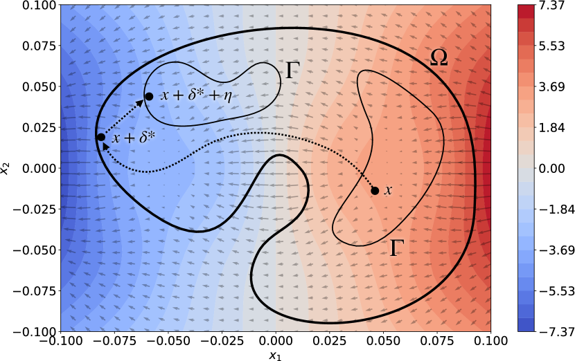
Figure 1: Example of projection of the feature-space attack vector $\bm{x}+\bm{\delta}^{*}$ in the feasible problem space, resulting in side-effect features $\bm{\eta}$. The background displays the value of the discriminant function $h(\bm{x})$, where negative values indicate the target class of the evasion attack. Small arrows represent directions of the negative gradient. The thick solid line represents the feasible feature space determined by $\Omega$, and the thin solid line that determined by $\Gamma$ (which is more restrictive). The dotted arrow represents the gradient-based attack $\bm{x}+\bm{\delta}^{*}$ derived from $\bm{x}$, which is then projected into $\bm{x}+\bm{\delta}^{*}+\bm{\eta}$ to fit into the feasible problem space.

Analogy with Projection. Figure 1 presents an analogy between side-effect features $\bm{\eta}$ and the notion of projection in numerical optimization [14], which helps explain the nature and impact of $\bm{\eta}$ in problem-space attacks. The right half corresponds to higher values of a discriminant function $h(\bm{x})$ and the left half to lower values. The vertical central curve (where the heatmap value is equal to zero) represents the decision boundary: objects on the left-half are classified as negative (e.g., benign), and objects on the right-half as positive (e.g., malicious). The goal of the adversary is to conduct a maximum confidence attack that has an object misclassified as the negative class. The thick solid line represents the feasible feature space determined by constraints $\Omega$, and the thin solid line the feasible problem space determined by $\Gamma$ (which corresponds to two unconnected areas). We assume that the initial object $\bm{x}\in\mathcal{X}$ is always within the feasible problem space. In this example, the attacker first conducts a gradient-based attack in the feature space on object $\bm{x}$, which results in a feature vector $\bm{x}+\bm{\delta}^{*}$, which is classified as negative with high-confidence. However, this point is not in the feasibility space of constraints $\Gamma$, which is more restrictive than that of $\Omega$. Hence, the attacker needs to find a projection that maps $\bm{x}+\bm{\delta}^{*}$ back to the feasible problem-space regions, which leads to the addition of a side-effect feature vector $\bm{\eta}$.

Definition 13 (Side-Effect Feature Vector).

We define $\bm{\eta}$ as the side-effect feature vector that results from enforcing $\Gamma$ while choosing a sequence of transformations T such that $\text{\bf T}(z)\models\Gamma$. In other words, $\bm{\eta}$ are the features derived from the projection of a feature-space attack onto a feasibility region that satisfies problem-space constraints $\Gamma$.

We observe that in settings where the feature mapping $\varphi$ is neither differentiable nor invertible, and where the problem-space representation is very different from the feature-space representation (e.g., unlike in images or audio), it is generally infeasible or impossible to compute the exact impact of side-effect features on the objective function in advance—because the set of problem-space constraints $\Gamma$ cannot be expressed analytically in closed-form. Hence the attacker needs to find a transformation sequence T such that $\varphi(\text{\bf T}(z))=\varphi(z^{\prime})$ is within the feasibility region of problem-space constraints $\Gamma$.

It is relevant to observe that, in the general case, if an object $z_{o}$ is added to (or removed from) two different objects $z_{1}$ and $z_{2}$, it is possible that the resulting side-effect feature vectors $\bm{\eta}_{1}$ and $\bm{\eta}_{2}$ are different (e.g., in the software domain [58]).

Considerations on Attack Confidence. There are some important characteristics of the impact of the side-effect features $\bm{\eta}$ on the attack objective function. If the attacker performs a maximum-confidence attack in the feature space under constraints $\Omega$, then the confidence of the problem-space attack will always be lower or equal than the one in the feature-space attack. This is intuitively represented in Figure 1, where the point is moved to the maximum-confidence attack area within $\Omega$, and the attack confidence is reduced after projection to the feasibility space of the problem space, induced by $\Gamma$. In general, the confidence of the feature- and problem-space attacks could be equal, depending on the constraints $\Omega$ and $\Gamma$, and on the shape of the discriminant function $h$, which is also not necessarily convex (e.g., in deep learning [29]). In the case of low-confidence feature-space attacks, projecting into the problem-space feasibility constraint may result in a positive or negative impact (not known a priori) on the value of the discriminant function. This can be seen from Figure 1, where the object $\bm{x}+\bm{\delta}^{*}$ would be found close to the center of the plot, where $h(\bm{x})=0$.

Problem-Space Attack. We now have all the components required to formalize a problem-space attack.

Definition 14 (Problem-Space Attack).

We define a problem-space attack as the problem of finding the sequence of valid transformations T for which the object $z\in\mathcal{Z}$ with label $y\in\mathcal{Y}$ is misclassified to a target class $t\in\mathcal{Y}$ as follows:

$$\text{argmin}_{\text{\bf T}\in\mathcal{T}}\quad f_{t}(\varphi(\text{\bf T}(z)))=f_{t}(\bm{x}+\bm{\delta}^{*}+\bm{\eta})$$ (5)

subject to: $$\llbracket z\rrbracket^{\tau}=\llbracket\text{\bf T}(z)\rrbracket^{\tau},\quad\forall\tau\in\Upsilon$$ (6)

$$\pi(\text{\bf T}(z))=1,\quad\forall\pi\in\Pi$$ (7)

$${\text{\bf A}(\text{\bf T}(z))=\text{\bf T}(z),\quad\forall\text{\bf A}\in\Lambda}$$ (8)

where $\bm{\eta}$ is a side-effect feature vector that separates the feature vector generated by $\text{\bf T}(z)$ from the theoretical feature-space attack $\bm{x}+\bm{\delta}^{*}$ (under constraints $\Omega$). An equivalent, more compact, formulation is as follows:

$$\text{argmin}_{\text{\bf T}\in\mathcal{T}}\quad f_{t}(\varphi(\text{\bf T}(z)))=f_{t}(\bm{x}+\bm{\delta}^{*}+\bm{\eta})$$ (9)

subject to: $$\text{\bf T}(z)\models\Gamma\,.$$ (10)

Search Strategy. The typical search strategy for adversarial perturbations in feature-space attacks is based on following the negative gradient of the objective function through some numerical optimization algorithm, such as stochastic gradient descent [11, 16, 17]. However, it is not possible to directly apply gradient descent in the general case of problem-space attacks, when the feature space is not invertible nor differentiable [58, 11]; and it is even more complicated if a transformation sequence T produces side-effect features $\bm{\eta}\neq\bm{0}$. In the problem space, we identify two main types of search strategy: problem-driven and gradient-driven. In the problem-driven approach, the search of the optimal T proceeds heuristically by beginning with random mutations of the object $z$, and then learning from experience how to appropriately mutate it further in order to misclassify it to the target class (e.g., using Genetic Programming [74] or variants of Monte Carlo tree search [58]). This approach iteratively uses local approximations of the negative gradient to mutate the objects. The gradient-driven approach attempts to identify mutations that follow the negative gradient by relying on an approximate inverse feature mapping (e.g., in PDF malware [46], in Android malware [75]). If a search strategy equally makes extensive use of both problem-driven and gradient-driven methods, we call it a hybrid strategy. We note that search strategies may have different trade-offs in terms of effectiveness and costs, depending on the time and resources they require. While there are some promising avenues in this challenging but important line of research [39], it warrants further investigation in future work.

Feature-space attacks can still give us some useful information: before searching for a problem-space attack, we can verify whether a feature-space attack exists, which is a necessary condition for realizing the problem-space attack.

Theorem 1 (Necessary Condition for Problem-Space Attacks).

Given a problem-space object $z\in\mathcal{Z}$ of class $y\in\mathcal{Y}$, with features $\varphi(z)=\bm{x}$, and a target class $t\in\mathcal{Y}$, $t\neq y$, there exists a transformation sequence T that causes $\text{\bf T}(z)$ to be misclassified as $t$ only if there is a solution for the feature-space attack under constraints $\Omega$. More formally, only if:

$$\exists\bm{\delta}^{*}=\arg\min_{\bm{\delta}\in\mathbb{R}^{n}:\bm{\delta}\models\Omega}f_{t}(\bm{x}+\bm{\delta}):f_{t}(\bm{x}+\bm{\delta}^{*})<0\,.$$ (11)

The proof of Theorem 1 is in Appendix -C. We observe that Theorem 1 is necessary but not sufficient because, although it is not required to be invertible or differentiable, some sort of “mapping” between problem- and feature-space perturbations needs to be known by the attacker. A sufficient condition for a problem-space attack, reflecting the attacker’s ideal scenario, is knowledge of a set of problem-space transformations which can alter feature values arbitrarily. This describes the scenario for some domains, such as images [16, 30], in which the attacker can modify any pixel value of an image independently.

Theorem 2 (Sufficient Condition for Problem-Space Attacks).

Given a problem-space object $z\in\mathcal{Z}$ of class $y\in\mathcal{Y}$, with features $\varphi(z)=\bm{x}$, and a target class $t\in\mathcal{Y}$, $t\neq y$, there exists a transformation sequence T that causes $\bm{x}$ to be misclassified as $t$ if Equation 11 and Equation 12 are satisfied:

$$\exists\bm{\delta}^{*}=\arg\min_{\bm{\delta}\in\mathbb{R}^{n}:\bm{\delta}\models\Omega}f_{t}(\bm{x}+\bm{\delta}):f_{t}(\bm{x}+\bm{\delta}^{*})<0$$ (11)

$$\forall\bm{\delta}\in\mathbb{R}^{n}:\bm{\delta}\models\Omega,\quad\exists\text{\bf T}:\text{\bf T}(z)\models\Gamma,\varphi(\text{\bf T}(z))=\bm{x}+\bm{\delta}$$ (12)

Informally, an attacker is always able to find a problem-space attack if a feature-space attack exists (necessary condition) and they know problem-space transformations that can modify any feature by any value (sufficient condition).

The proof of Theorem 2 is in Appendix -C. In the general case, while there may exist an optimal feature-space perturbation $\bm{\delta}^{*}$, there may not exist a problem-space transformation sequence T that alters the feature space of $\text{\bf T}(z)$ exactly so that $\varphi(\text{\bf T}(z))=\bm{x}+\bm{\delta}^{*}$. This is because, in practice, given a target feature-space perturbation $\bm{\delta}^{*}$, a problem-space transformation may generate a vector $\varphi(\text{\bf T}(z))=\bm{x}+\bm{\delta}^{*}+\bm{\eta}*$, where $\bm{\eta}^{*}\neq\bm{0}$ (i.e., where there may exist at least one $i$ for which $\eta_{i}\neq 0$) due to the requirement that problem-space constraints $\Gamma$ must be satisfied. This prevents easily finding a problem-space transformation that follows the negative gradient. Given this, the attacker is forced to apply some search strategy based on the available transformations.

Corollary 2.1.

If Theorem 2 is satisfied only on a subset of feature dimensions $X_{i}$ in $\mathcal{X}$, which collectively create a subspace $\mathcal{X}_{eq}\subset\mathcal{X}$, then the attacker can restrict the search space to $\mathcal{X}_{eq}$, for which they know that an equivalent problem/feature-space manipulation exists.

II-C Describing problem-space attacks in different domains

LABEL:tab:instantiations illustrates the main parameters that need to be explicitly defined while designing problem-space attacks by considering a representative set of adversarial attacks in different domains: images [16], facial recognition [62], text [56], PDFs [74], Javascript [27], code attribution [58], and three problem-space attacks applicable to Android: two from the literature [60, 75] and ours proposed in § III.

This table shows the expressiveness of our formalization, and how it is able to reveal strengths and weaknesses of different proposals. In particular, we identify some major limitations in two recent problem-space attacks [60, 75]. Rosenberg et al. [60] leave artifacts during the app transformation which are easily detected without the use of machine learning (see § VI for details), and relies on no-op APIs which could be removed through dynamic analysis. Yang et al. [75] do not specify which preprocessing they are robust against, and their approach may significantly alter the semantics of the program—which may account for the high failure rate they observe in the mutated apps. This inspired us to propose a novel attack that overcomes such limitations.

III Attack on Android

Our formalization of problem-space attacks has allowed for the identification of weaknesses in prior approaches to malware evasion applicable to Android [75, 60]. Hence, we propose—through our formalization—a novel problem-space attack in this domain that overcomes these limitations, especially in terms of preserved semantics and preprocessing robustness (see § II-C and § VI for a detailed comparison).

III-A Threat Model

We assume an attacker with perfect knowledge $\theta_{PK}=(\mathcal{D},\mathcal{X},g,\bm{w})$ (see Section -B for details on threat models). This follows Kerckhoffs’ principle [37] and ensures a defense does not rely on “security by obscurity” by unreasonably assuming some properties of the defense can be kept secret [19]. Although deep learning has been extensively studied in adversarial attacks, recent research [e.g., 55] has shown that—if retrained frequently—the DREBIN classifier [8] achieves state-of-the-art performance for Android malware detection, which makes it a suitable target classifier for our attack. DREBIN relies on a linear SVM, and embeds apps in a binary feature-space $\mathcal{X}$ which captures the presence/absence of components in Android applications in $\mathcal{Z}$ (such as permissions, URLs, Activities, Services, strings). We assume to know classifier $g$ and feature-space $\mathcal{X}$, and train the parameters $\bm{w}$ with SVM hyperparameter $C=1$, as in the original DREBIN paper [8]. Using DREBIN also enables us to evaluate the effectiveness of our problem-space attack against a recently proposed hardened variant, Sec-SVM [23]. Sec-SVM enforces more evenly distributed feature weights, which require an attacker to modify more features to evade detection.

We consider an attacker intending to evade detection based on static analysis, without relying on code obfuscation as it may increase suspiciousness of the apps [69, 67] (see § V).

III-B Available Transformations

We use automated software transplantation [10] to extract slices of bytecode (i.e., gadgets) from benign donor applications and inject them into a malicious host, to mimic the appearance of benign apps and induce the learning algorithm to misclassify the malicious host as benign. An advantage of this process is that we avoid relying on a hardcoded set of transformations [e.g., 58]; this ensures adaptability across different application types and time periods. In this work, we consider only addition of bytecode to the malware—which ensures that we do not hinder the malicious functionality.

Organ Harvesting. In order to augment a malicious host with a given benign feature $X_{i}$, we must first extract a bytecode gadget $\rho$ corresponding to $X_{i}$ from some donor app. As we intend to produce realistic examples, we use program slicing [71] to extract a functional set of statements that includes a reference to $X_{i}$. The final gadget consists of the this target reference (entry point $L_{o}$), a forward slice (organ $o$), and a backward slice (vein $v$). We first search for $L_{o}$, corresponding to an appearance of code corresponding to the desired feature in the donor. Then, to obtain $o$, we perform a context-insensitive forward traversal over the donor’s System Dependency Graph (SDG), starting at the entry point, transitively including all of the functions called by any function whose definition is reached. Finally, we extract $v$, containing all statements needed to construct the parameters at the entry point. To do this, we compute a backward slice by traversing the SDG in reverse. Note that while there is only one organ, there are usually multiple veins to choose from, but only one is necessary for the transplantation. When traversing the SDG, class definitions that will certainly be already present in the host are excluded (e.g., system packages such as android and java). For example, for an Activity feature where the variable intent references the target Activity of interest, we might extract the invocation startActivity(intent) (entry point $L_{o}$), the class implementation of the Activity itself along with any referenced classes (organ $o$), and all statements necessary to construct intent with its parameters (vein $v$). There is a special case for Activities which have no corresponding vein in the bytecode (e.g., a MainActivity or an Activity triggered by an intent filter declared in the Manifest); here, we provide an adapted vein, a minimal Intent creation and startActivity() call adapted from a previously mined benign app that will trigger the Activity. Note that organs with original veins are always prioritized above those without.

Organ Implantation. In order to implant some gadget $\rho$ into a host, it is necessary to identify an injection point $L_{H}$ where $v$ should be inserted. Implantation at $L_{H}$ should fulfill two criteria: firstly, it should maintain the syntactic validity of the host; secondly, it should be as unnoticeable as possible so as not to contribute to any violation of plausibility. To maximize the probability of fulfilling the first criterion, we restrict $L_{H}$ to be between two statements of a class definition in a non-system package. For the second criterion, we take a heuristic approach by using Cyclomatic Complexity (CC)—a software metric that quantifies the code complexity of components within the host—and choosing $L_{H}$ such that we maintain existing homogeneity of CC across all components. Finally, the host entry point $L_{H}$ is inserted into a randomly chosen function among those of the selected class, to avoid creating a pattern that might be identified by an analyst.

III-C Preserved Semantics

Given an application $z$ and its modified (adversarial) version $z^{\prime}$, we aim to ensure that $z$ and $z^{\prime}$ lead to the same dynamic execution, i.e., the malicious behavior of the application is preserved. We enforce this by construction by wrapping the newly injected execution paths in conditional statements that always return False. This guarantees the newly inserted code is never executed at runtime—so users will not notice anything odd while using the modified app. In § III-D, we describe how we generate such conditionals without leaving artifacts.

To further preserve semantics, we also decide to omit intent-filter elements as transplantation candidates. For example, an intent-filter could declare the app as an eligible option for reading PDF files; consequently, whenever attempting to open a PDF file, the user would be able to choose the host app, which (if selected) would trigger an Activity defined in the transplanted benign bytecode—violating our constraint of preserving dynamic functionality.

III-D Robustness to Preprocessing

Program analysis techniques that perform redundant code elimination would remove unreachable code. Our evasion attack relies on features associated with the transplanted code, and to preserve semantics we need conditional statements that always resolve to False at runtime; so, we must subvert static analysis techniques that may identify that this code is never executed. We achieve this by relying on opaque predicates [51], i.e., carefully constructed obfuscated conditions where the outcome is always known at design time (in our case, False), but the actual truth value is difficult or impossible to determine during a static analysis. We refer the reader to Appendix -D for a detailed description of how we generate strong opaque predicates and make them look legitimate.

III-E Plausibility

In our model, an example is satisfactorily plausible if it resembles a real, functioning Android application (i.e., is a valid member of the problem-space $\mathcal{Z}$). Our methodology aims to maximize the plausibility of each generated object by injecting full slices of bytecode from real benign applications. There is only one case in which we inject artificial code: the opaque predicates that guard the entry point of each gadget (see Appendix -D for an example). In general, we can conclude that plausibility is guaranteed by construction thanks to the use of automated software transplantation [10]. This contrasts with other approaches that inject standalone API calls and URLs or no-op operations [e.g., 60] that are completely orphaned and unsupported by the rest of the bytecode (e.g., an API call result that is never used).

We also practically assess that each mutated app still functions properly after modification by installing and running it on an Android emulator. Although we are unable to thoroughly explore every path of the app in this automated manner, it suffices as a smoke test to ensure that we have not fundamentally damaged the structure of the app.

III-F Search Strategy

We propose a gradient-driven search strategy based on a greedy algorithm, which aims to follow the gradient direction by transplanting a gadget with benign features into the malicious host. There are two main phases: Initialization (Ice-Box Creation) and Attack (Adversarial Program Generation). This section offers an overview of the proposed search strategy, and the detailed steps are reported in Appendix -F.

Initialization Phase (Ice-Box Creation). We first harvest gadgets from potential donors and collect them in an ice-box $G$, which is used for transplantation at attack time. The main reason for this, instead of looking for gadgets on-the-fly, is to have an immediate estimate of the side-effect features when each gadget is considered for transplantation. Looking for gadgets on-the-fly is possible, but may lead to less optimal solutions and uncertain execution times.

For the initialization we aim to gather gadgets that move the score of an object towards the benign class (i.e., negative score), hence we consider the classifier’s top $n_{f}$ benign features (i.e., with negative weight). For each of the top-$n_{f}$ features, we extract $n_{d}$ candidate gadgets, excluding those that lead to an overall positive (i.e., malicious) score. We recall that this may happen even for benign features since the context extracted through forward and backward slicing may contain many other features that are indicative of maliciousness. We empirically verify that with $n_{f}=500$ and $n_{d}=5$ we are able to create a successfully evasive app for all the malware in our experiments. To estimate the side-effect feature vectors for the gadgets, we inject each into a minimal app, i.e., an Android app we developed with minimal functionality (see Appendix -F). It is important to observe that the ice-box can be expanded over time, as long as the target classifier does not change its weights significantly. Algorithm 1 in Appendix -F reports the detailed steps of the initialization phase.

Attack Phase. We aim to automatically mutate $z$ into $z^{\prime}$ so that it is misclassified as goodware, i.e., $h(\varphi(z^{\prime}))<0$, by transplanting harvested gadgets from the ice-box $G$. First we search for the list of ice-box gadgets that should be injected into $z$. Each gadget $\rho_{j}$ in the ice-box $G$ has feature vector $\bm{r}_{j}$ which includes the desired feature and side-effect features. We consider the actual feature-space contribution of gadget $i$ to the malicious host $z$ with features $\bm{x}$ by performing the set difference of the two binary vectors, $\bm{r}_{j}\wedge\neg\bm{x}$. We then sort the gadgets in order of decreasing negative contribution, which ideally leads to a faster convergence of $z$’s score to a benign value. Next we filter this candidate list to include gadgets only if they satisfy some practical feasibility criteria. We define a check_feasibility function which implements some heuristics to limit the excessive increase of certain statistics which would raise suspiciousness of the app. Preliminary experiments revealed a tendency to add too many permissions to the Android Manifest, hence, we empirically enforce that candidate gadgets add no more than 1 new permission to the host app. Moreover, we do not allow addition of permissions listed as dangerous in the Android documentation [5]. The other app statistics remain reasonably within the distribution of benign apps (more discussion in § IV), and so we decide not to enforce a limit on them. The remaining candidate gadgets are iterated over and for each candidate $\rho_{j}$, we combine the gadget feature vector $\bm{r}_{j}$ with the input malware feature vector $\bm{x}$, such that $\bm{x}^{\prime}=\bm{x}\vee\bm{r}_{j}$. We repeat this procedure until the updated $\bm{x}^{\prime}$ is classified as goodware (for low-confidence attacks) or until an attacker-defined confidence level is achieved (for high-confidence attacks). Finally, we inject all the candidate gadgets at once through automated software transplantation, and check that problem-space constraints are verified and that the app is still classified as goodware. Algorithm 2 in Appendix -F reports the detailed steps of the attack phase.

IV Experimental Evaluation

We evaluate the effectiveness of our novel problem-space Android attack, in terms of success rate and required time—and also when in the presence of feature-space defenses.

IV-A Experimental Settings

Prototype. We create a prototype of our novel problem-space attack (§ III) using a combination of Python for the ML functionality and Java for the program analysis operations; in particular, to perform transplantations in the problem-space we rely on FlowDroid [9], which is based on Soot [68]. We release the code of our prototype to other academic researchers (see § VII). We ran all experiments on an Ubuntu VM with 48 vCPUs, 290GB of RAM, and NVIDIA Tesla K40 GPU.

Classifiers. As defined in the threat model (§ III-A), we consider the DREBIN classifier [8], based on a binary feature space and a linear SVM, and its recently proposed hardened variant, Sec-SVM [23], which requires the attacker to modify more features to perform an evasion. We use hyperparameter C=1 for the linear SVM as in [8], and identify the optimal Sec-SVM parameter $k=0.25$ (i.e., the maximum feature weight) in our setting by enforcing a maximum performance loss of 2% AUC. See Appendix -E for implementation details.

Attack Confidence. We consider two attack settings: low-confidence (L) and high-confidence (H). The (L) attack merely overcomes the decision boundary (so that $h(\bm{x})<0$). The (H) attack maximizes the distance from the hyperplane into the goodware region; while generally this distance is unconstrained, here we set it to be $\leq$ the negative scores of 25% of the benign apps (i.e., within their interquartile range). This avoids making superfluous modifications, which may only increase suspiciousness or the chance of transplantation errors, while being closer in nature to past mimicry attacks [12].

Dataset. We collect apps from AndroZoo [2], a large-scale dataset with timestamped Android apps crawled from different stores, and with VirusTotal summary reports. We use the same labeling criteria as Tesseract [55] (which is derived from Miller et al. [49]): an app is considered goodware if it has 0 VirusTotal detections, as malware if it has 4+ VirusTotal detections, and is discarded as grayware if it has between 1 and 3 VirusTotal detections. For the dataset composition, we follow the example of Tesseract and use an average of 10% malware [55]. The final dataset contains ~170K recent Android applications, dated between Jan 2017 and Dec 2018, specifically 152,632 goodware and 17,625 malware.

Dataset Split. Tesseract [55] demonstrated that, in non-stationary contexts such as Android malware, if time-aware splits are not considered, then the results may be inflated due to concept drift (i.e., changes in the data distribution). However, here we aim to specifically evaluate the effectiveness of an adversarial attack. Although it likely exists, the relationship between adversarial and concept drift is still unknown and is outside the scope of this work. If we were to perform a time-aware split, it would be impossible to determine whether the success rate of our ML-driven adversarial attack was due to an intrinsic weakness of the classifier or due to natural evolution of malware (i.e., the introduction of new non-ML techniques malware developers rely on to evade detection). Hence, we perform a random split of the dataset to simulate absence of concept drift [55]; this also represents the most challenging scenario for an attacker, as they aim to mutate a test object coming from the same distribution as the training dataset (on which the classifier likely has higher confidence). In particular, we consider a 66% training and 34% testing random split.

Testing. The test set contains a total of 5,952 malware. The statistics reported in the remainder of this section refer only to true positive malware (5,330 for SVM and 4,108 for Sec-SVM), i.e., we create adversarial variants only if the app is detected as malware by the classifier under evaluation. Intuitively, it is not necessary to make an adversarial example of a malware application that is already misclassified as goodware; hence, we avoid inflating results by removing false negative objects from the dataset. During the transplantation phase of our problem-space attack some errors occur due to bugs and corner-case errors in the FlowDroid framework [9]. Since these errors are related on implementation limitations of the FlowDroid research prototype, and not conceptual errors, the success rates in the remainder of this section refer only to applications that did not throw FlowDroid exceptions during the transplantation phase (see Appendix -G for details).

IV-B Evaluation

We analyze the performance of our Android problem-space attack in terms of runtime cost and successful evasion rate. An attack is successful if an app $z$, originally classified as malware, is mutated into an app $z^{\prime}$ that is classified as goodware and satisfies the problem-space constraints.

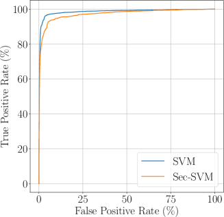
(a) ROC

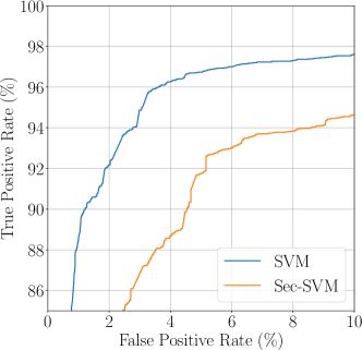
(b) ROC (Zoom)

Figure 2: Performance of SVM and Sec-SVM in absence of adversarial attacks.

Figure 2 reports the AUROC of SVM and Sec-SVM on the DREBIN feature space in absence of attacks. As expected [23], Sec-SVM sacrifices some detection performance in return for greater feature-space adversarial robustness.

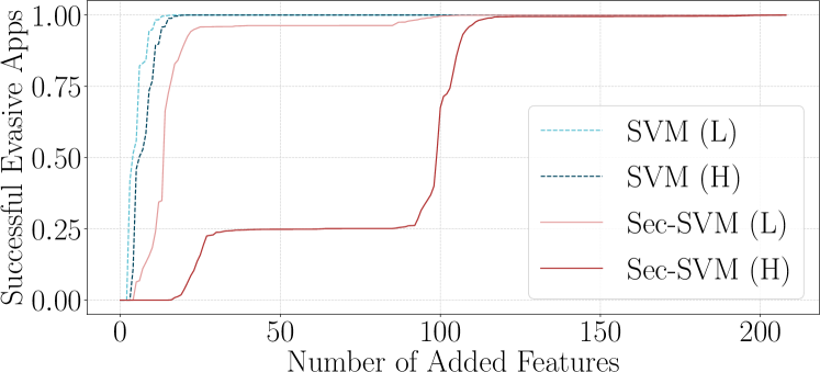
Figure 3: Cumulative distribution of features added to adversarial malware (out of a total 10,000 features remaining after feature selection).

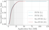
(a) Size

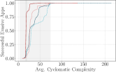
(b) Avg. CC

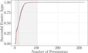
(c) Permissions

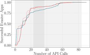
(d) API calls

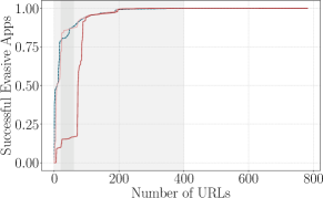
(e) URLs

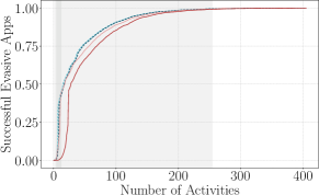
(f) Activities

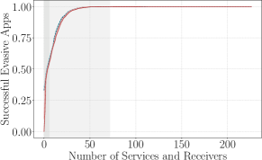
(g) Services and Receivers

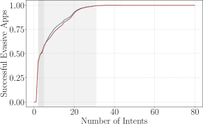
(h) Intents

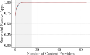
(i) Content Providers

Figure 4: Statistics of the evasive malware variants, compared with statistics of benign apps. The dark gray background highlights the area between first and third quartile of benign applications; the light gray background is based on the 3$\sigma$ rule and highlights values benign statistics between $0.15\%$ and $99.85\%$ of the distribution (i.e., spanning $99.7\%$ of the distribution).

Attack Success Rate. We perform our attack using true positive malware from the test set, i.e., all malware objects correctly classified as malware. We consider four settings depending on the defense algorithm and the attack confidence: SVM (L), SVM (H), Sec-SVM (L), and Sec-SVM (H). In absence of FlowDroid exceptions (see Appendix -G), we are able to create an evasive variant for each malware in all four configurations. In other words, we achieve a misclassification rate of 100.0% on the successfully generated apps, where the problem-space constraints are satisfied by construction (as defined in § III). Figure 3 reports the cumulative distribution of features added when generating evasive apps for the four different configurations. As expected, Sec-SVM requires the attacker to modify more features, but here we are no longer interested in the feature-space properties, since we are performing a problem-space attack. This demonstrates that measuring attacker effort with $l_{p}$ perturbations as in the original Sec-SVM evaluation [23] overestimates the robustness of the defense and is better assessed using our framework (§ II).

While the plausibility problem-space constraint is satisfied by design by transplanting only realistic existing code, it is informative to analyze how the statistics of the evasive malware relate to the corresponding distributions in benign apps. Figure 4 reports the cumulative distribution of app statistics across the four settings: the $X$-axis reports the statistics values, whereas the $Y$-axis reports the cumulative percentage of evasive malware apps. We also shade two gray areas: a dark gray area between the first quartile $q_{1}$ and third quartile $q_{3}$ of the statistics for the benign applications; the light gray area refers to the $3\sigma$ rule and reports the area within the 0.15% and 99.85% of the benign apps distribution.

Figure 4 shows that while evading Sec-SVM tends to cause a shift towards the higher percentiles of each statistic, the vast majority of apps falls within the gray regions in all configurations. We note that this is just a qualitative analysis to verify that the statistics of the evasive apps roughly align with those of benign apps; it is not sufficient to have an anomaly in one of these statistics to determine that an app is malicious (otherwise, very trivial rules could be used for malware detection itself, and this is not the case). We also observe that there is little difference between the statistics generated by Sec-SVM and by traditional SVM; this means that greater feature-space perturbations do not necessarily correspond to greater perturbations in the problem-space, reinforcing the feasibility and practicality of evading Sec-SVM.

Runtime Overhead. The time to perform the search strategy occurring in the feature space is almost negligible; the most demanding operation is in the actual code modification. Figure 5 depicts the distribution of injection times for our test set malware which is the most expensive operation in our approach while the rest is mostly pipeline overhead. The time spent per app is low: in most cases, less than 100 seconds, and always less than 2,000 seconds (~33 mins). The low runtime cost suggests that it is feasible to perform this attack at scale and reinforces the need for new defenses in this domain.

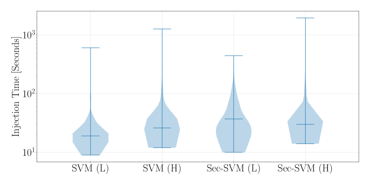
Figure 5: Violin plots of injection times per adversarial app.

V Discussion on Attack and Results

We provide some deeper discussion on the results of our novel problem-space attack.

Android Attack Effectiveness. We conclude that it is practically feasible to evade the state-of-the-art Android malware classifier DREBIN [8] and its hardened variant, Sec-SVM [23], and that we are able to automatically generate realistic and inconspicuous evasive adversarial applications, often in less than 2 minutes. This shows for the first time that it is possible to create realistic adversarial applications at scale.

Obfuscation. It could be argued that traditional obfuscation methods can be used to simply hide malicious functionality. The novel problem-space attack in this work evaluates the feasibility of an “adversarial-malware as a service” scenario, where the use of mass obfuscation may raise the suspicions of the defender; for example, antivirus companies often classify samples as malicious simply because they utilize obfuscation or packing [69, 67]. Moreover, some other analysis methods combine static and dynamic analysis to prioritize evaluation of code areas that are likely obfuscated [e.g., 42]. On the contrary, our transformations aim to be fully inconspicuous by adding only legitimate benign code and, to the best of our knowledge, we do not leave any relevant artifact in the process. While the effect on problem-space constraints may differ depending on the setting, attack methodologies such as ours and traditional obfuscation techniques naturally complement each other in aiding evasion and, in the program domain, code transplantation may be seen as a tool for developing new forms of inconspicuous obfuscation [27].

Defense Directions Against Our Attack. A recent promising direction by Incer et al. [34] studies the use of monotonic classifiers, where adding features can only increase the decision score (i.e., an attacker cannot rely on adding more features to evade detection); however, such classifiers require non-negligible time towards manual feature selection (i.e., on features that are harder for an attacker to change), and—at least in the context of Windows malware [34]—they suffer from high false positives and an average reduction in detection rate of 13%. Moreover, we remark that we decide to add goodware parts to malware for practical reasons: the opposite transplantation would be immediate to do if a dataset with annotated malicious bytecode segments were available. As part of future work we aim to investigate whether it would still be possible to evade monotonic classifiers by adding only a minimal number of malicious slices to a benign application.

Defenses Against Problem-Space Attacks. Unlike settings where feature and problem space are closely related (e.g., images and audio), limitations on feature-space $l_{p}$ perturbations are often insufficient to determine the risk and feasibility of an attack in the real world. Our novel problem-space formalization (§ II) paves the way to the study of practical defenses that can be effective in settings which lack an inverse feature mapping. Simulating and evaluating attacker capabilities in the problem space helps define realistic threat models with more constrained modifications in the feature space—which may lead to more robust classifier design. Our Android evasion attack (§ III) demonstrates for the first time that it is feasible to evade feature-space defenses such as Sec-SVM in the problem-space—and to do so en masse.

VI Related Work

Adversarial Machine Learning. Adversarial ML attacks have been studied for more than a decade [11]. These attacks aim to modify objects either at training time (poisoning [65]) or at test time (evasion [12]) to compromise the confidentiality, integrity, or availability of a machine learning model. Many formalizations have been proposed in the literature to describe feature-space attacks, either as optimization problems [12, 16] (see also § II-A for details) or game theoretic frameworks [21].

Problem-Space Attacks. Recently, research on adversarial ML has moved towards domains in which the feature mapping is not invertible or not differentiable. Here, the adversary needs to modify the objects in the problem space (i.e., input space) without knowing exactly how this will affect the feature space. This is known as the inverse feature-mapping problem [32, 12, 58]. Many works on problem-space attacks have been explored on different domains: text [43, 3], PDFs [46, 45, 41, 22, 74], Windows binaries [38, 59, 60], Android apps [23, 31, 75], NIDS [28, 6, 7, 20], ICS [76], and Javascript source code [58]. However, each of these studies has been conducted empirically and followed some inferred best practices: while they share many commonalities, it has been unclear how to compare them and what are the most relevant characteristics that should be taken into account while designing such attacks. Our formalization (§ II) aims to close this gap, and we show how it can be used to describe representative feature-space and problem-space attacks from the literature (§ II-C).

Adversarial Android Malware. This paper also proposes a novel adversarial problem-space attack in the Android domain (§ III); our attack overcomes limitations of existing proposals, which are evidenced through our formalization. The most related approaches to our novel attack are on attribution [58], and on adversarial malware generation [75, 60, 31]. Quiring et al. [58] do not consider malware detection, but design a set of simple mutations to change the programming style of an application to match the style of a target developer (e.g., replacing for loops with while loops). This strategy is effective for attribution, but is insufficient for malware detection as altering stylometric properties alone would not evade a malware classifier which captures program semantics. Moreover, it is not feasible to define a hardcoded set of transformations for all possible semantics—which may also leave artifacts in the mutated code. Conversely, our attack relies on automated software transplantation to ensure plausibility of the generated code and avoids hardcoded code mutation artifacts.

Grosse et al. [31] perform minimal modifications that preserve semantics, and only modify single lines of code in the Manifest; but these may be easily detected and removed due to unused permissions or undeclared classes. Moreover, they limit their perturbation to 20 features, whereas our problem-space constraints represent a more realistic threat model.

Yang et al. [75] propose a method for adversarial Android malware generation. Similarly to us, they rely on automated software transplantation [10] and evaluate their adversarial attack against the DREBIN classifier [8]. However, they do not formally define which semantics are preserved by their transformation, and their approach is extremely unstable, breaking the majority of apps they mutate (e.g., they report failures after 10+ modifications on average—which means they would likely not be able to evade Sec-SVM [23] which on average requires modifications of 50+ features). Moreover, the code is unavailable, and the paper lacks details required for reevaluating the approach, including any clear descriptions of preprocessing robustness. Conversely, our attack is resilient to the insertion of a large number of features (§ IV), preserves dynamic app semantics through opaque predicates (§ III-C), and is resilient against static program analysis (§ III-D).

Rosenberg et al. [60] propose a black-box adversarial attack against Windows malware classifiers that rely on API sequence call analysis—an evasion strategy that is also applicable to similar Android classifiers. In addition to the limited focus on API-based sequence features, their problem-space transformation leaves two major artifacts which could be detected through program analysis: the addition of no-operation instructions (no-ops), and patching of the import address table (IAT). Firstly, the inserted API calls need to be executed at runtime and so contain individual no-ops hardcoded by the authors following a practice of “security by obscurity”, which is known to be ineffective [37, 19]; intuitively, they could be detected and removed by identifying the tricks used by attackers to perform no-op API calls (e.g., reading 0 bytes), or by filtering the “dead” API calls (i.e., which did not perform any real task) from the dynamic execution sequence before feeding it to the classifier. Secondly, to avoid requiring access to the source code, the new API calls are inserted and called using IAT patching. However, all of the new APIs must be included in a separate segment of the binary and, as IAT patching is a known malicious strategy used by malware authors [25], IAT calls to non-standard dynamic linkers or multiple jumps from the IAT to an internal segment of the binary would immediately be identified as suspicious. Conversely, our attack does not require hardcoding and by design is resilient against traditional non-ML program analysis techniques.

VII Availability

We release the code and data of our approach to other researchers by responsibly sharing a private repository. The project website with instructions to request access is at: https://s2lab.kcl.ac.uk/projects/intriguing.

VIII Conclusions

Since the seminal work that evidenced intriguing properties of neural networks [66], the community has become more widely aware of the brittleness of machine learning in adversarial settings [11].

To better understand real-world implications across different application domains, we propose a novel formalization of problem-space attacks as we know them today, that enables comparison between different proposals and lays the foundation for more principled designs in subsequent work. We uncover new relationships between feature space and problem space, and provide necessary and sufficient conditions for the existence of problem-space attacks. Our novel problem-space attack shows that automated generation of adversarial malware at scale is a realistic threat—taking on average less than 2 minutes to mutate a given malware example into a variant that can evade a hardened state-of-the-art classifier.

-A Symbol Table

Table I provides a reference for notation and major symbols used throughout the paper.

TABLE I: Table of symbols.

Symbol	Description
$\mathcal{Z}$	Problem space (i.e., input space).
$\mathcal{X}$	Feature space $\mathcal{X}\subseteq\mathbb{R}^{n}$.
$\mathcal{Y}$	Label space.
$\varphi$	Feature mapping function $\varphi:\mathcal{Z}\longrightarrow\mathcal{X}$.
$h_{i}$	Discriminant function $h_{i}:\mathcal{X}\longrightarrow\mathbb{R}$ that assigns object $\bm{x}\in\mathcal{X}$ a score in $\mathbb{R}$ (e.g., distance from hyperplane) that represents fitness to class $i\in\mathcal{Y}$.
$g$	Classifier $g:\mathcal{X}\longrightarrow\mathcal{Y}$ that assigns object $\bm{x}\in\mathcal{X}$ to class $y\in\mathcal{Y}$. Also known as decision function. It is defined based on the output of the discriminant functions $h_{i},\forall i\in\mathcal{Y}$ .
$\mathcal{L}_{y}$	Loss function $\mathcal{L}_{y}:\mathcal{X}\times\mathcal{Y}\longrightarrow\mathbb{R}$ of object $\bm{x}\in\mathcal{X}$ with respect to class $y\in\mathcal{Y}$.
$f_{y,\kappa}$	Attack objective function $f_{y,\kappa}:\mathcal{X}\times\mathcal{Y}\times\mathbb{R}\longrightarrow\mathbb{R}$ of object $\bm{x}\in\mathcal{X}$ with respect to class $y\in\mathcal{Y}$ with maximum confidence $\kappa\in\mathbb{R}$.
$f_{y}$	Compact notation for $f_{y,0}$.
$\Omega$	Feature-space constraints.
$\bm{\delta}$	$\bm{\delta}\in\mathbb{R}^{n}$ is a symbol used to denote a feature-space perturbation vector.
$\bm{\eta}$	Side-effect feature vector.
$T$	Transformation $T:\mathcal{Z}\longrightarrow\mathcal{Z}$.
T	Transformation sequence $\text{\bf T}=T_{n}\circ T_{n-1}\circ\dots\circ T_{1}$.
$\mathcal{T}$	Space of available transformations.
$\Upsilon$	Suite of automated tests $\tau\in\Upsilon$ to verify preserved semantics.
$\Pi$	Suite of manual tests $\pi\in\Pi$ to verify plausibility. In particular, $\pi(z)=1$ if $z\in\mathcal{Z}$ is plausible, else $\pi(z)=0$.
$\Lambda$	Set of preprocessing operators $\text{\bf A}\in\Lambda$ for which $z\in\mathcal{Z}$ should be resistant (i.e., $\text{\bf A}(\text{\bf T}(z))=\text{\bf T}(z)$).
$\Gamma$	Problem-space constraints $\Gamma$, consisting of $\{\Pi,\Upsilon,\mathcal{T},\Lambda\}$.
$\mathcal{D}$	Training dataset.
$\bm{w}$	Model hyper-parameters.
$\Theta$	Knowledge space.
$\theta$	Threat model assumptions $\theta\in\Theta$; more specifically, $\theta=(\mathcal{D},\mathcal{X},g,\bm{w})$. A hat symbol is used if only estimates of parameters are known. See Section -B for details.

-B Threat Model

The threat model must be defined in terms of attacker knowledge and capability, as in related literature [11, 65, 19]. While the attacker knowledge is represented in the same way as in the traditional feature-space attacks, their capability also includes the problem-space constraints $\Gamma$. For completeness, we report the threat model formalization proposed in Biggio and Roli [11].

Attacker Knowledge. We represent the knowledge as a set $\theta\in\Theta$ which may contain (i) training data $\mathcal{D}$, (ii) the feature set $\mathcal{X}$, (iii) the learning algorithm $g$, along with the loss function $\mathcal{L}$ minimized during training, (iv) the model parameters/hyperparameters $\bm{w}$. A parameter is marked with a hat symbol if the attacker knowledge of it is limited or only an estimate (i.e., $\hat{\mathcal{D}}$, $\hat{\mathcal{X}}$, $\hat{g}$, $\hat{\bm{w}}$). There are three major scenarios [11]:

• Perfect Knowledge (PK) white-box attacks, in which the attacker knows all parameters and $\theta_{PK}=(\mathcal{D},\mathcal{X},g,\bm{w})$.

• Limited Knowledge (LK) gray-box attacks, in which the attacker has some knowledge on the target system. Two common settings are LK with Surrogate Data (LK-SD), where $\theta_{LK-SD}=(\hat{\mathcal{D}},\mathcal{X},g,\hat{\bm{w}})$, and LK with Surrogate Learners, where $\theta_{LK-SL}=(\hat{\mathcal{D}},\mathcal{X},\hat{g},\hat{\bm{w}})$. Knowledge of the feature space and the ability to collect surrogate data, $\theta\supseteq(\hat{\mathcal{D}},\mathcal{X})$, enables the attacker to perform mimicry attacks in which the attacker manipulates examples to resemble the high density region of the target class [12, 28].

• Zero Knowledge (ZK) black-box attacks, where the attacker has no information on the target system, but has some information on which kind of feature extraction is performed (e.g., only static analysis in programs, or structural features in PDFs). In this case, $\theta_{LK}=(\hat{\mathcal{D}},\hat{\mathcal{X}},\hat{g},\hat{\bm{w}})$.

Note that $\theta_{PK}$ and $\theta_{LK}$ imply knowledge of any defenses used to secure the target system against adversarial examples, depending on the degree to which each element is known [18].

Attacker Capability. The capability of an attacker is expressed in terms of his ability to modify feature space and problem space, i.e., the attacker capability is described through feature-space constraints $\Omega$ and problem-space constraints $\Gamma$.

We observe that the attacker’s knowledge and capability can also be expressed according to the FAIL [65] model as follows: knowledge of Features $\mathcal{X}$ (F), the learning Algorithm $g$ (A), Instances in training $\mathcal{D}$ (I), Leverage on feature space and problem space with $\Omega$ and $\Gamma$ (L).

More details on the threat models can be found in [11, 65].

-C Theorem Proofs

Proof of Theorem 1. We proceed with a proof by contradiction. Let us consider a problem-space object $z\in\mathcal{Z}$ with features $\bm{x}\in\mathcal{X}$, which we want to misclassify as a target class $t\in\mathcal{Y}$. Without loss of generality, we consider a low-confidence attack, with desired attack confidence $\kappa=0$ (see Equation 3). We assume by contradiction that there is no solution to the feature-space attack; more formally, that there is no solution $\bm{\delta}^{*}=\arg\min_{\bm{\delta}\in\mathbb{R}^{n}:\bm{\delta}\models\Omega}f_{t}(\bm{x}+\bm{\delta})$ that satisfies $f_{t}(\bm{x}+\bm{\delta}^{*})<0$. We now try to find a transformation sequence T such that $f_{t}(\varphi(\text{\bf T}(z)))<0$. Let us assume that $\text{\bf T}^{*}$ is a transformation sequence that corresponds to a successful problem-space attack. By definition, $\text{\bf T}^{*}$ is composed by individual transformations: a first transformation $T_{1}$, such that $\varphi(T_{1}(z))=\bm{x}+\bm{\delta}_{1}$; a second transformation $T_{2}$ such that $\varphi(T_{2}(T_{1}(z))=\bm{x}+\bm{\delta}_{1}+\bm{\delta}_{2}$; a $k$-th transformation $\varphi(T_{k}(\cdots T_{2}(T_{1}(z))))=\bm{x}+\sum_{k}\bm{\delta}_{k}$. We recall that the feature-space constraints are determined by the problem-space constraints, i.e., $\Gamma\vdash\Omega$, and that, with slight abuse of notation, we can write that $\Omega\subseteq\Gamma$; this means that the search space allowed by $\Gamma$ is smaller or equal than that allowed by $\Omega$. Let us now replace $\sum_{k}\bm{\delta}_{k}$ with $\bm{\delta}^{\dagger}$, which is a feature-space perturbation corresponding to the problem-space transformation sequence T, such that $f_{t}(\bm{x}+\bm{\delta}^{\dagger})<0$ (i.e., the sample is misclassified). However, since the constraints imposed by $\Gamma$ are stricter or equal than those imposed by $\Omega$, this means that $\bm{\delta}^{\dagger}$ must be a solution to $\arg\min_{\bm{\delta}\in\Omega}f_{t}(\bm{x}+\bm{\delta})$ such that $f_{t}(\bm{x}+\bm{\delta}^{\dagger})<0$. However, this is impossible, because we hypothesized that there was no solution for the feature-space attack under the constraints $\Omega$. Hence, having a solution in the feature-space attack is a necessary condition for finding a solution for the problem-space attack.

Proof of Theorem 2. The existence of a feature-space attack (Equation 11) is the necessary condition, which has been already proved for Theorem 1. Here, we need to prove that, with Equation 12, the condition is sufficient for the attacker to find a problem-space transformation that misclassifies the object. Another way to write Equation 12 is to consider that the attacker knows transformations that affect individual features only (modifying more than one feature will result as a composition of such transformations). Formally, for any object $z\in\mathcal{Z}$ with features $\varphi(z)=\bm{x}\in\mathcal{X}$, for any feature-space dimension $X_{i}$ of $\mathcal{X}$, and for any value $v\in domain(X_{i})$, let us assume the attacker knows a valid problem-space transformation sequence $\text{\bf T}:\text{\bf T}(z)\models\Gamma,\varphi(\text{\bf T}(z))=\bm{x}^{\prime}$, such that:

$$x_{i}^{\prime}=x_{i}+v,\qquad x_{i}\in\bm{x},x_{i}^{\prime}\in\bm{x}^{\prime}$$ (13)

$$x_{j}^{\prime}=x_{j},\qquad \forall j\neq i,x_{j}\in\bm{x},x_{j}^{\prime}\in\bm{x}^{\prime}$$ (14)

Intuitively, these two equations refer to the existence of a problem-space transformation T that affects only one feature $X_{i}$ in $\mathcal{X}$ by any amount $v\in domain(X_{i})$. In this way, given any adversarial feature-space perturbation $\bm{\delta}^{*}$, the attacker is sure to find a transformation sequence that modifies each individual feature step-by-step. In particular, let us consider $idx_{0},\dots,idx_{q-1}$ corresponding to the $q>0$ values in $\bm{\delta}^{*}$ that are different from 0 (i.e., values corresponding to an actual feature-space perturbation). Then, a transformation sequence $\text{\bf T}:\text{\bf T}(z)\models\Gamma,\text{\bf T}=\text{\bf T}^{idx_{q}-1}\circ\text{\bf T}^{idx_{q-2}}\circ\dots\circ\text{\bf T}^{idx_{0}}$ can always be constructed by the attacker to satisfy $\varphi(\text{\bf T}(z))=\bm{x}+\bm{\delta}^{*}$. We highlight that we do not consider the existence of a specific transformation in $\mathcal{Z}$ that maps to $\bm{x}+\bm{\delta}^{*}$ because that may not be known by the attacker; hence, the attacker may never learn such a specific transformation. Thus, Equation 12 must be valid for all possible perturbations within the considered feature space.

-D Opaque Predicates Generation

We use opaque predicates [4] as inconspicuous conditional statements always resolving to False to preserve dynamic semantics of the Android applications.

To ensure the intractability of such an analysis, we follow the work of Moser et al. [51] and build opaque predicates using a formulation of the 3-SAT problem such that resolving the truth value of the predicate is equivalent to solving the NP-complete 3-SAT problem.

The $k$-satisfiability ($k$-SAT) problem asks whether the variables of a Boolean logic formula can be consistently replaced with True or False in such a way that the entire formula evaluates to True; if so the formula is satisfiable. Such a formula is easily expressed in its conjunctive normal form:

$$\textstyle\bigwedge\nolimits_{i=1}^{m}(V_{i1}\vee V_{i2}\vee...\vee V_{ik})\,,$$

where $V_{ij}\in\{v_{1},v_{2},...,v_{n}\}$ are Boolean variables and $k$ is the number of variables per clause.

Importantly, when $k=3$, formulas are only NP-Hard in the worst case—30% of 3-SAT problems are in P [61]. This baseline guarantee is not sufficient as our injected code should never execute. Additionally, we require a large number of random predicates to reduce commonality between the synthetic portions of our generated examples.

To consistently generate NP-Hard k-SAT problems we use Random k-SAT [61] in which there are 3 parameters: the number of variables $n$, the number of clauses $m$, and the number of literals per clause $k$.

To construct a 3-SAT formula, $m$ clauses of length 3 are generated by randomly choosing a set of 3 variables from the $n$ available, and negating each with probability $50\%$. An empirical study by Selman et al. [61] showed that $n$ should be at least 40 to ensure the formulas are hard to resolve. Additionally, they show that formulas with too few clauses are under-constrained while formulas with too many clauses are over-constrained, both of which reduce the search time. These experiments led to the following conjecture.

Listing 1: Simplified example of an opaque predicate generated by JSketch. The opaque predicate wraps an adapted vein that calls a class containing benign features. Note that while we render the equivalent Java here for clarity, the actual transplantation occurs at a lower level of abstraction (Dalvik bytecode). The Random k-SAT parameters shown are our ideal parameters; in practice they are modulated around these values as part of the JSketch synthesis in order to avoid them becoming fingerprintable (e.g., having common length boolean arrays and loops between all predicates).

⬇

1 void opaque() {

2 Random random = new Random();

3 this();

4 boolean[] arrayOfBoolean = new boolean[40];

5 byte b1;

6 for (b1 = 0; b1 < arrayOfBoolean.length; b1++)

7 arrayOfBoolean[b1] = random.nextBoolean();

8 b1 = 1;

9 for (byte b2 = 0; b2 < 184.0D; b2++) {

10 boolean bool = false;

11 for (byte b = 0; b < 3; b++)

12 bool |= arrayOfBoolean[random.nextInt(arrayOfBoolean.length)];

13 if (!bool)

14 b1 = 0;

15 }

16 if (b1 != 0) {

17

18 // Beginning of adapted vein

19 Context context = ((Context)this).getApplicationContext();

20 Intent intent = new Intent();

21 this(this, h.a(this, cxim.qngg.TEhr.sFiQa.class));

22 intent.putExtra(”l”, h.p(this));

23 intent.addFlags(268435456);

24 startActivity(intent);

25 h.x(this);

26 return;

27 // End of adapted vein

28

29 }

30 }

Threshold Conjecture [61]. Let us define $c^{*}$ as the threshold at which 50% of the formulas are satisfiable. For $m/n<c^{*}$, as $n\rightarrow\infty$, the formula is satisfiable with probability $100\%$, and for $m/n>c^{*}$, as $n\rightarrow\infty$, the formula is unsatisfiable with probability $100\%$.

The current state-of-the-art for $c^{*}$ is $3.42<c^{*}\approx 4.3<4.51$ for 3-SAT [61, 36, 50]. We use this conjecture to ensure that the formulas used for predicates are unsatisfiable with high probability, i.e., that the predicate is likely a contradiction and will always evalute to False.

Additionally we discard any generated formulas that fall into two special cases of 3-SAT that are polynomially solvable:

• 2-SAT: The construction may be 2-SAT if it can be expressed as a logically equivalent 2CNF formula [40].

• Horn-SAT: If at most one literal in a clause is positive, it is a Horn clause. If all clauses are Horn clauses, the formula is Horn-SAT and solvable in linear time [24].

We tested 100M Random 3-SAT trials using the fixed clause-length model with parameters $n\simeq 40,m\simeq 184,c^{*}\simeq 4.6$. All (100%) of the generated constructions were unsatisfiable (and evaluated to False at runtime) which aligns with the findings of Selman et al. [61]. This probability is sufficient to prevent execution with near certainty.

To further reduce artifacts introduced by reusing the same predicate, we use JSketch [35], a sketch-based program synthesis tool, to randomly generate new predicates prior to injection with some variation while maintaining the required properties. Post-transplantation, we verify for each adversarial example that Soot’s program optimizations have not been able to recognize and eliminate them. An example of a generated opaque predicate (rendered in equivalent Java rather than Dalvik bytecode) is shown in LABEL:lst:opaque.

-E DREBIN and Sec-SVM Implementation Details

We have access to a working Python implementation of DREBIN based on sklearn, androguard, and aapt, and we rely on LinearSVC classifier with C=1.

We now describe the details of our implementation of the Sec-SVM approach [23]. To have have full control of the training procedure, we approximate the linear SVM as a single-layer neural network (NN) using PyTorch [53]. We recall that the main intuition behind Sec-SVM is that classifier weights are distributed more evenly in order to force an attacker to modify more features to evade detection. Hence, we modify the training procedure so that the Sec-SVM weights are bounded by a maximum weight value $k$ at each training optimization step. Similarly to Demontis et al. [23], we perform feature selection for computational efficiency, since PyTorch does not support sparse vectors. We use an $l_{2}$ (Ridge) regularizer to select the top 10,000 with negligible reduction in AUROC. This performance retention follows from recent results that shows SVM tends to overemphasize a subset of features [48]. To train the Sec-SVM, we perform an extensive hyperparameter grid-search: with Adam and Stochastic Gradient Descent (SGD) optimizers; training epochs of 5 to 100; batch sizes from $2^{0}$ to $2^{12}$; learning rate from $10^{0}$ to $10^{-5}$. We identify the best single-layer NN configuration for our training data to have the following parameters: Stochastic Gradient Descent (SGD), batch size 1024, learning rate $10^{-4}$, and 75 training epochs. We then perform a grid-search of the Sec-SVM hyperparameter $k$ (i.e., the maximum weight absolute value [23]) by clipping weights during training iterations. We start from $k=w_{max}$, where $w_{max}=\max_{i}(w_{i})$ for all features $i$; we then continue reducing $k$ until we reach a weight distribution similar to that reported in [23], while allowing a maximum performance loss of $2\%$ in AUROC. In this way, we identify the best value for our setting as $k=0.2$.

In § IV, Figure 2 reported the AUROC for the DREBIN classifier [8] in SVM and Sec-SVM modes. The SVM mode has been evaluated using the LinearSVC class of scikit-learn [54] that utilizes the LIBLINEAR library [26]; as in the DREBIN paper [8], we use hyperparameter C=1. The performance degradation of the Sec-SVM compared to the baseline SVM shown in Figure 2 is in part related to the defense itself (as detailed in [23]), and in part due to minor convergence issues (since our single-layer NN converges less effectively than the LIBLINEAR implementation of scikit-learn). We have verified with Demontis et al. [23] the correctness of our Sec-SVM implementation and its performance, for the analysis performed in this work.

-F Attack Algorithms

Algorithm 1 and Algorithm 2 describe in detail the two main phases of our search strategy: organ harvesting and adversarial program generation. For the sake of simplicity, we describe a low-confidence attack, i.e., the attack is considered successful as soon as the classification score is below zero. It is immediate to consider high-confidence variations (as we evaluate in § IV).

Note that when using the minimal injection host $z_{min}$ to calculate the features that will be induced by a gadget, features in the corresponding feature vector $\bm{x}_{min}$ should be noted and dealt with accordingly (i.e., discounted). In our case $x_{min}$ contained the following three features:

{ "intents::android_intent_action_MAIN":1,  "intents::android_intent_category_LAUNCHER":1,  "activities::_MainActivity":1}

Input: Discriminant function $h(\bm{x})=\bm{w}^{T}\bm{x}+b$, which classifies $\bm{x}$ as malware if $h(\bm{x})>0$, otherwise as goodware. Minimal app $z_{min}\in\mathcal{Z}$ with features $\varphi(z_{min})=\bm{x}_{min}$.

Parameters : Number of features to consider $n_{f}$; number of donors per-feature $n_{d}$.

Output: Ice-box of harvested organs with feature vectors.

1  ice-box $\leftarrow$ {} $\triangleright$ Empty key-value dictionary.

2 $L\leftarrow$ List of pairs ($w_{i}$, $i$), sorted by increasing value of $w_{i}$.

3 $L^{\prime}\leftarrow$ First $n_{f}$ elements of $L$, then remove any entry with $w_{i}\geq 0$.

4 for $(w_{i},i)$ in $L^{\prime}$ do

5       ice-box[i] $\leftarrow$ [] $\triangleright$ Empty list for gadgets with feature $i$.

6       while length(ice-box[i])$<n_{d}$ do

7             $z_{j}\leftarrow$ Randomly sample a benign app with feature $x_{i}=1$.

8             Extract gadget $\rho_{j}\in\mathcal{Z}$ with feature $x_{i}=1$ from $z_{j}$.

9             $s\leftarrow$ Software stats of $\rho_{j}$

10             $z^{\prime}\leftarrow$ Inject gadget $\rho_{j}$ in app $z_{min}$.

11             $(\bm{x}_{min}\vee\bm{e}_{i}\vee\bm{\eta}_{j})\leftarrow\varphi(z^{\prime})$ $\triangleright$ $\bm{e}_{i}$ is a one-hot vector.

12             $\bm{r}_{j}\leftarrow(\bm{e}_{i}\vee\bm{\eta}_{j})\leftarrow\varphi(z^{\prime})\wedge\neg\bm{x}_{min}$ $\triangleright$ Gadget features obtained through set difference.

13             if $h(\bm{r}_{j})>0$ then

14                   Discard the gadget;

15            else

16                   Append $(\rho_{j},\bm{r}_{j},s)$ to ice-box[i]. $\triangleright$ Store gadget

return ice-box;

Algorithm 1 Initialization (Ice-Box Creation)

Input: Discriminant function $h(\bm{x})=\bm{w}^{T}\bm{x}+b$, which classifies $\bm{x}$ as malware if $h(\bm{x})>0$, otherwise as goodware. Malware app $z\in\mathcal{Z}$. Ice-box $G$.

Parameters : Problem-space constraints.

Output: Adversarial app $z^{\prime}\in\mathcal{Z}$ such that $h(\varphi(z^{\prime}))<0$.

1  $\mathcal{T}\leftarrow$ Transplantation through gadget addition.

2 $\Upsilon\leftarrow$ Smoke test through app installation and execution in emulator.

3 $\Pi\leftarrow$ Plausibility by-design through code consolidation.

4 $\Lambda\leftarrow$ Artifacts from last column of LABEL:tab:instantiations.

5 $\Gamma\leftarrow\{\mathcal{T},\Upsilon,\Pi,\Lambda\}$

6 $s_{z}\leftarrow$ Software stats of $z$

7 $\bm{x}\leftarrow\varphi(z)$

8 $L\leftarrow$ [] $\triangleright$ Empty list.

9 $\text{\bf T}(z)\leftarrow$ Empty sequence of problem-space transformations.

10 for $(\rho_{j},\bm{r}_{j},s)$ in $G$ do

11       $\bm{d}_{j}\leftarrow\bm{r}_{j}\wedge\neg\bm{x}$ $\triangleright$ Feature-space contribution of gadget $j$.

12       $score_{j}\leftarrow h(\bm{d}_{j})$ $\triangleright$ Impact on decision score.

13       Append the pair $(score_{j},i,j)$ to $L$ $\triangleright$ Feature $i$, Gadget $j$.

14$L^{\prime}\leftarrow$ Sort $L$ by increasing $score_{j}$ $\triangleright$ Negative scores first.

15 for $(score_{j},i,j)$ in $L^{\prime}$ do

16       if z has $x_{i}=1$ then

17             Do nothing; $\triangleright$ Feature $i$ already present.

18      else if z has $x_{i}=0$ then

19             $(\rho_{j},\bm{r}_{j},s)\leftarrow$ element $j$ in ice-box $G$

20             if check_feasibility($s_{z}$, $s$) is True then

21                   $\bm{x}\leftarrow(\bm{x}\vee\bm{e}_{i}\vee\bm{\eta}_{j})$ $\triangleright$ Update features of $z$.

22                   Append transplantation $T\in\mathcal{T}$ of gadget $\rho_{j}$ in $\text{\bf T}(z)$.

23                   if $h(\bm{x})<0$ then

24                         Exit from cycle; $\triangleright$ Attack gadgets found.

25$z^{\prime}\leftarrow$ Apply transformation sequence $\text{\bf T}(z)$ $\triangleright$ Inject chosen gadgets.

26 if $h(\varphi(z^{\prime}))<0$ and $\text{\bf T}(z)\models\Gamma$ then

27       return z’; $\triangleright$ Attack successful.

28else

29       return Failure;

Algorithm 2 Attack (Adv. Program Generation)

-G FlowDroid Errors

We performed extensive troubleshooting of FlowDroid [9] to reduce the number of transplantation failures, and the transplantations without FlowDroid errors in the different configurations are as follows: 89.5% for SVM (L), 85% for SVM (H), 80.4% for Sec-SVM (L), 73.3% for Sec-SVM (H). These failures are only related to bugs and corner cases of the research prototype of FlowDroid, and do not pose any theoretical limitation on the attacks. Some examples of the errors encountered include: inability to output large APKs when the app’s SDK version is less than 21; a bug triggered in AXmlWriter, the third party component used by FlowDroid, when modifying app Manifests; and FlowDroid injecting system libraries found on the classpath when they should be excluded.

References

- Aho et al. [2007] A. V. Aho, R. Sethi, and J. D. Ullman. Compilers, Principles,Techniques, and Tools (2nd Edition). Addison Wesley, 2007.
- Allix et al. [2016] K. Allix, T. F. Bissyandé, J. Klein, and Y. Le Traon. Androzoo: Collecting Millions of Android Apps for the Research Community. In ACM Mining Software Repositories (MSR), 2016.
- Alzantot et al. [2018] M. Alzantot, Y. Sharma, A. Elgohary, B.-J. Ho, M. Srivastava, and K.-W. Chang. Generating natural language adversarial examples. In Empirical Methods in Natural Language Processing (EMNLP, 2018.
- Andreas Moser [2007] E. K. Andreas Moser, Christopher Kruegel. Limits of static analysis for malware detection. 2007.
- Android [2020] Android. Permissions overview - dangerous permissions, 2020. URL https://developer.android.com/guide/topics/permissions/overview#dangerous_permissions.
- Apruzzese and Colajanni [2018] G. Apruzzese and M. Colajanni. Evading Botnet Detectors Based on Flows and Random Forest with Adversarial Samples. In IEEE NCA, 2018.
- Apruzzese et al. [2019] G. Apruzzese, M. Colajanni, and M. Marchetti. Evaluating the effectiveness of Adversarial Attacks against Botnet Detectors. In IEEE NCA, 2019.
- Arp et al. [2014] D. Arp, M. Spreitzenbarth, M. Hubner, H. Gascon, and K. Rieck. DREBIN: Effective and Explainable Detection of Android Malware in Your Pocket. In NDSS, 2014.
- Arzt et al. [2014] S. Arzt, S. Rasthofer, C. Fritz, E. Bodden, A. Bartel, J. Klein, Y. L. Traon, D. Octeau, and P. D. McDaniel. Flowdroid: precise context, flow, field, object-sensitive and lifecycle-aware taint analysis for android apps. In PLDI. ACM, 2014.
- Barr et al. [2015] E. T. Barr, M. Harman, Y. Jia, A. Marginean, and J. Petke. Automated software transplantation. In ISSTA. ACM, 2015.
- Biggio and Roli [2018] B. Biggio and F. Roli. Wild patterns: Ten years after the rise of adversarial machine learning. Pattern Recognition, 2018.
- Biggio et al. [2013a] B. Biggio, I. Corona, D. Maiorca, B. Nelson, N. Šrndić, P. Laskov, G. Giacinto, and F. Roli. Evasion attacks against machine learning at test time. In ECML-PKDD. Springer, 2013a.
- Biggio et al. [2013b] B. Biggio, G. Fumera, and F. Roli. Security evaluation of pattern classifiers under attack. IEEE TKDE, 2013b.
- Bishop [2006] C. M. Bishop. Pattern Recognition and Machine Learning. 2006.
- Carlini [2019] N. Carlini. List of Adversarial ML Papers, 2019. URL https://nicholas.carlini.com/writing/2019/all-adversarial-example-papers.html.
- Carlini and Wagner [2017a] N. Carlini and D. Wagner. Towards evaluating the robustness of neural networks. In IEEE Symp. S&P, 2017a.
- Carlini and Wagner [2018] N. Carlini and D. Wagner. Audio adversarial examples: Targeted attacks on speech-to-text. In Deep Learning for Security (DLS) Workshop. IEEE, 2018.
- Carlini and Wagner [2017b] N. Carlini and D. A. Wagner. Adversarial examples are not easily detected: Bypassing ten detection methods. In AISec@CCS, pages 3–14. ACM, 2017b.
- Carlini et al. [2019] N. Carlini, A. Athalye, N. Papernot, W. Brendel, J. Rauber, D. Tsipras, I. Goodfellow, and A. Madry. On evaluating adversarial robustness. arXiv preprint arXiv:1902.06705, 2019.
- Corona et al. [2013] I. Corona, G. Giacinto, and F. Roli. Adversarial attacks against intrusion detection systems: Taxonomy, solutions and open issues. Information Sciences, 2013.
- Dalvi et al. [2004] N. Dalvi, P. Domingos, S. Sanghai, D. Verma, et al. Adversarial classification. In KDD. ACM, 2004.
- Dang et al. [2017] H. Dang, Y. Huang, and E. Chang. Evading classifiers by morphing in the dark. In ACM Conference on Computer and Communications Security, pages 119–133. ACM, 2017.
- Demontis et al. [2017] A. Demontis, M. Melis, B. Biggio, D. Maiorca, D. Arp, K. Rieck, I. Corona, G. Giacinto, and F. Roli. Yes, machine learning can be more secure! a case study on android malware detection. IEEE Transactions on Dependable and Secure Computing, 2017.
- Dowling and Gallier [1984] W. F. Dowling and J. H. Gallier. Linear-time algorithms for testing the satisfiability of propositional horn formulae. J. Log. Program., 1(3):267–284, 1984.
- Eresheim et al. [2017] S. Eresheim, R. Luh, and S. Schrittwieser. The evolution of process hiding techniques in malware-current threats and possible countermeasures. Journal of Information Processing, 2017.
- Fan et al. [2008] R. Fan, K. Chang, C. Hsieh, X. Wang, and C. Lin. LIBLINEAR: A library for large linear classification. J. Mach. Learn. Res., 9:1871–1874, 2008.
- Fass et al. [2019] A. Fass, M. Backes, and B. Stock. HideNoSeek: Camouflaging Malicious JavaScript in Benign ASTs. In ACM CCS, 2019.
- Fogla and Lee [2006] P. Fogla and W. Lee. Evading network anomaly detection systems: formal reasoning and practical techniques. In ACM Conference on Computer and Communications Security, pages 59–68. ACM, 2006.
- Goodfellow et al. [2016] I. Goodfellow, Y. Bengio, and A. Courville. Deep Learning. MIT press, 2016.
- Goodfellow et al. [2015] I. J. Goodfellow, J. Shlens, and C. Szegedy. Explaining and harnessing adversarial examples. In ICLR (Poster), 2015.
- Grosse et al. [2017] K. Grosse, N. Papernot, P. Manoharan, M. Backes, and P. McDaniel. Adversarial examples for malware detection. In ESORICS. Springer, 2017.
- Huang et al. [2011a] L. Huang, A. D. Joseph, B. Nelson, B. I. Rubinstein, and J. Tygar. Adversarial machine learning. In AISec. ACM, 2011a.
- Huang et al. [2011b] L. Huang, A. D. Joseph, B. Nelson, B. I. Rubinstein, and J. Tygar. Adversarial machine learning. In Proceedings of the 4th ACM workshop on Security and artificial intelligence, pages 43–58. ACM, 2011b.
- Incer et al. [2018] I. Incer, M. Theodorides, S. Afroz, and D. Wagner. Adversarially robust malware detection using monotonic classification. In Proc. Int. Workshop on Security and Privacy Analytics. ACM, 2018.
- Jeon et al. [2015] J. Jeon, X. Qiu, J. S. Foster, and A. Solar-Lezama. Jsketch: sketching for java. In ESEC/SIGSOFT FSE, pages 934–937. ACM, 2015.
- Kamath et al. [1994] A. Kamath, R. Motwani, K. V. Palem, and P. G. Spirakis. Tail bounds for occupancy and the satisfiability threshold conjecture. In FOCS, pages 592–603. IEEE Computer Society, 1994.
- Kerckhoffs [1883] A. Kerckhoffs. La cryptographie militaire. In Journal des sciences militaires, 1883.
- Kolosnjaji et al. [2018] B. Kolosnjaji, A. Demontis, B. Biggio, D. Maiorca, G. Giacinto, C. Eckert, and F. Roli. Adversarial malware binaries: Evading deep learning for malware detection in executables. In EUSIPCO. IEEE, 2018.
- Kulynych et al. [2018] B. Kulynych, J. Hayes, N. Samarin, and C. Troncoso. Evading classifiers in discrete domains with provable optimality guarantees. CoRR, abs/1810.10939, 2018.
- Larrabee [1992] T. Larrabee. Test pattern generation using boolean satisfiability. IEEE Trans. on CAD of Integrated Circuits and Systems, 11(1):4–15, 1992.
- Laskov and Šrndić [2011] P. Laskov and N. Šrndić. Static Detection of Malicious JavaScript-Bearing PDF Documents. In ACSAC. ACM, 2011.
- Leslous et al. [2017] M. Leslous, V. V. T. Tong, J.-F. Lalande, and T. Genet. Gpfinder: tracking the invisible in android malware. In MALWARE. IEEE, 2017.
- Li et al. [2019] J. Li, S. Ji, T. Du, B. Li, and T. Wang. Textbugger: Generating adversarial text against real-world applications. In NDSS. The Internet Society, 2019.
- Lowd and Meek [2005] D. Lowd and C. Meek. Good word attacks on statistical spam filters. In CEAS, volume 2005, 2005.
- Maiorca et al. [2012] D. Maiorca, G. Giacinto, and I. Corona. A Pattern Recognition System for Malicious PDF Files Detection. In Intl. Workshop on Machine Learning and Data Mining in Pattern Recognition. Springer, 2012.
- Maiorca et al. [2013] D. Maiorca, I. Corona, and G. Giacinto. Looking at the bag is not enough to find the bomb: an evasion of structural methods for malicious pdf files detection. In ASIACCS. ACM, 2013.
- Maiorca et al. [2019] D. Maiorca, B. Biggio, and G. Giacinto. Towards robust detection of adversarial infection vectors: Lessons learned in pdf malware. arXiv preprint, 2019.
- Melis et al. [2018] M. Melis, D. Maiorca, B. Biggio, G. Giacinto, and F. Roli. Explaining black-box android malware detection. In EUSIPCO. IEEE, 2018.
- Miller et al. [2016] B. Miller, A. Kantchelian, M. C. Tschantz, S. Afroz, R. Bachwani, R. Faizullabhoy, L. Huang, V. Shankar, T. Wu, G. Yiu, et al. Reviewer Integration and Performance Measurement for Malware Detection. In DIMVA. Springer, 2016.
- Mitchell et al. [1992] D. Mitchell, B. Selman, and H. Levesque. Hard and easy distributions of sat problems. In Proceedings of the Tenth National Conference on Artificial Intelligence, AAAI’92, pages 459–465. AAAI Press, 1992. ISBN 0-262-51063-4. URL http://dl.acm.org/citation.cfm?id=1867135.1867206.
- Moser et al. [2007] A. Moser, C. Kruegel, and E. Kirda. Limits of static analysis for malware detection. In ACSAC, 2007.
- Papernot et al. [2016] N. Papernot, P. McDaniel, S. Jha, M. Fredrikson, Z. B. Celik, and A. Swami. The limitations of deep learning in adversarial settings. In 2016 IEEE European Symposium on Security and Privacy (EuroS&P), pages 372–387. IEEE, 2016.
- Paszke et al. [2017] A. Paszke, S. Gross, S. Chintala, G. Chanan, E. Yang, Z. DeVito, Z. Lin, A. Desmaison, L. Antiga, and A. Lerer. Automatic differentiation in PyTorch. In NIPS Autodiff Workshop, 2017.
- Pedregosa et al. [2011] F. Pedregosa, G. Varoquaux, A. Gramfort, V. Michel, B. Thirion, O. Grisel, M. Blondel, P. Prettenhofer, R. Weiss, V. Dubourg, J. Vanderplas, A. Passos, D. Cournapeau, M. Brucher, M. Perrot, and E. Duchesnay. Scikit-Learn: Machine Learning in Python. Journal of Machine Learning Research, 12:2825–2830, 2011.
- Pendlebury et al. [2019] F. Pendlebury, F. Pierazzi, R. Jordaney, J. Kinder, and L. Cavallaro. TESSERACT: Eliminating Experimental Bias in Malware Classification across Space and Time. In 28th USENIX Security Symposium, Santa Clara, CA, 2019. USENIX Association. USENIX Sec.
- Pennington et al. [2014] J. Pennington, R. Socher, and C. D. Manning. Glove: Global vectors for word representation. In EMNLP, pages 1532–1543. ACL, 2014.
- Pierce and Benjamin [2002] B. C. Pierce and C. Benjamin. Types and programming languages. MIT press, 2002.
- Quiring et al. [2019] E. Quiring, A. Maier, and K. Rieck. Misleading authorship attribution of source code using adversarial learning. USENIX Security Symposium, 2019.
- Raff et al. [2018] E. Raff, J. Barker, J. Sylvester, R. Brandon, B. Catanzaro, and C. K. Nicholas. Malware detection by eating a whole exe. In AAAI Workshops, 2018.
- Rosenberg et al. [2018] I. Rosenberg, A. Shabtai, L. Rokach, and Y. Elovici. Generic black-box end-to-end attack against state of the art API call based malware classifiers. In RAID. Springer, 2018.
- Selman et al. [1996] B. Selman, D. G. Mitchell, and H. J. Levesque. Generating hard satisfiability problems. Artif. Intell., 81(1-2):17–29, 1996. doi: 10.1016/0004-3702(95)00045-3. URL https://doi.org/10.1016/0004-3702(95)00045-3.
- Sharif et al. [2016] M. Sharif, S. Bhagavatula, L. Bauer, and M. K. Reiter. Accessorize to a crime: Real and stealthy attacks on state-of-the-art face recognition. In ACM CCS. ACM, 2016.
- Smutz and Stavrou [2012] C. Smutz and A. Stavrou. Malicious pdf detection using metadata and structural features. In ACSAC. ACM, 2012.
- Šrndic and Laskov [2013] N. Šrndic and P. Laskov. Detection of malicious pdf files based on hierarchical document structure. In NDSS, 2013.
- Suciu et al. [2018] O. Suciu, R. Mărginean, Y. Kaya, H. Daumé III, and T. Dumitraş. When Does Machine Learning FAIL? Generalized Transferability for Evasion and Poisoning Attacks. USENIX Security Symposium, 2018.
- Szegedy et al. [2014] C. Szegedy, W. Zaremba, I. Sutskever, J. Bruna, D. Erhan, I. Goodfellow, and R. Fergus. Intriguing properties of neural networks. ICLR, 2014.
- Ugarte-Pedrero et al. [2015] X. Ugarte-Pedrero, D. Balzarotti, I. Santos, and P. G. Bringas. Sok: Deep packer inspection: A longitudinal study of the complexity of run-time packers. In IEEE Symposium on Security and Privacy, 2015.
- Vallée-Rai et al. [2010] R. Vallée-Rai, P. Co, E. Gagnon, L. Hendren, P. Lam, and V. Sundaresan. Soot: A java bytecode optimization framework. In CASCON First Decade High Impact Papers. IBM Corp., 2010.
- Vigna and Balzarotti [2018] G. Vigna and D. Balzarotti. When malware is packin’ heat. In USENIX ENIGMA, 2018.
- VirusTotal [2004] VirusTotal. VirusTotal, 2004. URL https://www.virustotal.com.
- Weiser [1981] M. Weiser. Program slicing. In Proceedings of the 5th International Conference on Software Engineering, ICSE ’81, pages 439–449. IEEE Press, 1981. URL http://dl.acm.org/citation.cfm?id=800078.802557.
- Weiss and D’Mello [2015] W. Weiss and C. D’Mello. Fundamentals of Model Theory. University of Toronto, 2015.
- Xiao et al. [2019] Q. Xiao, Y. Chen, C. Shen, Y. Chen, and K. Li. Seeing is not believing: Camouflage attacks on image scaling algorithms. In USENIX Security Symposium, pages 443–460. USENIX Association, 2019.
- Xu et al. [2016] W. Xu, Y. Qi, and D. Evans. Automatically evading classifiers. In NDSS, 2016.
- Yang et al. [2017] W. Yang, D. Kong, T. Xie, and C. A. Gunter. Malware detection in adversarial settings: Exploiting feature evolutions and confusions in android apps. In ACSAC. ACM, 2017.
- Zizzo et al. [2019] G. Zizzo, C. Hankin, S. Maffeis, and K. Jones. Adversarial machine learning beyond the image domain. In ACM DAC, 2019.