Spin-orbit Interaction driven Topological Features in a Quantum Ring

Abstract

One-dimensional quantum rings with Rashba and Dresselhaus spin-orbit couplings are studied analytically and are in perfect agreement with the numerical results. The topological charge of the spin field defined by the winding number along the ring is also studied analytically and numerically in the presence of the spin-orbit interactions. We also demonstrate the cases where the one-dimensional model is invalid for a relatively large radius. However, the numerical results of the two-dimensional model always remain reliable. Just as many physical properties of the quantum rings are influenced by the Aharonov-Bohm effect, the topological charge is also found to vary periodically due to the step-like change of the angular momentum with an increase of the magnetic field. This is significantly different from the cases of quantum dots. We also study how the current is induced by the magnetic field and spin-orbit couplings, which is strong enough that it could to be detected. The magnetic induction lines induced by the spin field and the current are also analyzed which can be observed and could perhaps help identifying the topological features of the spin fields in a quantum ring.

I Introduction

In the study of topological properties of condensed matter states, the crucially important role of the spin-orbit coupling (SOC) has been recognized in recent years TP03 ; TP04 ; tokura ; sky01 ; sky02 . It is important in the transport properties of the quantum Hall systems ezawa , such as silicene/germanene si and bilayer graphene abergel ; wang_2010 ; bilayerg (where there is pseudospin-orbit coupling). The nontrivial topological bands in the momentum space explicitly lead to ballistic transport at the edge of the topological insulator. Here we report on the topology of the spin texture in real space and its influence on the persistent current when the spin fields are topologically nontrivial in a quantum ring. Additionally, the persistent current and the spin fields induce effective magnetic fields which are found to be strong enough and can be observed.

Spin textures in real space in both noninteracting and interacting quantum dots maksym ; QD_book ; QD01 ; QD03 ; QD04 ; QD05 ; qd6 with the SOCs have been studied recently luo1 ; luo2 . The winding number was previously introduced to describe the topological charge $q$ of the spin field, and the topology of the in-plane spin texture can be tuned by the external electric and magnetic fields luo1 ; luo2 . The detection of the topological charge in low-dimensional systems is difficult but can be found in an indirect way, i.e., by measuring the sign of the $z$ component of the spin $\langle\sigma_{z}\rangle$ in a large dot. Since the sign of $\langle\sigma_{z}\rangle$ can be inverse in weak magnetic fields in the presence of the SOC the topological charge induced by the SOC can then be determined luo1 . Experimental determination of the topological winding number by polarized resonant X-ray scattering process winding_nature could also be a possibility.

The quantum ring ring1 ; Lucignano ; chapter ; maxwelldemon , which is yet another two-dimensional (2D) nano-device, has a similar Hamiltonian as that of the quantum dot. However, the quantum ring has its own features that are essentially different from the dot, since the geometric structure of the ring with different confining potential in the Hamiltonian introduces the magnetic flux into the system. Interestingly, we found that the one-dimensional (1D) model is not appropriate in the analysis of spin textures in a ring of large radius. It fails to explain the spin rotation in the radial direction which can however be found numerically in the 2D model. It is because the radial degree of freedom is integrated out in the 1D model, but this degree of freedom is important, especially when the radius of the ring is large. This size effect is associated with the flip of $\langle\sigma_{z}\rangle$, that can be observed experimentally.

Spin textures with topological charges are expected to appear in a ring due to the broken translational symmetry. Note that due to the geometry differences, the spin textures in quantum rings are very different from those in quantum dots. It can also be seen from the change of the $z$ component of the angular momentum, $\langle L_{z}\rangle$. In the single-electron case, $\langle L_{z}\rangle$ in a quantum dot varies from $0$ to $-1$ with the increase of the magnetic field $B$. Then the topological charge may be changed from $q=\mathrm{sgn}(g)$ to $q=-\mathrm{sgn}(g)$ where $g$ is the Landé factor of the material when both of the SOCs are present luo2 . In contrast, $\langle L_{z}\rangle$ changes gradually to $-\infty$ in a ring. Hence, we believe that the topological charge in a quantum ring will be changed more than once since the wave function highly depends on the $\langle L_{z}\rangle$. In our analysis that follows, we shall see that $q$ is indeed changed periodically with the increase of the magnetic field, as the ground state is changed when the magnetic flux increases by a magnetic flux quanta.

Considering the geometric structure of the ring, we then explore the current induced by both the magnetic field and the SOCs. In fact, the SOCs can be treated as an effective magnetic field, which then induces a local current even at zero magnetic field. Our results are comparable to the previous results where only one-dimensional ring was considered sheng . The two SOCs compete with each other to determine the vorticity of the current field. We note that the current flows locally but there is no net current, since the electron is confined locally in the ring. The magnetic fields induced by the current and the spin of the electron are also calculated in a semi-classical treatment. Both the current and the induced magnetic fields may actually be detected, and the measurements will be related to the topological features of the spin fields.

The paper is organized as follows. In Section II, we introduce the Hamiltonian of the quantum ring with Rashba and Dresselhaus SOCs, and define the spin field and its winding number. The current field is also defined there. In Section III, we simplify the Hamiltonian in the 1D limit. In a finite magnetic field, the Hamiltonian with Zeeman coupling is analyzed perturbatively. In Section IV, we study the spin textures of the electron in a quantum ring. In fact, we analyze the spin textures in the one-dimensional model and the results can be verified numerically in a two-dimensional ring. We then evaluate the current in the first-order perturbation theory and also numerically. It includes two parts: one that is induced by the magnetic field while the other is induced by the SOCs. The magnetic fields caused by the current and spin field are also calculated in Sec. III.C. In Sec. IV, we explain the limitations of the 1D model. We show that the spin rotates with the increase of the radius only when the ring is two-dimensional. Finally, we close with summary and conclusion in Sect. V.

II Quantum ring model with the SOCs

We assume that the ring is a perfect circle and the Hamiltonian of the quantum ring of radius $r_{0}$ with SOCs is generally given by

$$H =\frac{\mathbf{P}^{2}}{2m^{\ast}}+\frac{m^{\ast}}{2}\omega^{2}\left(r-r_{0}\right)^{2}+\frac{\Delta}{2}\sigma_{z}+H_{SOC},$$ (1)

$$H_{SOC} =g_{1}\left(\sigma_{x}P_{y}-\sigma_{y}P_{x}\right)+g_{2}\left(\sigma_{y}P_{y}-\sigma_{x}P_{x}\right),$$ (2)

where $\omega$ describes the radial parabolic confinements. $\sigma_{i}$ are the Pauli matrices and the strengths of the Rashba and linear Dresselhas SOCs are given by $g_{1}$ and $g_{2}$, respectively. $P_{i}=p_{i}+eA_{i}$ is the canonical momentum plus the vector potential which is set in the symmetric gauge $\mathbf{A}=\frac{1}{2}B\left(-y,x,0\right)$ with the magnetic field $B.$ The Zeeman energy is then $\Delta=g\mu_{B}B$, where $g$ is the Landé factor and $\mu_{B}$ is the Bohr magneton. We then rewrite the Hamiltonian in the form

$$H =H_{0}+H_{r}+H_{SOC},$$ (3)

$$H_{0} =\frac{\mathbf{P}^{2}}{2m^{\ast}}+\frac{m^{\ast}}{2}\omega^{2}r^{2}+\frac{m^{\ast}}{2}\omega^{2}r_{0}^{2}+\frac{\Delta}{2}\sigma_{z},$$ (4)

$$H_{r} =m^{\ast}\omega^{2}r_{0}r,$$ (5)

The unperturbed Hamiltonian $H_{0}$ can be diagonalized by the Fock-Darwin basis,

$$\psi_{n,l}\left(\bf{r}\right) =\frac{1}{\ell}\sqrt{\frac{n!}{\pi\left(n+\left|l\right|\right)!}}\exp\left(-il\theta\right)$$ (6)

$$\times\left(\frac{r}{\ell}\right)^{\left|l\right|}L_{n}^{\left|l\right|}\left(\frac{r^{2}}{\ell^{2}}\right)\exp\left(-\frac{r^{2}}{2\ell^{2}}\right),$$

$$\psi_{n,l,+}\left(\bf{r}\right) =\psi_{n,l}\left(\bf{r}\right)\left(\begin{array}[c]{c}1\\ 0\end{array}\right),$$ (9)

$$\psi_{n,l,-}\left(\bf{r}\right) =\psi_{n,l}\left(\mathbf{r}\right)\left(\begin{array}[c]{c}0\\ 1\end{array}\right),$$ (12)

where $n$ is the Landau level index, $l$ is the angular momentum index, $\ell=\sqrt{\hbar/(m^{\ast}\sqrt{\omega^{2}+\omega_{c}^{2}/4})}$ is the natural length with the cyclotron frequency $\omega_{c}=eB/m^{\ast}$, and $L$ is the Laguerre polynomial. The Fock-Darwin states in Eq. (6) are the basis in the exact diagonalization of the Hamiltonian.

II.1 Spin fields

By diagonalizing the Hamiltonian in the Fock-Darwin basis, we have the eigen state

$$\Psi\left(\mathbf{r}\right)=\sum_{n,l,s}C_{n,l,s}\psi_{n,l,s}\left(\mathbf{r}\right),$$

where the coefficients $C_{n,l,s}$ are obtained numerically. The spin fields $\sigma_{\mu}\left(\mathbf{r}\right)$ of such a state can be calculated by

$$\sigma_{\mu}\left(\mathbf{r}\right)=\sum_{n,l,s}\sum_{n^{\prime},l^{\prime},s^{\prime}}C_{n,l,s}^{\ast}C_{n^{\prime},l^{\prime},s^{\prime}}\psi_{n,l,s}^{{\dagger}}\left(\mathbf{r}\right)\sigma_{\mu}\psi_{n^{\prime},l^{\prime},s^{\prime}}\left(\mathbf{r}\right),$$ (13)

and the density is given by

$$n\left(\mathbf{r}\right)=\sum_{n,l,s}\sum_{n^{\prime},l^{\prime},s^{\prime}}C_{n,l,s}^{\ast}C_{n^{\prime},l^{\prime},s^{\prime}}\psi_{n,l,s}^{{\dagger}}\left(\mathbf{r}\right)\psi_{n^{\prime},l^{\prime},s^{\prime}}\left(\mathbf{r}\right).$$ (14)

The average value of the quantity is also given by $\left\langle A\right\rangle=\int A\left(\mathbf{r}\right)d\mathbf{r}$. The in-plane field can be described by the vector field $\mathbf{\sigma}\left(\mathbf{r}\right)=\left(\sigma_{x}\left(\mathbf{r}\right),\sigma_{y}\left(\mathbf{r}\right)\right).$

The winding number was introduced in Ref. luo2 . In a quantum dot, the contour of the integral could be any closed path around a singularity of the $\mathbf{\sigma}$ field. However, in a quantum ring, it is natural to define the contour the same as the ring. In general, we define the winding number along the circle with the radius $r^{\prime}$

$$q\left(r^{\prime}\right)=\frac{1}{2\pi}\oint_{r=r^{\prime}}\frac{\sigma_{x}\,\left(\mathbf{r}\right)d\sigma_{y}\left(\mathbf{r}\right)-\sigma_{y}\,\left(\mathbf{r}\right)d\sigma_{x}\left(\mathbf{r}\right)}{\sigma_{x}\left(\mathbf{r}\right)^{2}+\sigma_{y}\left(\mathbf{r}\right)^{2}}.$$ (15)

Since the density of the electron is localized around the ring for lowering the potential energy and the topological feature is meaningful associated with the electron density, we therefore consider $q(r_{0})$ as the natural topological charge of the spin field in the ring.

We note here that the topological feature along the ring could be very different from that at a distance from the center, that is, $q\left(r\right)$ depends on $r$. As a result, the topological features of the quantum ring are significantly different comparing with those in a quantum dot. Moreover, the spin texture lose its relevance when the charge density is small. To eliminate the textures of the spin fields with low charge density, we define a new parameter

$$q^{\prime}=\frac{1}{2\pi}{\oint\limits_{0}^{2\pi}}\frac{\sigma_{x}\left(\theta\right)d\sigma_{y}\left(\theta\right)-\sigma_{y}\left(\theta\right)d\sigma_{x}\left(\theta\right)}{\sigma_{x}\left(\theta\right)^{2}+\sigma_{y}\left(\theta\right)^{2}},$$ (16)

where the spin fields are integrated on $r$

$$\sigma_{x}\left(\theta\right)=\int\sigma_{x}\left(r,\theta\right)dr,\ \sigma_{y}\left(\theta\right)=\int\sigma_{y}\left(r,\theta\right)dr.$$ (17)

This means that the textures with highest density of the spin fields are the most important part in the topological feature.

Therefore, it is better to define the winding number as $q^{\prime}$ while $q\left(r\right)$ can be used to study the change of the topological charge with radius. Further, a spatial distribution of the winding number density can also be defined to observe the location of the vortex core

$$q^{\prime\prime}\left(\mathbf{r}\right)=\frac{\partial}{\partial\theta}\frac{\sigma_{x}\left(\mathbf{r}\right)d\sigma_{y}\left(\mathbf{r}\right)-\sigma_{y}\left(\mathbf{r}\right)d\sigma_{x}\left(\mathbf{r}\right)}{\sigma_{x}\left(\mathbf{r}\right)^{2}+\sigma_{y}\left(\mathbf{r}\right)^{2}}.$$ (18)

Determining the exact zero points of $q^{\prime\prime}\left(\mathbf{r}\right)$ can lead us to the cores of the vortices of the spin field.

II.2 Current and vorticity

The current operators can be derived by $j_{\mu}=-\dfrac{\delta H}{\delta A}$, so that the current densities are given by

$$j_{x}\left(\mathbf{r}\right) =\frac{e}{2m^{\ast}}\left[\psi^{{\dagger}}P_{x}\psi+\left(P_{x}\psi\right)^{{\dagger}}\psi\right]$$

$$-e\psi^{{\dagger}}\left(g_{1}\sigma_{y}+g_{2}\sigma_{x}\right)\psi,$$ (19)

$$j_{y}\left(\mathbf{r}\right) =\frac{e}{2m^{\ast}}\left[\psi^{{\dagger}}P_{y}\psi+\left(P_{y}\psi\right)^{{\dagger}}\psi\right]$$

$$+e\psi^{{\dagger}}\left(g_{1}\sigma_{x}+g_{2}\sigma_{y}\right)\psi,$$ (20)

where $\psi$ is the wave function spinor, and the current field is defined by $\mathbf{j}\left(\mathbf{r}\right)=\left(j_{x}\left(\mathbf{r}\right),j_{y}\left(\mathbf{r}\right)\right)$. To classify the current fields induced by different SOCs, we define the vorticity of the spin field, $\bm{\omega}_{s}=\bm{\nabla}\times\bm{\sigma}$ and the vorticity of the current, $\bm{\omega}_{j}=\bm{\nabla}\times\mathbf{j,}$ respectively.

The current has three terms

$$j_{\mu}\left(\mathbf{r}\right)\equiv j_{z\uparrow,\mu}\left(\mathbf{r}\right)+j_{z\downarrow,\mu}\left(\mathbf{r}\right)+j_{SOC,\mu}\left(\mathbf{r}\right),$$ (21)

where

$$j_{z\uparrow,\mu}\left(\mathbf{r}\right) = \frac{e}{2m^{\ast}}\left[\psi_{\uparrow}^{*}P_{\mu}\psi_{\uparrow}+\left(P_{\mu}\psi_{\uparrow}\right)^{*}\psi_{\uparrow}\right],$$ (22)

$$j_{z\downarrow,\mu}\left(\mathbf{r}\right) = \frac{e}{2m^{\ast}}\left[\psi_{\downarrow}^{*}P_{\mu}\psi_{\downarrow}+\left(P_{\mu}\psi_{\downarrow}\right)^{*}\psi_{\downarrow}\right],$$ (23)

$$j_{SOC,x} = -e\psi^{{\dagger}}\left(g_{1}\sigma_{y}+g_{2}\sigma_{x}\right)\psi,$$ (24)

$$j_{SOC,y} = e\psi^{{\dagger}}\left(g_{1}\sigma_{x}+g_{2}\sigma_{y}\right)\psi.$$ (25)

The wave function spinor is $\psi=\left(\begin{array}[]{cc}\psi_{\uparrow}&\psi_{\downarrow}\\ \end{array}\right)^{T}$, and $\uparrow,\downarrow$ are related to the eigenstates of the spin operator $\sigma_{z}$.

III Analytical solutions of the one-dimensional quantum ring

We first consider the one-dimensional (1D) model where the ring is so narrow that it approaches the limit of a 1D circle. This ideal model is simple and allows us to show the physical pictures of the system clearly. In this 1D model, the requirement of hermiticity of the Hamiltonian with the SOCs, means we must take into account properly the confinement of the wave function in the radial direction meijer

$$H=\frac{\mathbf{P}^{2}}{2m^{*}}+\frac{1}{2}g\mu_{B}B\sigma_{z}+H_{SOC},$$ (26)

where the kinetic terms are given by

$$P_{x} = -i\hbar\left(-\frac{1}{2r_{0}}\cos\theta-\frac{1}{r_{0}}\sin\theta\frac{\partial}{\partial\theta}\right)-\frac{eB}{2}r_{0}\sin\theta,$$

$$P_{y} = -i\hbar\left(-\frac{1}{2r_{0}}\sin\theta+\frac{1}{r_{0}}\cos\theta\frac{\partial}{\partial\theta}\right)+\frac{eB}{2}r_{0}\cos\theta,$$

and the constant term $H_{r}$ is dropped.

The Hamiltonian can be solved perturbatively when the SOCs are weak. We divide the Hamiltonian into two parts, the unperturbed 1D ring, and the perturbed part, the SOCs terms. The eigen states of the unperturbed Hamiltonian $H_{0}$ are

$$\left\langle\mathbf{r}\right.\left|l,+\right\rangle =\psi_{+}^{\left(0\right)}\left(\mathbf{r}\right)=\frac{\delta_{r,r_{0}}}{r_{0}\sqrt{2\pi}}\left(\begin{array}[c]{c}e^{-il\theta}\\ 0\end{array}\right),$$ (29)

$$\left\langle\mathbf{r}\right.\left|l,-\right\rangle =\psi_{-}^{\left(0\right)}\left(\mathbf{r}\right)=\frac{\delta_{r,r_{0}}}{r_{0}\sqrt{2\pi}}\left(\begin{array}[c]{c}0\\ e^{-il\theta}\end{array}\right),$$ (32)

with the eigen energies

$$E_{l,\pm}=E_{0}\left(N-l\right)^{2}\pm\frac{\Delta}{2},$$ (33)

where $N=\frac{eBr_{0}^{2}}{2\hbar}$ and $E_{0}=\frac{\hbar^{2}}{2m^{*}r_{0}^{2}}$. The ground state is chosen by the sign of the Zeeman coupling (or the Landé factor). The energy spectrum indicates a typical Aharonov-Bohm (AB) effect, and the integer $l$ representing the angular momentum increases gradually to minimize the energy of the ground state when the magnetic field is increased.

The Hamiltonian of the SOCs is

$$H_{SOC}=\left(\begin{array}[c]{cc}0&P_{+}g_{1}-iP_{-}g_{2}\\ P_{-}g_{1}+iP_{+}g_{2}&0\end{array}\right),$$ (34)

where $P_{\pm}=P_{y}\pm iP_{x}$. If $H_{SOC}$ is a perturbation then we obtain the first-order perturbations

$$\psi_{+}^{\left(1\right)} =G_{1+}\left|l-1,-\right\rangle-iG_{2+}\left|l+1,-\right\rangle,$$ (35)

$$\psi_{-}^{\left(1\right)} =-G_{1-}\left|l+1,+\right\rangle-iG_{2-}\left|l-1,+\right\rangle,$$ (36)

where

$$G_{1\pm} =\frac{\hbar}{r_{0}}\frac{\left(\frac{1}{2}\pm(N-l)\right)g_{1}}{E_{0}\left(N-l\right)^{2}-E_{0}\left(N-l\pm 1\right)^{2}\pm\Delta},$$

$$G_{2\pm} =\frac{\hbar}{r_{0}}\frac{\left(\frac{1}{2}\mp(N-l)\right)g_{2}}{E_{0}\left(N-l\right)^{2}-E_{0}\left(N-l\mp 1\right)^{2}\pm\Delta}.$$

The wave functions with the first-order perturbation corrections are $\psi_{\pm}=\psi_{\pm}^{\left(0\right)}+\psi_{\pm}^{\left(1\right)}$. For the ground state we need to choose $\psi_{+}$ for the negative Landé $g$ factor ($\Delta<0$) and $\psi_{-}$ for the positive Landé $g$ factor ($\Delta>0$), respectively.

In a weak magnetic field, $N-l\rightarrow 0$, and the in-plane spin fields are given by

$$\sigma_{x}^{\pm}\left(\mathbf{r}\right) =\pm 2G_{1\pm}\cos\theta\mp 2G_{2\pm}\sin\theta,$$ (37)

$$\sigma_{y}^{\pm}\left(\mathbf{r}\right) =\pm 2G_{1\pm}\sin\theta\mp 2G_{2\pm}\cos\theta.$$ (38)

Clearly, if only the Rashba SOC exists then $q=1$, since $\mathbf{\sigma}\left(\mathbf{r}\right)=\pm 2G_{1\pm}\delta_{r,r_{0}}\left(\cos\theta,\sin\theta\right)$. On the other hand, if only the Dresselhaus SOC is present, then $\mathbf{\sigma}\left(\mathbf{r}\right)=\mp 2G_{2\pm}\delta_{r,r_{0}}\left(\sin\theta,\cos\theta\right)$, and $q=-1$. These results are not surprising when compared with the spin textures in a quantum dot.

We now discuss the cases when both of the two SOCs are simultaneously present. In a quantum dot hydrogen (one confined electron), $\langle L_{z}\rangle$ remains close to zero and the topological transition of the spin texture could occur, but at most once. In a quantum dot helium (two confined electrons), $\langle L_{z}\rangle$ varies and the second topological transition could happen. The significant difference in a quantum ring hydrogen is that the ground state appears with increasing $\langle L_{z}\rangle$ when the magnetic field is increased. From the experience in the quantum dot cases, we could suppose that the varied $\langle L_{z}\rangle$ may cause topological transitions more than once. We still employ the 1D model to consider the more general case, $g_{1},g_{2}\neq 0$, however, in a finite magnetic field $N-l\neq 0$. In order to minimize the energy of the unperturbed Hamiltonian, or choose the proper unperturbed ground state, the angular momentum is required to be

$$-\frac{1}{2}<l-N<\frac{1}{2}.$$

The transition of $\left\langle L_{z}\right\rangle$ happens when $l-N=\pm\frac{1}{2}$. We consider the limit $l-N\rightarrow\left(-\frac{1}{2}\right)^{+},$ i.e., $B\rightarrow\frac{2\hbar}{er_{0}^{2}}\left[l+\left(\frac{1}{2}\right)^{-}\right]$, then $G_{2+},G_{1-}\rightarrow 0$ and

$$\psi_{+}^{\left(1\right)} =G_{1+}\left|l+1,-\right\rangle=\frac{\hbar}{r_{0}}\frac{g_{1}}{-2E_{0}+\Delta}\left|l+1,-\right\rangle,$$ (39)

$$\psi_{-}^{\left(1\right)} =-iG_{2-}\left|l-1,+\right\rangle=i\frac{\hbar}{r_{0}}\frac{g_{2}}{2E_{0}+\Delta}\left|l-1,+\right\rangle.$$ (40)

The spin fields are

$$\mathbf{\sigma}^{+}\left(\mathbf{r}\right) =2G_{1+}\left(\cos\theta,\sin\theta\right),\ q^{+}=1$$ (41)

$$\mathbf{\sigma}^{-}\left(\mathbf{r}\right) =2G_{2-}\left(\sin\theta,\cos\theta\right),\ q^{-}=-1.$$ (42)

Then we consider another limit, $l-N\rightarrow\left(\frac{1}{2}\right)^{-},$ i.e., $B\rightarrow\frac{2\hbar}{er_{0}^{2}}\left[l-\left(\frac{1}{2}\right)^{-}\right]$, which leads to $G_{2-},G_{1+}\rightarrow 0$. In the same manner, we have

$$\mathbf{\sigma}^{+}\left(\mathbf{r}\right) =-2G_{2+}\left(\sin\theta,\cos\theta\right),q^{+}=-1,$$ (43)

$$\mathbf{\sigma}^{-}\left(\mathbf{r}\right) =-2G_{1-}\left(\cos\theta,\sin\theta\right),q^{-}=1.$$ (44)

Therefore, it is clear that in the region $\frac{2\hbar}{er_{0}^{2}}\left(l-\frac{1}{2}\right)<B<\frac{2\hbar}{er_{0}^{2}}\left(l+\frac{1}{2}\right)$ the topological charge must be transformed from $-1$ to $1$ (or from $1$ to $-1$).

There is another topological transition at $B=\frac{2\hbar}{er_{0}^{2}}\left(l+\frac{1}{2}\right)$, since the topological charge is $q^{\pm}=\pm 1$ for $B=\frac{2\hbar}{er_{0}^{2}}\left[l+\left(\frac{1}{2}\right)^{-}\right]$ while $q^{\pm}=\mp 1$ for $B=\frac{2\hbar}{er_{0}^{2}}\left[l+\left(\frac{1}{2}\right)^{+}\right]=\frac{2\hbar}{er_{0}^{2}}\left[\left(l+1\right)-\left(\frac{1}{2}\right)^{-}\right].$

In conclusion, with the increase of the magnetic field, the sign of the topological charge $q$ will be reversed in the region $\frac{2\hbar}{er_{0}^{2}}\left(l-\frac{1}{2}\right)<B<\frac{2\hbar}{er_{0}^{2}}\left(l+\frac{1}{2}\right)$. The sign of $q$ will be then inversed again at $B=\frac{2\hbar}{er_{0}^{2}}\left(l+\frac{1}{2}\right)$. In the next step, $q$ changes its sign in the region of the magnetic field $\frac{2\hbar}{er_{0}^{2}}\left(l+1-\frac{1}{2}\right)<B<\frac{2\hbar}{er_{0}^{2}}\left(l+1+\frac{1}{2}\right)$, and then at $B=\frac{2\hbar}{er_{0}^{2}}\left(l+1+\frac{1}{2}\right)$. When the magnetic field continues to increase, $l$ also increases, and the topological charge varies periodically. We will see in the next section that the numerical results of a two-dimensional ring also support this conclusion.

IV The spin textures and the induced current

IV.1 Numerical results of the spin textures of a two-dimensional quantum ring

In order to generalize and verify the topological properties obtained in the ideal one-dimensional model, we solve the Hamiltonian of a two-dimensional quantum ring numerically. We consider the two-dimensional InAs quantum rings with the parameters of the material: the effective mass $m^{\ast}=0.042m_{e},$ the Landé factor $g=-14.6$, $r_{0}$=15 nm, and $\hbar\omega$=40 meV. We use the exact diagonalization scheme to obtain the lowest states of the system, in the basis of Fock-Darwin states $\left|n,l,s\right\rangle$ where $s=\pm$ is the spin index. We consider 460 Fock-Darwin states to guarantee the accuracy of the calculations. In what follows, we use these settings unless otherwise stated.

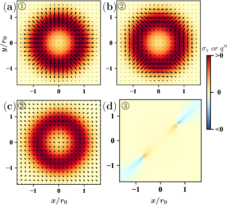
Figure 1: (color online). Spin textures of the ground state of InAs rings, a) with Rashba SOC only, $\hbar g_{1}$ =20.0 nm$\cdot$ meV, b) with Dresselhauss SOC only, $\hbar g_{2}$ = 20.0 nm$\cdot$ meV, c) and with both SOCs, $\hbar g_{1}=7.6$ nm$\cdot$meV, $\hbar g_{2}=12.4$ nm$\cdot$ meV at $B=2.8$T, and d) the spatial distribution of the topological charge $q^{\prime\prime}\left(\mathbf{r}\right)$ of Fig. 1 c). Hereafter, the arrows in the spin texture figures represent the in-plane spin field $\mathbf{\sigma}$ and the background colors represent the $\sigma_{z}\left(\mathbf{r}\right)$, unless otherwise stated. The arrows in Fig. 1 c) are normalized $\mathbf{\sigma}$ field, for $\mathbf{\sigma}\left(\mathbf{r}\right)$ is very small near $\theta=0.25\pi$ and can not be shown clearly. The encircled numbers are explained in the text.

Some typical spin textures in weak magnetic fields, which are similar to those in quantum dots, are indicated in Fig. 1. In Fig. 1(a) we show a vortex with $q=1$, since only the Rashba SOC is present. In Fig. 1 (b) a vortex with $q=-1$ is indicated when only the Dresselhaus SOCs is present. The spin textures are also the same as for the exact solution and the perturbation results discussed in the last section. Fig. 1(c) shows a vortex with $q=1$ if $r<r_{0}$, and $q=-1$ if $r>r_{0}$, when $\hbar g_{1}=7.6$nm$\cdot$ meV, $\hbar g_{2}=12.4$nm$\cdot$meV at $B=2.8$T. In this example, we can see clearly that the topological charge depends on the path of the integral. It is because, there are more than one vortices in the plane. The $q^{\prime\prime}(\mathbf{r})$ is displayed in Fig. 1(d) and its zero points $(-0.8,-0.8),(0.8,0.8)$ and $(0,0)$ correspond to three vortex cores. It is only natural then to calculate the winding number along the routes exactly defined along the ring. Hence, we consider the topological charge to be given by $q^{\prime}$, which is equivalent to $q(r_{0})$, in the case when the ring is narrow.

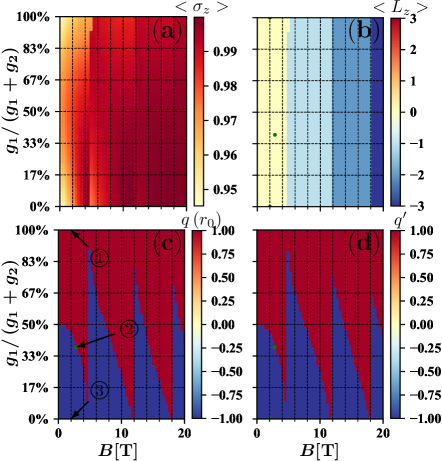
Figure 2: (Color online) The (a) $\left\langle\sigma_{z}\right\rangle$, (b) $\left\langle L_{z}\right\rangle$, (c) $q\left(r_{0}\right)$ and (d) $q^{\prime}$ of the ground state of InAs rings in $B\in$[0, 20]T, $\hbar g_{1}\in$[0, 20] nm$\cdot$ meV and fixed $\hbar g_{1}+\hbar g_{2}$ = 20 nm$\cdot$ meV.

If the electron density is located around $r=r_{0}$, the winding number along the path $r=r_{0}$ is consistent with the overall topological properties. As shown in Fig. 2, there is no major difference between $q\left(r_{0}\right)$ and $q^{\prime}$. The spin textures of the three points marked on Fig. 2 (c) have been given in Fig. 1 (a)-(c).

Just as we found in the 1D ring, the topological charge can be varied periodically with the increase of the magnetic field. Here, the numerical results of the 2D rings also show that the topological features are tunable by adjusting the magnetic field or the SOCs. As expected from the analytical results, the topological charge of the ground state (Fig. 2 (d)), following the change of $l$ which is the quantum number of the angular momentum $\left\langle L_{z}\right\rangle$ (Fig. 2 (b)), is also periodically changed with the magnetic field. This is interesting since the sign change in quantum dots happens at most once in quantum dot hydrogen or helium luo2 . It is because $\left\langle L_{z}\right\rangle$ is varied when the magnetic flux of the ring is increased. Moreover, $\left\langle\sigma_{z}\right\rangle$ (Fig. 2(a)) also changes with the change of $\left\langle L_{z}\right\rangle$, which can be detected by NMR sean . It is worth noting that the sign change of $q^{\prime}$ does not occur exactly at $l-N=\pm\frac{1}{2}$. This is because the charge density in a 2D ring is not all concentrated at $r=r_{0}$, which is slightly biased from the strict 1D results.

IV.2 Current induced by the external magnetic field and the SOCs

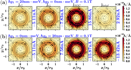
Figure 3: (color online). Persistent current density of the ground states of InAs rings when only one SOC exists: (a) for the Rashba SOC and (b) for the Dresselhaus SOC. The parameters of the ring are indicated in the figures. From left to right, $\mathbf{j}_{z\uparrow}\left(\mathbf{r}\right)$, $\mathbf{j}_{z\downarrow}\left(\mathbf{r}\right)$, $\mathbf{j}_{SOC}\left(\mathbf{r}\right)$ and the total current density $\mathbf{j}_{total}\left(\mathbf{r}\right)$. The currents $I_{total}$ pass through the line $x>$0, $y$=0 (clockwise is positive) are shown on the right side of the figures. The background colors represent the absolute value of the current density.

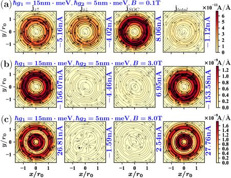
Figure 4: (color online). Current density of the ground states of InAs rings when both of the SOCs are present. (a)-(c) The parameters of the ring are indicated in the figures. The order of the current fields is the same as in Fig. 3. $I_{total}$ pass through the line $x>$0, $y$=0 (clockwise is positive) and is also shown. The colors represent the absolute value of the current density.

In a quantum dot the Hamiltonian is

$$H_{dot}=H_{0}+H_{SOC},$$ (45)

(Eq. (3) but without $H_{r}$). The net current $\left\langle j_{x}\right\rangle=\left\langle j_{y}\right\rangle=0$ since the electrons are trapped locally in the dot. The conservation of the current also requires that the net current vanishes. However, the local current density could be nonzero. We perform the perturbation calculation where $H_{SOC}$ is the perturbation, and are able to obtain the current density. We suppose the Landé $g$ factor of the system $g<0$ (such as in InAs). If there is no Dresselhaus SOC, then $g_{1}\neq 0,g_{2}=0$, and we obtain $\mathbf{j}^{R}=\frac{1}{2}eg_{1}\left(-\sigma_{y}^{R}\left(\mathbf{r}\right),\sigma_{x}^{R}\left(\mathbf{r}\right)\right).$ This means that the current field is perpendicular to the spin field $\mathbf{j}^{R}\cdot\bm{\sigma}=0$. The local current does not vanish. The net current is zero since $\left\langle\sigma_{x,y}\right\rangle=0$.

For the Dresselhaus SOC, $g_{1}=0,g_{2}\neq 0$, and we have $\mathbf{j}^{D}=\frac{1}{2}eg_{2}\left(-\sigma_{x}^{D}\left(\mathbf{r}\right),\sigma_{y}^{D}\left(\mathbf{r}\right)\right)$. The current is not perpendicular to the spin field in this case. We already know that the spin field has topological charge $q=1$ for the dot with Rashba SOC, and $q=-1$ for a dot with Dresselhaus SOC. The vorticity of the spin field is zero, $\bm{\omega}_{s}=\bm{\nabla}\times\bm{\sigma}=0$, if only one SOC is present. However, the vorticity of the current of the Rashba dot $\bm{\omega}_{c}^{R}$ (or $\bm{\omega}_{c}^{D}$ of the Dresselhaus dot) is nonzero. The vorticities of the two different spin-orbit coupled dots are just the opposite in weak magnetic fields $B\rightarrow 0$, $\bm{\omega}_{c}^{D}/g_{2}^{2}=-\bm{\omega}_{c}^{R}/g_{1}^{2}$.

In a quantum ring the results are essentially equivalent to the case of the dots in weak magnetic field. We again employ the 1D model and find that ($g<0$)

$$j^{s}_{x} = -\frac{e}{m^{*}r_{0}^{2}}\xi_{l,s}\sin\theta+s\frac{e}{\pi r_{0}^{2}}\left[g_{1}\left(G_{1s}\sin\theta-G_{2s}\cos\theta\right)\right.$$ (46)

$$+\left.g_{2}\left(G_{1s}\cos\theta-G_{2s}\sin\theta\right)\right],$$

$$j^{s}_{y} = \frac{e}{m^{*}r_{0}^{2}}\xi_{l,s}\cos\theta-s\frac{e}{\pi r_{0}^{2}}\left[g_{1}\left(G_{1s}\cos\theta-G_{2s}\sin\theta\right)\right.$$ (47)

$$+\left.g_{2}\left(G_{1s}\sin\theta-G_{2s}\cos\theta\right)\right],$$

where

$$\xi_{l,s} = \left(l-s\right)G_{1s}^{2}+\left(l+s\right)G_{2s}^{2}-2lG_{1s}G_{2s}\sin 2\theta$$

$$+l-\frac{1}{2}\frac{r_{0}^{2}}{\ell_{B}^{2}}-\frac{1}{2}\frac{r_{0}^{2}}{\ell_{B}^{2}}\left(G_{2s}^{2}+G_{1s}^{2}-2G_{1s}G_{2s}\sin 2\theta\right)$$

with $s=\pm$ corresponding to the case $g<0,g>0$, respectively. The magnetic length is $\ell_{B}=\sqrt{\hbar/(eB)}$.

For simplicity, we consider a ring with the Rashba spin-orbit interaction only ($g_{2}=0$) in a small magnetic field. Then $\ell_{B}\rightarrow\infty$ and $l=0$, so that the current is dominated by the SOC field

$$\mathbf{j}^{R} = \frac{e}{2\pi}\frac{m^{*}g_{1}^{2}}{\hbar r_{0}}(-\sin\theta,\cos\theta).$$ (48)

The ring with Dresselhaus SOC only ($g_{1}=0$) in a small magnetic field gives the current field

$$\mathbf{j}^{D} = \frac{e}{2\pi}\frac{m^{*}g_{2}^{2}}{\hbar r_{0}}(\sin\theta,-\cos\theta).$$ (49)

It is obvious that these two currents are, as in the quantum dots, just the opposite, and the vorticities of the two current fields are also opposite, $\bm{\omega_{c}}^{R}/g_{1}^{2}=-\bm{\omega_{c}}^{D}/g_{2}^{2}$.

The corresponding numerical results of 2D rings with the Rashba SOC and with the Dresselhaus SOC in magnetic fields are displayed in Fig. 3. If $B\rightarrow 0$, the numerical results perfectly agree with the results of the 1D model shown above, $\mathbf{j}_{z\uparrow}\approx 0$, $\mathbf{j}_{SOC}$=$-2\mathbf{j}_{z\downarrow}$, and $\mathbf{j}_{total}$=$0.5\mathbf{j}_{SOC}$, and the vorticity of $\mathbf{j}_{SOC}$ for different SOC is opposite. When the magnetic field is very weak, the direction of the total current is determined by the $\mathbf{j}_{SOC}$ term. When the magnetic field is increased to B=0.1T as shown in Figs. 3 (a) and (b), $\mathbf{j}_{z\uparrow}$ is no longer negligible. Note that the directions of $\mathbf{j}_{z\uparrow}$ and $\mathbf{j}_{z\downarrow}$ are the same and does not depend on the type of SOC, which makes the total currents different in a finite magnetic field (Figs. 3(a) and (b)).

The sign of $\mathbf{j}_{total}$ is easy to reverse when introducing the Dresselhaus SOC (Fig. 4(a)), since the direction of $\mathbf{j}^{D}_{SOC}$ is opposite to the direction of $\mathbf{j}^{R}_{SOC}$. When the magnetic field continues to increase (for instance up to $B=3$T), $\mathbf{j}_{z\uparrow}$ will play a major role (Fig. 4(b)). We also indicate the current field at $B=8$T in Fig. 4(c), where the effect of the SOCs is weakened by the magnetic field, since the spin is more polarized in a stronger magnetic field. The current induced by the SOCs is also weakened, but the total current becomes complex for more than one circles.

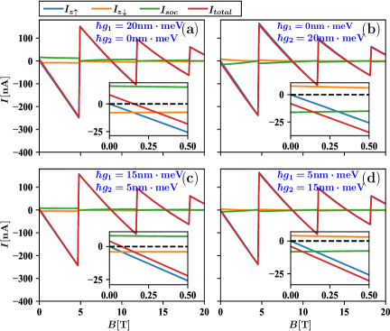
Figure 5: (Color online) In-plane persistent current of the ground state of InAs rings a)-d). The parameters of the SOCs are indicated in the figures.

It is natural to define the current

$$I_{\alpha}=\int\nolimits_{0}^{\infty}\mathbf{j}_{\alpha}\left(x,y=0\right)dx.$$ (50)

The periodic oscillations of $I_{total}$ induced by the AB effect can be found in Fig. 5, which is compatible with the previous works sheng ; janine . Interestingly, $I_{SOC}=-2I_{z\downarrow}$, and if $g_{1}+g_{2}$ is fixed, $I_{z\uparrow}$ for any combination of $g_{1}$ and $g_{2}$ are almost equal. At the points $l-N\approx 0$, $\ I_{z\uparrow}\rightarrow 0.$ Then $I_{SOC}$ plays an important role, which makes it possible to distinguish the type of the SOCs by detecting the direction of the current due to the fact that the direction of $I_{SOC}$ for Rashba and Dresselhaus SOCs are the opposite.

IV.3 Magnetic field induced by the current and spins

The nonzero local current density can induce a magnetic field $\mathbf{B}^{c}$. The steady current in the 2D ring flows along a couple of concentric circles and induces the magnetic field in the three-dimensional (3D) space. In order to calculate the induced magnetic field, we cover the plane of the ring by a square lattice with the lattice constant $b$. According to the Biot-Savart law, on the $i$-th site of the lattice the current induces the magnetic field distributed in the space, which is given by

$$\mathbf{B}^{c}_{i}(\mathbf{r})=\frac{\mu_{0}}{4\pi}\dfrac{b^{2}\mathbf{j}(\mathbf{r^{\prime}}_{i})\times(\mathbf{r-r^{\prime}}_{i})}{|\mathbf{r-r^{\prime}}_{i}|^{3}},$$ (51)

where $\mu_{0}$ is the vacuum permeability, $\mathbf{r}$ is a point in the 3D space, and $\mathbf{r^{\prime}}_{i}$ is the position of the $i-$th site of the lattice. The magnetic field $\mathbf{B}^{c}$ induced by the current is consequently calculated by the summation of the magnetic fields induced by all the sites, $\mathbf{B}^{c}(\mathbf{r})=\sum_{i}\mathbf{B}^{c}_{i}(\mathbf{r})$, once we obtain the full current field. Meanwhile, the spin field also induces a magnetic field $\mathbf{B}^{s}$ in the semiclassical treatment. However, in this case, we need to introduce the $z$ axis into the system, since the spin field is equivalent to the magnetic moment which is induced by the closed current flowing on the plane perpendicular to the 3D spin field.

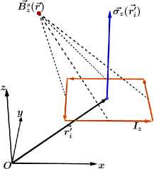
Figure 6: (Color online) The schematic diagram that how the spin field induces an effective magnetic field semi-classically. The $z$ component of the spin field $\sigma_{z}(\mathbf{r^{\prime}}_{i})$ at site $\mathbf{r^{\prime}}_{i}$ is equivalent to the current square (orange) with side length $b$, and the currents induce the magnetic field $\mathbf{B}^{s}_{z}(\mathbf{r})$ in the real space calculated by the Biot-Savart law.

For each component of the spin field $\sigma_{\nu}(\bm{r^{\prime}}_{i})$ at the site $i$, it is equivalent to a constant current along the square coil (with the side length $b\ll\ell$) located in the plane perpendicular to the axis of $\nu$. The constant current $I_{\nu}$ induces a magnetic moment $\mu_{I_{\nu}}$ at $\bm{r^{\prime}}_{i}$, which needs to be equal to the $\nu$ component spin magnetic moment at $\bm{r^{\prime}}_{i}$,

$$\mu_{I_{\nu}}(\mathbf{r^{\prime}}_{i})=I_{\nu}b^{2}=\mu_{B}\int_{b\times b}\psi^{\dagger}\sigma_{\nu}\psi dS,$$ (52)

where the two-dimensional integral covers the area of the $b\times b$ square. When $b$ is very small we can approximately find the current $I_{\nu}=\mu_{B}\psi^{\dagger}\sigma_{\nu}\psi.$ Once the current $I_{\nu}$ is found, we can use the Biot-Savart law to calculate the magnetic field induced by the current along the edge of this $b\times b$ square. The shcematic picture of this process is shown in Fig. 6, where we take the spin field $\sigma_{z}(\mathbf{r}^{\prime}_{i})$ as an example. Then we sum over all the squares covering the area of the spin field to obtain the magnetic field distribution $\mathbf{B}^{s}_{\nu}(\mathbf{r})$. For instance, the magnetic field induced by the $z$ component of the spin magnetic moment is given by

$$\mathbf{B}_{z}^{s}\left(\mathbf{r}\right) = \frac{\mu_{0}}{4\pi}I_{z}b\sum_{i}\left[\frac{\widehat{x}\times\left(\mathbf{r}-\mathbf{r}_{i}^{\prime}+\frac{b\widehat{y}}{2}\right)}{\left|\mathbf{r}-\mathbf{r}_{i}^{\prime}+\frac{b}{2}\widehat{y}\right|^{3}}\right.$$ (53)

$$+\frac{\widehat{y}\times\left(\mathbf{r}-\mathbf{r}_{i}^{\prime}-\frac{b\widehat{x}}{2}\right)}{\left|\mathbf{r}-\mathbf{r}_{i}^{\prime}-\frac{b}{2}\widehat{x}\right|^{3}}+\frac{-\widehat{x}\times\left(\mathbf{r}-\mathbf{r}_{i}^{\prime}-\frac{b}{2}\widehat{y}\right)}{\left|\mathbf{r}-\mathbf{r}_{i}^{\prime}-\frac{b}{2}\widehat{y}\right|^{3}}$$

$$\left.+\frac{-\widehat{y}\times\left(\mathbf{r}-\mathbf{r}_{i}^{\prime}+\frac{b}{2}\widehat{x}\right)}{\left|\mathbf{r}-\mathbf{r}_{i}^{\prime}+\frac{b}{2}\widehat{x}\right|^{3}}\right]$$

In a similar way we can calculate the other two components of the induced magnetic field. Note that for $\sigma_{x,y}$, we need to use the squares in the $y-z$ and $x-z$ planes, respectively. Since $b\ll\ell$ and we do not expand our rings too much in the $z$ direction, it is acceptable that the ring is supposed to have a thickness $b$ which is much smaller than the radius of the ring. The total magnetic field induced by the spin is thus given by $\mathbf{B}^{s}(\mathbf{r})=\Sigma_{\nu}\mathbf{B}^{s}_{\nu}(\mathbf{r})$.

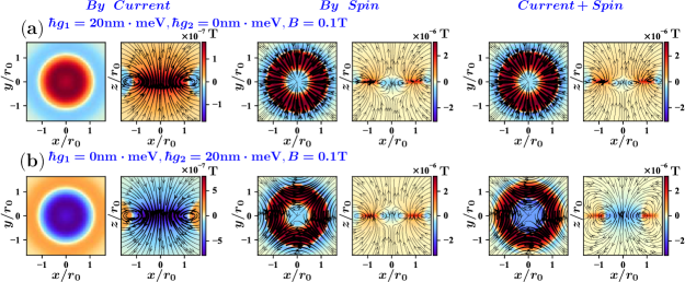
Figure 7: (color online). Magnetic fields induced by the current and the spins with only one SOC. The parameters of the systems in (a) and (b) are the same as those in Figs. 3(a) and (b), respectively. The colors represent the $z$ component of the induced magnetic field, $\left|\mathbf{B}^{c,s}\right|\cdot\text{sgn}\left(B^{c,s}_{z}\right)$. The lines in the first, third and fifth columns are the induced magnetic induction lines on the $xOy$ plane. The second, fourth and the sixth columns indicate the induced magnetic induction lines on the $xOz$ plane.

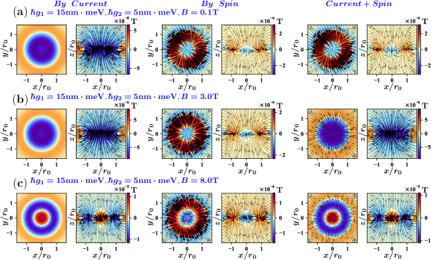
Figure 8: (color online). Magnetic fields induced by the current and the spins, when both of the SOCs are present. The parameters of the systems in (a) to (c) are the same as those in Fig. 4 (a) to (c) respectively. The arrows represent the induced magnetic induction lines. Colors represent $\left|\mathbf{B}^{c,s}\right|\cdot\text{sgn}\left(B^{c,s}_{z}\right)$.

When $B\rightarrow 0$, the direction of the current is opposite for different SOCs, so that the current induced magnetic fields are opposite. But $B^{s}$ is almost the same along the $z$ direction. Hence, $\mathbf{B}^{c}+\mathbf{B}^{s}$ is distinguishable for different type of the SOC (Fig. 7(a) for the Rashba SOC and Fig. 7(b) for the Dresselhuas SOC), which can be utilized in indirectly determining topological charge of the spin textures, if the induced magnetic field can be detected. Since the direct measurement of the topology of the spin field is very difficult, we propose here another indirect measurement other than detecting $\langle\sigma_{z}\rangle$. The current is strictly located on the 2D surface, so no in-plane magnetic field is induced by the current. On the other hand, the spin vortices induce the in-plane magnetic moment due to the existence of the SOCs as shown in Fig. 7 and Fig. 8.

When both of the SOCs are present, examples of the magnetic induction lines distributions are also indicated in Fig. 8. In a small external magnetic field, $\left|\mathbf{B}^{c}\right|\propto\left|g_{1}^{2}-g_{2}^{2}\right|$. But it can be increased significantly with the increase of the external magnetic field. According to Eqs. (46), (47) and (51), the current varies linearly with the external magnetic field, so that the current induced magnetic is sensitive to the external magnetic field. Consequently, from $B=0.1$T to $B=8$T, $|\mathbf{B}^{c}|$ increases by two orders of magnitude. In contrast, the spin magnetic moment does not vary much $\left|\mathbf{B}^{s}\right|\propto\frac{1}{\hbar\omega r_{0}^{2}}$, since the magnitude of the spin field in Eqs. (37) and (38) is not strongly related to the magnetic field. Therefore, in a strong magnetic field, the total induced magnetic field above the center of the ring points down (Figs. 8(b) and (c)) due to the large cyclotron motion of the charge.

These findings in this subsection help us to find another way to measure the topological charge of the in-plane field indirectly in a weak magnetic field, i.e., to determine the direction of the total induced magnetic field above the center of the ring as shown in Fig. 7.

V Size effect and the limitations of the 1D model

V.1 The spin fields in different size of the ring

The full Hamiltonian is difficult to solve analytically. However, in some cases, we can have analytical approaches that are very close to the real situation. The 2D Hamiltonian can be written as

$$H=\frac{1}{2m^{*}}\left[\mathbf{p}+e\left(\mathbf{A+A}^{R}+\mathbf{A}^{D}\right)\right]^{2}+V(\mathbf{r}),$$ (54)

where $V(\mathbf{r})$ is the confinement potential and the SOCs are written in the form of effective vector potentials $\mathbf{A}^{R}=\frac{mg_{1}}{e}\left(-\sigma_{y},\sigma_{x}\right),\mathbf{A}^{D}=\frac{mg_{2}}{e}\left(-\sigma_{x},\sigma_{y}\right),$ for the Rashba and Dresselhaus SOCs, respectively. When the SOCs are weak, the wave function is given approximately by

$$\psi\left(\mathbf{r}\right)\approx\exp\left[-i\frac{e}{\hbar}\left(\mathbf{A}^{R}+\mathbf{A}^{D}\right)\mathbf{\cdot r}\right]\psi_{0}\left(\mathbf{r}\right),$$ (55)

where $\psi_{0}$ is the wave function of the Hamiltonian without the SOC. In an InAs quantum dot, $\psi_{0}=\left(\begin{array}[]{cc}\psi_{n,l}&0\\ \end{array}\right)^{T}$ is the wave function of the Fock-Darwin basis given by Eq. (6). We can obtain that the results of the special case that $g_{1}=g_{2}$ is exactly the same as found in Ref. luo1 .

For simplicity and without loss of generality, we choose $\psi_{0}\left(\mathbf{r}\right)=\left(\begin{array}[]{cc}f(\mathbf{r})&0\end{array}\right)^{T}$ where $f$ is the wave function of the quantum ring without the SOC. We can then readily obtain

$$\psi\left(\mathbf{r}\right)=f(\mathbf{r})\left(\begin{array}[]{c}\cos\Theta\\ \frac{-\beta_{1}e^{i\theta}+i\beta_{2}e^{-i\theta}}{\Theta}\sin\Theta\end{array}\right)\allowbreak,$$ (56)

where $\beta_{1,2}=g_{1,2}m^{\ast}r/\hbar$ should be smaller than unity, and $\Theta=\sqrt{\beta_{1}^{2}-2\left(\sin 2\theta\right)\beta_{1}\beta_{2}+\beta_{2}^{2}}$. The spin fields are consequently

$$\sigma_{x}\left(r,\theta\right) = -|f|^{2}\frac{\sin 2\Theta}{\Theta}\left(\beta_{1}\cos\theta-\beta_{2}\sin\theta\right),$$ (57)

$$\sigma_{y}\left(r,\theta\right) = |f|^{2}\frac{\sin 2\Theta}{\Theta}\left(\beta_{2}\cos\theta-\beta_{1}\sin\theta\right),$$ (58)

$$\sigma_{z}\left(r,\theta\right) = |f|^{2}\cos 2\Theta.$$ (59)

If the system without SOC has rotational symmetry, i.e. $|f|$ is independent of $\theta$, the spin field can be simplified. If only the Rashba SOC is present, then $\beta_{1}\neq 0,\beta_{2}=0,$ we have $\mathbf{\sigma}\left(\theta\right)\propto\left(-\sin 2\beta_{1}\cos\theta,-\sin 2\beta_{1}\sin\theta,\cos 2\beta_{1}\right)$ with topological charge $q=1$, which is compatible with the perturbation calculations. If $g_{1}$ or $r_{0}$ is small, then $\sin 2\beta_{1},\cos 2\beta_{1}>0$, we can find that the in-plane spin vector $\left(-\sin 2\beta_{1}\cos\theta,-\sin 2\beta_{1}\sin\theta\right)$ all points to the center and $\sigma_{z}(\theta)>0$. When $\beta_{1}>\pi/4$, $\cos 2\beta_{1}$ could be negative, then $\sigma_{z}(\theta)$ rotate to be negative. If $g_{1}$ or $r_{0}$ continues to increase then the spin vector rotates along the tangential line of the ring. However, if $g_{1}$ or $r_{0}$ increases too much, the wave function obtained in Eq. (55) is no longer correct. Only the numerical results in the next section are reliable.

In the similar manner, if only the Dresselhaus SOC is present, then we find $\mathbf{\sigma}^{D}\propto\left(\sin 2\beta_{2}\sin\theta,\sin 2\beta_{2}\cos\theta,\cos 2\beta_{2}\right)$ with $q=-1$. The results are compatible with the quantum dot cases. If $g_{2}$ or $r_{0}$ increases, then the spin vector also rotates. The analytical solution of the 1D ring refers to the SOCs can be found in Ref. sheng ; arxiv . However, no rotation of $\sigma_{z}(r)$ was found in the 1D model there. We shall see from our numerical works that the rotation of $\sigma_{z}(r)$ in a 2D ring is possible for the Rashba and the Dresselhaus cases. The numerical results are beyond the perturbation calculations where the SOCs and the radius ($\beta_{1,2}$) are treated as the small quantities, and are always reliable.

V.2 Numerical results

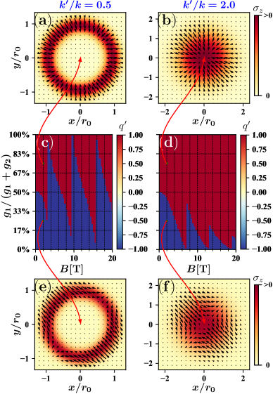
Figure 9: (Color online) The spin textures, density profiles and the topological charges of a narrow ring [(a), (c), (e)], and a wide ring [(b), (d), (f)], respectively.

As discussed above, the spin rotates when $\beta_{1,2}$ increases. There are two possible ways to tune $\beta_{1,2}$: Firstly, we can increase the strength of the Rashba SOC which can be achieved by increasing the potential of the gate Rash01 ; Rash03 ; Rash04 ; Rash05 . Secondly, the radius can also be increased. In this subsection, We would like to explore how the width and the radius of the ring affects the spin textures of the quantum ring.

For convenience, we define the ratio of the ring width $\sqrt{\frac{\hbar}{m^{*}\omega}}$ to the radius $r_{0}$, $k^{\prime}(\hbar\omega,r_{0})=\sqrt{\frac{\hbar}{m^{\ast}\omega r_{0}^{2}}}$. If $k^{\prime}$ is small, the ring is effectively narrow and the radius is large, while the ring is like a dot if $k^{\prime}$ is large. We choose the example $r_{0}=15$ nm, $\hbar\omega=40$ meV in an InAs ring as the reference, of which the ratio is $k\equiv k^{\prime}(40,15)=0.449$. We then explore how the spin textures evolves by changing this ratio.

For the ratio $k^{\prime}=k$, the topological charges varying in the external magnetic fields has been studied in Fig. 2. In Figs. 9(a), (c), (e), spin textures, density profiles and the topological charge $q^{\prime}$ are displayed when the width-radius ratio is $k^{\prime}=k/2$, which corresponds to a big narrow ring. In Figs. 9(b), (d), (f), those quantities are displayed when the ratio is $k^{\prime}=2k$, corresponding to a wide ring which is similar to a quantum dot. The periodic topological effect due to the Aharonov-Bohm effect is still existing. However, in a wide ring, there is no topological transition when $g_{1}>g_{2}$, which is similar to the case of quantum dot.

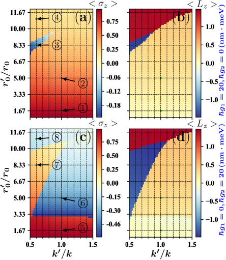
Figure 10: (color online). The $\left\langle\sigma_{z}\right\rangle$ and $\left\langle L_{z}\right\rangle$ of the ground state of InAs rings with $k^{\prime}/k\in$[0.5, 1.5], $r_{0}^{\prime}/r_{0}\in$[0.5, 12.0]. The SOCs are: (a) and (b) $\hbar g_{1}$ = 20 nm$\cdot$ meV, (c) and (d) $\hbar g_{2}$ = 20 nm$\cdot$ meV.

We further study how the ratio affects the observable quantities such as $\langle\sigma_{z}\rangle$ and $\langle L_{z}\rangle$. We utilize the 1D model in the perturbation theory. We find that the perturbative ground state may vary when the radius is increased for a small magnetic field. The energy of the unperturbed ground state without SOC is $E_{0,+}<E_{0,-}$ given by Eq. (33). However, with the SOC, the real ground state would be spin flipped, as in a quantum dot luo1 . Generally, the flip condition is given by $E_{0,+}+E_{0,+}^{(2)}>E_{0,-}+E_{0,-}^{(2)}$. In this case, the ground state will be altered to the spin-down state and the $\langle\sigma_{z}\rangle$ is flipped, which requires that the radius satisfies ($g<0$)

$$r_{0}>\frac{\hbar}{m^{\ast}}\sqrt{\frac{-0.5\beta_{3}}{g_{2}^{2}\left(1-\beta_{3}\right)-g_{1}^{2}\left(1+\beta_{3}\right)}}$$ (60)

when the magnetic field approaches zero, where $\beta_{3}=gm^{*}$.

If there is only the Dresselhaus SOC present, then we find that $r_{0}>\frac{\hbar}{g_{2}m^{*}}\sqrt{\frac{-\beta_{3}}{2(1-\beta_{3})}}$. We use the condition in Fig. 10 where we fixed the quantum flux and $N=\frac{2eBr_{0}}{\hbar}=0.34$, it results in $r_{0}>39$ nm. This agrees with the lowest transition line in Fig. 10(c) where the transition line of $\langle\sigma_{z}\rangle$ is $r^{\prime}_{0}\approx 45$ nm. We note that for the ring with Rashba SOC only, such a spin flipping also exists when the radius of the ring increases, but for $\beta_{3}<-1$. We note that for InAs, $\beta_{3}=-0.588>-1$, so that this spin flipping can not be found in the Rashba spin-orbit coupled 1D InAs ring. But it is possible for some another materials with $g<0$, which is different from the case of quantum dot. In quantum dots, the spin flipping is only possible by the Dresselhaus SOC for a negative Landé $g$ material, and the Rashba SOC can not flip the spin unless $g>0$ luo1 .

Surprisingly, we also numerically find the spin flipping happening in a Rashba spin-orbit coupled 2D InAs ring with $g_{1}\neq 0,g_{2}=0$ in Fig. 10(a). It is completely different from the case of the InAs quantum dot luo1 where only the Dresselhaus SOC can flip $\langle\sigma_{z}\rangle$ in a large dot. Moreover, we find another spin flipping region in the Dresselhaus spin-orbit coupled 2D ring, as the triangle region shown in Fig. 10(c). Those spin flips can not be explained by the 1D model, where the radial differential is a constant $\partial/\partial r\rightarrow 1/r_{0}$. However, in a 2D system this term is never a constant. Only the 2D model stated in the last subsection can qualitatively explain the rotation, i.e. $\cos 2\beta_{1,2}<0$. However, these abnormal spin flip regions do not correspond exactly to $\beta_{1,2}<\pi/4$, since the wave function obtained in Eq. (55) is not accurate when the radius is large.

In Fig. 10, the flipping of $\langle\sigma_{z}\rangle$ (and $\langle L_{z}\rangle$) in the rings with Rashba SOC or with Dresselhaus SOC are shown, which may be observed in NMR experiments. The spin textures of some cases marked in Fig. 10, ① to ⑧ are plotted in Fig. 11. In the case ⑥ shown in Fig. 11(f) where the spin flipping is induced by the energy alternating $E_{0,+}+E_{0,+}^{(2)}>E_{0,-}+E_{0,-}^{(2)}$, so that all the $\sigma_{z}(\mathbf{r})$ points down. However in Figs. 11(c), (d), (g) and (h), with the increase of the radius we can clearly observe that $\langle\sigma_{z}\rangle$ changes its sign by the size effect, which can not be explained by the 1D model.

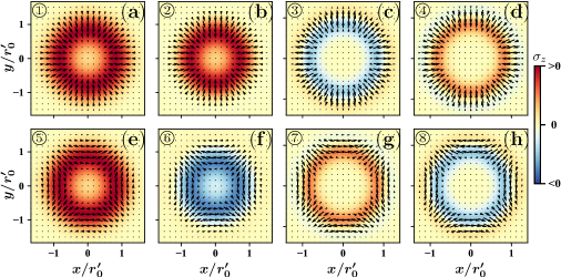
Figure 11: (color online) Spin textures of the ground states of InAs rings (① to ⑧) marked in Fig. 10.

VI Conclusion

In summary, we have studied the 1D ideal model if the SOCs are weak and can be treated as perturbation. We analyze the system in the perturbation theory. We then show that the winding number (topological charge) of the InAs quantum rings can be tuned by both electric and magnetic fields in the presence of both Rashba and Dresselhaus SOCs. Compared to the quantum dots, quantum rings exhibit several new properties, the major one is that that its winding number periodically changes the sign with the magnetic field due to the AB effect.

The current induced by magnetic field and by the SOCs reveal nonzero persistent current $I_{total}$. $I_{SOC}$ plays an important role which makes it possible to distinguish the type of SOC by adjusting the current direction when $l-N\approx 0$ in a weak magnetic field. Consequently, the magnetic fields induced by these currents and the spin field are also numerically calculated and we find that it may be used as a means of measuring the topology of the spin textures in a weak external magnetic field. Some of the spin rotations with the increase of the radius can be found only in the 2D model, as the 1D model is inadequate for the large ring radius. The size effect can be observed by changing the ring’s radius $r_{0}$ and the width, if the strength of the SOC is difficult to tune. The direction of the spin field could be changed with the increase of $r_{0}$, when the width is narrow relative to the radius. With only the Rashba SOC ithe spin direction cannot be changed in InAs quantum dots, but it can be changed in quantum ring by increasing $r_{0}$. With Dresselhaus SOC only, spin direction changes more than once in the quantum rings when the radius is increased. These findings pave the way to control the topological features of the system in spintronics Zutic ; Smejkal and may be useful in quantum computation qbit . It also leads to the findings of the transport properties when the quantum ring is designed as a transport device peng .

VII Acknowledgement

This work has been supported by the NSF-China under Grant No. 11804396. F.O. acknowledges financial support by the NSF-China under Grant No. 51272291, the Distinguished Young Scholar Foundation of Hunan Province (Grant No. 2015JJ1020), and the CSU Research Fund for Sheng-hua scholars (Grant No. 502033019).

References

- (1) M. Z. Hasan, and C. L. Kane, Rev. Mod. Phys. 82, 3045 (2010).
- (2) X. L. Qi and S. C. Zhang, Rev. Mod. Phys. 83, 1057 (2011).
- (3) N. Nagaosa and Y. Tokura, Nature Nanotech. 8, 899 (2013).
- (4) S. Mühlbauer, B. Binz, F. Jonietz, C. Pfleiderer, A. Rosch, A. Neubauer, R. Georgii, P. Böni, Science 323, 915-919 (2009).
- (5) X. Z. Yu, Y. Onose, N. Kanazawa, J. H. Park, J. H. Han, Y. Matsui, N. Nagaosa, and Y. Tokura, Nature 465, 901-904 (2010).
- (6) Z. F. Ezawa, Quantum Hall Effects: Field Theoretical Approach and Related Topics (World Scientific, 2000).
- (7) Wenchen Luo and Tapash Chakraborty, Phys. Rev. B 92, 155123 (2015).
- (8) D.S.L. Abergel, V. Apalkov, J. Berashevich, K. Ziegler, and T. Chakraborty, Adv. Phys. 59, 261 (2010).
- (9) X.F. Wang and T. Chakraborty, Phys. Rev. B 81, 081402 (2010); D.S.L. Abergel and T. Chakraborty, Nanotechnology 22, 015203 (2010).
- (10) R. Côté, Wenchen Luo, Branko Petrov, Yafis Barlas, and A. H. MacDonald, Phys. Rev. B 82, 245307 (2010); R. Côté, J. P. Fouquet, and Wenchen Luo, Phys. Rev. B 84, 235301 (2011).
- (11) P.A. Maksym, and T. Chakraborty, Phys. Rev. Lett. 65, 108 (1990).
- (12) T. Chakraborty, Quantum Dots (Elsevier, Amsterdam 1999).
- (13) D. Bimberg, M. Grundmann, and N. N. Ledentsov, Quantum Dot Heterostructures (John Wiley and Sons, Chichester, 1999).
- (14) L. P. Kouwenhoven, D. G. Austing, and S. Tarucha, Rep. Prog. Phys. 64, 701-736 (2001).
- (15) R. Hanson, L. P. Kouwenhoven, J. R. Petta, S. Tarucha, and L. M. K. Vandersypen, Rev. Mod. Phys. 79, 1217 (2007).
- (16) C. Kloeffel, and D. Loss, Annu. Rev. Condens. Matter Phys. 4, 51 (2013).
- (17) Tie-Feng Fang, Ai-Min Guo, and Qing-Feng Sun, Phys. Rev. B 97, 235115 (2018); Gao-Yang Li, Tie-Feng Fang, Ai-Min Guo, and Qing-Feng Sun, Phys. Rev. B 100, 115115 (2019).
- (18) Wenchen Luo, Amin Naseri, Jesko Sirker, and T. Chakraborty, Sci. Rep. 9, 672 (2019).
- (19) Wenchen Luo and T. Chakraborty, Phys. Rev. B 100, 085309 (2019).
- (20) S.L. Zhang, G. van der Laan, and T. Hesjedal, Nature Commun. 8, 14619 (2017).
- (21) T. Chakraborty, and P. Pietiläinen, Phys. Rev. B 52, 1932 (1995); Hong-Yi Chen, P. Pietiläinen, and Tapash Chakraborty, Phys. Rev. B 78, 073407 (2008); T. Chakraborty, A. Manaselyan, and M. Barseghyan, J. Phys.:Condens. Matter 29, 215301 (2017).
- (22) P. Lucignano, D. Giuliano, and A. Tagliacozzo, Phys. Rev. B 76, 045324 (2007).
- (23) T. Chakraborty, A. Manaselyan, and M. Berseghyan, in Physics of Quantum Rings (Springer, Berlin 2018), edited by V.M. Fomin.
- (24) Aram Manaselyan, Wenchen Luo, Daniel Braak and Tapash Chakraborty, Scientific Reports 9, 9244 (2019).
- (25) J. S. Sheng and Kai Chang, Phys. Rev. B 74, 235315 (2006).
- (26) F. E. Meijer, A. F. Morpurgo, and T. M. Klapwijk, Phys. Rev. B 66, 033107 (2002).
- (27) Janine Splettstoesser, Michele Governale, and Ulrich Zülicke, Phys. Rev. B 68, 165341 (2003).
- (28) J. M. Lia and P. I. Tamborenea, arXiv:1905.00878v1 (2019).
- (29) J. Nitta, T. Akazaki, H. Takayanagi, and T. Enoki, Phys. Rev. Lett. 78, 1335 (1997).
- (30) C. R. Ast, D. Pacilé, L. Moreschini, M. C. Falub, M. Papagno, K. Kern, M. Grioni, J. Henk, A. Ernst, S. Ostanin, and P. Bruno, Phys. Rev. B 77, 081407(R) (2008).
- (31) Y. Kanai, R. S. Deacon, S. Takahashi, A. Oiwa, K. Yoshida, K. Shibata, K. Hirakawa, Y. Tokura, and S. Tarucha, Nat. Nanotechnol. 6, 511 (2011).
- (32) M. P. Nowak, B. Szafran, F. M. Peeters, B. Partoens, and W. J. Pasek, Phys. Rev. B 83, 245324 (2011).
- (33) A.E. Dementyev, P. Khandelwal, N. N. Kuzma, S.E. Barrett, L. N. Pfeiffer, K. W. West, Solid State Comm. 119, 217 (2001); N. N. Kuzma, P. Khandelwal, S. E. Barrett, L. N. Pfeiffer, K. W. West, Science 281, 686 (1998); S. E. Barrett, G. Dabbagh, L. N. Pfeiffer, K. W. West, and R. Tycko, Phys. Rev. Lett. 74, 5112 (1995).
- (34) I. Zutic, J. Fabian, and S. Das Sarma, Rev. Mod. Phys. 76, 323 (2004).
- (35) L. Smejkal, Y. Mokrousov, Binghai Yan, and A.H. MacDonald, Nat. Phys. 14, 242 (2018).
- (36) A. Kregar, J. H. Jefferson amd A. Rams̆ak, Phys. Rev. B 93, 075432 (2016).
- (37) Shenglin Peng, Wenchen Luo, Fangping Ouyang, Ai-Min Guo, Jian Sun and Tapash Chakraborty, unpublished.