Quasi-Monte Carlo sampling for machine-learning partial differential equations
Abstract
Solving partial differential equations in high dimensions by deep neural network has brought significant attentions in recent years. In many scenarios, the loss function is defined as an integral over a high-dimensional domain. Monte-Carlo method, together with the deep neural network, is used to overcome the curse of dimensionality, while classical methods fail. Often, a deep neural network outperforms classical numerical methods in terms of both accuracy and efficiency. In this paper, we propose to use quasi-Monte Carlo sampling, instead of Monte-Carlo method to approximate the loss function. To demonstrate the idea, we conduct numerical experiments in the framework of deep Ritz method proposed by Weinan E and Bing Yu [1]. For the same accuracy requirement, it is observed that quasi-Monte Carlo sampling reduces the size of training data set by more than two orders of magnitude compared to that of MC method. Under some assumptions, we prove that quasi-Monte Carlo sampling together with the deep neural network generates a convergent series with rate proportional to the approximation accuracy of quasi-Monte Carlo method for numerical integration. Numerically the fitted convergence rate is a bit smaller, but the proposed approach always outperforms Monte Carlo method. It is worth mentioning that the convergence analysis is generic whenever a loss function is approximated by the quasi-Monte Carlo method, although observations here are based on deep Ritz method.
Keywords: Quasi-Monte Carlo sampling; Deep Ritz method; Loss function; Convergence analysis
AMS subject classifications: 35J25, 65D30, 65N99
1 Introduction
Deep neural networks (DNNs) have had great success in text classification, computer vision, natural language processing and other data-driven applications (see, e.g., [2, 3, 4, 5, 6]). Recently, DNNs have been applied to the field of numerical analysis and scientific computing, with the emphasis on solving high-dimensional partial differential equations (PDEs) (see, e.g., [1, 7, 8, 9]), which are widely used in physics and finance. Notable examples include Schrödinger equation in the quantum many-body problem [10, 11], Hamilton-Jacobi-Bellman equation in stochastic optimal control [7, 12], and nonlinear Black-Scholes equation for pricing financial derivatives [13, 14].
Classical numerical methods, such as finite difference method [15] and finite element method [16], share the similarity that the approximation stencil has compact support, resulting in the sparsity of stiffness matrix (or Hessian in the nonlinear case). Advantages of these methods are obvious for low dimensional PDEs (the dimension ). However, the number of unknowns grows exponentially as increases and classical methods run into the curse of dimensionality. In another line, spectral method [17] uses basis functions without compact support and thus sacrifices the sparsity, but often has the exponential accuracy. However, the number of modes used in the spectral method also grows exponentially as increases. Sparse grid method [18, 19] mitigates the aforementioned situation to some extent ( typically). Therefore, high-dimensional PDEs are far out of the capability of classical methods.
The popularity of DNNs in scientific computing results from its ability to approximate a high-dimensional function without the curse of dimensionality. To illustrate this, we focus on methods in which the loss function is defined as an integral over a bounded domain in high dimensions; see the deep Ritz method [1] and the deep Galerkin method [20] for example. The success of DNNs relies on composition of functions without compact support and sampling strategy for approximating the high-dimensional integral. It is known that the choice of approximate functions in DNNs is of particular importance. For example, in the current work, the approximate function in one block of DNN consists of two linear transformations, two nonlinear activation functions, and one shortcut connection. Besides, since the network architecture is chosen a priori, thus the number of parameters can be independent of or only grows linearly as increases. On the other hand, only a fixed number of samples (or at most linear growth) is used to approximate the high-dimensional integral. Altogether, DNNs can overcome the curse of dimensionality when solving high-dimensional PDEs. In [21], the above step of numerical quadrature is viewed as approximating the expected risk by its empirical risk using Monte Carlo (MC) method. Consequently, the full gradient of the loss function is approximated by a finite number of samples and the stochastic gradient descent (SGD) method is used to find the optimal set of parameters in the network. It is shown that such a procedure converges under some assumptions [21].
From the perspective of numerical analysis, using i.i.d. random points, MC method approximates an integral with error [22]. It is also known that using carefully chosen (deterministic) points, quasi-Monte Carlo (QMC) method approximates an integral with error and the logarithmic factor can be removed under some assumptions [23, 24, 25, 26]. Therefore, it is natural to replace MC method by QMC method in the community of machine learning. One example is the usage of QMC method in variational inference and QMC method has been proved to perform better than MC method [27]. Another example is the usage of QMC sampling in the stage of data generation for training DNNs; see an application in organic semiconductors [28]. In this work, we consider another application of QMC method, i.e., approximation of the high-dimensional integral in machine-learning PDEs.
In order to demonstrate the advantages of QMC method, we take deep Ritz method [1] as an example. Results obtained here shall be applicable to other methods, like deep Galerkin method [20], where a high-dimensional integral is defined as the loss function. Briefly speaking, deep Ritz method solves a variational problem coming from a high-dimensional PDE using a deep neural network with residual connection. Data are drawn randomly over the high-dimensional domain to train the parameters of the neural network. All numerical observations in the current work are based on deep Ritz method. In deep Galerkin method, the loss function contains not only the volume integral over the high-dimensional domain but also penalty terms for boundary conditions and initial conditions. We also demonstrate the advantage of QMC method in deep Ritz method when the penalty term is present. Theoretically, under certain assumptions, we prove a convergence result of the SGD method with respect to both the iteration number and the size of training data set.
2 Quasi-Monte Carlo sampling for deep Ritz method
For completeness, we first introduce deep Ritz method. The basic idea is to solve a variational problem associated to a PDE using DNNs. The training data points are chosen randomly over the given domain using MC method. SGD method is then used to find an optimal solution. In the current work, QMC method is employed to replace MC method and the other components are remained almost the same. For consistency, we use superscripts for indices of sampling points and subscripts for coordinates of a vector throughout the paper.
2.1 Loss function
We take the variational problem associated to the Poisson equation [29] as an example
| (1) |
where the loss function (objective function) reads as
| (2) |
and the set of trial functions is of infinite dimension. Here is a given function, representing the external force to the system and is a bounded domain in .
When the solution of a PDE is approximated by a neural network , i.e., is restricted to a finite-dimensional space, our goal is to find the optimal set of parameters in the neural network, denoted by , such that
| (3) |
is minimized. Numerically, a quadrature scheme is needed and the above objective function is approximated by
| (4) |
with sampling points which will be specified in §2.3.
2.2 Trail function and network architecture
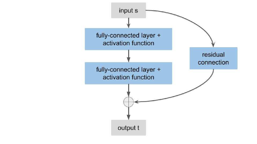
The neural network we use here is stacked by several blocks with each containing two linear transformations, two activation functions and one shortcut connection. The -th block can be formulated as
| (5) |
Here is the input, is the output, weights and is the activation function. Figure 1 demonstrates one block of the network.
To balance simplicity and accuracy, we use the following swish function
| (6) |
as the activation function [30], which is different from the one used in [1].
The last term on the right-hand side of (5) is called the shortcut connection or residual connection. Benefits of using it are [31]:
-
1)
It can solve the notorious problem of vanishing/exploding gradient automatically;
-
2)
Without adding any parameters or computational complexity, the shortcut connection performing as an Identity mapping can resolve the degradation issue (with the network depth increasing, accuracy gets saturated and then degrades rapidly).
With these components, the fully connected -layer network can be expressed as
| (7) |
where denotes the set of parameters in the network. Since the input in the first block is in , not in , we need to apply a linear transformation on before putting it into the network structure. Having , we obtain by
| (8) |
where . Note that the parameters and in (8) also need to be trained.
To make (1) - (2) have a unique solution, a boundary condition has to be imposed. Consider the inhomogeneous Dirichlet boundary condition for example
| (9) |
One way to implement it is to select trail functions that satisfy the boundary condition and thus have to be problem-dependent. To avoid this, we build trail functions of the form
| (10) |
where by choice when and when . Therefore, satisfies the boundary condition automatically. For Neumann boundary condition, however, we have to add a penalty term into the loss function; see (22) in §3.2 for example.
2.3 Sampling strategies
The loss function is defined over a high-dimensional domain, thus only a fixed size of points (mini-batch ) is allowed to approximate the integral. Due to the curse of dimensionality, standard quadrature rules may run into the risk where the integrand is minimized on fixed points but the functional itself is far away from being minimized [1]. Therefore, points are chosen randomly and the approximation accuracy is of [22]. For stochastic problems, from the perspective of sampling strategies, it is well known that QMC method performs much better with the same size of sampling point [32, 33, 34]. We briefly review both methods here.
Consider () for convenience and let be an integrable function in
| (11) |
which is approximated by points of the form
| (12) |
Let being the prescribed sampling points. In MC method, these points are chosen randomly and independently from the uniform distribution in . There exists a probabilistic error (root mean square error) estimate for MC method
where is the variance of of the form
It is easy to check that MC method is unbiased, i.e., . The variance of MC method is
In QMC method, however, sampling points are chosen in a deterministic way to approximate the integral with the best approximation accuracy; see for example [23, 24, 25, 26]. The deterministic feature of QMC method leads to a guaranteed error bounds and faster convergence rate for smooth integral functions. More explicitly, an upper bound of the deterministic error, known as Koksma-Hlawka error bound [24], is
| (13) |
Here variation is defined as
where is the variation in sense of Vitali applied to the restriction of to the space of dimension . Precisely, let be the alternative sum of values at the edges of sub-interval when is a partition of , we give the definition of the variation in sense of Vitali as
is defined to measure the discrepancy of the set as
where . Note that the error bound in (13) is controlled by this discrepancy and if and only if the sequence is equi-distributed. A sequence is said to be a low-discrepancy sequence if , the best-known result for infinite sequences. Therefore, QMC method converges much faster than MC method. Practically, the commonly used Sobol sequence is one of the low-discrepancy sequences [35, 26].
2.4 Stochastic gradient descent method
In deep Ritz method, we use the SGD method to find the optimal set of parameters. The SGD method finds the optimal solution in an iterative way with the -th iteration of the form
| (14) |
where is a stochastic vector
| (15) |
obtained by a sampling strategy, is a sampling point, and is the stepsize. Practically, we use ADAM [36] to accelerate the training process for both MC sampling and QMC sampling.
3 Numerical results
Now we are ready to apply QMC sampling strategy to train the network structure of deep Ritz method in §2.2. For Dirichlet problems and some special Neumann problems, we do not need penalty terms on the boundary. However, for general Neumann problems, a penalty term must be added to the loss function and thus we have to approximate this term by sampling on the boundary. No matter in which case, numerically QMC method always performs better than MC method. We use the relative error for quantitative comparison in all examples
| (16) |
3.1 Dirichlet problem
Consider the Poisson equation over
| (17) |
The exact solution is . We construct the network in the form of
| (18) |
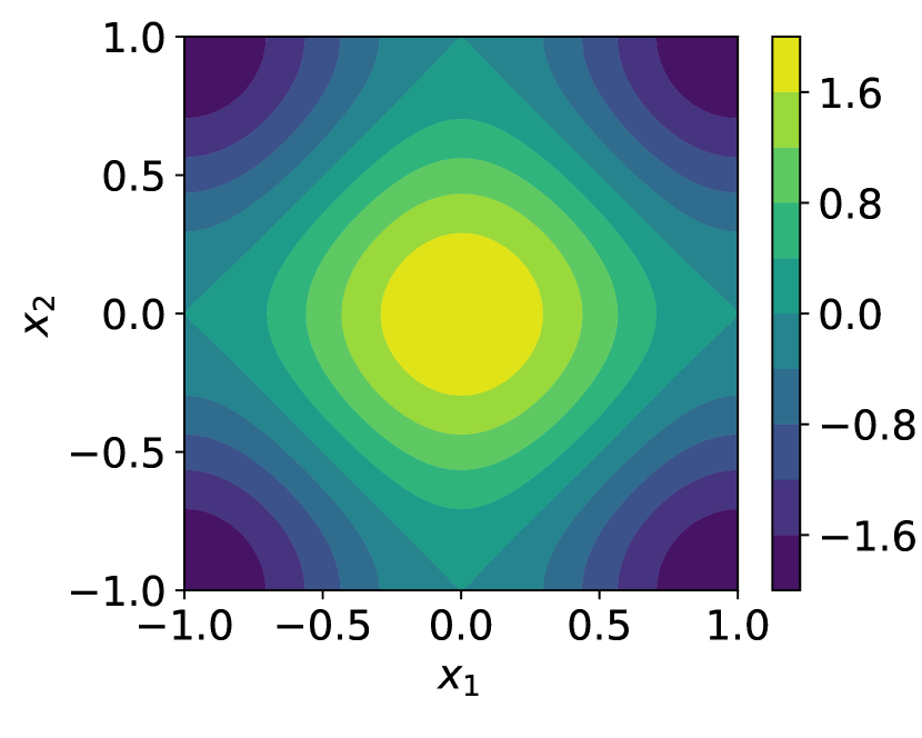
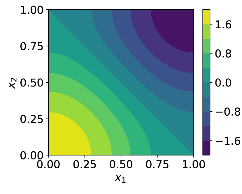
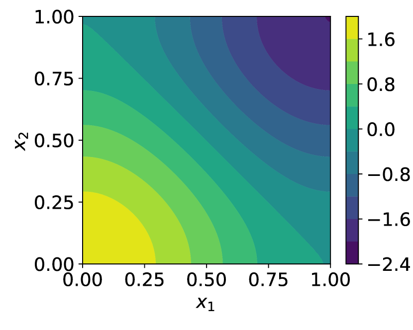
It is easy to verify that on the boundary, satisfying the structure defined in (10). Figure 2 plots exact and trained solutions to (17) in 2D and qualitative agreement is observed.

Detailed setup of the neural network used for Dirichlet problem in different dimensions is recorded in Table 1.
| Dimension | Blocks Num | Parameters | |
|---|---|---|---|
| 2 | 3 | 8 | 465 |
| 4 | 4 | 16 | 2274 |
| 8 | 4 | 20 | 3561 |
| 16 | 4 | 48 | 19681 |
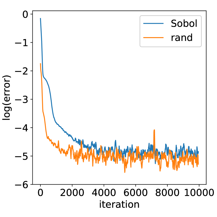
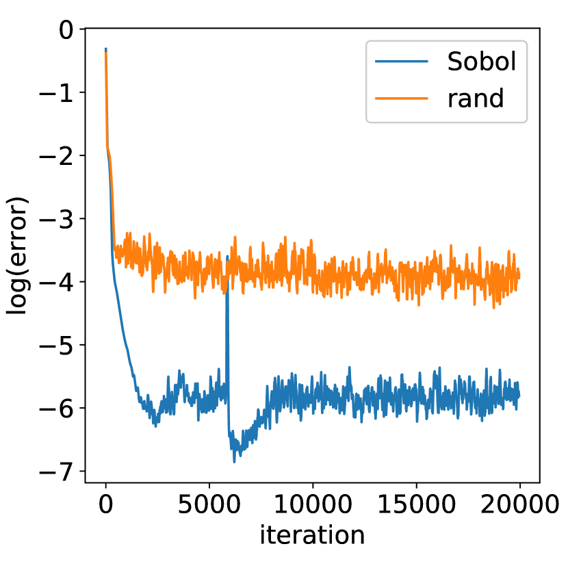
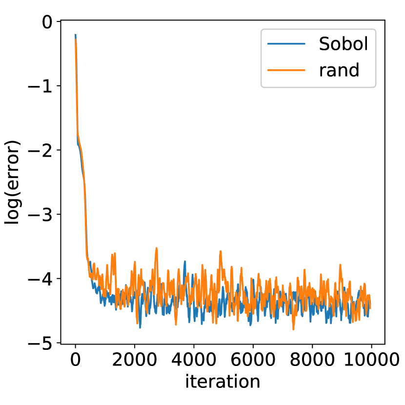
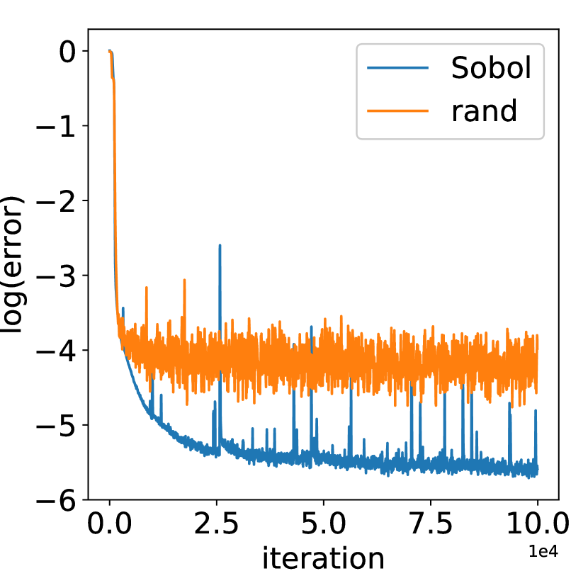
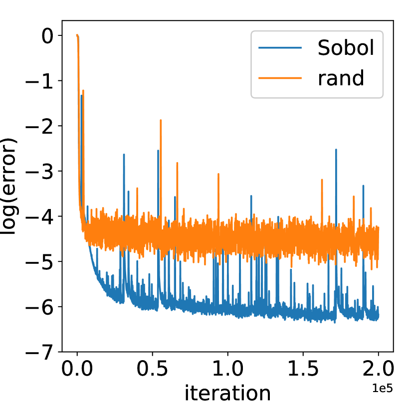
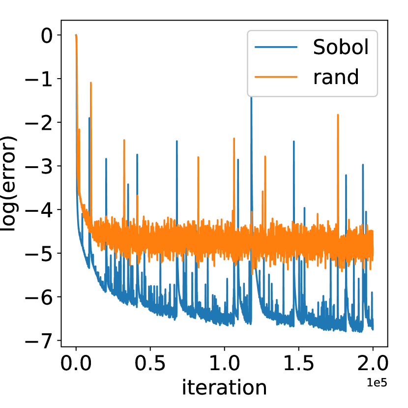
Relative errors in different dimensions and the corresponding convergence rates with respect to the mini-batch size are shown in Table 2 and Table 3, respectively. Since there are some oscillations as the iteration increases, each point here represents the error averaged over iterations. The total number of iterations is set to be . It is reasonable to find that QMC method performs better than MC method as shown in Tables 2 and 3. When the size of mini-batches increases, the advantage of QMC method over MC method reduces. This is natural in the sense that both methods converges when the number of sampling points increases. We further plot detained training processes of QMC and MC methods in Figure 3. Clearly, QMC sampling reduces the magnitude of error of MC method by about three times on average with the same mini-batch size for the 2D problem.
| Dimension | mini-batch size | QMC | MC | ||
|---|---|---|---|---|---|
| error() | order | error() | order | ||
| 2D | 500 | 1.7141 | 4.2706 | ||
| 1000 | 1.1420 | 0.59 | 3.4157 | 0.32 | |
| 2000 | 0.7702 | 0.59 | 2.6225 | 0.38 | |
| 4000 | 0.6401 | 0.27 | 2.2505 | 0.22 | |
| 4D | 500 | 1.8735 | 3.5183 | ||
| 1000 | 1.4468 | 0.37 | 3.0786 | 0.19 | |
| 2000 | 1.0557 | 0.45 | 2.6561 | 0.21 | |
| 4000 | 0.8076 | 0.39 | 2.0410 | 0.38 | |
| 8D | 500 | 2.0737 | 2.4514 | ||
| 1000 | 1.5714 | 0.40 | 2.2083 | 0.15 | |
| 2000 | 1.1607 | 0.43 | 2.0297 | 0.12 | |
| 10000 | 0.8139 | 0.22 | 1.1551 | 0.35 | |
| 16D | 2000 | 0.8613 | 2.0754 | ||
| 5000 | 0.6863 | 0.25 | 1.3506 | 0.47 | |
| 10000 | 0.5361 | 0.36 | 1.1383 | 0.25 | |
| 20000 | 0.4623 | 0.21 | 1.2298 | 0.11 | |
| Dimension | QMC | MC |
|---|---|---|
| 2D | 0.48 | 0.32 |
| 4D | 0.41 | 0.26 |
| 8D | 0.31 | 0.26 |
| 16D | 0.28 | 0.24 |
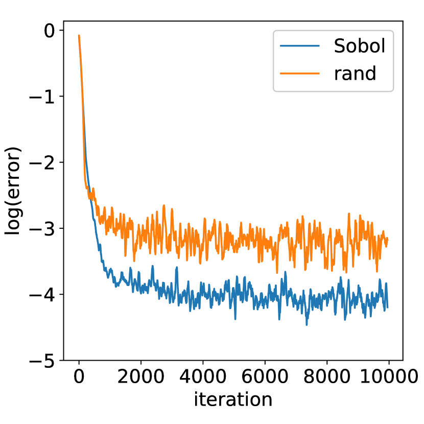
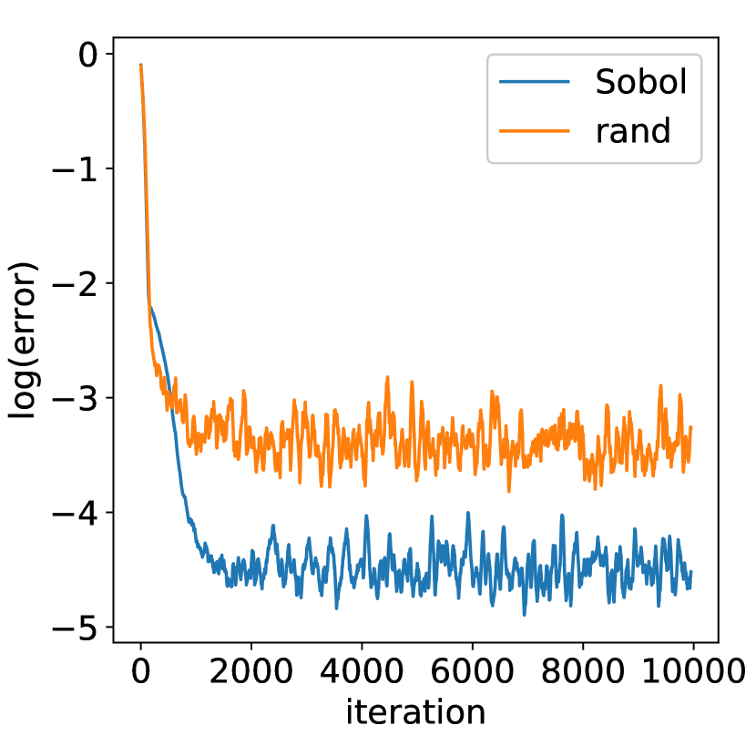
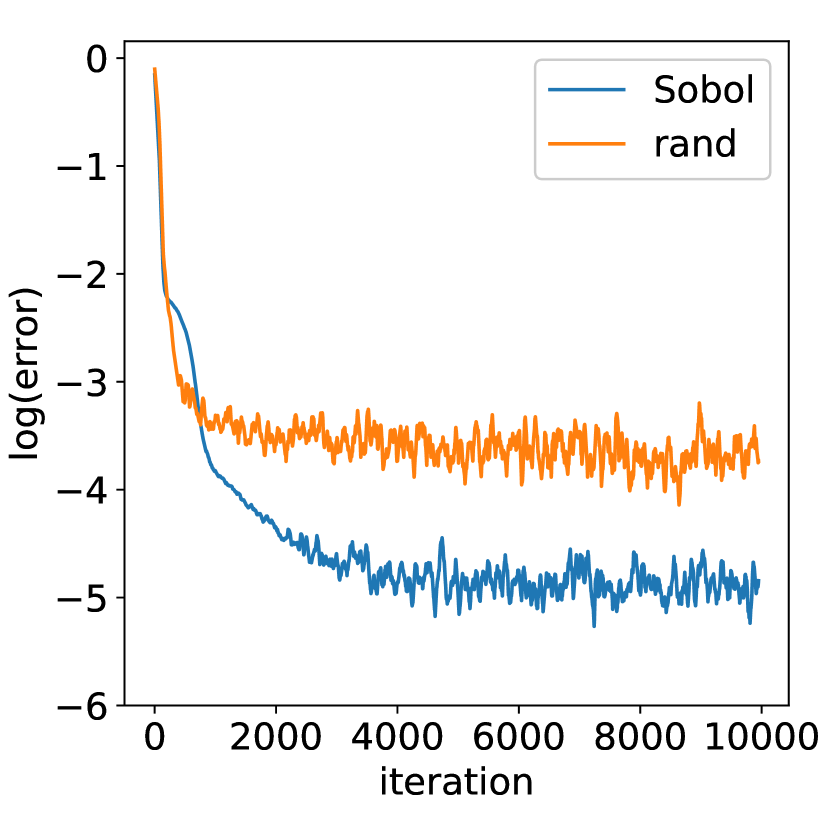
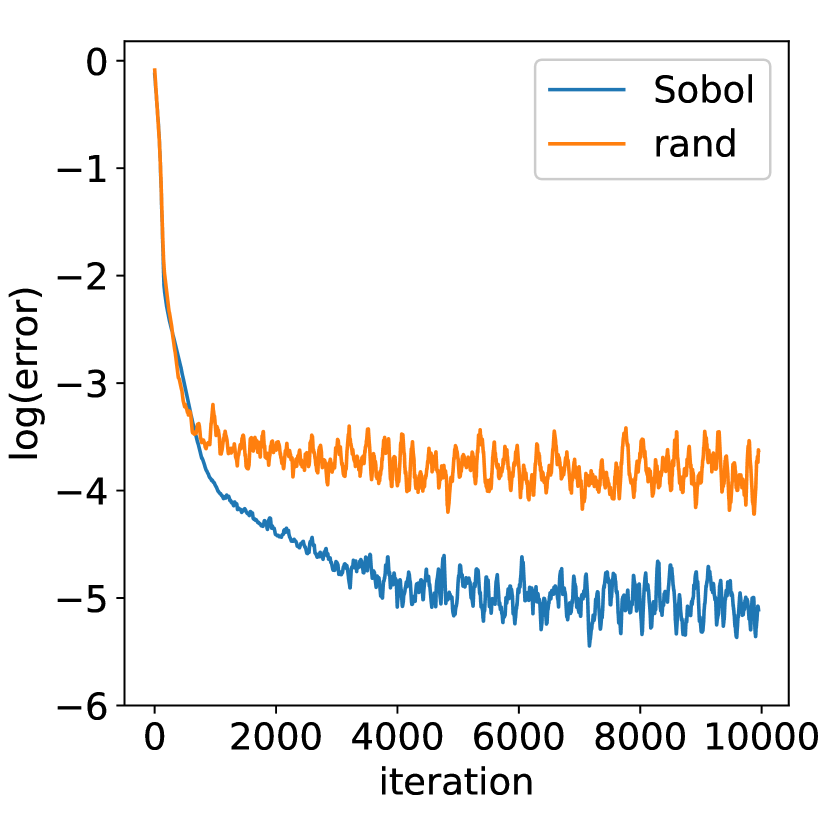
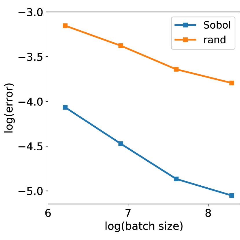
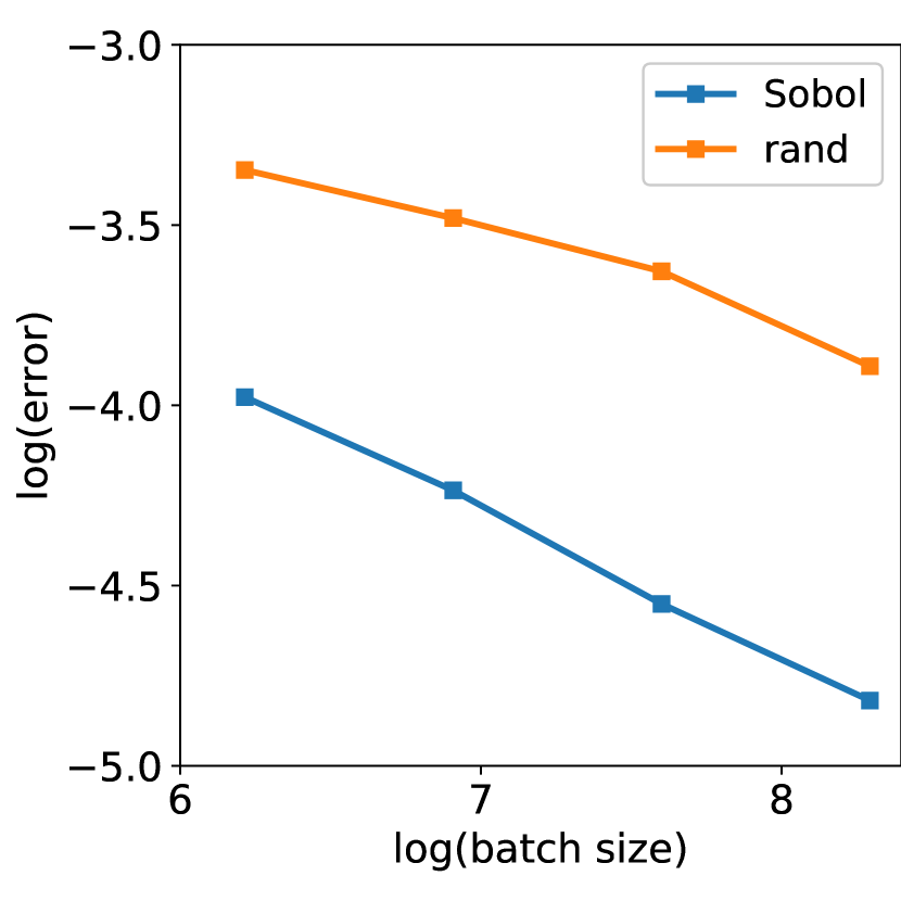
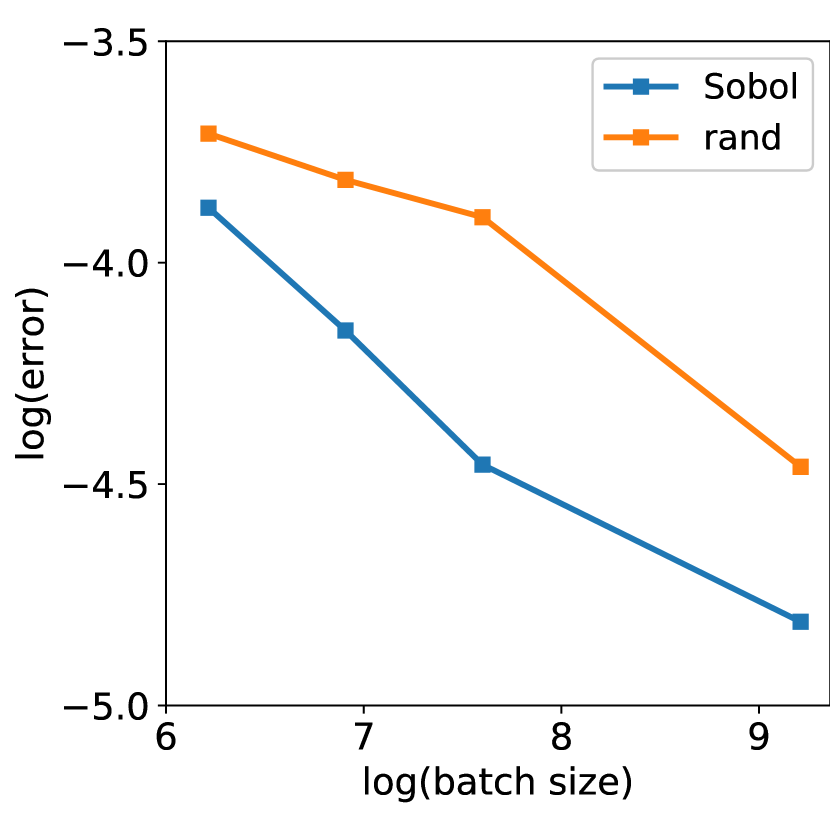
Figure 4 plots relative error in terms of mini-batch size for QMC and MC methods for (17) from 2D to 16D. A clear evidence is that QMC method always outperforms MC method and the error reduction is significant.
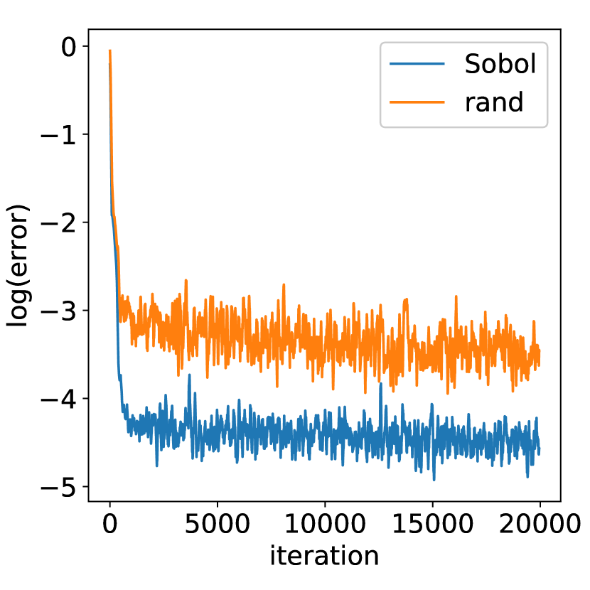
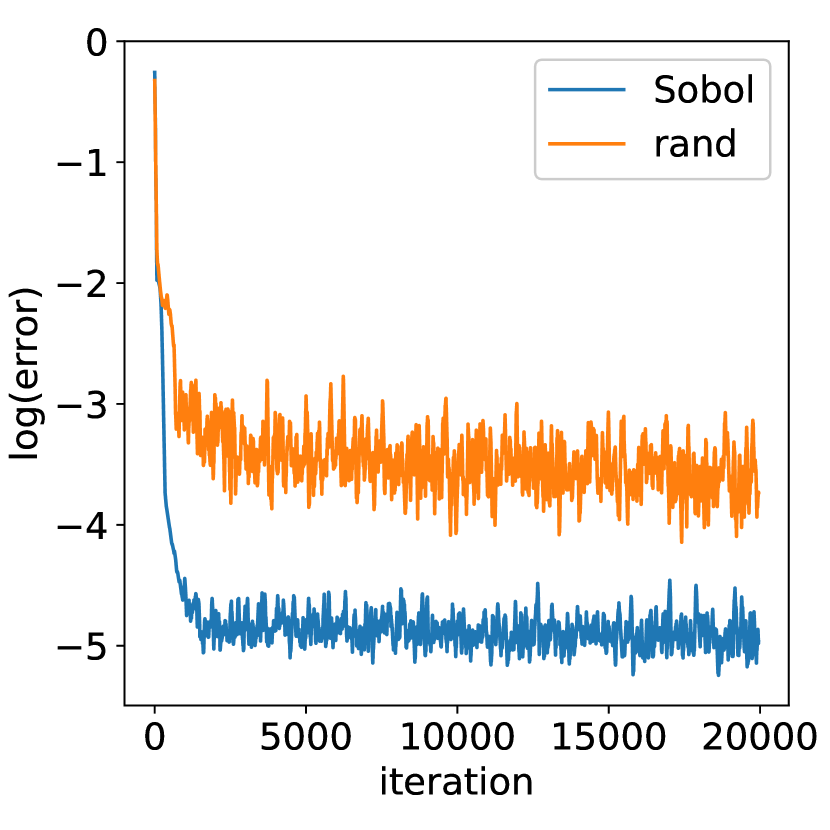
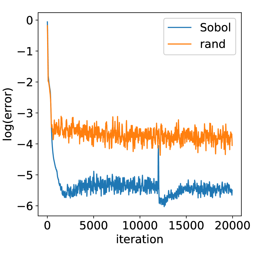
From a different perspective, in order to achieve the same approximation accuracy, we may ask how much cheaper QMC method is compared to MC method. To do this, we fix the mini-batch size in MC method to be and , and check the corresponding size in QMC method for the same accuracy requirement. Results are recorded in Table 4, and detailed training processes in 2D are plotted in Figure 5. For the same accuracy requirement, compared to MC method, QMC method reduces the size of training data set by more than two orders of magnitude.
| Dimension | MC | QMC | ||
|---|---|---|---|---|
| size | error() | size | error() | |
| 2D | 10000 | 1.3566 | 500 | 1.7141 |
| 100000 | 0.7702 | 2000 | 0.6149 | |
| 4D | 10000 | 1.8462 | 500 | 1.8735 |
| 100000 | 0.8986 | 4000 | 0.8076 | |
| 8D | 10000 | 1.1551 | 2000 | 1.1607 |
| 100000 | 0.8668 | 10000 | 0.8139 | |
| 16D | 10000 | 1.1383 | 1000 | 1.0472 |
| 100000 | 0.7993 | 5000 | 0.6863 | |
All above results show that QMC method always performs better than MC method, typically by several times in terms of accuracy when the same mini-batch size is enforced or by more than two orders of magnitude in terms of efficiency when the same accuracy is required. However, their convergence rates with respect to both the iteration number and the size of training data set seem to be the same, due to the ADAM optimizer we used and the nonconvex nature of loss function.
3.2 Neumann problem
Consider a Neumann problem over
| (19) |
with the exact solution and being the unit outward normal vector. For this problem, we still do not need to add any penalty term for the boundary condition and the loss function is defined as
| (20) |
The network structure is the same as before; see (8). Detailed setup is listed in Table 5. Exact and trained solutions in 2D are visualized in Figure 6. Relative errors in differential dimensions are recorded in Table 6 and the corresponding convergence rates are shown in Table 7.
| Dimension | Blocks | Parameters | |
|---|---|---|---|
| 2 | 4 | 10 | 921 |
| 4 | 4 | 15 | 2011 |
| 8 | 4 | 30 | 7741 |
| 16 | 5 | 48 | 24385 |
| Dimension | mini-batch size | QMC | MC | ||
|---|---|---|---|---|---|
| error() | order | error() | order | ||
| 2D | 250 | 1.1218 | 2.9571 | ||
| 500 | 0.7484 | 0.58 | 2.6754 | 0.14 | |
| 1000 | 0.4314 | 0.79 | 2.2572 | 0.25 | |
| 2000 | 0.3140 | 0.46 | 1.9914 | 0.18 | |
| 4D | 500 | 1.4219 | 3.9305 | ||
| 1000 | 0.9185 | 0.63 | 3.6990 | 0.09 | |
| 2000 | 0.3289 | 1.48 | 2.4779 | 0.58 | |
| 4000 | 0.2649 | 0.24 | 2.0152 | 0.23 | |
| 8D | 500 | 3.8542 | 7.7874 | ||
| 1000 | 2.7353 | 0.49 | 6.2379 | 0.32 | |
| 2000 | 2.4249 | 0.17 | 5.4659 | 0.19 | |
| 10000 | 1.8235 | 0.18 | 2.6860 | 0.44 | |
| 16D | 1000 | 3.2668 | 6.0573 | ||
| 2000 | 2.9308 | 0.16 | 5.8566 | 0.05 | |
| 5000 | 2.9205 | 0.01 | 4.8035 | 0.22 | |
| 10000 | 1.5636 | 0.90 | 3.8518 | 0.32 | |
| Dimension | QMC | MC |
|---|---|---|
| 2D | 0.63 | 0.20 |
| 4D | 0.78 | 0.32 |
| 8D | 0.23 | 0.35 |
| 16D | 0.28 | 0.20 |
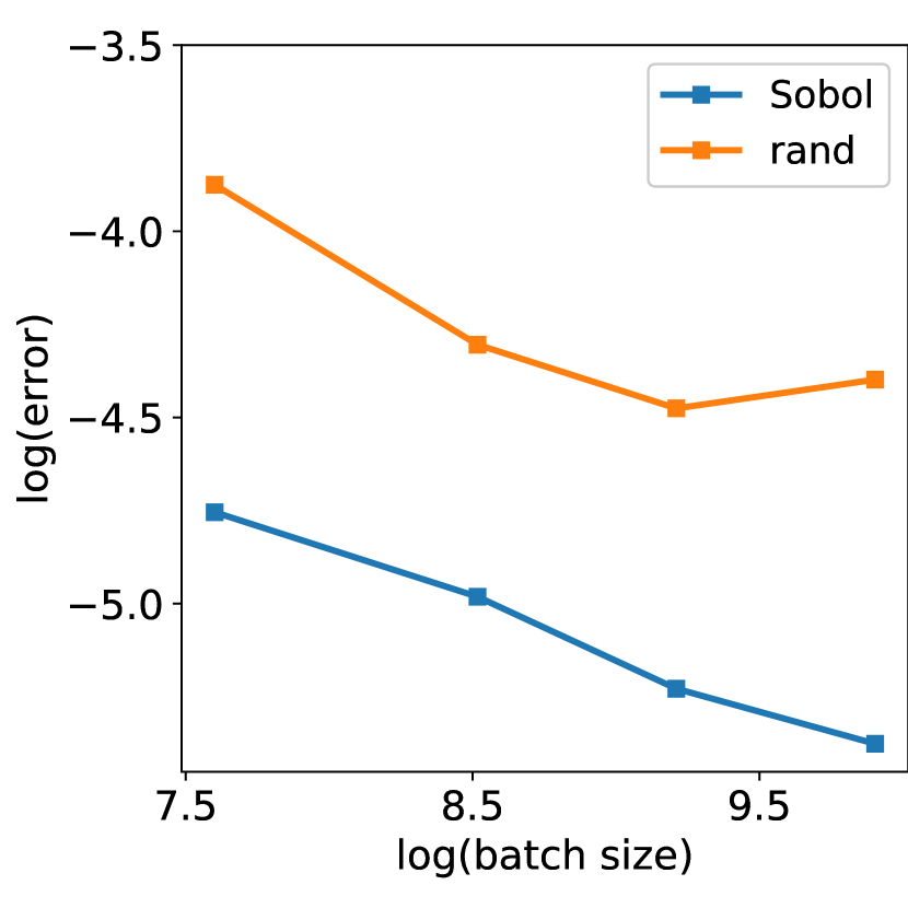
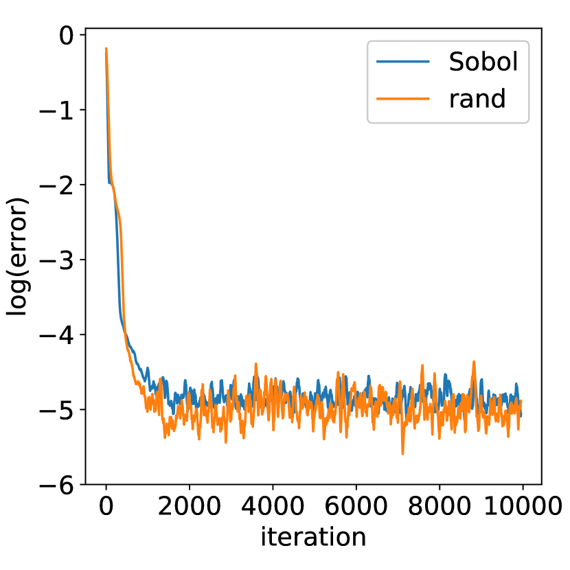
Figure 6 plots detailed training processes of QMC and MC methods for different mini-batch sizes in 2D. Similarly, QMC method outperforms MC method by several times in terms of accuracy for the same size of training data set.
Besides, for the same accuracy requirement, QMC reduces the size of training data set by orders of magnitudes; see Table 8 as well as Figure 8 for details.
| Dimension | MC | QMC | ||
|---|---|---|---|---|
| size | error() | size | error() | |
| 2D | 10000 | 1.3138 | 250 | 1.1218 |
| 100000 | 0.6536 | 500 | 0.7484 | |
| 4D | 10000 | 2.0778 | 500 | 1.4218 |
| 100000 | 0.4622 | 2000 | 0.3289 | |
| 8D | 10000 | 2.6860 | 1000 | 2.7353 |
| 100000 | 2.5154 | 2000 | 2.4249 | |
| 16D | 10000 | 3.8518 | 1000 | 3.2668 |
| 100000 | 2.7805 | 5000 | 2.9205 | |
Generally speaking, not every Neumann problem can be modeled by a loss function without the penalty term on the boundary. Therefore, for a general Neumann problem of the form
| (21) |
we add the penalty term into the loss function (20)
| (22) |
The first term is a volume integral while the second term is a boundary integral. Therefore, we have to sample these two terms separately: one for in and the other for the penalty term on the boundary. In principle, we need to optimize sizes of both training sets in order to minimize the approximation error. Practically, we find that QMC method always performs better than MC method. In Table 9, we show relative errors in different dimensions with different mini-batch sizes for Neumann problem with the penalty term on the boundary.
| Dimension | Mini-batch size | Relative error | ||
|---|---|---|---|---|
| Volume | Boundary | QMC() | MC() | |
| 2D | 250 | 100 | 0.8079 | 1.6151 |
| 500 | 100 | 0.4176 | 1.5027 | |
| 1000 | 100 | 0.2086 | 1.0101 | |
| 2000 | 100 | 0.1470 | 0.8327 | |
| 4D | 500 | 100 | 0.4434 | 1.7622 |
| 1000 | 100 | 0.3729 | 1.2550 | |
| 2000 | 100 | 0.3160 | 0.9799 | |
| 4000 | 100 | 0.2651 | 0.7530 | |
| 8D | 500 | 100 | 1.1770 | 3.8285 |
| 1000 | 100 | 0.8989 | 3.0505 | |
| 2000 | 100 | 0.8780 | 2.9661 | |
| 10000 | 100 | 0.7643 | 1.6552 | |
| 16D | 1000 | 100 | 1.2181 | 3.1398 |
| 2000 | 100 | 1.1250 | 2.2055 | |
| 5000 | 100 | 0.8998 | 1.9235 | |
| 10000 | 100 | 0.7698 | 1.5244 | |
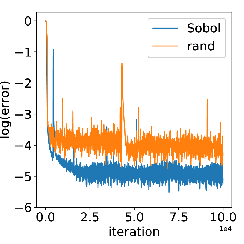
Figure 9 plots detailed training processes of QMC and MC methods for different mini-batch sizes for Neumann problem with the penalty term on the boundary in 2D. Size of the training data set for the penalty term is fixed to be in all cases.
4 Convergence analysis
To understand numerical results in §3 from a theoretical perspective, in this section, we shall analyze the convergence behavior of SGD method with QMC sampling and understand how the size of training data set affects the convergence for different sampling strategies. Our analysis follows [21], but differs in terms of assumptions. Under the boundedness assumption of parameter sequence, we prove the Lipschitz continuity of loss function for smooth activation functions, such as (6), instead of the direct assumption of Lipschitz continuity of loss function. From a practical perspective, our assumption can be easily verified during the iteration while the Lipschitz continuity is difficult to be verified. Moreover, we prove the convergence of function sequences generated by MC and QMC methods under a stronger assumption on the second moment of the stochastic vector used in the SGD method, which explicitly characterizes the dependence of convergence rate on both the size of training data set and the iteration number.
For convenience, derivatives are taken with respect to the parameter set if subscripts are not specified in what follows. We start with the following assumption.
Assumption 4.1 (Boundedness of the iteration sequence).
The iteration sequence is bounded, i.e., ,
A direct consequence of Assumption 4.1 is the existence of convergent sub-sequences. It will be shown later that the whole sequence of function values generated by the SGD method with a sampling strategy converges if the loss function is strongly convex with respect to . In practice, this assumption can be verified easily in the iteration. Furthermore, we choose a activation function ; see (6). Consequently, the residual network also belongs to with respect to both and . Therefore, the Lipschitz continuity of the approximate solution by the neural network is guaranteed in a bounded domain.
Lemma 4.2.
Under Assumption 4.1, the activation function, and the bounded domain , there exist constants , and , and such that
A natural corollary of Lemma 4.2 is that there exist constants and , and , such that
| (23) |
Remember that above results hold for smooth activation functions, but does not hold for ReLU activation function. Then we can only expect the boundness of and , instead of Lipschitz continuity. For example, consider the simplest network with two layers. For the ReLU activation function [37], there exists a constant depending on such that
| (24) |
Based on Lipschitz continuity of the neural network solution and boundedness of derivatives, Lipschitz continuity of the loss function can be proven.
Theorem 4.3 (Lipschitz continuity of the loss function).
For any and , the loss function of the neural network satisfies
| (25) |
Proof.
An important consequence of the Theorem 4.3 is that for ,
| (26) |
To proceed, we need the following assumptions.
Assumption 4.4 (First and second moment assumption).
For the stochastic vector, assume that first and second moments satisfy
-
•
There exists such that, ,
(27) and
(28) -
•
For the second moment, there exist and such that, ,
(29)
where , and for MC sampling and for QMC sampling.
Note that is an unbiased estimate of as when in Assumption 4.4. Moreover, according to (29), we have
with . For a fixed stepsize , according to (26), we have
| (30) |
Assumption 4.5 (Strong convexity).
The loss function is strongly convex with respect to , i.e., there exists a constant , , such that
Theorem 4.6 (Strongly convex loss function, fixed stepsize, MC and QMC samplings).
Proof.
Theorem 4.6 provides a quantitative estimate of the accuracy of sampling strategies on the convergence rate of the iteration sequence. Regardless of the sampling strategy, the convergence rate is linear which is determined by the SGD method.
Remark 4.1.
When , for both MC and QMC methods, we have . Form Theorem 4.6, we conclude that
In practice, however, with the increasing size of training data set, the gap usually does not tend to under the fixed stepsize condition. We attributes this to the irrationality of (29). Instead, (29) shall be relaxed to [21]
Then we have
which implies the convergence of the sequence of function values near the optimal value. Therefore, an optimizer with fixed stepsize is generally not the best choice [21]. Instead, the SGD method with diminishing stepsize is popular in real applications, such as ADAM method [36] using in the implementation.
Remark 4.2.
From the convergence analysis (32), we expect that QMC method outperforms MC method in terms of convergence order. It is reasonable to find from Tables 3 and 7 that QMC method has better rates than MC method. However, the difference in rate is not as significant as the difference in magnitude. We attribute this difference to the nonconvexity of the loss function and the above analysis relies crucially on the strong convexity assumption of the same function. Whatever, for the same accuracy requirement in practice, QMC method outperforms MC method in terms of efficiency by orders of magnitude. Therefore, we recommend the usage of QMC sampling in machine-learning PDEs whenever a sampling strategy is needed.
5 Conclusion
In this paper, we have proposed to approximate the loss function using quasi-Monte Carlo method, instead of Monte Carlo method that is commonly used in machine-learning PDEs. Numerical results based on deep Ritz method have shown the significant advantage of quasi-Monte Carlo method in terms of accuracy or efficiency. All the codes that generate numerical results included in this work are available from https://github.com/Lyupinpin/DeepRitzMethod.
Theoretically, we have proved the convergence of neural network solver based on quasi-Monte Carlo sampling in terms of the sampling size and the iteration number. Although there are practical issues such as the nonconvexity of the loss function, our analysis does provide a comprehensive understanding of why quasi-Monte Carlo method always outperforms Monte-Carlo method and suggests the usage of the former whenever an approximation of high-dimensional integrals is needed.
Acknowledgements
This work is supported in part by the grants NSFC 21602149 and 11971021 (J. Chen), NSFC 11501399 (R. Du). P. Li is grateful to Ditian Zhang for very helpful discussions. L. Lyu acknowledges the financial support of Undergraduate Training Program for Innovation and Entrepreneurship, Soochow University (Projection 201810285019Z). Part of the work was done when L. Lyu was doing a summer internship at Department of Mathematics, Hong Kong University of Science and Technology. L. Lyu would like to thank its hospitality.
References
- [1] Weinan E and Bing Yu. The deep ritz method: A deep learning-based numerical algorithm for solving variational problems. Communications in Mathematics and Statistics, 6(1):1–12, 2018.
- [2] Ian Goodfellow, Yoshua Bengio, and Aaron Courville. Deep Learning. MIT Press, 2016.
- [3] Tao Wang, David J. Wu, Adam Coates, and Andrew Y. Ng. End-to-end text recognition with convolutional neural networks. Proceedings of the 21st International Conference on Pattern Recognition (ICPR2012), pages 3304–3308, 2012.
- [4] Alex Krizhevsky, Ilya Sutskever, and Geoffrey E. Hinton. Imagenet classification with deep convolutional neural networks. Communications of the ACM, 60:84–90, 2012.
- [5] Hinton Geoffrey, Deng Li, Yu Dong, Dahl George, Mohamed Abdel-rahman, Jaitly Navdeep, Senior Andrew, Vanhoucke Vincent, Nguyen Patrick, Kingsbury Brian, and Sainath Tara. Deep neural networks for acoustic modeling in speech recognition. IEEE Signal Processing Magazine, 29:82–97, 2012.
- [6] Ruhi Sarikaya, Geoffrey E. Hinton, and Anoop Deoras. Application of deep belief networks for natural language understanding. IEEE/ACM Transactions on Audio, Speech, and Language Processing, 22(4):778–784, 2014.
- [7] Jiequn Han, Arnulf Jentzen, and Weinan E. Solving high-dimensional partial differential equations using deep learning. PNAS, 115(34):8505–8510, 2018.
- [8] Yuwei Fan, Feliu-Fabà Jordi, Lin Lin, Lexing Ying, and Leonardo Zepeda-Núñez. A multiscale neural network based on hierarchical nested bases. Research in the Mathematical Sciences, 6(2):21, 2019.
- [9] Justin Sirignano and Konstantinos Spiliopoulos. DGM: A deep learning algorithm for solving partial differential equations. Journal of Computational Physics, 375:1339–1364, 2018.
- [10] Carleo Giuseppe and Troyer Matthias. Solving the quantum many-body problem with artificial neural networks. Science, 355(6325):602–606, 2017.
- [11] Jiequn Han, Linfeng Zhang, and Weinan E. Solving many-electron schrödinger equation using deep neural networks. Journal of Computational Physics, 399, 2019.
- [12] Weinan E, Jiequn Han, and Arnulf Jentzen. Deep learning-based numerical methods for high-dimensional parabolic partial differential equations and backward stochastic differential equations. Communications in Mathematics and Statistics, 5(4):349–380, 2017.
- [13] Christian Beck, Weinan E, and Arnulf Jentzen. Machine learning approximation algorithms for high-dimensional fully nonlinear partial differential equations and second-order backward stochastic differential equations. Journal of Nonlinear Science, 29(4):1563–1619, 2019.
- [14] J A González Cervera. Solution of the black-scholes equation using artificial neural networks. Journal of Physics: Conference Series, 1221:012044, 2019.
- [15] Randall J. LeVeque. Finite Difference Methods for Ordinary and Partial Differential Equations: Steady-State and Time-Dependent Problems. Society for Industrial and Applied Mathematics, 2007.
- [16] Susanne C. Brenner and L. Ridgway Scoot. The Mathematical Theory of Finite Element Method. Springer, 2007.
- [17] Jie Shen, Tao Tang, and Li-Lian Wang. Spectral methods: Algorithm, Analysis and Application. Springer, 2011.
- [18] Thomas Gerstner and Michael Griebel. Numerical integration using sparse grids. Numerical Algorithms, 18(3-4):209, January 1998.
- [19] Hans-Joachim Bungartz and Michael Griebel. Sparse grids. Acta Numerica, 13:147–269, May 2004.
- [20] Xiaobing Feng, Thomas Lewis, and Michael Neilan. Discontinuous Galerkin finite element differential calculus and applications to numerical solutions of linear and nonlinear partial differential equations. Journal of Computational and Applied Mathematics, 299:68–91, 2016.
- [21] Léon Bottou, Frank E. Curtis, and Jorge Nocedal. Optimization for large-scale machine learning. SIAM Review, 60(2):223–311, 2018.
- [22] Jun S Liu. Monte Carlo strategies in scientific computing. Springer Science & Business Media, 2008.
- [23] Yosihiko Ogata. A Monte Carlo method for high dimensional integration. Numerische Mathematik, 55(2):137–157, 1989.
- [24] H. Niederreiter. Random number generation and quasi-Monte Cralo methods. CBMS-SIAM, 63, 1992.
- [25] Josef Dick, Frances Y. Kuo, and Ian H. Sloan. High-dimensional integration: The quasi-Monte Carlo way. Acta Numerical, 22:133–288, 2013.
- [26] Bruno Tuffin. Randomization of Quasi-Monte Carlo methods for error estimation: survey and normal approximation. Monte Carlo Methods and Applications, 10(3):617–628, 2004.
- [27] Alexander Buchholz, Florian Wenzel, and Stephan Mandt. Quasi-Monte Carlo variational inference. arXiv, 1807.01604, 2018.
- [28] Liyao Lyu, Zhiwen Zhang, and Jingrun Chen. Connecting exciton diffusion with surface roughness via deep learning. arXiv, 1910.14209, 2019.
- [29] Evans C. Lawrence. Partial differential equations(second edition). American Mathematical Society, 2010.
- [30] Prajit Ramachandran, Barret Zoph, and Quoc V. Le. Searching for activation functions. arXiv, 1710.05941, 2017.
- [31] Kaiming He, Xiangyu Zhang, Shaoqing Ren, and Jian Sun. Deep residual learning for image recognition. 2016 IEEE Conference on Computer Vision and Pattern Recognition (CVPR), 2:770–778, 2016.
- [32] Harald Niederreiter. Random number generation and quasi-Monte Carlo methods. SIAM, 1992.
- [33] Russel Caflisch. Monte Carlo and quasi-Monte Carlo methods, volume 7. Cambridge University Press.
- [34] Josef Dick, Frances Y. Kuo, and Ian H. Sloan. High-dimensional integration: the quasi-Monte Carlo way. Acta Numerica, 22:133–288, 2013.
- [35] I. M. Sobol. Uniformly distributed sequences with an additional uniform property. USSR Computational Mathematics and Mathematical Physics, 16(5):236–242, 1976.
- [36] Diederik P. Kingma and Jimmy Ba. Adam: A method for stochastic optimization. CoRR, 1412.6980, 2014.
- [37] Vinod Nair and Geoffrey E Hinton. Rectified linear units improve restricted boltzmann machines. In Proceedings of the 27th international conference on machine learning (ICML-10), pages 807–814, 2010.