AReN: Assured ReLU NN Architecture for Model Predictive Control of LTI Systems

Abstract.

In this paper, we consider the problem of automatically designing a Rectified Linear Unit (ReLU) Neural Network (NN) architecture that is sufficient to implement the optimal Model Predictive Control (MPC) strategy for an LTI system with quadratic cost. Specifically, we propose AReN, an algorithm to generate Assured ReLU Architectures. AReN takes as input an LTI system with quadratic cost specification, and outputs a ReLU NN architecture with the assurance that there exist network weights that exactly implement the associated MPC controller. AReN thus offers new insight into the design of ReLU NN architectures for the control of LTI systems: instead of training a heuristically chosen NN architecture on data – or iterating over many architectures until a suitable one is found – AReN can suggest an adequate NN architecture before training begins. While several previous works were inspired by the fact that both ReLU NN controllers and optimal MPC controller are both Continuous, Piecewise-Linear (CPWL) functions, exploiting this similarity to design NN architectures with correctness guarantees has remained elusive. AReN achieves this using two novel features. First, we reinterpret a recent result about the implementation of CPWL functions via ReLU NNs to show that a CPWL function may be implemented by a ReLU architecture that is determined by the number of distinct affine regions in the function. Second, we show that we can efficiently over-approximate the number of affine regions in the optimal MPC controller without solving the MPC problem exactly. Together, these results connect the MPC problem to a ReLU NN implementation without explicitly solving the MPC and directly translates this feature to a ReLU NN architecture that comes with the assurance that it can implement the MPC controller. We show through numerical results the effectiveness of AReN in designing an NN architecture.

1. Introduction

End-to-end learning is attractive for the realization of autonomous cyber-physical systems, thanks to the appeal of control systems based on a pure data-driven architecture. By taking advantage of the current advances in the field of reinforcement learning, several works in the literature showed how a well trained deep NN that is capable of controlling cyber-physical systems to achieve certain tasks (bojarski2016end, ). Nevertheless, the current state-of-the-art practices of designing these deep NN-based controllers is based on heuristics and hand-picked hyper-parameters (e.g., number of layers, number of neurons per layer, training parameters, training algorithm) without an underlying theory that guides their design. In this paper, we focus on the fundamental question of how to systematically choose the NN architecture (number of layers and number of neurons per layer) such that we guarantee the correctness of the chosen NN architecture.

In this paper, we will confine our attention to the state-feedback Model Predictive Control (MPC) of a Linear Time-Invariant (LTI) system with quadratic cost and under input and output constraints (see Section 2 for the specific MPC formulation). Importantly, this MPC control problem is known to have a solution that is Continuous and Piecewise-Linear (CPWL) in the current system state (BemporadExplicitLinearQuadratic2002, ). This property renders optimal MPC controllers compatible with a ReLU NN implementation, as any ReLU NN defines a CPWL function of its inputs. For this reason, several recent papers focus on how to approximate an optimal MPC controller using a ReLU NN (ChenApproximatingExplicitModel2018, ).

However, unlike other work on the subject, AReN seeks to use knowledge of the underlying control problem to guide the design of data-trained NN controllers. One of the outstanding problems with data-driven approaches is that the architecture for the NN is chosen either according to heuristics or else via a computationally expensive iteration scheme that involves adapting the architecture iteratively and re-training the NN. Besides being computationally taxing, neither of these provide any assurances that the resultant architecture is sufficient to adequately control the underlying system, either in terms of performance or stability. In the context of controlling an LTI system, then, AReN partially addresses these shortcomings: AReN is a computationally pragmatic algorithm that returns a ReLU NN architecture that is at least sufficient to implement the optimal MPC controller described before. That is given an LTI system with quadratic cost and input/output constraints, AReN determines a ReLU NN architecture – both its structure and its size – with the guarantee that there exists an assignment of the weights such that the resultant NN exactly implements the optimal MPC controller. This architecture can then be trained on data to obtain the final controller, only now with the assurance that the training algorithm can choose the optimal MPC controller among all of the possible NN weight assignments available to it.

The algorithm we propose depends on two observations:

• First, that any CPWL function may be translated into a ReLU NN with an architecture determined wholly by the number of linear regions in the function; this comes from a careful interpretation of the recent results in (AroraUnderstandingDeepNeural2016, ), which are in turn based on the hinging-hyperplane characterization of CPWL functions in (ShuningWangGeneralizationHingingHyperplanes2005, ) and the lattice characterization of CPWL functions in (KahlertGeneralizedCanonicalPiecewiselinear1990, ).

• Second, that there is a computationally efficient way to over-approximate the number of linear regions in the optimal MPC controller without solving for the optimal controller explicitly. This involves converting the state-region specification equation for the optimal controller into a single, state-independent collection of linear-inequality feasibility problems – at the expense of over-counting the number of affine regions that might be present in the optimal MPC controller. This requires an algorithmic solution rather than a closed form one, but the resultant algorithm is computationally efficient enough to treat much larger problems than are possible when the explicit optimal controller is sought.

Together these observations almost completely specify an algorithm that provides the architectural guidance we claim.

Related work: The idea of training neural networks to mimic the behavior of model predictive controllers can be traced back to the late 1990s where neural networks trained to imitate MPC controllers were used to navigate autonomous robots in the presence of obstacles (see for example (ortega1996mobile, ), and the references within) and to stabilize highly nonlinear systems (cavagnari1999neural, ). With the recent advances in both the fields of NN and MPC, several recent works have explored the idea of imitating the behavior of MPC controllers  (hertneck2018learning, ; aakesson2006neural, ; pereira2018mpc, ; amos2018differentiable, ; claviere2019trajectory, ). The focus of all this work was to blindly mimic a base MPC controller without exploiting the internal structure of the MPC controller to design the NN structure systematically. The closest to our work are the results reported in (karg2018efficient, ; ChenApproximatingExplicitModel2018, ). In this line of work, the authors were motivated by the fact that both explicit state MPC and ReLU NNs are CPWL functions, and they studied how to compare the performance of trained NN and explicit state MPC controllers. Different than the results reported in  (karg2018efficient, ; ChenApproximatingExplicitModel2018, ), we focus, in this paper, on how to bridge the insights of explicit MPC to provide a systematic way to design a ReLU NN architecture with correctness guarantees.

Another related line of work is the problem of Automatic Machine Learning (AutoML) and in particular the problem of hyperparameter (number of layers, number of neurons per layer, and learning algorithm parameters) optimization and tuning in deep NN, in general, and in deep reinforcement learning, in particular (see for example (pedregosa2016hyperparameter, ; bergstra2012random, ; paul2019fast, ; baker2016designing, ; quanming2018taking, ) and the references within). In this line of work, an iterative and exhaustive search through a manually specified subset of the hyperparameter space is performed. Such a search procedure is typically followed by the evaluation of some performance metric that is used to select the best hyperparameters. Unlike the results reported in this line of work, AReN does not iterate over several designs to choose one. Instead, AReN directly generates an NN architecture that is guaranteed to control the underlying physical system adequately.

2. Problem Formulation

2.1. Dynamical Model and Neural Network Controller

We consider a discrete-time Linear, Time-Invariant (LTI) dynamical system of the form:

(1) $$x(t+1) =Ax(t)+Bu(t),\qquad y(t)=Cx(t)$$

where $x(t)\in\mathbb{R}^{n}$ is the state vector at time $t\in\mathbb{N}$, $u(t)\in\mathbb{R}^{m}$ is the control vector, and $y(t)\in\mathbb{R}^{l}$ is the output vector. The matrices $A$, $B$, and $C$ represents the system dynamics and the output map and have appropriate dimensions. Furthermore, we consider controlling (1) with a state feedback neural network controller ${\mathscr{N}\negthickspace\negthickspace\negthinspace\mathscr{N}}\negthinspace$:

(2) $${\mathscr{N}\negthickspace\negthickspace\negthinspace\mathscr{N}}\negthinspace:\mathbb{R}^{n}\rightarrow\mathbb{R}^{m}$$

while fulfilling the constraints:

(3) $$y_{\text{min}}\leq y(t)\leq y_{\text{max}},\qquad u_{\text{min}}\leq u(t)\leq u_{\text{max}}$$

at all time instances $t\geq 0$ where $y_{\text{min}},y_{\text{max}},u_{\text{min}}$ and $u_{\text{max}}$ are constant vectors of appropriate dimension with $y_{\text{min}}<y_{\text{max}}$ and $u_{\text{min}}<u_{\text{max}}$ (where $<$ is taken element-wise).

In particular, we consider a ($K$-layer) Rectified Linear Unit Neural Network (ReLU NN) that is specified by composing $K$ layer functions (or just layers). A layer with $\mathfrak{i}$ inputs and $\mathfrak{o}$ outputs is specified by a $(\mathfrak{o}\times\mathfrak{i})$ real-valued matrix of weights, $W$, and a $(\mathfrak{o}\times 1)$ real-valued matrix of biases, $b$, as follows:

$$L_{\theta}:\mathbb{R}^{\mathfrak{i}} \rightarrow\mathbb{R}^{\mathfrak{o}}$$

(4) $$z \mapsto\max\{Wz+b,0\}$$

where the $\max$ function is taken element-wise, and $\theta\triangleq(W,b)$ for brevity. Thus, a $K$-layer ReLU NN function as above is specified by $K$ layer functions $\{L_{\theta^{(i)}}:i=1,\dots,K\}$ whose input and output dimensions are composable: that is they satisfy $\mathfrak{i}_{i}=\mathfrak{o}_{i-1}:i=2,\dots,K$. Specifically:

(5) $${\mathscr{N}\negthickspace\negthickspace\negthinspace\mathscr{N}}\negthinspace(x)=(L_{\theta^{(K)}}\circ L_{\theta^{(K-1)}}\circ\dots\circ L_{\theta^{(1)}})(x).$$

When we wish to make the dependence on parameters explicit, we will index a ReLU function ${\mathscr{N}\negthickspace\negthickspace\negthinspace\mathscr{N}}\negthinspace$ by a list of matrices $\Theta\triangleq(\theta^{(1)},\dots,\theta^{(K)})$ . Also, it is common to allow the final layer function to omit the $\max$ function altogether, and we will be explicit about this when it is the case.

Note that specifying the number of layers and the dimensions of the associated matrices $\theta^{(i)}=(\;W^{(i)},b^{(i)}\;)$ specifies the architecture of the ReLU NN. Therefore, we will use:

(6) $$\text{Arch}(\Theta)\triangleq((n,\mathfrak{o}_{1}),(\mathfrak{i}_{2},\mathfrak{o}_{2}),\ldots,(\mathfrak{i}_{K-1},\mathfrak{o}_{K-1}),(\mathfrak{i}_{K},m))$$

to denote the architecture of the ReLU NN ${\mathscr{N}\negthickspace\negthickspace\negthinspace\mathscr{N}}\negthinspace_{\Theta}$. Note that our definition is general enough since it allows the layers to be of different sizes, as long as $\mathfrak{o}_{i-1}=\mathfrak{i}_{i}$ for $i=2,\dots,K$.

2.2. Neural Network Architecture Specification

We are interested in finding an architecture $\text{Arch}(\Theta)$ for the ${\mathscr{N}\negthickspace\negthickspace\negthinspace\mathscr{N}}\negthinspace_{\Theta}$ such that it is guaranteed to have enough parameters to exactly mimic the input-output behavior of some base controller $\mu:\mathbb{R}^{n}\rightarrow\mathbb{R}^{m}$. Due to the popularity of using model predictive control schemes as a base controller (ortega1996mobile, ; cavagnari1999neural, ; hertneck2018learning, ; aakesson2006neural, ; pereira2018mpc, ; amos2018differentiable, ; claviere2019trajectory, ), we consider finite-horizon roll-out Model Predictive Control (MPC) scheme as the base controller that the ReLU NN is trying to mimic its behavior.

Finite-horizon roll-out MPC maps the current state, $x(t)$, to the first control input obtained from the solution to an optimal control problem over a finite time horizon $N_{y}$ with the first $N_{u}$ control actions chosen open-loop and the remaining $N_{y}-N_{u}$ control actions determined by an a-priori-specified constant-gain state feedback. Since this control scheme involves solving an optimal control problem at each time $t$ (with initial state $x(t)$), we will use the notation $x_{t^{\prime}|t}$ to denote the “predicted state” at time $t^{\prime}>t$ from the initial state $x(t)$ supplied to the MPC controller (the same notation as in (BemporadExplicitLinearQuadratic2002, )). In particular, for fixed matrices $P,Q\geq 0$, $R>0$ and $K$, we define the cost function:

(7) $$J(U,x(t))\triangleq x^{\text{T}}_{t+N_{y}|t}\;P\;x_{t+N_{y}|t}\\ +\sum_{k=0}^{N_{y}-1}\left[x^{\text{T}}_{t+k|t}\;Q\;x_{t+k|t}+u^{\text{T}}_{t+k}\;R\;u_{t+k|t}\right]$$

as a function of an $(m\times N_{c}+1)$ control variables matrix:

(8) $$U\triangleq\left[{u_{t}}^{\text{T}};{u_{t+1}}^{\text{T}};\;\dots;\;{u_{t+N_{c}}}^{\text{T}}\right]^{\text{T}}.$$

Then the MPC control law is specified as:

(9) $$\mu_{\text{MPC}}:x(t)\mapsto u^{*}_{t}$$

where

(10) $$\left[{u^{*}_{t}}^{\text{T}};{u^{*}_{t+1}}^{\text{T}};\;\dots;\;{u^{*}_{t+N_{c}}}^{\text{T}}\right]^{\text{T}}=\arg\min_{U}J(U,x(t))$$

subject to the constraints:

(11) $$y_{\text{min}}\leq y_{t+k|t}\leq y_{\text{max}} k =1,\dots,N_{c}$$

(12) $$u_{\text{min}}\leq u_{t+k}\leq u_{\text{max}} k =0,1,\dots,N_{c}$$

(13) $$x_{t|t}=x(t)$$

(14) $$x_{t+k+1|t}=Ax_{t+k|t}+Bu_{t+k} k \geq 0$$

(15) $$y_{t+k|t}=Cx_{t+k|t}$$

(16) $$u_{t+k}=Kx_{t+k|t} N {}_{u}\leq k<N_{y}.$$

The matrix $P$ is typically chosen to reflect the quadratic cost-to-go (using matrices $Q$ and $R$) resulting from the feedback control $K$ applied from time-step $t+N_{y}$ onwards (i.e. $P$ is the solution to the appropriate algebraic Ricatti equation). We will henceforth consider only this scenario, since this is the most common one; furthermore, since it doesn’t benefit from $N_{y}>>N_{c}$, we will henceforth assume that $N_{y}-1=N_{c}$. For future reference, this problem then has:

(17) $$\omega \triangleq m\cdot(N_{c}+1)$$ decision variables; and

(18) $$\rho \triangleq 2\cdot l\cdot N_{c}+2\cdot m\cdot(N_{c}+1)$$ inequality constraints.

2.3. Main Problem

We are now in a position to state the problem that we will consider in this paper.

Problem 1.

Given system matrices $A$, $B$ and $C$ (as in (1)); performance matrices (cost function matrices) $P,Q\geq 0$, $R>0$ (as in (7)); constant-gain feedback matrix $K$ (as in (16)); and integer horizon $N_{c}>1$, choose a ReLU NN architecture $\text{Arch}(\Theta)$, such that there exists a real-value assignment for the elements in $\Theta$ that renders:

(19) $${\mathscr{N}\negthickspace\negthickspace\negthinspace\mathscr{N}}\negthinspace_{\Theta}(x)=\mu_{\text{MPC}}(x)$$

for all $x$ in some compact subset of $\mathbb{R}^{n}$.

3. Framework

As we have noted before, it is known that $\mu_{\text{MPC}}$ is a CPWL function (BemporadExplicitLinearQuadratic2002, ). However, CPWL functions are usually specified using both linear functions and regions as in this example:

(20) $$f(x)=\begin{cases}2x+3&x>0\\ -2x+3&x\leq 0\end{cases}.$$

This specification is difficult to implement using ReLU NNs, though, because the structure of a ReLU neural networks intertwines the implementation of the linear functions and their active regions.

Fortunately, there are several representations of CPWL functions that avoid the explicit specification of regions by “encoding” them into the composition of nonlinear functions with linear ones. Recent work (AroraUnderstandingDeepNeural2016, , Theorem 2.1) considered one such representation based on hinging hyperplanes (ShuningWangGeneralizationHingingHyperplanes2005, ), and showed that this representation can be translated easily into a ReLU neural network implementation, whenever the CPWL function is known explicitly.

Given the computational cost of computing $\mu_{\text{MPC}}$ explicitly, the chief difficulty in Problem 1 thus lies in inferring the neural network architecture $\text{Arch}(\Theta)$ without access to the explicit MPC controller $\mu_{\text{MPC}}$. Unfortunately, the hinging hyperplane representation employed in (AroraUnderstandingDeepNeural2016, , Theorem 2.1) cannot be easily used in this circumstance (for more about why this particular implementation is unsuitable when $\mu_{\text{MPC}}$ is not explicitly known, see also Section 6.)

However, every CPWL function also has a (two-level) lattice representation (TarelaRegionConfigurationsRealizability1999, ) : unlike the particular hinging hyperplane representation mentioned above, we will show that the lattice representation can be used to solve Problem 1 without explicitly solving for $\mu_{\text{MPC}}$. In particular, the lattice representation of a CPWL function has two properties that facilitate this:

1. It has a structure that is amenable to implementation with a ReLU NN (by mechanisms similar to those used in (AroraUnderstandingDeepNeural2016, )); and

2. It is described purely in terms of the local linear functions and the number of unique-order regions (exact definitions of these terms are given in the next subsection) in the CPWL function, both of which we can efficiently over-approximate for $\mu_{\text{MPC}}$.

Thus, a description of the lattice representation largely explains how to solve Problem 1; we follow this discussion by connecting it to a top-level description of our algorithm.

3.1. The Two-Level Lattice Representation of a CPWL Function

To understand the lattice representation of a CPWL, we first need the following definition. Throughout this subsection we will assume that $f:\mathbb{R}^{n}\rightarrow\mathbb{R}$ is a CPWL function. All the subsequent discussion can be generalized directly to the case when $f:\mathbb{R}^{n}\rightarrow\mathbb{R}^{m}$.

Definition 0 (Local Linear Function).

Let $f:\mathbb{R}^{n}\rightarrow\mathbb{R}$ be a CPWL function. Then $\ell$ is a local linear function of $f$ if there exists an open set $U\subset D\subset\mathbb{R}^{n}$ such that for all $x\in U$:

(21) $$f(x)=\ell(x).$$

The set of all local linear functions will be denoted $\mathcal{R}=\{\ell_{1},\ell_{2},\dots,\ell_{N}\}$.

The CPWL function in (20) consists of the two local linear functions $\ell_{1}(x)=2x+3$ and $\ell_{2}(x)=-2x+3$, for example.

The lattice representation is based on the following idea: Consider the set of distinct local linear functions of $f$ namely $\{(1,\ell_{1}(x)),$ $\dots,(N,\ell_{N}(x))\}$ along with the natural projections of this set $\pi_{1}:(i,\ell_{i}(x))\in\mathbb{N}\times\mathbb{R}\mapsto i$ and $\pi_{2}:(i,\ell_{i}(x))\in\mathbb{N}\times\mathbb{R}\mapsto\ell_{i}(x)$. It follows from the fact that the $f$ is continuous PWL function that at least two local linear functions intersect for each $x$ on the boundary between linear regions. Therefore, the ordering of the set $\{(1,\ell_{1}(x)),\dots,(N,\ell_{N}(x))\}$ by $\geq$ on the projection $\pi_{2}$ induces at least two different orderings of the projection $\pi_{1}$ (see Figure 1 for an example). It is a profound observation nevertheless, because it means that the relative ordering of the values $\{\ell_{1}(x),\dots,\ell_{N}(x)\}$ can be used to decide which of the local linear function is “active” at a particular $x$. This is illustrated in Figure 1; see also a similar figure in (TarelaRegionConfigurationsRealizability1999, , Figure 1).

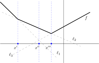
Figure 1. Ordering of local linear functions changes at the boundary between linear regions: $f$ is a CPWL function with local linear functions $\ell_{1}$, $\ell_{2}$ and $\ell_{3}$. Note that $\ell_{1}(x^{\prime})\geq\ell_{2}(x^{\prime})\geq\ell_{3}(x^{\prime})$ and $\ell_{2}(x^{\prime})\geq\ell_{1}(x^{\prime})\geq\ell_{3}(x^{\prime})$ are two different orderings at the boundary point $x^{\prime}$. Also note that the ordering can change within a linear region: c.f. $x^{\prime\prime}$. See also (TarelaRegionConfigurationsRealizability1999, , Figure 1).

This also suggests that we make the following definition, which allows us to talk about regions in the domain of $f$ over which the order of the local linear functions is the same.

Definition 0 (Unique-Order Region (rephrasing of (TarelaRegionConfigurationsRealizability1999, , Definition 2.3))).

Let $f:D\subset\mathbb{R}^{n}\rightarrow\mathbb{R}$ be a CPWL function with $N$ distinct local linear functions $\mathcal{R}=\{\ell_{1},\dots\ell_{N}\}$; that is for all $x\in D$, $f(x)=\ell_{i}(x)$ for some $\ell_{i}\in\mathcal{R}$. Then a unique-order region of $f$ is a region $O\subseteq D$ from the hyperplane arrangement in $\mathbb{R}^{n}$ defined by those hyperplanes $H_{ij}=\{x:\ell_{i}(x)=\ell_{j}(x)\}$ that are non-empty. In particular, for all $x$ in a unique-order region $O$, $\ell_{i_{1}}(x)\geq\ell_{i_{2}}(x)\geq\dots\geq\ell_{i_{N}}(x)$ for some permutation of $i_{k}$ of $\{1,\dots,N\}$.

We are now in a position to describe the two-level lattice representation of a CPWL function.

Theorem 3 (Two-Level Lattice Forms From Unique-Order Regions (TarelaRegionConfigurationsRealizability1999, , Theorem 4.1)).

Let $f$ be as in Definition 2 with $M$ the number of unique-order regions of $f$ in $D$. Then there exists at most $M$ subsets $s_{i}\subseteq\{1,\dots,N\}$, $i=1,\dots,M$ such that:

(22) $$f(x)=\max_{1\leq i\leq M}\min_{j\in s_{i}}\ell_{j}(x)\quad\forall x\in D.$$

3.2. Structure of the Main Algorithm

Having described in detail the lattice representation of a CPWL, we return to the specific claims we made about how it structures our solution to Problem 1.

We first note that the form (22) is well suited to implementation with a ReLU neural network: it is comprised of linear functions and $\max$/$\min$ functions, so many observations from (AroraUnderstandingDeepNeural2016, ) apply to (22) as well. In particular, the two-argument maximum function can be implemented directly with a ReLU using the well-known identity

(23) $$\max\{a,b\}=\frac{a+b}{2}+\frac{|a-b|}{2}$$

and the following ReLU implementations of its constituent expressions (AroraUnderstandingDeepNeural2016, ):

(24) $$|x| =\max\{x,0\}+\max\{-x,0\}$$

(25) $$x =\max\{x,0\}-\max\{-x,0\}.$$

Thus $\max$ can be implemented by a NN ${\mathscr{N}\negthickspace\negthickspace\negthinspace\mathscr{N}}\negthinspace_{\Theta_{\max}}$ where:

(26) $$\Theta_{\max}=(\left[\begin{smallmatrix}1&1\\ -1&-1\\ -1&1\\ 1&-1\end{smallmatrix}\right],\left[\begin{smallmatrix}\frac{1}{2}&-\frac{1}{2}&\frac{1}{2}&\frac{1}{2}\end{smallmatrix}\right])$$

This implementation is illustrated in Figure 2. Using the $\min$ variant of the identity (23), namely:

(27) $$\min\{a,b\}=\frac{a+b}{2}-\frac{|a-b|}{2}$$

leads to a similar ReLU implementation of the two-argument minimum function. In the previous notation, the architectures of these $\max$ and $\min$ networks are the same, i.e. $\text{Arch}(\Theta_{\max})$ = $\text{Arch}(\Theta_{\min})$ = $((2,4),(4,1))$ with no activation function on the last layer.

Figure 2. Illustration of a ReLU network to compute the maximum of two real numbers $a$ and $b$. See also (AroraUnderstandingDeepNeural2016, ).

This implementation further suggests a natural way to implement the multi-element $\max$ (resp. $\min$) operation with a ReLU network (AroraUnderstandingDeepNeural2016, ). Such an operation can be implemented by deploying the two-element $\max$ (resp. $\min$) networks in a “divide-and-conquer” fashion: the elements of the set to be maximized (resp. minimized) are fed pairwise into a layer of two-element $\max$ (resp. $\min$) networks; the output of that first $\max$ (resp. $\min$) layer is fed pairwise into a subsequent layer of two-element $\max$ (resp. $\min$) networks, and so on and so forth until there is only one output. Note that this approach can also be used on sets whose cardinality is not a power of two while maintaining a ReLU structure of the neural network ${\mathscr{N}\negthickspace\negthickspace\negthinspace\mathscr{N}}\negthinspace$: the same value can be directed to multiple inputs as necessary. This structure is illustrated in Figure 3 for a network that computes the maximum of five real-valued inputs. Following this example, an $N$-input $\max$ (or $\min$) network $\max_{N}$ (resp. $\min_{N}$) is represented by a parameter list $\Theta_{{\max}_{N}}$ (resp. $\Theta_{{\min}_{N}}$) which has architecture:

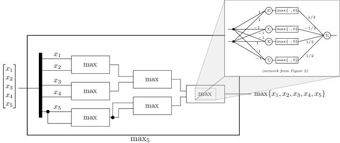
Figure 3. Illustration of a ReLU network to compute the maximum of five real numbers $\{x_{1},x_{2},x_{3},x_{4},x_{5}\}$. Callout depicts the network from Figure 2. See also (AroraUnderstandingDeepNeural2016, ).

(28) $$\text{Arch}(\Theta_{{\max}_{N}})=\text{Arch}(\Theta_{{\min}_{N}})=\\ \Big{(}\;\big{(}N,2\negthinspace\cdot\negthinspace\lceil N/2\rceil\big{)}\;,\;\lceil N/2\rceil\negthinspace\cdot\negthinspace\textnormal{Arch}(\Theta_{\max})\;,\;\hskip 45.0pt\\ (\lceil N/2\rceil-1)\negthinspace\cdot\negthinspace\textnormal{Arch}(\Theta_{\max})\;,\;\dots\;,\;\textnormal{Arch}(\Theta_{\max})\;\Big{)}$$

where $c\cdot\text{Arch}(\Theta_{\max})$ means multiply every element in $\textnormal{Arch}(\Theta_{\max})$ by $c$; nested lists are “flattened” as appropriate; and there is no activation function on the final layer.

Now, given these multi-element $\max$/$\min$ networks, the remaining structure for a ReLU network implementation of the lattice form (22) is clear: we need a neural network architecture capable of (i) implementing $f$’s local linear functions $\mathcal{R}=\{\ell_{1},\dots,\ell_{N}\}$ and (ii) handling the selection of the subsets $s_{i}$. The implementation of the local linear functions is straightforward using a fully connected hidden layer. The selection can be handled by routing – and replicating, as needed – the output of those linear functions to a $\min$ network. Since we do not know the exact size of the subsets $s_{i}$ in (22), and hence the number of input ports for each $\min$ network, we must use $\min$ networks with as many pair-wise $\min$ input ports as there are local linear functions. Then, for subsets $s_{i}$ of size less than $N$, the architecture replicates some local functions multiple times to different input ports of the same $\min$ network to achieve the correct output. As discussed before, such replication does not affect the correctness of the architecture. Moreover, there will be one such $\min$ network for each unique-order region for a total of $M$. This replicating and routing of signals can be accomplished by an auxiliary fully connected linear layer with $N$ inputs and $M\cdot N$ outputs. Since the purpose of this layer is to allow the weights to only select subsets of the local linear functions, this layer should have the property that all of the weights are either zero or one, and each output of the layer should select exactly one input. That is the weight matrix for this layer should have a exactly one $1$ in each row with all of the other weights set to $0$. For a real-valued CPWL function $f:\mathbb{R}^{n}\rightarrow\mathbb{R}$, this overall architecture is depicted in Figure 4. The selection and routing layer is depicted in red. The notation $\mathcal{R}_{\hat{s}_{i}}(x)$ reflects the routing and (one possible) replication of values of the local linear functions, and it is defined as follows:

(29) $$\mathcal{R}_{\hat{s}_{i}}(x)\triangleq\Big{\{}\big{(}\{j\},\ell_{j}(x)\big{)}:j\in s_{i}\Big{\}}\\ \cup\Big{\{}\big{(}\{N+k\},\ell_{\max s_{i}}(x)\big{)}:k=1,\dots,N-|s_{i}|\Big{\}}.$$

(That is $\mathcal{R}_{\hat{s}_{i}}(x)$ contains one copy of each of $\ell_{j}(x):j\in s_{i}$, and as many additional copies of $\ell_{\max s_{i}}(x)$ as necessary to have $N$ total elements. In particular, $\max_{p\in\mathcal{R}_{\hat{s}_{i}}(x)}\pi_{2}(p)=\max_{j\in s_{i}}\ell_{j}(x)$.)

Finally, we note that it is straightforward to extend this architecture to vector-valued functions like $\mu_{\text{MPC}}$. The structure of ${\mathscr{N}\negthickspace\negthickspace\negthinspace\mathscr{N}}\negthinspace$ (Section 2.1) means that a scalar pairwise $\min$ (or $\max$) network can trivially compute the element-wise minimum between two input vectors by simply allowing more inputs and applying the weights from Figure 2 in an element-wise (diagonal) fashion. The result is an architecture that looks exactly like the one in Figure 4, only with the number of outputs $m$ multiplying the size of most signals.

The structure of the above described ReLU implementation is general enough to implement any CPWL function $f$ with $N$ local linear functions and $M$ unique order regions. We state this as a theorem below.

Theorem 4.

Let $f:\mathbb{R}^{n}\rightarrow\mathbb{R}$ by CPWL with distinct local linear functions $\mathcal{R}=\{\ell_{1},\dots,\ell_{N}\}$ and $M$ unique order regions. Then there is a parameter list $\Theta_{N,M}$ with:

(30) $$\textnormal{Arch}(\Theta_{N,M})=\\ \Big{(}\;\underbrace{(n,N\cdot M)}_{\text{linear layer}},\;\underbrace{M\cdot\textnormal{Arch}(\Theta_{\min_{N}})}_{\min\text{ layer}}\;,\;\underbrace{\textnormal{Arch}(\Theta_{\max_{M}})}_{\max\text{ layer}}\;\Big{)}$$

such that there exist an assignments for $\Theta_{N,M}$ that renders:

$${\mathscr{N}\negthickspace\negthickspace\negthinspace\mathscr{N}}\negthinspace_{\Theta_{N,M}}(x)=f(x)\qquad\forall x\in\mathbb{R}^{n},$$

where $M\cdot\textnormal{Arch}(\Theta_{\min_{N}})$ means multiply every element in $\textnormal{Arch}(\Theta_{\min_{N}})$ by $M$, and where nested lists are “flattened” as needed. The final layers of the $\min$ layer and the $\max$ layer lack activation functions.

Proof.

The proof is constructive: the discussion above explains the construction, which is based on (TarelaRegionConfigurationsRealizability1999, , Theorem 4.1). ∎

Corollary 0.

Any CPWL controller $\mu$ (such as $\mu_{\text{MPC}}$) can be implemented by a ReLU network $\Theta$ with architecture $\textnormal{Arch}(\Theta_{N,M})$ as described in Theorem 4, where $N$ is the number local linear functions of $\mu$ and $M$ is the number of unique-order regions of $\mu$.

Note that in many cases it is hard to exactly know the parameters $N$ and $M$ exactly. The next result show that our correctness claims in Theorem 2 can be extended when an upper bound $\mkern 3.0mu\overline{\mkern-2.5muN\mkern-2.0mu}\mkern 2.0mu\geq N$ and $\mkern 3.0mu\overline{\mkern-2.5muM\mkern-2.0mu}\mkern 2.0mu\geq M$ is used to design the neural network architecture as explained in the next result.

Theorem 6.

Let $\Theta_{N,M}$ be a parameter list such that $\textnormal{Arch}(\Theta_{N,M})$ is as specified in Theorem 4, (30), and let $\mkern 3.0mu\overline{\mkern-2.5muN\mkern-2.0mu}\mkern 2.0mu\geq N$ and $\mkern 3.0mu\overline{\mkern-2.5muM\mkern-2.0mu}\mkern 2.0mu\geq M$. Then there exists a parameter list $\Theta_{\mkern 3.0mu\overline{\mkern-2.5muN\mkern-2.0mu}\mkern 2.0mu,\mkern 3.0mu\overline{\mkern-2.5muM\mkern-2.0mu}\mkern 2.0mu}$ with $\textnormal{Arch}(\Theta_{\mkern 3.0mu\overline{\mkern-2.5muN\mkern-2.0mu}\mkern 2.0mu,\mkern 3.0mu\overline{\mkern-2.5muM\mkern-2.0mu}\mkern 2.0mu})$ as in (30) such that:

(31) $${\mathscr{N}\negthickspace\negthickspace\negthinspace\mathscr{N}}\negthinspace_{\Theta_{N,M}}(x)={\mathscr{N}\negthickspace\negthickspace\negthinspace\mathscr{N}}\negthinspace_{\Theta_{\mkern 3.0mu\overline{\mkern-2.5muN\mkern-2.0mu}\mkern 2.0mu,\mkern 3.0mu\overline{\mkern-2.5muM\mkern-2.0mu}\mkern 2.0mu}}(x)\quad\forall x.$$

Proof.

In order to implement the same function with a larger network, the extra linear-layer neurons can simply duplicate calculations carried out by neurons in the smaller network. For example, the extra neurons in the the first linear layer can duplicate the calculation of $\ell_{N}$, and the extra neurons in the second linear layer can duplicate the calculation of the $M^{\text{th}}$ subset of $\{\ell_{1},\dots,\ell_{N}\}$. This will not change the output of the $\min$ and $\max$ layers. ∎

Note: when “embedding” a smaller network, $\Theta_{N,M}$, into a larger one, $\Theta_{\mkern 3.0mu\overline{\mkern-2.5muN\mkern-2.0mu}\mkern 2.0mu,\mkern 3.0mu\overline{\mkern-2.5muM\mkern-2.0mu}\mkern 2.0mu}$, it is incorrect to set the extra parameters in $\Theta_{\mkern 3.0mu\overline{\mkern-2.5muN\mkern-2.0mu}\mkern 2.0mu,\mkern 3.0mu\overline{\mkern-2.5muM\mkern-2.0mu}\mkern 2.0mu}$ to zero, as this could affect the output of the $\min$ and $\max$ networks!

Thus, to use this framework to obtain an architecture that is capable of implementing $\mu_{\text{MPC}}$, one needs to simply upper-bound the number of local linear functions $N$ in $\mu_{\text{MPC}}$ (ultimately without solving the actual MPC problem) and upper-bound the number of unique order regions $M$ in $\mu_{\text{MPC}}$. This is precisely the AReN algorithm, as specified in Algorithm 1. The constituent functions EstimateRegionCount and EstimateUniqueOrder are described in detail in the subsequent sections Section 4 and Section 5, respectively. The implementation of the function InferArchitecture follows directly from the (constructive) discussion in this section.

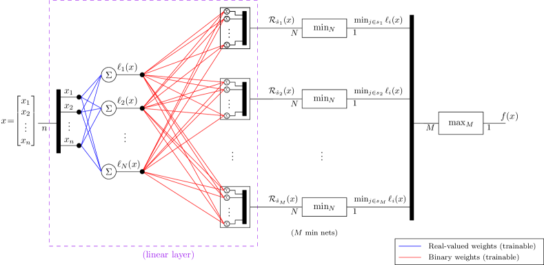
Figure 4. Illustration of the overall architecture to implement a scalar CPWL function. The symbols for various signals are indicated above the line, and their dimensions are indicated below the line. The red lines represent a fully-connected linear layer in which the weights flowing into a single summer have the property that exactly one of them is equal to $1$, and the others are all $0$. $\mathcal{R}_{\hat{s}_{i}}(x)$ is defined in (29).

input : system matrices $A$,$B$,$C$; cost matrices $P,Q\geq 0$, $R>0$; feedback matrix $K$; horizon $N_{c}$

output : $(K,\dim(\theta^{(1)}_{1}),\dots,\dim(\theta^{(K)}_{1}))$

1 function GetArchitecture(A,B,C,P,Q,R,K,$\text{N}_{\text{c}}$)

2       N_est $\leftarrow$ EstimateRegionCount(A,B,C,P,Q,R,K,$\text{N}_{\text{c}}$)

3      M_est $\leftarrow$ EstimateUniqueOrderCount(N_est)

4      ArchList $\leftarrow$ InferArchitecture(N_est,M_est)

5      return ArchList

6 end

Algorithm 1 AReN.

4. Approximating the number of linear regions in the MPC controller

In this section, we will discuss our implementation of the function EstimateRegionCount from Algorithm 1. A natural means to approximate to the number of local linear functions of $\mu_{\text{MPC}}$ is to approximate the number of maximal linear regions in $\mu_{\text{MPC}}$.

Definition 0 (Linear Region of $\mu_{\text{MPC}}$).

A linear region of $\mu_{\text{MPC}}$ is a subset of $\mathscr{R}\subseteq\mathbb{R}^{n}$ over which $\mu_{\text{MPC}}(x)=L(x)$ for some linear (affine) $L:\mathbb{R}^{n}\rightarrow\mathbb{R}^{m}$. A maximal linear region is a linear region that is strictly contained in no other linear regions. Two linear regions are said to be distinct if they correspond to different linear functions, $L$.

Thus, the maximal linear regions of $\mu_{\text{MPC}}$ are in one-to-one correspondence with the local linear functions in $\mu_{\text{MPC}}$ (Definition 1), so an upper bound on the number of maximal linear regions in $\mu_{\text{MPC}}$ is an upper bound on its number of local linear function, which in turn will provide an over-approximation of $N$ that can be used to generate a NN architecture.

To upper bound the number of maximal linear regions effectively, we need to consider in detail some specifics about how the piecewise linear property arises in the solution for $\mu_{\text{MPC}}$. Ultimately, $\mu_{\text{MPC}}$ is piecewise linear because we have posed a problem for which (i) the gradient of the Lagrangian (34) is linear in both the Lagrange multipliers and the decision variable; and (ii) the dependence on the initial state $x(t)$ is linear. Linearity is important in both (i) and (ii) because we are really not solving one optimization problem but a family of them: one for each initial state $x(t)$. Thus, the linearity of the Lagrangian together with the linearity of the inequality constraints in $x(t)$ leads to an equation (a necessary optimality condition) that is linear in both the Lagrange multipliers and the initial state $x(t)$: hence the piecewise-linear controller $\mu_{\text{MPC}}$.

Moreover, the distinct linear regions of $\mu_{\text{MPC}}$ – i.e. those with distinct linear functions – arise out of a particular aspect of the aforementioned linear equations. In particular, the Lagrange multipliers, $\lambda$, and the initial state, $x(t)$, appear together in a linear equation that has different solutions – and hence creates different linear regions for $\mu_{\text{MPC}}$ – based on which of the inequality constraints are active (at a particular optimizer) (BemporadExplicitLinearQuadratic2002, , Theorem 2). Since the linear regions obtained in this way partition the domain of $\mu_{\text{MPC}}$ (see also Proposition 3 below), this suggests that we can over-approximate the number of linear regions in $\mu_{\text{MPC}}$ by counting all of the possible constraints that can be active at the same time. Indeed, this is more or less how EstimateRegionCount arrives at an estimate for $N$, although we do not simply over-approximate with $2^{\text{\# of constraints}}$.

4.1. The Optimal MPC Controller

As preparation for the rest of the section, we begin by summarizing some further details regarding the solution of $\mu_{\text{MPC}}$ from (BemporadExplicitLinearQuadratic2002, ). In particular, the optimization problem specified by (7)-(16) can be simplified by directly substituting the dynamics constraint (14) to get:

(32) $$\min_{U}\left\{\frac{1}{2}x(t)^{\text{T}}\;Y\;x(t)+\frac{1}{2}U^{\text{T}}\;H\;U+x(t)^{\text{T}}\;F\;U\right\}$$

$$\text{subject to: }\qquad\quad GU\leq W+Ex(t)$$

with appropriately defined matrices $H$, $F$, $G$, $W$ and $E$ of dimensions $(\rho\times\rho)$, $(n\times\omega)$, $(\rho\times\omega)$, $(\rho\times 1)$ and $(\rho\times n)$, respectively (where $\omega$ and $\rho$ are defined in (17) and (18), respectively). Then, completing the square by means of the change of variables $z\triangleq U+H^{-1}F^{\text{T}}x(t)$ provides the following, simplified quadratic program (BemporadExplicitLinearQuadratic2002, ):

(33) $$\min_{z}\left\{\frac{1}{2}z^{\text{T}}\;H\;z\right\}\quad\text{ subject to: }\quad Gz\leq W+Sx(t).$$

Note that this change of variables is only valid when $H$ is invertible, but this is assumed in (BemporadExplicitLinearQuadratic2002, ), and it will be assumed throughout.

A solution to the optimization problem in (33) can be easily formulated using the KKT (necessary) optimality conditions (LuenbergerOptimizationVectorSpace1997, ). This results in the following system of equations:

(34) $$Hz+G^{\text{T}}\lambda =0\qquad\lambda\in\mathbb{R}^{\rho}$$

(35) $$\lambda_{i}(G_{i}z-W_{i}-S_{i}x) =0\qquad i\in 1\ldots\rho$$

(36) $$\lambda \geq 0$$

(37) $$Gz \leq W+Sx.$$

That is for a (local) minimizer to the optimization problem (33), there exists non-negative Lagrange multipliers $\lambda$ that solve the above system. Moreover, solving (34) for the minimizer, $z$, demonstrates that such a minimizer has a particular structure. Indeed, under the assumption that $H$ is invertible, we may solve (34) for $z$ and substituted it into (37) to obtain:

(38) $$-GH^{-1}G^{\text{T}}\lambda\leq W+Sx.$$

Now given the relevance of active constraints in (34) - (37) to(BemporadExplicitLinearQuadratic2002, , Theorem 2), we introduce the following notation.

Definition 0 (Selector Matrix).

Let $\alpha\subseteq\{1,\dots,\rho\}$, and define the auxiliary set (and associated vector):

$$\tilde{\alpha} \triangleq\{(1,\min_{j\in\alpha}j),\dots,(|\alpha|,\max_{j\in\alpha}j)\}.$$

Then the selector matrix, $\tilde{I}_{\alpha}$ is defined as:

(39) $$\tilde{I}_{\alpha}\triangleq[e_{\tilde{\alpha}(1)},\dots,e_{\tilde{\alpha}(|\alpha|)}]^{\text{T}}$$

where $e_{j}$ is the $j^{\text{th}}$ column of the $(\rho\times\rho)$ identity matrix.

The selector matrix can thus be used to describe equality in (38) for the active constraints by removing inequalities associated with the inactive constraints. In particular, given a set of active constraints specified by a subset $\alpha\subseteq\{1,\dots,\rho\}$, the Lagrange multipliers for the active constraints, $\lambda_{\alpha}$, will satisfy the following:

(40) $$-\tilde{I}_{\alpha}G(H^{-1}G^{\text{T}}\tilde{I}_{\alpha}^{\text{T}})\lambda_{\alpha}=\tilde{I}_{\alpha}(W+Sx).$$

In particular, (40) is a linear equation in $\lambda_{\alpha}$ and $x$ that ultimately specifies the region in $x$-space over which a single affine function characterizes $\mu_{\text{MPC}}$. Indeed, back substituting solutions of (40) into (37) and $\lambda\geq 0$ specifies a set of linear inequalities in $x$. These equivalently define an intersection of half-spaces in $\mathbb{R}^{n}$ that characterize a (convex) linear region of $\mu_{\text{MPC}}$ (BemporadExplicitLinearQuadratic2002, , Theorem 2). Moreover, since every possible solution to the optimization problem admits some set of active constraints, these convex linear regions partition the state space.

For our purposes, (40) is the relevant consequence of this discussion, since it most readily suggests how to over-approximate the number of linear regions of $\mu_{\text{MPC}}$. We describe how to do this in the next subsection.

4.2. Over-approximating the Number of Maximal Linear Regions

From the previous discussion, the problem of finding all possible sets of active constraints for (34) - (37) is a significant amount of the work in solving for the optimal controller $\mu_{\text{MPC}}$. However, we are content not solving for $\mu_{\text{MPC}}$ exactly: thus, we only need to simplify (40) in such a way that we obtain a new equation with all of the same solutions plus some spurious ones (keep in mind that (40) is an equation in $\alpha$, too).

Before we begin counting regions, we need to state the following proposition, which is trivial given the observations in (BemporadExplicitLinearQuadratic2002, ).

Proposition 0.

Let $\bar{\mathscr{R}}$ be a maximal linear region for controller $\mu_{\text{MPC}}$. Then there exists a finite collection of sets $\Gamma_{\bar{\mathscr{R}}}=\{\alpha_{i}\subseteq\{1,\dots,\rho\}:i=1,\dots V\}$ with the following property:

• for every $x\in\bar{\mathscr{R}}$, there exists an $\alpha_{x}\in\Gamma$ and $|\alpha_{x}|$ Lagrange multipliers $\lambda_{\alpha_{x}}\geq 0$ such that:

  (41) $$\tilde{I}_{\alpha_{x}}GH^{-1}G^{\text{T}}\tilde{I}_{\alpha_{x}}^{\text{T}}\lambda_{\alpha_{x}}=\tilde{I}_{\alpha_{x}}(W+Sx).$$

In particular, any maximal linear region of $\mu_{\text{MPC}}$ can be partitioned into $|\Gamma|$ convex linear regions.

Proof.

Since we are considering a maximal linear region of $\mu_{\text{MPC}}$, the quadratic program (33) is feasible for every $x\in\bar{\mathscr{R}}$ by definition. Consequently, there is for every such $x$, a unique solution $z^{*}_{x}$, and so by necessity, there is some set of constraints $\alpha_{x}\subseteq\{1,\dots,\rho\}$ that is active at $z^{*}_{x}$. Moreover, by the KKT necessary conditions, there exists $|\alpha|$ Lagrange multipliers $\lambda_{\alpha_{x}}$ that satisfy (41). This proves the existential assertions for $x\in\bar{\mathscr{R}}$ related to (41).

However, we have implicitly defined a function that associates to each $x\in\bar{\mathscr{R}}$ a subset in $2^{\{1,\dots,\rho\}}$:

$$\textnormal{act}:\mathbb{R}^{n} \rightarrow 2^{\{1,\dots,\rho\}}$$

(42) $$x \mapsto\alpha_{x}.$$

We define $\Gamma_{\bar{\mathscr{R}}}=\textnormal{act}(\bar{\mathscr{R}})$ to be the range of act, so that equivalence modulo act partitions $\bar{\mathscr{R}}$ into $|\Gamma|$ disjoint regions. Finally, by (BemporadExplicitLinearQuadratic2002, , Theorem 2) and the discussion about degeneracy on (BemporadExplicitLinearQuadratic2002, , pp. 9), each of these regions is necessarily convex. ∎

Proposition 3 gives us a hint about how to over-approximate the number of maximal linear regions: in particular, we will simplify equation (41) in such a way that we still find solutions for each $\alpha\in\Gamma$ at the expense of including solutions for $\alpha\not\in\Gamma$. This gives us our first main counting theorem:

Theorem 4.

Let $\Xi\subseteq 2^{\{1,\dots,\rho\}}\backslash\emptyset$ such that for every $\alpha\in\Xi$ there exists a vector $\eta_{\alpha}\in\mathbb{R}^{\rho}$ such that:

(43) $$GH^{-1}G^{\text{T}}\tilde{I}_{\alpha}\lambda_{\alpha}=\eta_{\alpha}.$$

has a solution $\lambda_{\alpha}\geq 0$, $\lambda_{\alpha}\neq 0$. Then $|\Xi|+1$ upper bounds the number of maximal linear regions for $\mu_{\text{MPC}}$.

Proof.

If we show that for every maximal linear region $\bar{\mathscr{R}}$, the $\Gamma_{\bar{\mathscr{R}}}\subseteq\Xi\cup\emptyset$, then the conclusion will follow.

But this follows directly from Proposition 3: for each $\alpha\in\Gamma_{\bar{\mathscr{R}}}$, there exists an $x$ and $\alpha=\lambda_{\alpha_{x}}$ such that (41) holds. Thus if $\lambda_{\alpha}=\lambda_{\alpha_{x}}$ and $\lambda_{\alpha_{x}}\neq 0$, then set $\alpha=\alpha_{x}$, $\eta_{\alpha}=W+Sx$ and conclusion holds. The situation when no constraints are active is accounted for with the addition of $1$ in the final conclusion. ∎

Theorem 4 is significant because Farkas’ lemma (LuenbergerOptimizationVectorSpace1997, ) tells us how to describe the solutions of (43) using a linear inequality feasibility problem. In particular, (43) has a non-trivial solution if and only if the problem $(GH^{-1}G^{\text{T}}\tilde{I}_{\alpha}^{\text{T}})^{\text{T}}\chi\leq 0$ is feasible (and it can’t have only the trivial solution for non-trivial $\lambda_{\alpha}$). This reasoning is included in the proof of the subsequent Theorem, which connects the bound from Theorem 4 to the number of feasible “sub-problems” defined by $GH^{-1}G^{\text{T}}$. First, we introduce the following definition.

Definition 0 (Non-trivially Feasible).

Let $V$ be a $(\rho\times\rho^{\prime})$ matrix and let $\alpha\subseteq\{1,\dots,\rho\}$. Then $\alpha$ is a non-trivially feasible subset of $V$ if there exists a $\chi\in\mathbb{R}^{\rho^{\prime}}$, $\chi\neq 0$ such that $I_{\alpha}V\chi\geq 0$. Such a set is maximal if adding any other row makes it infeasible.

Now we state the main theorem in this section.

Theorem 6.

Let $\mathscr{I}$ be the set of maximal non-trivially feasible subsets of $GH^{-1}G^{\text{T}}$ (see Definition 5). Then the number of maximal linear regions in $\mu_{\text{MPC}}$ is bounded above by:

(44) $$\Big{|}\bigcup_{\alpha\in\mathscr{I}}2^{\alpha}\Big{|}\leq\sum_{\alpha\in\mathscr{I}}2^{|\alpha|}.$$

Proof.

This follows from Farkas’ lemma and Theorem 4.

In particular, let $\alpha\subseteq\{1,\dots,\rho\}$ and $\eta_{\alpha}\neq 0\in\mathbb{R}^{\rho}$. Now, by Farkas’ lemma,

(45) $$\exists\lambda_{\alpha}\geq 0\;.\;GH^{-1}G^{\text{T}}\tilde{I}_{\alpha}\lambda_{\alpha}^{\text{T}}=\eta_{\alpha}\Leftrightarrow\\ \exists\chi\in\mathbb{R}^{\rho}\text{ s.t. }\eta_{\alpha}^{\text{T}}\chi<0\text{ and }\tilde{I}_{\alpha}(GH^{-1}G^{\text{T}})^{\text{T}}\chi\leq 0.$$

In particular, $GH^{-1}G^{\text{T}}\tilde{I}_{\alpha}\lambda_{\alpha}^{\text{T}}=\eta_{\alpha}$ can have a non-negative solution if and only if $\alpha$ is a non-trivially feasible subset of $(GH^{-1}G^{\text{T}})^{\text{T}}$.

Thus, by Theorem 4, we conclude that $\alpha\in\Xi$ implies $\alpha$ is a non-trivially feasible subset of $(GH^{-1}G^{\text{T}})^{\text{T}}$, and hence, that the number of maximal linear regions is bounded by the number of non-trivially feasible subsets of $GH^{-1}G^{\text{T}}$. The conclusion of the theorem thus follows because every non-trivially feasible subset is a subset of some maximally non-trivially feasible subset. ∎

4.3. Implementing EstimateRegionCount

To find maximal non-trivially feasible subsets of $GH^{-1}G^{T}$, we start by introducing one Boolean variable $b_{i}$ for each column of the matrix $GH^{-1}G^{T}$. The first non-trivially feasible subset can then be found by solving the following problem:

(46) $$\text{arg}\max_{(b_{1},\ldots,b_{\rho},\lambda)\in\mathbb{B}^{\rho}\times\mathbb{R}^{\omega}}\sum_{i=1}^{\rho}b_{i}$$

(47) $$\text{subject to}\qquad b_{i}\Rightarrow[GH^{-1}G^{T}]_{i}\lambda<0,\;\;i=1,\ldots,\rho$$

where $[GH^{-1}G^{T}]_{i}$ denotes the $i$th column of the matrix $GH^{-1}G^{T}$. Such optimization problems can be solved efficiently using Satisfiability Modulo Convex programming (SMC) solvers (shoukry2018smc, ; shoukry2017smc, ). SMC solvers first use a pseudo-Boolean Satisfiability (SAT) solver to find a valuation of the Boolean variables that maximizes the objective function (46); this is then followed by a linear programming (LP) solver that finds solutions to the constraints in (47). Indeed, the SAT solver may return an assignment for the Boolean variables $b_{1},\ldots,b_{\rho}$ for which the corresponding LP problem is infeasible. In such a case, we use the LP solver to search for a set of Irreducibly Infeasible Set (IIS) that explains the reason behind such infeasibility. This IIS is then encoded into a constraint that prevents the SAT solver from returning any assignment that can lead to the same IIS. We iterate between the SAT solver and the LP solver until one Boolean assignment is found for which the corresponding LP problem is feasible. It follows from maximizing the objective function that this set of active constraints is guaranteed to be a maximal non-trivially feasible subset of $GH^{-1}G^{T}$.

Once a maximal non-trivially feasible subset of $GH^{-1}G^{T}$ is found, we can add a blocking Boolean constraints to the SAT solver, thus preventing the SAT solver from producing any subsets of this maximal non-trivially feasible set. We continue this process until the SAT solver can not find any more feasible assignments to the Boolean variables, at which point our algorithm terminates and returns all of the non-trivially feasible subsets it has obtained. This discussion is summarized in Algorithm 2 whose correctness follows from the correctness of SMC solvers (shoukry2018smc, ; shoukry2017smc, ).

1

2

3

4

input : system matrices $A$,$B$,$C$; cost matrices $P,Q\geq 0$, $R>0$; feedback matrix $K$; horizon $N_{c}$

output : N_est

5 function EstimateRegionCount(A,B,C,P,Q,R,K,$\text{N}_{\text{c}}$)

6       G_Hinv_Gtr $\leftarrow$ GetHyperplanes(A,B,C,P,Q,R,K,$\text{N}_{\text{c}}$)

7      NumHyperplanes $\leftarrow$ Dimensions(G_Hinv_Gtr)[0]

8      $($ h $\negthinspace[1],\dots,$ h $\negthinspace[\texttt{NumHyperplanes}]~{})$ $\leftarrow$ G_Hinv_Gtr

9      $($ b $\negthinspace[1],\dots,$ b $\negthinspace[\texttt{NumHyperplanes}]~{})$ $\leftarrow$ createBooleanVariables(NumHyperplanes)

10      Solutions $\leftarrow$ ( ) ; SATConstraints $\leftarrow$ ( )

11      while True do

12             SATsolver.setConstraints(SATConstraints)

13            SATsolver.Maximize($\sum_{i=1}^{{\textnormal{{NumHyperplanes}}}}$ b $\negthinspace[i]$)

14            if not SATsolver.SAT?() then

15                   break

16             end if

17            

18            HyperplaneSet $\leftarrow$ G_Hinv_Gtr.

19                     GetHyperplanes(SATsolver.TrueVars())

20            Feasible? $\leftarrow$ CheckFeasibility(HyperplaneSet *z $\leq-\varepsilon$)

21            if not Feasible? then

22                  

23                  IIS $\leftarrow$ GetIIS(HyperplaneSet)

24                  SATConstraints.Append( $\bigvee_{\texttt{h}[i]\in{\textnormal{{IIS}}}}\neg{\texttt{b}}[i]$ )

25            else

26                   Solutions.Append(HyperplaneSet)

27                  SATConstraints.Append (

28                  $\quad\sum_{\texttt{h}[i]\in{\texttt{HyperplaneSet}}}\negthinspace{\texttt{b}}[i]\negthinspace<\negthinspace|\textnormal{{HyperplaneSet}}|\negthinspace\Rightarrow$

29                  $\qquad\quad\sum_{\texttt{h}[i]\not\in{\textnormal{{HyperplaneSet}}}}{\texttt{b}}[i]\geq 1$

30                  )

31             end if

32            

33       end while

34      

35      return N_est $\leftarrow$ CountAllUniqueSubsets(Solutions)

36 end

Algorithm 2 EstimateRegionCount.

5. Approximating the Number of Unique-Order Regions in the MPC Controller

In this section, we discuss our implementation of EstimateUniqueOrder from Algorithm 1. Unlike our implementation of EstimateRegionCount, which we could base of aspects of the MPC problem, the implementation of this function merely exploits a general bound on the number of possible regions in an arrangement of hyperplanes.

In particular, we noted in Definition 2 that the unique-order regions created by a set of local linear functions $\mathcal{R}=\{\ell_{1},\dots,\ell_{N}\}$ correspond to the regions in the hyperplane arrangement specified by non-empty hyperplanes of the form $H_{ij}=\{x:\ell_{i}(x)=\ell_{j}(x)\}$, each of which is a hyperplane in dimension of $n$ (when $x\in\mathbb{R}^{n}$).

There seems to be a well-known – but rarely stated – upper bound on the number of regions that can be formed by a hyperplane arrangement of $N$ hyperplanes in dimension $n$. The few places where it is stated (e.g (SerraBoundingCountingLinear2018, , Lemma 4)) seem to ambiguously quote Zaslavsky’s Theorem (StanleyIntroductionHyperplaneArrangements, , Thoerem 2.5) in their proofs. Thus, we state the bound, and sketch a proof.

Theorem 1.

Let $\mathcal{A}$ be an arrangement of $N$ hyperplanes in dimension $n$. Then the number of regions created by this arrangement, $r(\mathcal{A})$ is bounded by:

(48) $$r(\mathcal{A})\leq\sum_{i=0}^{n}{N\choose i}$$

(with equality if and only if $\mathcal{A}$ is in general position (StanleyIntroductionHyperplaneArrangements, , pp. 4)).

Proof.

First, we note that the bound holds with equality for arrangements in general position (defined on (StanleyIntroductionHyperplaneArrangements, , pp. 4)); this is from (StanleyIntroductionHyperplaneArrangements, , Proposition 2.4), a consequence of Zaslavsky’s theorem (StanleyIntroductionHyperplaneArrangements, , Theorem 2.5). Thus, the claim holds if every other arrangement has fewer regions than an arrangement in general position with the same number of hyperplanes.

This is indeed the case, but it helps to have a little bit of terminology first. In particular, we introduce the general formula for the number of regions in a hyperplane arrangement, $r(\mathcal{A})$, in terms of a triple of hyperplane arrangements $(\mathcal{A},\mathcal{A}^{\prime},\mathcal{A}^{\prime\prime})$ (StanleyIntroductionHyperplaneArrangements, , pp. 13), namely (StanleyIntroductionHyperplaneArrangements, , Lemma 2.1):

(49) $$r(\mathcal{A})=r(\mathcal{A}^{\prime})+r(\mathcal{A}^{\prime\prime}).$$

Such a triple is formed by choosing a distinguished hyperplane $H_{d}\in\mathcal{A}$, and defining $\mathcal{A}^{\prime}$ as $\mathcal{A}\backslash\{H_{d}\}$ and $\mathcal{A}^{\prime\prime}$ as the arrangement of hyperplanes $\{H\cap H_{d}\neq\emptyset:H\in\mathcal{A}^{\prime}\}$. Note that $\mathcal{A}^{\prime\prime}$ characterizes the regions in $\mathcal{A}^{\prime}$ that are split by $H_{d}$.

From here, we will only provide a brief proof sketch. The proof proceeds by induction: first on the number of hyperplanes in $n=2$, and then on by induction on the dimension, $n$. For $n=2$, the result can be shown for arrangements of size $N$ using (49), and noting that $r(\mathcal{A}^{\prime\prime})=N$ if and only if $H_{d}$ intersects all the other hyperplanes exactly once. This, together with the induction assumption, shows $r(\mathcal{A})$ can satisfy the claim with equality only if $\mathcal{A}$ is in general position. For $n>2$, the proof proceeds similarly, using (49) to invoke the conclusion for $n-1$ as necessary. ∎

Thus, our implementation of EstimateUniqueOrderCount simply computes and returns the value in (48). In the worst case, this estimate is $2^{\text{\# of hyperplanes}}$: this occurs for example when $N=n$. But for $N>>n$, this bound clearly grows more slowly than exponentially in $N$. This is extremely helpful in keeping the size of the second linear layer in Figure 4 of a reasonable size.

We conclude this section by noting that the result in Theorem 1 may be used to state Theorem 6 independently of $M$ entirely. In particular, we have the following theorem.

Theorem 2.

Let $f$ be a CPWL function, and let $\mkern 3.0mu\overline{\mkern-2.5muN\mkern-2.0mu}\mkern 2.0mu$ be an upper-bound on the number of local linear functions in $f$. Then for $M^{\prime}=\sum_{i=0}^{n}{N\choose i}$ there exists a parameter list $\Theta_{\mkern 3.0mu\overline{\mkern-2.5muN\mkern-2.0mu}\mkern 2.0mu,M^{\prime}}$ with $\textnormal{Arch}(\Theta_{\mkern 3.0mu\overline{\mkern-2.5muN\mkern-2.0mu}\mkern 2.0mu,M^{\prime}})$ as in (30) such that:

(50) $$f(x)={\mathscr{N}\negthickspace\negthickspace\negthinspace\mathscr{N}}\negthinspace_{\Theta_{\mkern 3.0mu\overline{\mkern-2.5muN\mkern-2.0mu}\mkern 2.0mu,M^{\prime}}}(x)\quad\forall x.$$

6. Discussion: Hinging Hyperplane Implementations

For comparison, we will make some remarks about the hinging hyperplane representation used in (AroraUnderstandingDeepNeural2016, , Theorem 2.1).

Theorem 1 (Hinging Hyperplane Representation (ShuningWangGeneralizationHingingHyperplanes2005, )).

Let $f:\mathbb{R}^{n}\rightarrow\mathbb{R}$ be a CPWL function. Then there exists a finite integer $K$ and $K$ non-negative integers $\{\eta_{k}:k=1,\ldots,K\}$, each less than $n+1$, such that

(51) $$f(x)=\sum_{k=1}^{K}\sigma_{k}\max\left\{\mathcal{L}^{(k)}_{1}(x),\mathcal{L}^{(k)}_{2}(x),\ldots,\mathcal{L}^{(k)}_{\eta_{k}}(x)\right\}\quad\forall x\in\mathbb{R}^{n}$$

for some collection of $\mathcal{L}^{(k)}_{i}$, $i\in\{1,\ldots,\eta_{k}\}$, each of which is an affine function of its argument $x$, and each constant $\sigma_{k}\in\{-1,+1\}$. (Each $\mathcal{L}^{(k)}_{i}$ beyond the first one is referred to as a “hinge”. That is $\eta_{k}-1$ is the number of “hinges” in the $k^{\text{th}}$ summand.)

The problem with creating a NN architecture from Theorem 1 is that its proof provides only an existential assertion – by means of explicit construction – and that construction relies heavily on particular knowledge of the actual local linear functions in the CPWL (ShuningWangGeneralizationHingingHyperplanes2005, , Theorem 1). Thus, the number $K$ in (51) – which is essentially the only architectural parameter in the ReLU – has a complicated dependence on the particular CPWL function (see (ShuningWangGeneralizationHingingHyperplanes2005, , Corollary 3) as it appears in the proof of (ShuningWangGeneralizationHingingHyperplanes2005, , Theorem 1)). This even makes it difficult to “replay” the proof of Theorem 1 and upper-bound the size of the existential assertions in each step as necessary; there are naive upper bounds for each step, but they lead to an extravagant number of $\max$ operations (exponentially many, in fact).

Moreover, a further complication is that hinging hyperplane representations need not even be unique. For example, consider $f(x)=|x|$: for this function, $K=1$ works because $|x|=\max\{x,-x\}$. But the same function could also be implemented as

(52) $$|x|=\max\{-x,3x+4\}-\max\{0x,4x+4\}+\max\{0x,2x\}$$

which has $K=3$ and five different linear functions $\mathcal{L}$. However, this clearly suggests an alternate approach to upper-bounding the steps in Theorem 1: create an architecture derived from the CPWL with the largest minimal hinging-hyperplane representation. We conjecture that such a maxi-min hinging hyperplane form would in fact lead to fewer $\max$ units than the lattice representation used in AReN. Unfortunately, as far as we are aware, there exists no such minimal characterization in the literature (as a function of the number of local linear functions, say), so we leave consideration of this problem to future work.

7. Numerical Results

The function EstimateRegionCount (Algorithm 2) is the bottleneck in Algorithm 1. Therefore, we chose to benchmark Algorithm 2 to gage the overall performance of our proposed framework. We implemented EstimateRegionCount using SAT solver Z3 and convex solver CPLEX using their respective Python interfaces. We tested our implementation on single-input,single-output MPC problems in two contexts: (1) with a varying number of states; and (2) with a varying prediction horizon $N_{c}$. The computer used had an Intel Core i7 2.9-GHz processor and 16 GB of memory.

Figure 5 (top) shows the performance of Algorithm 2 as a function of the number of plant states, $n$, with all other parameters held constant. The estimated number of local linear functions N_est output by EstimateRegionCount is plotted on one axis; the maximum number of linear functions needed, $2^{\rho}$, is also shown for reference. The other axis shows the execution time for each problem in seconds. It follows from Theorem 6 that the number of plant states doesn’t change the number of constraints and hence does not contribute to the complexity of Algorithm 2. Note that Algorithm 2 reported a number of local linear functions that is one order of magnitude less than the maximum number of linear functions needed, $2^{\rho}$ while taking less than 1.5 minutes of execution time.

Figure 5 (bottom) shows the performance of our algorithm (in semi-log scale) as a function of the number of constraints, $\rho$, with all other parameters held constant ($n=100$). The estimated number of linear functions output by EstimateRegionCount is plotted on one axis; the maximum number of linear functions needed, $2^{\rho}$, is also shown for reference. The other axis shows the execution time for each problem in seconds. Again, we notice an order of magnitude difference between the reported number of local linear functions versus the maximum number of linear functions needed, $2^{\rho}$. Indeed, the execution time is affected by increasing the number of constraint, nevertheless, Algorithm 2 terminates in less than 1.5 hours for a system with more than 300,000 maximal linear regions.

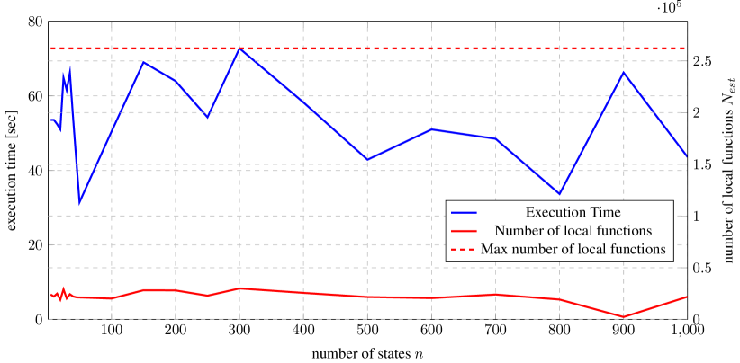
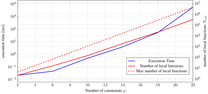
Figure 5. Execution time results: (top) when the number of states $n$ increases for a fixed number of constraints and (bottom) when the number of constraints $\rho$ increases for a fixed number of states $n=100$.

References

- [1] Bernt M Akesson and Hannu T Toivonen. A neural network model predictive controller. Journal of Process Control, 16(9):937–946, 2006.
- [2] Brandon Amos, Ivan Jimenez, Jacob Sacks, Byron Boots, and J Zico Kolter. Differentiable mpc for end-to-end planning and control. In Advances in Neural Information Processing Systems, pages 8289–8300, 2018.
- [3] Raman Arora, Amitabh Basu, Poorya Mianjy, and Anirbit Mukherjee. Understanding Deep Neural Networks with Rectified Linear Units. 2016.
- [4] Bowen Baker, Otkrist Gupta, Nikhil Naik, and Ramesh Raskar. Designing neural network architectures using reinforcement learning. arXiv:1611.02167, 2016.
- [5] Alberto Bemporad, Manfred Morari, Vivek Dua, and Efstratios N. Pistikopoulos. The explicit linear quadratic regulator for constrained systems. Automatica, 38(1):3–20, 2002.
- [6] James Bergstra and Yoshua Bengio. Random search for hyper-parameter optimization. Journal of Machine Learning Research, 13(Feb):281–305, 2012.
- [7] Mariusz Bojarski, Davide Del Testa, Daniel Dworakowski, Bernhard Firner, Beat Flepp, Prasoon Goyal, Lawrence D Jackel, Mathew Monfort, Urs Muller, Jiakai Zhang, et al. End to end learning for self-driving cars. arXiv:1604.07316, 2016.
- [8] L Cavagnari, Lalo Magni, and Riccardo Scattolini. Neural network implementation of nonlinear receding-horizon control. Neural computing & applications, 8(1):86–92, 1999.
- [9] S. Chen, K. Saulnier, N. Atanasov, D. D. Lee, V. Kumar, G. J. Pappas, and M. Morari. Approximating Explicit Model Predictive Control Using Constrained Neural Networks. In 2018 Annual American Control Conference (ACC), pages 1520–1527, 2018.
- [10] Arthur Claviere, Souradeep Dutta, and Sriram Sankaranarayanan. Trajectory tracking control for robotic vehicles using counterexample guided training of neural networks. In Proceedings of the International Conference on Automated Planning and Scheduling, volume 29, pages 680–688, 2019.
- [11] Michael Hertneck, Johannes Köhler, Sebastian Trimpe, and Frank Allgöwer. Learning an approximate model predictive controller with guarantees. IEEE Control Systems Letters, 2(3):543–548, 2018.
- [12] C. Kahlert and L. O. Chua. A generalized canonical piecewise-linear representation. IEEE Transactions on Circuits and Systems, 37(3):373–383, 1990.
- [13] Benjamin Karg and Sergio Lucia. Efficient representation and approximation of model predictive control laws via deep learning. arXiv:1806.10644, 2018.
- [14] David G. Luenberger. Optimization by Vector Space Methods. John Wiley & Sons, 1997.
- [15] J Gomez Ortega and EF Camacho. Mobile robot navigation in a partially structured static environment, using neural predictive control. Control Engineering Practice, 4(12):1669–1679, 1996.
- [16] Supratik Paul, Vitaly Kurin, and Shimon Whiteson. Fast efficient hyperparameter tuning for policy gradients. arXiv:1902.06583, 2019.
- [17] Fabian Pedregosa. Hyperparameter optimization with approximate gradient. arXiv:1602.02355, 2016.
- [18] Marcus Pereira, David D Fan, Gabriel Nakajima An, and Evangelos Theodorou. Mpc-inspired neural network policies for sequential decision making. arXiv:1802.05803, 2018.
- [19] Yao Quanming, Wang Mengshuo, Jair Escalante Hugo, Guyon Isabelle, Hu Yi-Qi, Li Yu-Feng, Tu Wei-Wei, Yang Qiang, and Yu Yang. Taking human out of learning applications: A survey on automated machine learning. arXiv:1810.13306, 2018.
- [20] Thiago Serra, Christian Tjandraatmadja, and Srikumar Ramalingam. Bounding and Counting Linear Regions of Deep Neural Networks. arXiv:1711.02114, 2018.
- [21] Yasser Shoukry, Pierluigi Nuzzo, Alberto L Sangiovanni-Vincentelli, Sanjit A Seshia, George J Pappas, and Paulo Tabuada. SMC: Satisfiability Modulo Convex optimization. In Proceedings of the 20th International Conference on Hybrid Systems: Computation and Control (HSCC), pages 19–28. ACM, 2017.
- [22] Yasser Shoukry, Pierluigi Nuzzo, Alberto L Sangiovanni-Vincentelli, Sanjit A Seshia, George J Pappas, and Paulo Tabuada. Smc: Satisfiability modulo convex programming. Proceedings of the IEEE, 106(9):1655–1679, 2018.
- [23] Shuning Wang and Xusheng Sun. Generalization of hinging hyperplanes. IEEE Transactions on Information Theory, 51(12):4425–4431, 2005.
- [24] Richard P Stanley. An Introduction to Hyperplane Arrangements. page 90.
- [25] J. M. Tarela and M. V. Martínez. Region configurations for realizability of lattice Piecewise-Linear models. Mathematical and Computer Modeling, 30(11):17–27, 1999.