Pole Dark Energy

Abstract

Theories with a pole in the kinetic term have been used to great effect in studying inflation, owing to their quantum stability and attractor properties. We explore the use of such pole kinetic terms in dark energy theories, finding an interesting link between thawing and freezing models, and the possibility of enhanced plateaus with “superattractor”-like behavior. We assess the observational viability of pole dark energy, showing that simple models can give dark energy equation of state evolution with $w(z)<-0.9$ even for potentials that could not normally achieve this easily. The kinetic term pole also offers an interesting perspective with respect to the swampland criteria for such observationally viable dark energy models.

I Introduction

The inflationary period of cosmic acceleration in the very early universe offers a rich variety of observable properties to measure, such as the primordial curvature perturbation power spectrum and its tilt $n_{s}$ and the primordial gravitational wave power spectrum and its amplitude in terms of the tensor to scalar ratio $r$. One of the exciting theoretical developments of the last decade is systematization of the relations between the two quantities, and to the number of inflation e-foldings $N$. Certain models, such as $\alpha$-attractors alpha1 ; alpha2 ; alpha3 ; alpha4 , give tracks, or discrete segments, within the $n_{s}$–$r$ space (see kl for a recent review). The attractor nature can be traced to the pole structure of the kinetic term, with in turn the parameter along the track related in some instances to the geometry of the field space alpha3 .

Dark energy theories also exist with noncanonical kinetic terms, i.e. $k$-essence kess1 ; kess2 , although this is often some function of the canonical kinetic term $X=-(1/2)g^{\mu\nu}\partial_{\mu}\phi\partial_{\nu}\phi$, i.e. $K(X)$. Here we explore what a pole structure may do in a dark energy context. Unlike inflation, dark energy is a late time phenomenon and has only had $N\approx 1$ e-folds of influence. Similarly perturbations associated with dark energy tend to be negligible, at least on subhorizon scales (though $k$-essence theories can give more significant effects). Thus we don’t expect an equivalent result to $n_{s}$–$r$ tracks, and are really just openly exploring what effects may arise.

In Sec. II we introduce the pole dark energy theory and examine the properties upon transformation to the canonical frame. We present illustrative numerical results for dynamical evolution of the field and the dark energy equation of state in Sec. III, identifying some interesting cases that have observational viability. Section IV speculates about the relation to swampland criteria, and Sec. V presents conclusions and further work.

II Kinetic Pole and Canonical Transformation

We begin with a scalar field Lagrangian with a pole in the kinetic term, and some potential $V(\sigma)$,

$${\mathcal{L}}=\frac{-1}{2}\frac{k}{\sigma^{p}}(\partial\sigma)^{2}-V(\sigma)\ .$$ (1)

The pole can reside at $\sigma=0$ without loss of generality, and has residue $k$ and order $p$. Poles can arise in theories due to nonminimal coupling to the gravitational sector, geometric properties of the Kähler manifold in supergravity, or as a signature of soft symmetry breaking (see, e.g., 1507.02277 ; 1602.07867 and references cited therein). Here we treat it phenomenologically.

The kinetic term can be brought into canonical form

$${\mathcal{L}}=\frac{-1}{2}(\partial\phi)^{2}-V(\phi)\ ,$$ (2)

by the transformation

$$\phi = \frac{2\sqrt{k}}{|2-p|}\,\sigma^{(2-p)/2}$$ (3)

$$\sigma = \left(\frac{|2-p|}{2\sqrt{k}}\right)^{2/(2-p)}\,\phi^{2/(2-p)}\ .$$ (4)

We take the branch $\sigma\geq 0$ (note the field will not cross zero due to the pole). The pole dark energy Lagrangian now has the form

$${\mathcal{L}}=\frac{-1}{2}(\partial\phi)^{2}-V\left(\sigma=\left(\frac{|2-p|}{2\sqrt{k}}\right)^{2/(2-p)}\,\phi^{2/(2-p)}\right)\ .$$ (5)

Note there is in general no exponential factor that stretches the potential and gives a flat plateau such as for $\alpha$-attractors. However, we will see some other interesting properties below. The case $p=2$ is a special case, and is the standard one used for such inflation (but see alpha3 ; 1507.02277 ; 1602.07867 ; kl ). In this instance we instead have

$$\phi=\pm\sqrt{k}\ln\sigma\ ,\qquad\sigma=e^{\pm\phi/\sqrt{k}}\qquad(p=2)\ .$$ (6)

Here the exponential and stretching to give a flat plateau does appear. Dark energy with such $\alpha$-attractors was explored in, for example, alfde ; akrami , and we will not consider standard $\alpha$-attractor dark energy further, although we do discuss a new “superattractor” variant.

We also note there are situations in which $V$ may not be regular at the pole (e.g. having a pole there itself), where conventionally a Maclaurin series is used such that $V\approx V_{0}-c\sigma$. Some theories such as supergravity generate the kinetic and potential terms from the same Kähler potential, and the coupling in coupled theories also enters in both terms, so both having poles is possible. See 1602.07867 for further discussion.

Let us now investigate how the transformation into the canonical kinetic term transforms the potential into a “canonicalized” potential, for various common initial potential forms. From the form of Eq. (4) we see that a power law potential is transformed into a power law potential,

$$V\sim\sigma^{n}\quad\longrightarrow\quad V\sim\phi^{2n/(2-p)}\ .$$ (7)

Note the characteristics depend on whether $p<2$ or $p>2$, in particular whether the initial and transformed power law indices are the same sign.

For $p<2$ a monomial potential gets transformed into a monomial potential, and an inverse power law potential becomes an inverse power law potential. This is not particularly interesting, especially because it steepens the potential (e.g. for $p=1$ it takes $V\sim\sigma^{n}$ to $V\sim\phi^{2n}$), making it less suitable for inflation or dark energy near cosmological constant like behavior (dark energy equation of state parameter $w\approx-1$). But for $p>2$, a monomial becomes an inverse power law and an inverse power law becomes a monomial, i.e. the signs flip.

This is important since for canonical scalar fields, a monomial potential gives rise to thawing dark energy that starts in a cosmological constant like state at high redshift and evolves aways from it at later times, while an inverse power law gives freezing dark energy that can have a dynamical attractor behavior to a constant equation of state parameter $w$ at early times and then later evolves toward cosmological constant behavior caldlin .

Thus, pole dark energy can generate the properties of freezing, possibly attractor, fields from simple monomials (like $V\sim\sigma^{2}$ or $\sigma^{4}$), and thawing fields from an original inverse power potential. Recall that $\sigma$ is defined on $[0,\infty]$, which is natural for an inverse power law potential and represents the positive field half of a monomial. Since $\phi$ also lives in $[0,\infty]$ the same holds for the transformed fields.

This can lead to an interesting consequence, e.g. for potentials with a region of negative values. For example, with $p=2(1-n)$ this transforms an inverse power law into a linear potential $V\sim\phi$. However, the field never rolls past $\phi=0$ into the negative potential region since $\phi=0$ corresponds to $\sigma=\infty$. Conversely, a linear potential in $\sigma$ maps to an inverse power law dark energy for $p>2$, with $V\sim\phi^{-2/(p-2)}$.

Figure 1 illustratively summarizes the mapping from power law and inverse power law potentials to the canonicalized potential form. Poles of order $p<2$ preserve the power law index sign (and make the potential steeper), while poles of order $p>2$ change the sign, turning a monomial into an inverse power law (and vice versa). The particular value $p=2(1-n)$ transforms an inverse power law into a linear potential.

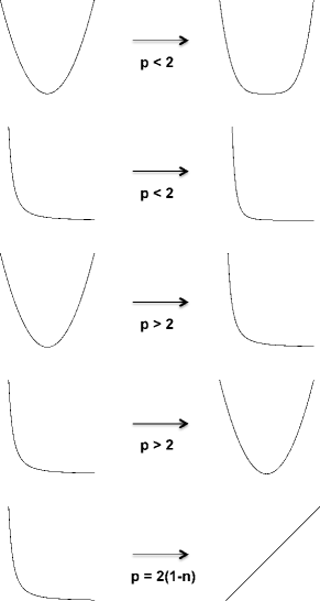
Figure 1: The field transformation to give a canonical kinetic term from one with a pole of order $p$ also transforms the potential. Depending on the value of $p$ this can take monomials and inverse power laws into each other, including linear potentials.

One case of particular interest is $p=4$. This maps a power law index to its negative, i.e.  $\sigma^{n}\to\phi^{-n}$. For an exponential potential $V\sim e^{-\lambda\sigma}$ becomes $V\sim e^{-\lambda\sqrt{k}/\phi}$, again mapping a classic dark energy freezer potential to a well known thawer.

Another case of note is $p\gg 1$. Not only will this convert a thawer to a freezer (since $p>2$) but it will take any monomial with index $m$ and bring it to an inverse power law potential with (negative) index $n\ll 1$. The inverse power law characteristic gives the usual early time attractor dynamics, but the index $n\ll 1$ provides $w_{\rm early}=(-2+nw_{b})/(2+n)\approx-1+n(1+w_{b})/2$, where $w_{b}$ is the background equation of state (e.g. $w_{b}=0$ during the matter dominated era. Thus $p\gg 1$ generates close to cosmological constant like dynamics for any intrinsic monomial potential. Effectively, $p\gg 1$ freezes the dynamics of $\sigma$. This is not dissimilar to screening mechanisms in modified gravity where Vainshtein screening (or k-mouflage) works by decoupling the field through a large kinetic term screen1 ; screen2 ; screen3 .

III Numerical Dynamics

To explore which theories, in terms of pole order and original form of potential, can usefully serve as dark energy, that is be observationally viable in the sense of having $w\approx-1$ at recent times (we will specifically use it in the sense that $w(z)<-0.9$), we consider some standard particle physics potentials and numerically solve the equations of motion of the transformed field.

III.1 Quadratic $\to$ Inverse Power Law

Starting with a quadratic potential, i.e. $V=(1/2)m^{2}\sigma^{2}$, which gives a thawing field, we choose $p>2$. If $p<2$ then the transformed potential will also be a monomial, and a steeper one, making it a less desirable dark energy model. For $p>2$ we will have an inverse power law canonicalized potential, which has the nice feature of an attractor behavior at early times during radiation and matter domination.

However, inverse power law potentials $V\sim\phi^{-\alpha}$ have difficulty attaining $w\approx-1$ by the present, so they are not viable unless the power law index $\alpha\ll 1$ (see, e.g., ratra ). We show the numerically obtained equation of state behavior $w(z)$ in Fig. 2. For $\alpha\lesssim 0.2$ the dark energy evolution is roughly acceptable observationally. Note that it is a freezing model, with a high redshift constant $w$ as discussed in the previous section (with $w\to-0.909$, $-0.952$ for $\alpha=0.2$, 0.1) but approaching $w=-1$ as the universe evolves.

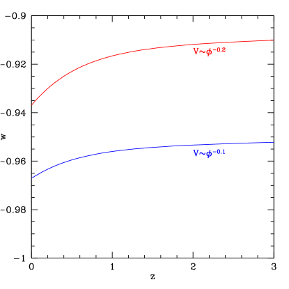
Figure 2: The transformed inverse power law potential is observationally viable for power law index $\alpha=-2n/(2-p)\lesssim 0.2$, with the dark energy equation of state parameter $w(z)<-0.9$.

Freezing fields were studied in detail in 1701.01445 . In particular, for models not too far from $w=-1$ one can compare them to the constant $w$ dark energy defined by the calibration relation $w_{\rm const}=w(a_{\star}\approx 0.85)$. Figure 3 demonstrates that indeed the distance observables in the inverse power law model and its partner constant $w$ agree at the 0.06% level. Note that the field runs to the present over a subPlanckian excursion, $\Delta\phi<M_{P}$.

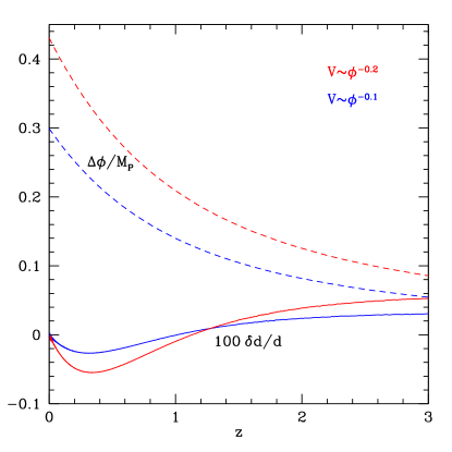
Figure 3: The dark energy behavior from Fig. 2 gives an expansion history similar to constant $w$ models, here $w=-0.963$ and $w=-0.929$ for $\alpha=0.1$, 0.2 (dark blue and light red curves) respectively. The fractional distance deviation from the corresponding constant $w$ model is shown (solid curves) in percent, i.e. the maximum deviation is 0.06%. The field excursion $\Delta\phi$ is subPlanckian (dashed curves).

In pole dark energy one does not have to set the potential to have a shallow inverse power law index. The transformed potential $V\sim\phi^{-0.2}$ can be obtained from a quadratic potential $n=2$ with $p=22$, or a linear potential $n=1$ with $p=12$, or a monodromy potential $n=2/3$ with $p=8.67$.

III.2 Dilation $\to$ Inverse Exponential

Another common particle physics potential is the exponential potential, $V\sim e^{-\beta\sigma}$, such as from dilaton fields. This gives a freezing field, and indeed in the canonical case would trace the background energy density component evolution at early times. When we use this in a Lagrangian with a kinetic pole with $p=4$, we obtain $V\sim e^{-\beta\sqrt{k}/\phi}\equiv e^{-r/\phi}$. Such a potential gives thawing dark energy. The potential is shown in Fig. 4 for three values of $r=\beta\sqrt{k}$.

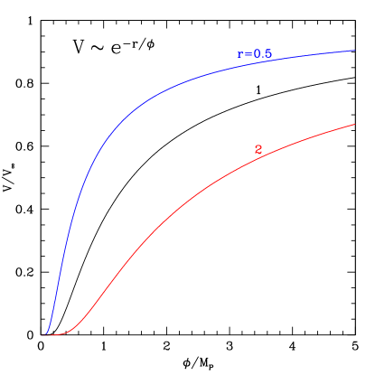
Figure 4: The transformed inverse exponential potential $V\sim e^{-r/\phi}$ has a zero minimum and a plateau, like $\alpha$-attractors, but a weaker one. Nevertheless the field can stay frozen until nearly the present if it does not start too close to the minimum.

Thawing fields were studied in detail in 1501.01634 . In particular, for models not too far from $w=-1$, the field excursion to the present follows

$$\Delta\phi/M_{P}\approx 0.7\sqrt{1+w_{0}}\ .$$ (8)

We verify numerically that holds here. The potential is plateau-like at large $\phi$ (with $\phi=\infty$ corresponding to the pole at $\sigma=0$), but not as flat as an $\alpha$-attractor. Note that near the minimum ($\phi=0$, corresponding to $\sigma=\infty$, so the field cannot roll through zero) the potential is very flat, exponentially so, more than a monomial.

Figure 5 shows the evolution $w(z)$. This can be observationally viable for parameters of order unity. Since the dark energy is a thawing model, it is sensitive to the initial field value $\phi_{i}$ at high redshift (the value $\phi_{i}$ is insensitive to the exact redshift used since the field is frozen until dark energy density becomes appreciable, e.g. $\Delta\phi/M_{P}<0.01$ until $\Omega_{\phi}\approx 0.1$). The steepness of the potential $\lambda=-(1/V)dV/d\phi=-r/\phi^{2}$ helps determine how quickly the field thaws, and we find that the condition $\phi_{i}\gtrsim\sqrt{2r}$ (i.e. $|\lambda_{i}|\lesssim 1/2$) gives observational viability.

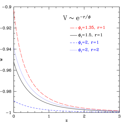
Figure 5: The transformed inverse exponential potential $V\sim e^{-r/\phi}$ gives thawing dark energy, whose equation of state parameter today depends on the coefficient $r$ and the initial field value $\phi_{i}$. It is observationally viable if $\phi_{i}\gtrsim\sqrt{2r}$.

III.3 Poles with $p=2$, and Superexponential

We briefly return to the usual case of kinetic poles with $p=2$, as generally used for inflation. If we use a potential with a pole as well, such as an inverse power law $V\sim\sigma^{-n}$, then this is not covered by the usual Maclaurin expansion $V\approx V_{0}-c\sigma$. However, by Eq. (6) this gives an exponential for the canonicalized potential, $V\sim e^{\mp\phi n/\sqrt{k}}$. Such a potential will not give a satisfactory late time acceleration, unless the field initial conditions are fine tuned to a thawing state (small kinetic energy) rather than the standard scaling solution. Note that like the $p<2$ case, the freezer inverse power law transforms to a freezer potential.

A monomial potential, e.g. $V\sim\sigma^{2}$, is the well known $\alpha$-attractor case (specifically the T model).

Instead we will use a dilaton potential, $V\sim e^{-\beta\sigma}$, which gives rise to a superexponential behavior

$$V\sim e^{-\beta e^{-\phi/\sqrt{k}}}\ .$$ (9)

Near the pole $\sigma=0$ ($\phi=\infty$) one can write this in the usual form

$$V\sim 1-c\sigma\quad\longrightarrow\quad V\sim 1-\beta\,e^{-\phi/\sqrt{k}}\ ,$$ (10)

looking like an $\alpha$-attractor. However, away from the pole one can see the full transformed potential, and in fact the exponential of an exponential imbues it with a flatter plateau than a conventional $\alpha$-attractor, giving an enhanced “basin of attraction” for field initial conditions to yield $w\approx-1$ today.

We plot the transformed potential in Fig. 6. Although $\sigma$ is bounded by $[0,\infty]$, here $\phi$ can range over $[-\infty,\infty]$, with $\sigma=\infty$ corresponding to $\phi=\infty$ (the potential plateau) and $\sigma=0$ corresponding to $\phi=-\infty$ (the potential minimum at zero energy), while $\sigma=1$ gives $\phi=0$.

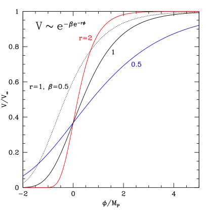
Figure 6: The transformed superexponential potential $V\sim e^{-\beta\,e^{-r\phi}}$ has a zero minimum (at $\phi\ll-1/r$) and a plateau, like $\alpha$-attractors, but an enhanced one. Potentials are plotted vs $\phi$ for various values of $r$, with $\beta=1$ unless otherwise labeled. Increasing $r$ or decreasing $\beta$ enhances the plateau.

Note that increasing $r=1/\sqrt{k}$ or decreasing $\beta$ strengthens the plateau and the attraction to $w\approx-1$. Figure 7 shows the dark energy equation of state evolution. Even initial field values as low as $\phi_{i}/M_{P}=0.37$ (for the $r=1$, $\beta=1$ case), can give observationally viable dark energy behavior – a much smaller value than for most $\alpha$-attractors (for example the Starobinsky model requires $\phi_{i}/M_{P}\gtrsim 1.5$, and an ordinary nonattractor like a quadratic potential requires $\phi_{i}/M_{P}\gtrsim 2.5$, as seen in Fig. 2 of alfde ). One clearly sees that increasing $r$ or decreasing $\beta$ keeps $w(z)$ closer to $-1$. Since this is a thawing field, it again follows the field excursion amplitude given by Eq. (8), and so is subPlanckian. (For notational convenience we will sometimes set $M_{P}=1$.)

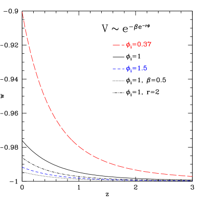
Figure 7: The transformed superexponential potential gives thawing dark energy, whose equation of state parameter today depends on the coefficients $\beta$ and $r$ and the initial field value $\phi_{i}$. It is observationally viable for much lower $\phi_{i}$ than a conventional $\alpha$-attractor. The dark energy equation of state evolution $w(z)$ is plotted for various $\phi_{i}$, with $r=1$, $\beta=1$ unless otherwise labeled. The enhanced potential plateau from increasing $r$ or decreasing $\beta$ leads to a less thawed $w(z)$, one remaining closer to $-1$.

IV Can Poles be Stilts over the Swamp?

Scalar field potentials frequently used for dark energy models can have difficulty being consistent with string theory, in terms of such conditions as swampland criteria 1610.01533 ; 1806.08362 . These conjecture that there is a distance limit $\Delta\phi/M_{P}\lesssim{\mathcal{O}}(1)$ and a steepness criterion $|\nabla V|/V\gtrsim{\mathcal{O}}(1)$.

These conditions impose severe constraints on the types of potentials usually favored for inflation or dark energy. However, we can ask whether the use of poles in the kinetic term can relax the requirements on the potential. This has been mentioned for inflation in terms of noncanonical kinetic terms and the distance criterion in 1807.05445 and for both criteria within multifield inflation in 1807.04390 . In fact, in the latter the field space metric gives an effective noncanonical kinetic term. For inflation, changing the kinetic term can give rise to a tension between satisfying swampland criteria and nongaussianity constraints 1806.09718 .

Dark energy does not have observational nongaussianity limits so it seems worthwhile to explore whether the noncanonical kinetic term used here can ease swampland constraints. In effect, does the pole enable the field to go over the swampland? The answer in a formal sense is no, but in a practical sense is possibly.

For the first criterion, we have already discussed that the field excursions for the models considered, in the observationally viable part of parameter space, follow Eq. (8) for the thawing fields, giving $\Delta\phi/M_{P}<1$. The freezing model of Sec. III.1 also obeyed that limit, as shown in Fig. 3. Of course in the future the field will travel further, but the condition holds in the observable region, the past.

Regarding the steepness criterion, this can also be satisfied under certain conditions. For a noncanonical kinetic term $K(\sigma)(\partial\sigma)^{2}/2$, this takes the form 1806.08362 ; 1807.04390

$$\frac{|\nabla V|}{V}=\frac{1}{\sqrt{K}}\,\frac{|dV/d\sigma|}{V}=\sqrt{\frac{\sigma^{p}}{k}}\,\frac{|dV/d\sigma|}{V}\ .$$ (11)

Indeed, this works out the same as first canonicalizing the field and then simply using $|dV/d\phi|/V$. Nevertheless, our canonicalized potentials are unusual enough that it is worth calculating.

For our first model, a monomial canonicalizing to an inverse power law potential, we have

$$V\sim\sigma^{n}\quad;\quad\frac{|\nabla V|}{V}=\frac{|n|}{\sqrt{k}}\,\sigma^{(p-2)/2}=\frac{2|n|}{|2-p|}\frac{1}{\phi}\ .$$ (12)

Since $p>2$ we need $\sigma\gtrsim 1$ or $\phi\lesssim 1$. At early times $\phi$ can indeed start small and we see we get viable dark energy for subPlanckian excursions so it is possible that the steepness is of order unity, possibly satisfying the steepness criterion.

For the second model, transforming from an exponential to an inverse exponential potential, we have

$$V\sim e^{-\beta\sigma}\quad;\quad\frac{|\nabla V|}{V}=\beta\sqrt{\frac{\sigma^{p}}{k}}\to\frac{\beta\sqrt{k}}{\phi^{2}}\ ,$$ (13)

for our value $p=4$. We can satisfy the criterion for large $r=\beta\sqrt{k}$, but this is observationally unviable since it drives $w$ far from $-1$. Again we want $\sigma\gtrsim 1$ or $\phi\lesssim 1$. As we see in Fig. 5, this makes it more difficult to achieve viable $w(z)$, and this model is not as satisfactory in avoiding the swampland.

For the third model, an exponential canonicalizing to a superexponential, the same condition on $\sigma$ holds,

$$V\sim e^{-\beta\sigma}\quad;\quad\frac{|\nabla V|}{V}=\beta\sqrt{\frac{\sigma^{p}}{k}}\to\frac{\beta}{\sqrt{k}}\,e^{-\phi/\sqrt{k}}\ ,$$ (14)

although the condition is different in terms of $\phi$ (here with $p=2$). Again we would like $\beta$ large, but this is observationally unviable, or $k$ small (i.e. $r$ large), which is ok, but we must make sure that $\phi/\sqrt{k}$ is not large. Fig. 7 demonstrates that these conditions give viable $w(z)$ (as long as $\phi$ isn’t too small, well off the plateau toward the minimum), and so we can potentially achieve $|\nabla V|/V\sim 1$.

Thus at least some of these pole dark energy models seem to have an acceptable range in which they could satisfy both swampland criteria and observational viability in the form of $w(z)<-0.9$ for all redshifts to the present.

V Conclusions and Further Thoughts

Noncanonical kinetic terms can arise from a wide variety of physics, from Dirac-Born-Infeld to higher dimension to coupled models. They add a degree of freedom to quintessence, allowing a dark energy sound speed lower than the speed of light and dynamics in a distinct region of phase space, give nongaussianity in inflation, and enable a type of screening in modified gravity theories. Poles in the kinetic term can arise from several physics mechanisms, and be tied to underlying geometric considerations in string theory. Here we explored the impact of kinetic poles on dark energy and cosmic acceleration in the recent universe.

The transformation from the noncanonical kinetic term into the canonical term, which in $\alpha$-attractor models leads to an extended plateau suitable for inflation (or dark energy), can also turn freezing dark energy into thawing dark energy, and vice versa. We study different order poles and their effect on standard potentials, demonstrating that they can deliver viable dark energy models. In many cases the evolution can approach $w\approx-1$ more easily than in the standard canonical case.

Three example models we study are an inverse power law potential with very small index, generated from a standard quadratic potential (so a thawer transformed to a freezer), an inverse exponential generated from a dilaton field (a freezer transformed to a thawer), and a superexponential coming from a dilaton field. This last model shows an enhanced plateau, flatter than an $\alpha$-attractor, and superattraction in terms of a significantly expanded basin of attraction toward $w\approx-1$ relative to monomials and even $\alpha$-attractors. We also discuss how a high order pole $p\gg 1$ enables cosmological constant like behavior independent of potential, acting in a manner somewhat analogous to Vainshtein screening in modified gravity.

We numerically test all these models for evolution that is observationally viable, in the specific sense that $w(z)<-0.9$. Moreover, all the models exhibit a subPlanckian field excursion (up to the present).

Finally, we consider a more speculative question of whether pole dark energy can avoid swampland criteria difficulties. We have already seen that it satisfies the distance criterion. We demonstrate that indeed the pole models can potentially obey the steepness criterion, yet be observationally viable dark energy with $w\approx-1$. Whether this opens fruitful avenues for dark energy within string theory is left for future work.

The poles in the noncanonical theories lead to interesting new dark energy models such as the superexponential one that exhibits superattraction in the sense of a significantly expanded set of field initial conditions that give rise to observationally viable evolution, and new methods of attaining interesting old dark energy models like a very shallow inverse power law attractor model. Thus pole dark energy appears worthy of future investigation.

References

- (1) R. Kallosh, A. Linde, Universality Class in Conformal Inflation, JCAP 1307, 002 (2013) [arXiv:1306.5220]
- (2) R. Kallosh, A.Linde, D. Roest, Superconformal Inflationary -Attractors, JHEP 1311, 198 (2013) [arXiv:1311.0472]
- (3) M. Galante, R. Kallosh, A. Linde, D. Roest, The Unity of Cosmological Attractors, Phys. Rev. Lett. 114, 141302 (2015) [arXiv:1412.3797]
- (4) J.J.M. Carrasco, R. Kallosh, A. Linde, D. Roest, Hyperbolic geometry of cosmological attractors, Phys. Rev. D 92, 041301 (2015) [arXiv:1504.05557]
- (5) R. Kallosh, A. Linde, CMB Targets after Planck, arXiv:1909.04687
- (6) C. Armendariz-Picon, V. Mukhanov, P. Steinhardt, Dynamical Solution to the Problem of a Small Cosmological Constant and Late-Time Cosmic Acceleration, Phys. Rev. Lett. 85, 4438 (2000) [arXiv:astro-ph/0004134]
- (7) T. Chiba, T. Okabe, M. Yamaguchi, Kinetically Driven Quintessence, Phys. Rev. D 62, 023511 (2000) [arXiv:astro-ph/9912463]
- (8) B.J. Broy, M. Galante, D. Roest, A. Westphal, Pole Inflation – Shift Symmetry and Universal Corrections, JHEP 12, 149 (2015) [arXiv:1507.02277]
- (9) T. Terada, Generalized Pole Inflation: Hilltop, Natural, and Chaotic Inflationary Attractors, Phys. Lett. B 760, 674 (2016) [arXiv:1602.07867]
- (10) E.V. Linder, Dark Energy from -Attractors, Phys. Rev. D 91, 123012 (2015) [arXiv:1505.00815]
- (11) Y. Akrami, R. Kallosh, A. Linde, V. Vardanyan, Dark energy, -attractors, and large-scale structure surveys, JCAP 1806, 041 (2018) [arXiv:1712.09693]
- (12) R.R. Caldwell, E.V. Linder, The Limits of Quintessence, Phys. Rev. Lett. 95, 141301 (2005) [arXiv:astro-ph/0505494]
- (13) T. Baker et al., The Novel Probes Project – Tests of Gravity on Astrophysical Scales, arXiv:1908.03430
- (14) P.G. Ferreira, Cosmological Tests of Gravity, Ann. Rev. Astron. Astroph. 57, 335 (2019) [arXiv:1902.10503]
- (15) M. Ishak, Testing General Relativity in Cosmology, Living Rev. Relativ. 22, 1 (2019) [arXiv:1806.10122]
- (16) J. Ooba, B. Ratra, N. Sugiyama, Planck 2015 constraints on spatially-flat dynamical dark energy models, Astrophys. Space Sci. 364, 176 (2019) [arXiv:1802.05571]
- (17) E.V. Linder, is Coming: Parametrizing Freezing Fields, Astropart. Phys. 91, 11 (2017) [arXiv:1701.01445]
- (18) E.V. Linder, Quintessence’s Last Stand?, Phys. Rev. D 91, 063006 (2015) [arXiv:1501.01634]
- (19) H. Ooguri, C. Vafa, Non-supersymmetric AdS and the Swampland, arXiv:1610.01533
- (20) G. Obied, H. Ooguri, L, Spodyneiko, C. Vafa, De Sitter Space and the Swampland, arXiv:1806.08362
- (21) A. Kehagias, A. Riotto, A note on Inflation and the Swampland, Fort. Phys. 66, 1800052 (2018) [arXiv:1807.05445]
- (22) A. Achúcarro, G.A. Palma, The string swampland constraints require multi-field inflation, JCAP 1902, 041 (2019) [arXiv:1807.04390]
- (23) P.Agarwal, G. Obied, P.J. Steinhardt, C. Vafa, On the Cosmological Implications of the String Swampland, Phys. Lett. B 784, 271 (2018) [arXiv:1806.09718]