Two-dimensional Inflow-outflow Solution of Supercritical Accretion Flow

Abstract

We present the two-dimensional inflow-outflow solutions of radiation hydrodynamic (RHD) equations of supercritical accretion flows. Compared with prior studies, we include all components of the viscous stress tensor. We assume steady state flow and use self-similar solutions in the radial direction to solve the equations in $r-\theta$ domain of the spherical coordinates. The set of differential equations have been integrated from the rotation axis to the equatorial plane. We find that the self-similarity assumption requires that the radial profile of density is described by $\rho(r)\propto r^{-0.5}$. Correspondingly, the radial profile of the mass inflow rate decreases with decreasing radii as $\dot{M}_{\mathrm{in}}\propto r$. Inflow-outflow structure has been found in our solution. In the region $\theta>65^{\circ}$ there exist inflow while above that flow moves outward and outflow could launch. The driving forces of the outflow are analyzed and found that the radiation force is dominant and push the gas particles outwards with poloidal velocity $\sim 0.25c$. The properties of outflow are also studied. The results show that the mass flux weighted angular momentum of the inflow is lower than that of outflow, thus the angular momentum of the flow can be transported by the outflow. We also analyze the convective stability of the supercritical disk and find that in the absence of the magnetic field, the flow is convectively unstable. Our analytical results are fully consistent with the previous numerical simulations of the supercritical accretion flow.

1 Introduction

Accretion of gas through a disc onto a black hole is associated with many active phenomena in our universe such as active galactic nuclei (AGNs), X-ray binaries (XRBs), and extra galactic jets. Based on temperature, black hole accretion discs can be divided into two distinct classes: hot and cold (see Yuan & Narayan 2014 for review). Hot accretion flow consists of optically thin, and geometrically thick disc with very low mass accretion rate (e.g. Narayan & Yi 1994, 1995; Blandford & Begelman 1999, 2004; Yuan et al. 2012a, b; Mosallanezhad et al. 2014, 2016; Zeraatgari & Abbassi 2015; Zeraatgari et al. 2018). While, in cold accretion flow, the disc is optically thick with relatively high mass accretion rate.

In terms of cold accretion flow, standard thin disc model is the first authentic model of black hole accretion disc (Shakura & Sunyaev 1973; Novikov & Thorne 1973, Lynden-Bell & Pringle 1974; Pringle 1981). In this model the heat generated by the viscosity locally radiates away from the disc. Consequently, the disc temperature becomes far below the virial temperature, i.e., $10^{4}-10^{7}\,K$. The criterion for mass accretion rate is the Eddington rate defined as $\dot{M}_{\mathrm{Edd}}=L_{\mathrm{Edd}}/(\eta c^{2})$, where $L_{\mathrm{Edd}}$ is the Eddington luminosity, $\eta$ is the radiative efficiency, and $c$ is the speed of light. The thin disc model can successfully be applied to many black hole systems when their mass accretion rate are slightly low, $\dot{M}\lesssim\dot{M}_{\mathrm{Edd}}$ (e.g., Pringle 1981; Frank et al. 2002; Kato et al. 2008; Abramowicz & Fragile 2013; Blaes 2014; Koratkar & Blaes 1999; Remillard & McClintock 2006; McClintock et al. 2014).

When the accretion rate is above the Eddington limit, advection becomes important, and the accretion flow can be described by the Super-Eddington (or supercritical) flow. In this case, the radiative diffusion timescale, $t_{\mathrm{diff}}$, can exceed the timescale for accretion, $t_{\mathrm{acc}}$, as a consequence of the high mass accretion rate. Thus, the diffused photons cannot escape from the disc and accrete onto the black hole with gas particles. Note that in some 3D RMHD simulation of super-Eddington accretion (e.g., Jiang et al. 2014), they found that radiative transfer in the vertical direction is important thus photon trapping is not as strong as people previously thought.

The HD and MHD numerical simulations of hot accretion flow have found that mass inflow rate decreases inward ( e.g., Stone et al. 1999; Yuan et al. 2012b). In this regards, various analytical works proposed to explain this result such as adiabatic inflow-outflow solution (ADIOS, Blandford & Begelman 1999, 2004, Begelman 2012) and convection dominated accretion flow (CDAF, Narayan et al. 2000). Based on ADIOS model, mass loss in the outflow is the reason for the inward decrease of the mass accretion rate. Therefore, due to the presence of outflow the mass accretion rate is not a constant with radius and decreases towards the black hole. CDAF model also presented to explain the simulations is assumed to be convectively unstable. However, recent numerical simulations have shown that MHD accretion flows are convectively stable (Narayan et al. 2012, Yuan et al. 2012a).

In the case of the supercritical accretion flow, the outflow/wind is unavoidable. Since the accretion luminosity exceeds Eddington limit, the radiation force becomes much more greater than the gravity. Subsequently, at high latitudes, the gas particles can be accelerated by the radiation pressure and blown out from the system as multi-dimensional effects like jet/wind. Some good candidates for supercritical accretion flows are ultra-luminous X-ray sources (ULXs), ultra-soft X-ray sources (ULSs), narrow-line Seyfert 1 galaxies (NLS1s), bright micro-quasars (see, e.g., Wang & Zhou 1999; Boller 2000; Mineshige et al. 2000; Makishima et al. 2000; Miller et al. 2004, Done et al. 2007; Vierdayanti et al. 2010; Fürst et al. 2016; Israel et al. 2017a, b; Kaaret et al. 2017; Kosec et al. 2018).

Several multi-dimensional/time-dependent radiation hydrodynamic (RHD), radiation magnetohydrodynamic (RMHD) and general relativistic-radiation magnetohydrodynamic (GR-RMHD) simulations have been performed to reveal the physical properties of the supercritical flows (Eggum et al. 1987, 1988; Okuda 2002; Okuda et al. 2005; Ohsuga et al. 2005; Ohsuga & Mineshige 2007; Ohsuga et al. 2009; Kawashima et al. 2009, 2012; Ohsuga & Mineshige 2011; Yang et al. 2014; Jiang et al. 2014; Sadowski et al. 2014, 2015; McKinney et al. 2014; Fragile et al. 2014; Takahashi et al. 2016; Kitaki et al. 2017; Kitaki et al. 2018). The first one-dimensional analytical studies on super-Eddington accretion flow, i.e., the slim disc model have focused on the radial structure of the flow (Begelman & Meier 1982; Abramowicz et al. 1988; Wang & Zhou 1999; Watarai & Fukue 1999; Mineshige et al. 2000; Watarai et al. 2000, 2001; Watarai 2006; Fukue 2004; Gu & Lu 2007). They used cylindrical coordinates ($R,\phi,z$) and adopted $H=c_{\mathrm{s}}/\Omega_{\mathrm{K}}$ for the disc height, where $c_{\mathrm{s}}$ and $\Omega_{\mathrm{K}}$ are the sound speed and the Keplerian velocity, respectively. In the mentioned relation, based on hydrostatic equilibrium in the vertical direction, the disc height was considered constant. Although this approximation might be true for standard thin disc model, it is obviously inaccurate for supercritical disc where the disc is geometrically thick due to the high mass accretion rate. However, Zeraatgari et al. 2016 solved the $1.5-$dimensional inflow-outflow equations of supercritical accretion flow by assuming a power-law function for mass accretion rate, $\dot{M}\propto r^{s}$. They found that $s=1$ due to the inclusion of the radiative cooling. Ohsuga et al. 2005 is one of the pioneer numerical simulation works which considered a relatively small angular momentum for the flow and obtained quasi-steady state solutions. They found a small inflow region near the equatorial plane and very wide angle outflow region above the disc.

To reveal the complex two-dimensional structure and understanding the physical properties of the supercritical accretion flow, Gu 2012 adopted spherical polar coordinates and considered only $T_{r\phi}$ component of the stress tensor to mimic the angular momentum transfer by the magneto-rotational instability (MRI, Balbus & Hawley 1998). He assumed that the radiation pressure is much more stronger than the gas pressure, i.e., $p_{\mathrm{gas}}/p_{\mathrm{rad}}\ll 1$. He further assumed $v_{\theta}=0$ which is obviously incorrect for the extremely high mass accretion rate. By making use of the radial self-similar solutions, he showed that the polytropic relation adopted in previous analytical works was not suitable. He found that even for marginally sub-Eddington accretion flow the energy advection was significant and the accretion disc was convectively stable.

In the present study, we revisit the inflow-outflow structure of the supercritical accretion flow by means of radial self-similar solution. The main aim of this study is to relax the assumption of $v_{\theta}=0$ compared with Gu 2012 and consider very high mass accretion rate (see figure 1 of Gu 2012 for more details). To do so, we adopt spherical coordinations and consider all components of the velocity, i.e., ($v_{r},v_{\theta},v_{\phi}$) and also all components of the viscous stress tensor. We integrate the set of coupled RHD equations in the whole vertical angle, from rotational axis to the equatorial plane. Therefore, compare to the previous analytical works, we can clearly show two dimensional structure of the supercritical disc and address its physical properties when the disc is in the steady state.

The remainder of the manuscript is organized as follows. The basic equations and assumptions are described in section 2. The self-similar solutions and boundary conditions are given in Section 3. In Section 4, the numerical results are presented with detailed explanations. Finally, the summary and discussion are provided in Section 5.

2 BASIC EQUATIONS AND ASSUMPTIONS

In this section, we describe the two-dimensional RHD equations of accretion flow around a non-rotating black hole in spherical coordinates ($r,\theta,\phi$). We neglect the self-gravity of the accretion disc. To avoid the relativistic effects, the Newtonian potential, $\psi=-(GM)/r$, is considered, where $G$ is the gravitational constant and $M$ is the black hole mass. The basic RHD equations of the accretion flow are written as follows,

$$\frac{\partial\rho}{\partial t}+\bm{\nabla}\cdot\left(\rho\bm{v}\right)=0,$$ (1)

$$\rho\left[\frac{\partial\bm{v}}{\partial t}+\left(\bm{v}\cdot\bm{\nabla}\right)\bm{v}\right]=-\rho\bm{\nabla}\psi-\bm{\nabla}p_{\mathrm{gas}}+\bm{\nabla}\cdot\bm{\sigma}+\frac{\chi}{c}\,\bm{F},$$ (2)

$$\frac{\partial e}{\partial t}+\bm{\nabla}\cdot\left(e\bm{v}\right)=-p_{\mathrm{gas}}\bm{\nabla}\cdot\bm{v}-4\pi\kappa B+c\kappa E+\Phi_{\mathrm{vis}},$$ (3)

$$\frac{\partial E}{\partial t}+\bm{\nabla}\cdot\left(E\bm{v}\right)=-\bm{\nabla}\cdot\bm{F}-\bm{\nabla v:P}+4\pi\kappa B-c\kappa E.$$ (4)

In the above equations, $\rho$ is the density, $\bm{v}\left[=(v_{r},v_{\theta},v_{\phi})\right]$ is the velocity, $p_{\mathrm{gas}}$ is the gas pressure, $\bm{\sigma}$ is the viscous stress tensor, $\chi$ is the total opacity, $\bm{F}$ is the radiation flux, $e$ is the internal energy density of the gas, $E$ is the radiation energy density, $\bm{P}$ is the radiation pressure tensor, $\kappa$ is the absorption opacity, $B$ is the blackbody intensity, and $\Phi_{\mathrm{vis}}$ is the viscous dissipative function. The viscous stress tensor can be described as,

$$\sigma_{ij}=\mu\left[\left(\frac{\partial v_{j}}{\partial x_{i}}+\frac{\partial v_{i}}{\partial x_{j}}\right)-\frac{2}{3}\left(\bm{\nabla}\cdot\bm{v}\right)\right]$$ (5)

where $\mu(\equiv\nu\rho)$ is the dynamical viscosity coefficient which determines the magnitude of the stress and $\nu$ is called the kinematic viscosity coefficient. We note that the bulk viscosity is neglected in this study. The dynamical viscosity coefficient is calculated with the usual $\alpha$ prescription of the viscosity (Shakura & Sunyaev 1973),

$$\mu=\alpha\frac{p_{\mathrm{gas}}+\lambda E}{\Omega_{K}},$$ (6)

where $\alpha$ is the viscosity parameter, $\lambda$ is the flux limiter, and $\Omega_{K}\equiv(GM/r^{3})^{1/2}$ is the Keplerian angular momentum. To calculate the radiation flux, $\bm{F}$, we apply the flux-limited diffusion (FLD) approximation (Levermore & Pomraning 1981) as,

$$\bm{F}=-\frac{\lambda c}{\chi}\,\mathbf{\nabla}E,$$ (7)

where $\lambda$ is flux limiter. To avoid the complexity, the absorption opacity including both free-free absorption, $\kappa_{\mathrm{ff}}$, and bound-free absorption, $\kappa_{\mathrm{bf}}$, are neglected in the present study. The total opacity is then $\chi=\rho\kappa_{\mathrm{es}}$, where $\kappa_{\mathrm{es}}$ is the electron scattering opacity. The radiation pressure tensor is calculated in terms of energy density of the radiation as,

$$\mathbf{P}=\bm{f}E,$$ (8)

where $\bm{f}$ is the Eddington tensor. In this study we focus on optically thick region, where $\lambda=1/3$ and $\bm{f}=\bm{I}/3$ (Kato et al. 2008). Thus, the Eddington approximation yields to,

$$\bm{P}_{ij}=\begin{cases}p_{\mathrm{rad}}=E/3\quad\quad\quad&\text{if}\quad i=j,\\ 0&\text{if}\quad i\neq j.\end{cases}$$ (9)

By combining equation(3) and equation(4), the total energy equation including gas and radiation can be rewritten as,

$$\frac{\partial\left(e+E\right)}{\partial t}+\bm{\nabla}\cdot\left[\left(e+E\right)\bm{v}\right]=-(p_{\mathrm{gas}}+p_{\mathrm{rad}})\bm{\nabla}\cdot\bm{v}\\ -\bm{\nabla}\cdot\bm{F}+\Phi_{\mathrm{vis}},$$ (10)

where $p_{\mathrm{rad}}$ is radiation pressure and based on our assumption it is much more stronger than the gas pressure, i.e., $p_{\mathrm{gas}}/p_{\mathrm{rad}}\ll 1$. Thus, the gas pressure as well as internal energy density of the gas will be dropped in our equations. We consider steady-state and axisymmetric ($\partial/\partial t=\partial/\partial\phi=0)$ flow to solve equations (1)-(4). The detailed form of partial differential equations (PDEs) are presented in Appendix A, (see equations [A7]-[A13]). We outline our self-similar solutions and boundary conditions in the following section.

3 Self-similar Solutions and Boundary Conditions

Many numerical simulations of accretion flow show that the radial profile of the density can be described as a power law function of $r$ as $\rho(r)\propto r^{-n}$. In terms of hot accretion flow, the global numerical simulations are consistent with the self-similar assumptions away from the boundaries (e.g., Stone et al. 1999; Yuan et al. 2012a, b; Yuan et al. 2015). For the case of super-Eddington accretion flow, recent numerical simulations also show that the radial profile of the density follows a power law form with $n\approx 0.55$ for a wide range of $\alpha$ from $\alpha=0.005$ to $0.1$ (Ohsuga et al. 2005, Yang et al. 2014) . Therefore, in order to solve the equations ([A7]-[A11]), by numerical methods, we adopt self-similar solutions to remove the radial dependence of the variables.

3.1 Self-similar Solutions

By considering a fiducial radial distance, i.e., $r_{0}$, the self-similar solutions can be written as a power-law form of $r/r_{0}$. Thus, the physical variables of the flow can be written by the following radial scaling,

$$v_{r}\left(r,\theta\right)=v_{0}\left(\frac{r}{r_{0}}\right)^{-1/2}v_{r}(\theta),$$ (11)

$$v_{\theta}\left(r,\theta\right)=v_{0}\left(\frac{r}{r_{0}}\right)^{-1/2}v_{\theta}(\theta),$$ (12)

$$v_{\phi}\left(r,\theta\right)=v_{0}\left(\frac{r}{r_{0}}\right)^{-1/2}\Omega(\theta)\sin\theta,$$ (13)

$$\rho\left(r,\theta\right)=\rho_{0}\left(\frac{r}{r_{0}}\right)^{-n}\rho(\theta),$$ (14)

$$p_{\mathrm{rad}}\left(r,\theta\right)=\rho_{0}v_{0}^{2}\left(\frac{r}{r_{0}}\right)^{-n-1}p(\theta),$$ (15)

where $v_{0}=(GM/r_{0})^{1/2}$ and $\rho_{0}$ are considered to be Keplerian velocity and density at $r_{0}$, respectively. By substituting above self-similar solutions into equations [A7]-[A11], the radial dependency will be removed only if $n=1/2$. This is mainly due to the inclusion of the radiative cooling in the energy equation, i.e., $\bm{\nabla}\cdot\bm{F}$. Consequently, the radial profile of the accretion rate can be well described by $\dot{M}\propto r$ which is fully consistent with hyperaccreting ADIOS model of Begelman 2012. This result is again consistent with the radial dependency of the density found in this present study.

Substituting equations (11)-(15) into equations ([A7]-[A11], we can reduce them to ordinary differential equations (ODEs) given in Appendix (B). Equations (B1)-(B5) describe the variations of the five physical quantities, $v_{r}(\theta)$, $v_{\theta}(\theta)$, $v_{\phi}(\theta)$, $\rho(\theta)$, and $p(\theta)$ in the vertical direction.

Figure 1: Angular profile of the physical variables at $r=10r_{s}$. Top-left panel: radial velocity in the unit of light speed, $c$. Dashed line shows the location of $v_{r}=0$ that is about $65^{\circ}$. Top-middle panel: latitudinal velocity in the unit of Keplerian velocity, $v_{0}$. Top-right panel: Angular velocity in the unit of Keplerian angular velocity, $\Omega_{0}$. Bottom-left panel: density in the unit of density of mid-plane at $r_{0}$, i.e., $\rho_{0}$. Bottom-middle panel: radiation pressure in the unit of $\rho_{0}v_{0}^{2}$. Bottom-right panel: Mach numbers.

Figure 2: Two-dimensional distribution of the density (left panel) and the temperature (right panel) based on the self-similar solutions. Both panels overlaid with the poloidal velocity. In the left panel, the poloidal velocity is normalized by $0.1c$ to denote the strength of the outflow while in the right panel, the poloidal velocity is normalized with its absolute value to denote the direction of the vectors.

3.2 Boundary Conditions

Following Narayan & Yi 1995, we assume that all flow variables are even symmetric, continuous, and differentiable at the equatorial plane, $\theta=\pi/2$, and the rotation axis, $\theta=0$. The main difference here compare to the previous works is that we include the latitudinal component of the velocity, $v_{\theta}$, in our equations and consider it to be zero at both the equatorial plane and the rotation axis. Therefore, we apply the following boundary conditions at $\theta=\pi/2$ and $\theta=0$:

$$v_{\theta}=\frac{\mathrm{d}\rho}{\mathrm{d}\theta}=\frac{\mathrm{d}p}{\mathrm{d}\theta}=\frac{\mathrm{d}v_{r}}{\mathrm{d}\theta}=\frac{\mathrm{d}\Omega}{\mathrm{d}\theta}=0$$ (16)

To solve the set of ODEs, (see equations [B1]-[B5] in Appendix B), we need to set fiducial radial distance, $r_{0}$ and the density there, $\rho_{0}$, which are defined in equations (11)-(15), (see the constant term, $\tau^{-1}(c/v_{0})$, in the right-hand side of the equation [B5] as well). Numerical simulations of accretion flow show that the radial velocity increases inward very rapidly because of the strong gravity near the black hole (Ohsuga et al. 2005, Yuan et al. 2012a, b). To avoid shock occurring by supersonic inflow near the central region, which is a source of deviation from the self-similar assumptions, we neglect the region within $10r_{\mathrm{s}}$, where $r_{\mathrm{s}}=2GM/c^{2}$ is the Schwarzschild radius (see e.g., Kawashima et al. 2012, Jiang et al. 2014). Due to the assumption of high mass accretion rate, we expect strong radiation produced at the innermost region interacts with gas particles at the region $r\gtrsim 10r_{\mathrm{s}}$ and strong outflow is driven there. To show the two dimensional inflow-outflow structure of the flow, we consider all components of the velocity including $v_{\theta}$ in our equations. Throughout present study, we set the inner and outer radial range of the domain as $r_{\mathrm{min}}=10r_{\mathrm{s}}$ and $r_{\mathrm{max}}=500r_{\mathrm{s}}$, respectively. Thus, the assumption of Newtonian potential is safely valid in this range. We set $r_{0}=10r_{\mathrm{s}}$ and for the initial density, $\rho_{0}$, we calculate the mass inflow rate at the outer radial boundary. Following numerical simulations of supercritical accretion flow, the dimensionless mass inflow rate defines as (see Ohsuga et al. 2005, Yang et al. 2014)

$$\dot{m}=-\frac{c^{2}}{L_{\mathrm{Edd}}}\int_{0}^{\pi}2\pi r^{2}\rho\,\mathrm{min}\left(v_{r},0\right)\,\sin\theta\,d\theta.$$ (17)

We set $\dot{m}=1300$ at the outer radial boundary, i.e., $r_{\mathrm{max}}=500r_{\mathrm{s}}$ throughout this paper. Based on self-similar solutions adopted here, the mass inflow rate in this study is not radially constant and decreases inward as $\dot{m}\propto r$. We use iteration method to find the value of $\rho_{0}$ by solving equation (17) at the outer radial boundary.

4 Numerical results

We solve the ordinary differential equations [B1]-[B5] by integrating from the equatorial plane ($\theta=\pi/2$) to the rotation axis ($\theta=0$). We adopt the values of $\alpha=0.1$, $M=10M_{\odot}$, and $\kappa_{\mathrm{es}}=0.34$ with reference to the numerical simulations of Ohsuga et al. 2005 and Yang et al. 2014. The main difference here compare to those numerical simulations is that we consider all components of viscous stress tensor. As it is expressed in previous section, the radial range of our calculation is $10r_{\mathrm{s}}\leq r\leq 500r_{\mathrm{s}}$. We implement relaxation method to solve the set of equations along the vertical direction. The grid in $\theta$ direction is divided into 2000 equally spaced points and iteration technique is used to find the value of $\rho_{0}$ with $\dot{m}=1300$ at $r_{\mathrm{max}}$. For this constant mass accretion rate, we obtain $\rho_{0}=2.89\times 10^{-5}\mathrm{gr/cm^{3}}$. We can reasonably treat this value as a boundary condition. The global properties of the solutions we obtain in this way agree well with those presented in numerical simulations of Ohsuga et al. 2005 and Yang et al. 2014. In the following subsections, we explain in details the flow properties based upon our solutions.

4.1 Inflow-outflow structure of the solutions

Figure 1 presents angular profiles of physical quantities at $r=10r_{\mathrm{s}}$. We can see, the density and the radiation pressure decrease rapidly from the equatorial plane to the rotation axis. Since we are interested in studying the case where the radiation pressure is much more stronger than the gas pressure, i.e., $p_{\mathrm{gas}}/p_{\mathrm{rad}}\ll 1$, this pressure represents the total pressure of the flow. As it is shown in the top-left panel of Figure 1, at the region close to the equatorial plane, $\theta>65^{\circ}$, the radial velocity is negative and the gas particles move toward the central black hole. While, in the region, $\theta<65^{\circ}$, the sign of the radial velocity changes and becomes positive. Furthermore, the top-middle panel shows the variation of $v_{\theta}$ along the vertical direction. From this plot, it is seen that $v_{\theta}$ has a negative value in all angles, and is zero at both the equatorial plane and the rotation axis due to the boundary conditions. The minimum value of $v_{\theta}$ is also located around $\theta\sim 43^{\circ}$. Moreover, the bottom-right panel of Figure 1 represents the Mach numbers. We plot this figure to check the existence of the sonic point at the high-latitude region. As we can see, there does not exist any sonic points in this region. The Mach number $|v_{r}|/c_{s}$ decreases from the equatorial plane to about $65^{\circ}$, where the radial velocity is zero. Then, it increases until $\theta=30^{\circ}$ and again decreases rapidly to the rotation axis. This behavior can be explained by the isothermal sound speed, $c_{\mathrm{s}}=p/\rho$. The profile of the density and the total pressure in Figure 1 show that the density decreases rapidly from the equator to the pole while the pressure is almost constant at the range $0<\theta<30^{\circ}$. Therefore, the Mach number declines in this range. Also, $|v_{\theta}|/c_{\mathrm{s}}$ has a maximum value at $\theta=43^{\circ}$ and becomes null at both axes due to the boundary conditions there, i.e, $v_{\theta}=0$. For both lines, the Mach numbers are less than unity which clearly shows that there is no critical point at high latitudes.

In the left panel of Figure 2, we plot two-dimensional distribution of the density overlaid with the stream lines of the flow. The results are shown for $\dot{m}=1300$ and the poloidal velocity is normalized by $0.1c$. It can be seen, the density tends to be larger around mid-plane than that around the polar axis. Moreover, the stream lines are directed toward the black hole at low latitudes with small magnitudes. At high latitudes, they are pointed outward and become outflow. For high accretion rate, as in our present study, the outflow can be driven by the radiation pressure produced at inner radii. This strong radiation interacts with the gas particles and can push them away as high velocity outflow. This figure clearly shows the high velocity field region at high latitudes at $r=10r_{\mathrm{s}}$. As shown in top-left and top-middle panels of figure 1, the poloidal velocity of outflow reaches to about $\sim 0.25c$. These results are fully consistent with the results obtained in Yang et al. 2014 (see Fig. 1) and Ohsuga et al. 2005, where the inflow is presented in low latitude around the equatorial plane of the disc while outflow is presented at high latitude regions.

The two-dimensional profile of the radiation temperature, $T=(E/a)^{1/4}$, is plotted in the right panel of Figure 2, (where, $a=7.5646\times 10^{-15}\,\mathrm{erg}\,\mathrm{cm}^{-3}\,\mathrm{K}^{-4}$ is the radiation constant). The logarithm of the temperature is overlaid with the poloidal velocity normalized with its absolute value denotes the direction of the vectors. With the assumption of $p_{\mathrm{gas}}/p_{\mathrm{rad}}\ll 1$, the gas and the radiation are in equilibrium, so their temperatures are almost equal. Due to the heating of the gas by the viscous dissipation, the temperature is relatively higher in the inner region than that at the outer radii. Therefore, this produced energy can be effectively converted into the radiation energy. This figure somehow represents the distribution of the radiation internal energy density. In addition, at large radii with high latitudes, we can see the temperature is lower than one at low latitudes with the same radii. This is the consequence of the radiative cooling by the outflow.

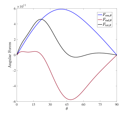
Figure 3: Angular distribution of the radial forces (left panel), and angular forces (right panel) per unit mass at $r=10r_{\mathrm{s}}$. The forces include gravity (black dotted line), centrifugal force (blue solid line), radiation force (red solid line), and their sum (black solid line).

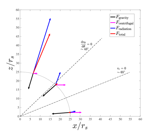
Figure 4: Force analysis at inflow/outflow region to show the driving mechanism of the outflow at $r=25r_{\mathrm{s}}$. The length of the arrows schematically denotes the magnitude of the forces while the direction for the direction of forces. The forces include gravity, centrifugal, radiation, and the sum of them. The dash-dotted line shows the location of $v_{r}=0$, the dashed line represents the location of $\frac{\mathrm{d}v_{\theta}}{\mathrm{d}\theta}=0$, and dotted line shows the radius where the forces calculated.

4.2 Physical properties of the outflow

In this subsection we calculate the physical properties of the outflow based on our self-similar solutions. In the top-right panel of Figure 1 the angular velocity of the accretion flow is plotted. It is seen that the angular velocity increases from the equatorial plane to the rotation axis and becomes almost Keplerian at high latitudes which is consistent with Yuan et al. 2012a numerical simulation results. This indicates that the outflow can transport angular momentum outward from the disc. To check this issue in more detail, we evaluate the mass flux weighted value of the inflow and the outflow quantities as,

$$Q_{\mathrm{in}}(r)=\frac{4\pi r^{2}\int^{\pi/2}_{0}\rho Q\,\mathrm{min}(v_{r},0)\sin\theta d\theta}{4\pi r^{2}\int^{\pi/2}_{0}\rho\,\mathrm{min}(v_{r},0)\sin\theta d\theta},$$ (18)

$$Q_{\mathrm{out}}(r)=\frac{4\pi r^{2}\int^{\pi/2}_{0}\rho Q\,\mathrm{max}(v_{r},0)\sin\theta d\theta}{4\pi r^{2}\int^{\pi/2}_{0}\rho\,\mathrm{max}(v_{r},0)\sin\theta d\theta},$$ (19)

where, $Q$ represents the physical quantities. The mass flux weighted angular momentum of the inflow and the outflow are found as,

$$L_{\mathrm{in}}=0.79\,L_{K},$$ (20)

and

$$L_{\mathrm{out}}=0.89\,L_{K},$$ (21)

where $L_{K}$ is the Keplerian angular momentum. This result clearly shows that the angular momentum of the flow can be transferred by the outflow which is fully consistent with the numerical simulation results of supercritical accretion discs (see Ohsuga et al. 2005 and Yang et al. 2014). We also define the Bernoulli parameter as,

$$Be(r)=\frac{v^{2}}{2}+\frac{\gamma p}{\left(\gamma-1\right)\rho}-\frac{GM}{r},$$ (22)

where, $\gamma=4/3$ is the specific heat ratio. The Bernoulli parameter is the sum of the kinetic energy, the enthalpy, and the gravitational energy of the accreting gas. The mass flux weighted Bernoulli parameter of the outflow is obtained as,

$$Be=2.67\,v_{\!K}^{2}.$$ (23)

The value of the Bernoulli parameter is positive which shows the outflow has enough energy to overcome the gravity of the central back hole and escape to the infinity. The mass flux weighted poloidal velocity of the outflow, i.e., $v_{\mathrm{pol}}^{2}=v_{r}^{2}+v_{\theta}^{2}$, is also calculated as,

$$v_{\mathrm{pol}}=0.44\,v_{\!K}.$$ (24)

Here, we conclude that the radiation driven outflow has enough energy and power to interact with its surrounding, overcome the gravitational potential and escape to the infinity.

4.3 Analysis of forces driving the outflow

In order to understand which force can drive outflow from our system, we plot in Figure 3 the angular distribution of the radial forces (left panel) and the angular forces (right panel) at $r=10r_{\mathrm{s}}$. We can see from the left panel of this figure that the angular profile of the total force has similar behavior with the angular profile of the radial velocity shown in Figure 1. In addition, left panel of Figure 3 shows that within $60^{\circ}<\theta<90^{\circ}$ the radial component of the centrifugal force is greater than the radial component of the radiation force and can effectively counteracts the gravitational force in this range. However, within $0^{\circ}<\theta<60^{\circ}$, the radial component of the centrifugal force decreases rapidly and becomes null at the rotation axis. In contrast, the radial component of the radiation force is the dominant force near the rotation axis and we can see there exists very strong outflow near this axis. Therefore, it can be concluded that the radial radiation force is the dominant force and plays the important role to drive outflow at high latitudes. It is interesting here to compare this result with the case of hot accretion flows (Yuan et al. 2015), in which radiation can be neglected. Although the dominant driving force is different in the two cases, outflow is always present and even their properties are similar.

It is seen from left panel of Figure 3, the angular component of the total force is very small at the region near the equatorial plane, i.e., $50^{\circ}<\theta<90^{\circ}$, which clearly shows that the flows are in the force equilibrium in the inflow region. This is mainly because from this panel we can see that the centrifugal force balances with the radiation force in the vertical direction. The angular distribution of both the radiation force and the centrifugal force become zero at both axes due to the boundary conditions.

To have a better understanding of the magnitude of the forces in different $\theta$ angels and study the driving mechanisms of the outflow, we calculate the forces at different regions. Figure 4 shows the result at $r=25r_{\mathrm{s}}$ in the unit of gravity. We can see from this figure that at the inflow region, $\theta=85^{\circ}$, the dominant force is the gravity so, the flow moves toward the central black hole. In the intermediate region, $\theta=45^{\circ}$, the driving forces are the centrifugal and the radiation forces. As it is seen, the strength of these forces are comparable means both of them can drive outflow in this region, but not so strong. Instead, at very high latitudes, $\theta=15^{\circ}$, the radiation force can efficiently offset the gravity and play a noticeable role in driving the outflow whereas the centrifugal force is negligible and does not have any efficient contribution to the total force. These results are again fully consistent with those found in Yang et al. 2014 and Ohsuga et al. 2005.

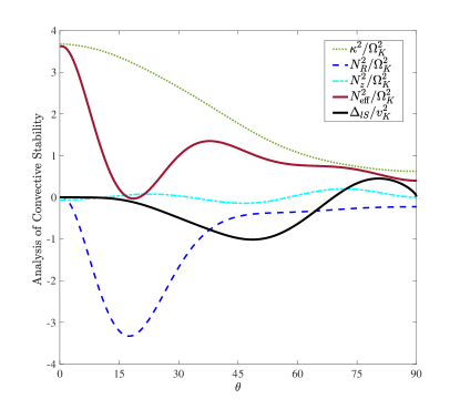
Figure 5: Angular variations of $\kappa^{2}$ ( green dotted line), $N_{R}^{2}$ (blue dashed line), $N_{z}^{2}$ (cyan dash-dotted line), $N^{2}_{\mathrm{eff}}$ (red solid line), and $\Delta_{lS}$ (black solid line). The quantities $\kappa^{2}$, $N_{R}^{2}$ , $N_{z}^{2}$ , and $N^{2}_{\mathrm{eff}}$ are normalized by $\Omega_{K}^{2}$, and $\Delta_{lS}$ is normalized by $v_{\!{K}}^{2}$.

4.4 Convective stability

In term of supercritical accretion flow, due to the large scattering optical depth, the photons produced from innermost part of the disc are trapped and cannot efficiently escape from the disc. Furthermore, the specific entropy is dominated mostly by the radiation photons since the radiation pressure is much more important than the gas pressure here. Several analytical and simulation works have been done to study the convective stability of supercritical accretion flows. For instance, based on the local energy balance, Sadowski et al. 2009 and Sadowski et al. 2011 found that the disc is convectively unstable. However, Gu 2012 used self-similar solutions and concluded that radiation pressure-supported disc is always convectively stable. This discrepancy between these works might be related to the different definition of vertical structure of the disc. In terms of numerical simulation, Yang et al. 2014 studied this issue based on their simulation data for large and small values of viscosity parameter. They found that for large value of viscosity parameter, $\alpha=0.1$, about half of the computational domain was convectively unstable, while for $\alpha=0.005$, the fraction of the unstable region was much less. They concluded that radiation plays an effective role to stabilize the convection and can directly transport energy.

In this subsection, we revisit this problem and analyze the convective stability of supercritical accretion flow, in the absence of magnetic field, based on our self-similar solutions. Thus, we use the well-known Solberg-Høiland criterions in cylindrical coordinates $(R,\phi,z)$ as follows,

$$\frac{1}{R^{3}}\frac{\partial l^{2}}{\partial R}-\frac{1}{C_{P}\rho}\bm{\nabla}P\cdot\bm{\nabla}S>0,$$ (25)

$$-\frac{\partial P}{\partial z}\left(\frac{\partial l^{2}}{\partial R}\frac{\partial S}{\partial z}-\frac{\partial l^{2}}{\partial z}\frac{\partial S}{\partial R}\right)>0,$$ (26)

where $l(=r\sin\theta v_{\phi})$ is the specific angular momentum per unit mass, $C_{P}$ is the specific heat at constant pressure, $P$ is the total pressure, and $S$ is the entropy defined as,

$$dS\propto d\,\ln\left(\frac{P}{\rho^{\gamma}}\right).$$ (27)

As we expressed in the previous section, we ignored the gas pressure in this study, therefore the total pressure is equal to the radiation pressure, i.e., $P=E/3$. The first Solberg-Høiland criterion can be simplified as

$$N_{\mathrm{eff}}=\kappa^{2}+N_{R}^{2}+N_{z}^{2}>0,$$ (28)

with

$$\kappa^{2}=\frac{1}{R^{3}}\frac{\partial l^{2}}{\partial R},$$ (29)

$$N^{2}_{R}=-\frac{1}{\gamma\rho}\frac{\partial P}{\partial R}\frac{\partial}{\partial R}\ln\left(\frac{P}{\rho^{\gamma}}\right),$$ (30)

$$N^{2}_{z}=-\frac{1}{\gamma\rho}\frac{\partial P}{\partial z}\frac{\partial}{\partial z}\ln\left(\frac{P}{\rho^{\gamma}}\right).$$ (31)

Here, $N_{\mathrm{eff}}$ is the effective frequency, $\kappa$ is the epicyclic frequency, and $N^{2}_{R}$ and $N^{2}_{z}$ are defined as the $R$ and $z$ component of the Brunt-Väisälä frequency, respectively. Based on our self-similar solutions, $\partial P/\partial z$ is always negative. Therefore, the second Solberg-Høiland criterion can be reduced as,

$$\Delta_{lS}\equiv\frac{\partial l^{2}}{\partial R}\frac{\partial}{\partial z}\ln\left(\frac{P}{\rho^{\gamma}}\right)-\frac{\partial l^{2}}{\partial z}\frac{\partial}{\partial R}\ln\left(\frac{P}{\rho^{\gamma}}\right)>0.$$ (32)

To find the angular dependency of the two Solberg-Høiland criterions in spherical coordinates, we apply the following transformations:

$$\frac{\partial}{\partial R}=\sin\theta\frac{\partial}{\partial r}+\frac{\cos\theta}{r}\frac{\partial}{\partial\theta}$$ (33)

$$\frac{\partial}{\partial z}=\cos\theta\frac{\partial}{\partial r}-\frac{\sin\theta}{r}\frac{\partial}{\partial\theta}.$$ (34)

The results are shown in Figure 5. In this figure we plot the angular variations of $\kappa^{2}$, $N^{2}_{R}$, $N^{2}_{z}$, $N^{2}_{\mathrm{eff}}$ normalized by $\Omega^{2}_{K}$ and also $\Delta_{lS}$ normalized by $v^{2}_{\scriptscriptstyle K}$. We can see that $N^{2}_{R}$ is always negative, $N^{2}_{z}$ is very small and near zero, while $\kappa^{2}$ is large and positive. Consequently, $N^{2}_{\mathrm{eff}}$ mostly follows $\kappa^{2}$ pattern and is positive in all $\theta$ angles. As it is seen $\Delta_{lS}$ is negative based on our calculation. Since, both Solberg-Høiland criterions are not satisfy here, we conclude that the disc is convectively unstable. This result is then valid in the absence of magnetic field since numerical MHD simulations of accretion flow reveals that flow is convectively stable over most of the accretion flow (Narayan et al. 2012; Yuan et al. 2012a).

4.5 Energy advection

To study the energetics of the supercritical accretion flow, we define the vertically averaged advection parameter, $f_{\mathrm{adv}}$, as follows,

$$f_{\mathrm{adv}}\equiv\frac{Q_{\mathrm{adv}}}{Q_{\mathrm{vis}}}=1-\frac{Q_{\mathrm{rad}}^{-}}{Q_{\mathrm{vis}}},$$ (35)

where $Q_{\mathrm{adv}}$ is the energy advection rate, $Q_{\mathrm{vis}}$ is the viscous dissipative heating rate, and $Q_{\mathrm{rad}}^{-}$ is the radiative cooling rate. Based on our numerical results, the radiative cooling rate becomes larger than the viscous dissipation rate at high latitudes. Therefore, the $f_{\mathrm{adv}}$ becomes negative and plays a heating role rather than cooling one. To calculate the advection parameter, we average this quantity over angles $\theta\geq 80^{\circ}$ at $r=10r_{\mathrm{s}}$ (very close to the equator). In this range the advection parameter is positive in our self-similar solution. The vertical average of the cooling/heating rates can be written as,

$$Q_{\mathrm{adv}}=2\int^{90^{\circ}}_{80^{\circ}}q_{\mathrm{adv}}r\sin\theta\mathrm{d}\theta,$$ (36)

$$Q_{\mathrm{vis}}=2\int^{90^{\circ}}_{80^{\circ}}\Phi_{\mathrm{vis}}r\sin\theta\mathrm{d}\theta,$$ (37)

$$Q_{\mathrm{rad}}^{-}=2\int^{90^{\circ}}_{80^{\circ}}\bm{\nabla}\cdot\bm{F}\,r\sin\theta\mathrm{d}\theta,$$ (38)

where $q_{\mathrm{adv}}$ and $\Phi_{\mathrm{vis}}$ are the terms presented in equation [B5]. We found that $f_{\mathrm{adv}}\sim 0.62$ which is also consistent with the numerical results presented in Yang et al. 2014.

5 Summary and Discussion

We solved two-dimensional RHD equations of supercritical accretion flows in spherical coordinates and in the full $r-\theta$ space. Our calculations start from the rotation axis to the equatorial plane. We adopted the Newtonian potential for the central black hole. We considered three components of the velocity and used $\alpha$ prescription of the viscosity. We supposed the radiation pressure is much more greater than the gas pressure, i.e., $p_{\mathrm{gas}}/p_{\mathrm{rad}}\ll 1$. Consequently, the gas pressure and also the internal energy density of the gas was neglected in our calculations. By adopting the self-similar solutions, we solved the ODE equations as two point value problem and obtained the variations of the physical quantities, $v_{r}(\theta),v_{\theta}(\theta),v_{\phi}(\theta),\rho(\theta)$, and $p(\theta)$ in the vertical direction. We found inflow-outflow solution. Similar to our previous work, Zeraatgari et al. 2016, we found that the density profile can be described by $\rho(r)\propto r^{-0.5}$. Correspondingly, the radial profile of the mass inflow rate decreases with decreasing radii as $\dot{M}_{\mathrm{in}}\propto r$. This result is fully consistent with recent analytical and numerical predictions of accretion discs (e.g., Ohsuga et al. 2005; Yuan et al. 2012a, b; Begelman 2012; Yuan et al. 2015; Mosallanezhad et al. 2016; Mosallanezhad et al. 2019). Our results showed the radiation pressure and the density drop from the equatorial plane to the rotation axis. In the region $\theta>65^{\circ}$, there exists inflow and above that flow moves outward and wind would launch. Our results also show that there is no sonic point above the disc. In the supercritical case, we studied here, the radiation could push the gas particles outwards and launch the wind with poloidal velocity $\sim 0.25c$. These results are consistent with previous simulations of Yang et al. 2014 and Ohsuga et al. 2005. From our results, the temperature would drop in the wind region and this clearly shows that the wind produced by the radiation can effectively cool the gas. By our calculations, the mass flux weighted angular momentum of the inflow is lower than that of the wind so the angular momentum of the flow can be transported by the wind. This result is again consistent with previous numerical simulations. One of our purposes here is to study which force can produce wind in supercritical flow. Our results show the radial component of the radiation force is the prominent force to drive outflow. We approximated the convective instability in this study. We found, unlike previous analytical works, two Solberg-Høiland criterions were not satisfy here, so the disc is convectively unstable in the absence of the magnetic field.

There are some caveats in this work which we postpone them to our future studies. One is that we assume that the gas pressure is much more lower than the radiation pressure which is not physical. In principle, the gas and also the radiation pressures should be comparable with each other. Another caveat here is that, the total opacity should include both absorption and scattering opacities. To avoid complexity, we neglected free-free absorption and bound-free absorption in the present study. Moreover, in accretion disc models, the magnetic field would be important to transfer angular momentum outward. In fact, the inclusion of magnetic field will enhance the outflow as well. Therefore, in terms of supercritical disc, it would be interesting to investigate the flow structure by combining both the radiation and the magnetic field.

Aknowledgments

We thank Feng Yuan for his thoughtful and constructive comments. Amin Mosallanezhad is supported by the Chinese Academy of Sciences President’s International Fellowship Initiative, (PIFI), Grant No. 2018PM0046. This work is supported by National Natural Science Foundation of China (Grant No. 11725312, 11421303) and Science Challenge Project of China (Grant No. TZ2016002).

Appendix A steady state and axisymmetric equations in spherical polar coordinates

To simplify the equations (1)-(4), we work in spherical coordinates, $(r,\theta,\phi)$. We assume axisymmetric, $\partial/\partial\phi$ and steady state, $\partial/\partial t$, flow and consider all three components of the velocity as $v_{r}$, $v_{\theta}$, $v_{\phi}$. We further assume the accretion disc is radiation supported, i.e., the gas pressure is negligible compared to the radiation pressure, i.e., $p_{\mathrm{gas}}/p_{\mathrm{rad}}\ll 1$. Therefore, the gas pressure and the internal energy density of the gas are dropped in our equations. Following Mihalas & Mihalas 1984, the components of the viscous stress tensor in spherical coordinates are given by,

$$\sigma_{rr}=2\mu\left(\frac{\partial v_{r}}{\partial r}\right)-\frac{2}{3}\mu\left[\frac{1}{r^{2}}\frac{\partial}{\partial r}\left(r^{2}v_{r}\right)+\frac{1}{r\sin\theta}\frac{\partial}{\partial\theta}\left(v_{\theta}\sin\theta\right)\right]$$ (A1)

$$\sigma_{\theta\theta}=2\mu\left(\frac{v_{r}}{r}+\frac{1}{r}\frac{\partial v_{\theta}}{\partial\theta}\right)-\frac{2}{3}\mu\left[\frac{1}{r^{2}}\frac{\partial}{\partial r}\left(r^{2}v_{r}\right)+\frac{1}{r\sin\theta}\frac{\partial}{\partial\theta}\left(v_{\theta}\sin\theta\right)\right]$$ (A2)

$$\sigma_{\phi\phi}=2\mu\left(\frac{v_{r}}{r}+\frac{v_{\theta}\cot\theta}{r}\right)-\frac{2}{3}\mu\left[\frac{1}{r^{2}}\frac{\partial}{\partial r}\left(r^{2}v_{r}\right)+\frac{1}{r\sin\theta}\frac{\partial}{\partial\theta}\left(v_{\theta}\sin\theta\right)\right]$$ (A3)

$$\sigma_{r\theta}=\sigma_{\theta r}=\mu\left[\frac{1}{r}\frac{\partial v_{r}}{\partial\theta}+r\frac{\partial}{\partial r}\left(\frac{v_{\theta}}{r}\right)\right]$$ (A4)

$$\sigma_{r\phi}=\sigma_{\phi r}=\mu r\frac{\partial}{\partial r}\left(\frac{v_{\phi}}{r}\right)$$ (A5)

$$\sigma_{\theta\phi}=\sigma_{\phi\theta}=\mu\left[\frac{\sin\theta}{r}\frac{\partial}{\partial\theta}\left(\frac{v_{\phi}}{\sin\theta}\right)\right]$$ (A6)

By substituting the above equations and considering assumptions described in section 2 the basic equations take the form:

$$\frac{1}{r^{2}}\frac{\partial}{\partial r}\left(r^{2}\rho v_{r}\right)+\frac{1}{r\sin\theta}\frac{\partial}{\partial\theta}\left(\sin\theta\rho v_{\theta}\right)=0,$$ (A7)

$$\rho\left[v_{r}\frac{\partial v_{r}}{\partial r}+\frac{v_{\theta}}{r}\left(\frac{\partial v_{r}}{\partial\theta}-v_{\theta}\right)-\frac{v_{\phi}^{2}}{r}\right]=-\rho\frac{GM}{r^{2}}+\frac{\rho\kappa_{\mathrm{es}}}{c}F_{r}\\ +\frac{\partial}{\partial r}\Bigg{\{}2\mu\frac{\partial v_{r}}{\partial r}-\frac{2}{3}\mu\left[\frac{1}{r^{2}}\frac{\partial}{\partial r}\left(r^{2}v_{r}\right)+\frac{1}{r\sin\theta}\frac{\partial}{\partial\theta}\left(v_{\theta}\sin\theta\right)\right]\Bigg{\}}\\ +\frac{1}{r}\frac{\partial}{\partial\theta}\Bigg{\{}\mu\left[r\frac{\partial}{\partial r}\left(\frac{v_{\theta}}{r}\right)+\frac{1}{r}\frac{\partial v_{r}}{\partial\theta}\right]\Bigg{\}}+\frac{\mu}{r}\left[4r\frac{\partial}{\partial r}\left(\frac{v_{r}}{r}\right)-\frac{2}{r\sin\theta}\frac{\partial}{\partial\theta}\left(v_{\theta}\sin\theta\right)+r\cot\theta\frac{\partial}{\partial r}\left(\frac{v_{\theta}}{r}\right)+\frac{\cot\theta}{r}\frac{\partial v_{r}}{\partial\theta}\right],$$ (A8)

$$\rho\left[v_{r}\frac{\partial v_{\theta}}{\partial r}+\frac{v_{\theta}}{r}\left(\frac{\partial v_{\theta}}{\partial\theta}+v_{r}\right)-\frac{v_{\phi}^{2}}{r}\cot\theta\right]=\frac{\rho\kappa_{\mathrm{es}}}{c}F_{\theta}+\frac{\partial}{\partial r}\Bigg{\{}\mu\left[r\frac{\partial}{\partial r}\left(\frac{v_{\theta}}{r}\right)+\frac{1}{r}\frac{\partial v_{r}}{\partial\theta}\right]\Bigg{\}}\\ +\frac{1}{r}\frac{\partial}{\partial\theta}\Bigg{\{}\frac{2\mu}{r}\left(\frac{\partial v_{\theta}}{\partial\theta}+v_{r}\right)-\frac{2}{3}\mu\left[\frac{1}{r^{2}}\frac{\partial}{\partial r}\left(r^{2}v_{r}\right)+\frac{1}{r\sin\theta}\frac{\partial}{\partial\theta}\left(v_{\theta}\sin\theta\right)\right]\Bigg{\}}\\ +\frac{\mu}{r}\Bigg{\{}\frac{2\cot\theta}{r}\left[\sin\theta\frac{\partial}{\partial\theta}\left(\frac{v_{\theta}}{\sin\theta}\right)\right]+3r\frac{\partial}{\partial r}\left(\frac{v_{\theta}}{r}\right)+\frac{3}{r}\frac{\partial v_{r}}{\partial\theta}\Bigg{\}},$$ (A9)

$$\rho\left[v_{r}\frac{\partial v_{\phi}}{\partial r}+\frac{v_{\theta}}{r}\frac{\partial v_{\phi}}{\partial\theta}+\frac{v_{\phi}}{r}\left(v_{r}+v_{\theta}\cot\theta\right)\right]=\frac{\partial}{\partial r}\left[\mu r\frac{\partial}{\partial r}\left(\frac{v_{\phi}}{r}\right)\right]+\frac{1}{r}\frac{\partial}{\partial\theta}\left[\frac{\mu\sin\theta}{r}\frac{\partial}{\partial\theta}\left(\frac{v_{\phi}}{\sin\theta}\right)\right]\\ +\frac{\mu}{r}\left[3r\frac{\partial}{\partial r}\left(\frac{v_{\phi}}{r}\right)+\frac{2\cos\theta}{r}\frac{\partial}{\partial\theta}\left(\frac{v_{\phi}}{\sin\theta}\right)\right],$$ (A10)

$$\frac{1}{r^{2}}\frac{\partial}{\partial r}\left(r^{2}Ev_{r}\right)+\frac{1}{r\sin\theta}\frac{\partial}{\partial\theta}\left(\sin\theta Ev_{\theta}\right)+\frac{E}{3}\left[\frac{\partial v_{r}}{\partial r}+\frac{1}{r}\left(\frac{\partial v_{\theta}}{\partial\theta}+v_{r}\right)+\frac{1}{r}\left(v_{r}+v_{\theta}\cot\theta\right)\right]=-\frac{1}{r^{2}}\frac{\partial}{\partial r}\left(r^{2}\,F_{r}\right)\\ -\frac{1}{r\sin\theta}\frac{\partial}{\partial\theta}\left(\sin\theta\,F_{\theta}\right)+2\mu\Bigg{\{}\left(\frac{\partial v_{r}}{\partial r}\right)^{2}+\left(\frac{1}{r}\frac{\partial v_{\theta}}{\partial\theta}+\frac{v_{r}}{r}\right)^{2}+\left(\frac{v_{r}}{r}+\frac{v_{\theta}\cot\theta}{r}\right)^{2}+\frac{1}{2}\left[r\frac{\partial}{\partial r}\left(\frac{v_{\theta}}{r}\right)+\frac{1}{r}\frac{\partial v_{r}}{\partial\theta}\right]^{2}\\ +\frac{1}{2}\left[r\frac{\partial}{\partial r}\left(\frac{v_{\phi}}{r}\right)\right]^{2}+\frac{1}{2}\left[\frac{\sin\theta}{r}\frac{\partial}{\partial\theta}\left(\frac{v_{\phi}}{\sin\theta}\right)\right]^{2}\Bigg{\}}-\frac{2}{3}\mu\left[\frac{1}{r^{2}}\frac{\partial}{\partial r}\left(r^{2}v_{r}\right)+\frac{1}{r\sin\theta}\frac{\partial}{\partial\theta}\left(v_{\theta}\sin\theta\right)\right]^{2},$$ (A11)

where

$$F_{r}=-\frac{c}{3\rho\kappa_{\mathrm{es}}}\frac{\partial E}{\partial r},$$ (A12)

$$F_{\theta}=-\frac{c}{3\rho\kappa_{\mathrm{es}}}\frac{1}{r}\frac{\partial E}{\partial\theta}.$$ (A13)

Appendix B Ordinary Differential Equations

By applying the equations (11)-(15) into partial differential equations in Appendix A (equations [A7]-[A11]), we obtain following five coupled ordinary differential equations in $\theta$ direction as,

$$\rho\left[v_{r}+v_{\theta}\cot\theta+\frac{\mathrm{d}v_{\theta}}{\mathrm{d}\theta}\right]+v_{\theta}\frac{\mathrm{d}\rho}{\mathrm{d}\theta}=0$$ (B1)

$$\rho\left[-\frac{1}{2}v_{r}^{2}+v_{\theta}\frac{\mathrm{d}v_{r}}{\mathrm{d}\theta}-v_{\theta}^{2}-\Omega^{2}\sin^{2}\theta\right]=-\rho+\frac{3}{2}p+\alpha p\frac{\mathrm{d}^{2}v_{r}}{\mathrm{d}\theta^{2}}\\ +\alpha\Bigg{\{}\left[-3v_{r}+\frac{\mathrm{d}v_{r}}{\mathrm{d}\theta}\cot\theta-\frac{5}{2}\left(\frac{\mathrm{d}v_{\theta}}{\mathrm{d}\theta}+v_{\theta}\cot\theta\right)\right]p+\left[\frac{\mathrm{d}v_{r}}{\mathrm{d}\theta}-\frac{3}{2}v_{\theta}\right]\frac{\mathrm{d}p}{\mathrm{d}\theta}\Bigg{\}}$$ (B2)

$$\rho\left[\frac{1}{2}v_{r}v_{\theta}+v_{\theta}\frac{dv_{\theta}}{d\theta}-\cos\theta\sin\theta\Omega^{2}\right]=-\frac{dp}{d\theta}+\frac{4}{3}\alpha p\frac{\mathrm{d}^{2}v_{\theta}}{\mathrm{d}\theta^{2}}\\ +\alpha\Bigg{\{}\left[\frac{5}{2}\frac{\mathrm{d}v_{r}}{\mathrm{d}\theta}-v_{\theta}\left(\frac{9}{4}+\frac{4}{3}\cot^{2}\theta\right)+\frac{4}{3}\frac{\mathrm{d}v_{\theta}}{\mathrm{d}\theta}\cot\theta\right]p+\left[v_{r}+\frac{4}{3}\frac{\mathrm{d}v_{\theta}}{\mathrm{d}\theta}-\frac{2}{3}v_{\theta}\cot\theta\right]\frac{\mathrm{d}p}{\mathrm{d}\theta}\Bigg{\}}$$ (B3)

$$\rho\left[\frac{1}{2}v_{r}\Omega\sin\theta+v_{\theta}\frac{\mathrm{d}\Omega}{\mathrm{d}\theta}\sin\theta+2v_{\theta}\Omega\cos\theta\right]=\alpha\Bigg{\{}-\frac{9}{4}p\Omega\sin\theta+p\frac{\mathrm{d}^{2}\Omega}{\mathrm{d}\theta^{2}}\sin\theta+\frac{\mathrm{d}p}{\mathrm{d}\theta}\frac{\mathrm{d}\Omega}{\mathrm{d}\theta}\sin\theta+3p\frac{\mathrm{d}\Omega}{\mathrm{d}\theta}\cos\theta\Bigg{\}}$$ (B4)

$$\frac{3}{2}v_{r}p+3v_{\theta}\frac{\mathrm{d}p}{\mathrm{d}\theta}+4p\frac{\mathrm{d}v_{\theta}}{\mathrm{d}\theta}+4v_{\theta}p\cot\theta=\tau_{0}^{-1}\left(\frac{c}{v_{0}}\right)\times\left[-\frac{1}{\rho^{2}}\frac{\mathrm{d}p}{\mathrm{d}\theta}\frac{\mathrm{d}\rho}{\mathrm{d}\theta}+\frac{1}{\rho}\frac{\mathrm{d}^{2}p}{\mathrm{d}\theta^{2}}+\frac{1}{\rho}\frac{\mathrm{d}p}{\mathrm{d}\theta}\cot\theta\right]\\ +\alpha p\Bigg{\{}\frac{1}{2}v_{r}^{2}+2\left(v_{r}+\frac{\mathrm{d}v_{\theta}}{\mathrm{d}\theta}\right)^{2}+2\left(v_{r}+v_{\theta}\cot\theta\right)^{2}+\frac{1}{4}\left(3v_{\theta}-2\frac{\mathrm{d}v_{r}}{\mathrm{d}\theta}\right)^{2}+\sin^{2}\theta\left[\frac{9}{4}\Omega^{2}+\left(\frac{d\Omega}{d\theta}\right)^{2}\right]\\ -\frac{2}{3}\left[\frac{3}{2}v_{r}+\frac{\mathrm{d}v_{\theta}}{\mathrm{d}\theta}+v_{\theta}\cot\theta\right]^{2}\Bigg{\}}$$ (B5)

where $\tau_{0}(=\rho_{0}r_{0}\kappa_{\mathrm{es}})$ is the midplane optical depth at $r_{0}$. The above ODEs represent the variation of five scaler quantities, $v_{r}(\theta)$, $v_{\theta}(\theta)$, $v_{\phi}(\theta)$, $\rho(\theta)$, and $p(\theta)$ in $\theta$ (for simplicity, we remove the $\theta$ dependency of our physical variables in the above equations).

References

- Abramowicz et al. (1988) Abramowicz, M. A., Czerny, B., Lasota, J. P., Szuszkiewicz, E. 1988, ApJ, 332, 646
- Abramowicz & Fragile (2013) Abramowicz, M. A., Fragile, P. C. 2013, Living Rev. Relativ. , 16,1
- Balbus & Hawley (1998) Balbus, S. A., Hawley, J. F. 1998, \rmp, 70, 1
- Begelman & Meier (1982) Begelman, M. C., Meier, D. L. 1982, ApJ, 253, 873
- Begelman & Meier (1982) Begelman, M. C., Meier, D. L. 1982, ApJ, 253, 873
- Begelman (2012) Begelman, M. C. 2012, ApJ, 749, 3
- Blaes (2014) Blaes, O. 2014, Space Sci. Rev., 183, 21
- Blandford & Begelman (1999) Blandford, R. D., & Begelman, M. 1999, MNRAS, 303, 1
- Blandford & Begelman (2004) Blandford, R. D., & Begelman, M. 2004, MNRAS, 349, 68
- Boller (2000) Boller, T. 2000, New A Rev., 44, 387
- Done et al. (2007) Done, C., Gierlinski, M., & Kubota, A. 2007, A&A Rev., 15, 1
- Eggum et al. (1988) Eggum, G. E., Coroniti, F. V., & Katz, J. I. 1988, ApJ, 330, 142
- Eggum et al. (1987) Eggum, G. E., Coroniti, F. V., & Katz, J. I. 1987, ApJ, 323, 634
- Fragile et al. (2014) Fragile, P. C., Olejar, A., & Anninos, P. 2014, ApJ, 796, 22
- Frank et al. (2002) Frank, J., King, A., & Raine, D. J. 2002. Accretion Power in Astrophysics. Cambridge, UK: Cambridge Univ. Press
- Fürst et al. (2016) Fürst, F., Walton, D. J., Harrison, F. A., et al. 2016, ApJ, 831, L14
- Fukue (2004) Fukue, J. 2004, PASJ, 56, 569
- Gu & Lu (2007) Gu, W. M., & Lu, J. F. 2007, ApJ, 660, 541
- Gu (2012) Gu, W. M. 2012, ApJ, 753, 118
- Israel et al. (2017a) Israel, G. L., Belfiore, A., Stella, L., et al. 2017a, Sci., 355, 817
- Israel et al. (2017b) Israel, G. L., Papitto, A., Esposito, P., et al. 2017b, MNRAS, 466, L48
- Israel et al. (2017b) Israel, G. L., Papitto, A., Esposito, P., et al. 2017b, MNRAS, 466, L48
- Jiang et al. (2014) Jiang, Y. F., Stone, J. M., & Davis, S. W. 2014, ApJ, 796, 106
- Kaaret et al. (2017) Kaaret, P., Feng, H., & Roberts, T. P. 2017, ARA&A, 55, 303
- Kato et al. (2008) Kato, S., Fukue, J., Mineshige, S. 2008. Black-Hole Accretion Disks: Towards a New Paradigm. Kyoto: Kyoto Univ. Press
- Kawashima et al. (2009) Kawashima, T., Ohsuga, K., Mineshige, S., et al. 2009, PASJ, 61, 769
- Kawashima et al. (2012) Kawashima T., Ohsuga K., Mineshige S., et al. 2012, ApJ, 752, 18
- Kitaki et al. (2017) Kitaki, T., Mineshige, S., Ohsuga, K., Kawashima, T. 2017, PASJ, 69, 92
- Kitaki et al. (2018) Kitaki, T., Mineshige, S., Ohsuga, K., Kawashima, T. 2018, PASJ, 70, 108
- Koratkar & Blaes (1999) Koratkar, A., Blaes, O. 1999. PASJ, 755, 1
- Kosec et al. (2018) Kosec, P., Pinto, C., Walton, D. J., Fabian, A. C., Bachetti, M., Brightman, M., Fürst, F., & Grefenstette, B. W. 2018, MNRAS, 479, 3978
- Levermore & Pomraning (1981) Levermore, C. D., Pomraning, G. C. 1981, ApJ, 248, 321
- Lynden-Bell & Pringle (1974) Lynden-Bell, D., Pringle, J. E. 1974, MNRAS, 168:603, 37
- Makishima et al. (2000) Makishima, K., Kubota, A., Mizuno, T., Ohnishi, T., Tashiro, M., Aruga, Y., Asai, K., Dotani, T., et al. 2000, ApJ, 535, 632
- McKinney et al. (2014) McKinney, J. C., Tchekhovskoy, A., Sadowski, A., & Narayan, R. 2014, MNRAS, 441, 3177
- McClintock et al. (2014) McClintock J. E., Narayan, R., & Steiner, J. F. 2014, Space Sci. Rev., 183, 295
- Mihalas & Mihalas (1984) Mihalas D., Mihalas B. W. 1984, Foundations of Radiation Hydrodynamics. Oxford Univ. Press, Oxford
- Miller et al. (2004) Miller, J. M., Fabian, A. C. & Miller, M. C. 2004, ApJ, 614, L117
- Mineshige et al. (2000) Mineshige, S., Kawaguchi, T., Takeuchi, M., & Hayashida, K. 2000, PASJ, 52, 499
- Mosallanezhad et al. (2014) Mosallanezhad, A., Abbassi, S., Beiranvand, N. 2014, MNRAS, 437, 3112
- Mosallanezhad et al. (2016) Mosallanezhad, A., Bu, D. F., Yuan, F. 2016, MNRAS, 456, 2877
- Mosallanezhad et al. (2019) Mosallanezhad, A., Yuan, F., Ostriker, J., P., et al. arXiv:1910.00288
- Narayan et al. (2000) Narayan, R., Igumenshchev, I. V., & Abramowicz, M. A. 2000, ApJ, 539, 798
- Narayan & Yi (1994) Narayan, R., Yi, I. 1994, ApJ, 428, L13
- Narayan & Yi (1995) Narayan, R., Yi, I. 1995, ApJ, 444, 231
- Narayan et al. (2012) Narayan, R., Sadowski, A., Penna, R. F., Kulkarni, A. K. 2012, MNRAS, 426, 3241
- Novikov & Thorne (1973) Novikov, I. D., & Thorne, K. S. 1973, in Black Holes, ed. C. DeWitt & B. DeWitt (New York: Gordon and Breach), 343
- Ohsuga & Mineshige (2007) Ohsuga, K., & Mineshige, S. 2007, ApJ, 670, 1283
- Ohsuga & Mineshige (2011) Ohsuga K., Mineshige S. 2011, ApJ, 736, 2
- Ohsuga et al. (2005) Ohsuga, K., Mori, M., Nakamoto, T., & Mineshige, S. 2005, ApJ, 628, 368
- Ohsuga et al. (2009) Ohsuga, K., Mineshige, S., Mori, M., & Kato, Y. 2009, PASJ, 61, L7
- Okuda et al. (2005) Okuda, T., Teresi, V., Toscano, E., & Molteni, D. 2005, MNRAS, 357, 295
- Okuda (2002) Okuda, T. 2002, PASJ, 54, 253
- Pringle (1981) Pringle, J. E. 1981, ARA&A, 19:137, 62
- Remillard & McClintock (2006) Remillard, R. A., McClintock, J. E. 2006, ARA&A, 44, 49
- Sadowski et al. (2009) Sadowski, A., Abramowicz, M., Bursa, M., et al. 2009, A&A, 502, 7
- Sadowski et al. (2011) Sadowski, A., Abramowicz, M., Bursa, M., et al. 2011, A&A, 527, A17
- Sadowski et al. (2014) Sadowski, A., Narayan, R., McKinney, J. C., & Tchekhovskoy, A. 2014, MNRAS, 439, 503
- Sadowski et al. (2015) Sadowski, A., Narayan, R., Tchekhovskoy, A., et al. 2015, MNRAS, 447, 49
- Shakura & Sunyaev (1973) Shakura, N. I., Sunyaev, R. A. 1973, A&A, 24, 337
- Stone et al. (1999) Stone, J. M., Pringle, J. E., & Begelman, M. C. 1999, MNRAS, 310, 1002
- Takahashi et al. (2016) Takahashi, H. R., Ohsuga, K., Kawashima, T., & Sekiguchi, Y. 2016, ApJ, 826, 23
- Vierdayanti et al. (2010) Vierdayanti, K., Mineshige, S., & Ueda, Y. 2010, PASJ, 62, 239
- Wang & Zhou (1999) Wang, J. M., & Zhou, Y. Y. 1999, ApJ, 516, 420
- Watarai & Fukue (1999) Watarai, K., & Fukue, J. 1999, PASJ, 51, 725
- Watarai et al. (2000) Watarai, K., Fukue, J., Takeuchi, M., & Mineshige, S. 2000, PASJ, 52, 133
- Watarai et al. (2001) Watarai, K., Mizuno, T., & Mineshige, S. 2001, ApJ, 549, L77
- Watarai (2006) Watarai, K. 2006, ApJ, 648, 523
- Yang et al. (2014) Yang, X. H., Yuan, F., Ohsuga, K.,& Bu, D. 2014, 780, 79
- Yuan & Narayan (2014) Yuan, F., Narayan, R. 2014, ARA&A, 52, 529
- Yuan et al. (2012a) Yuan, F., Bu, D., Wu, M. 2012a. ApJ, 761, 130
- Yuan et al. (2015) Yuan, F., Gan, Z. M., Narayan, R., Sadowski, A., Bu, D., Bai, X. N. 2015, ApJ, 804, 101
- Yuan et al. (2012b) Yuan, F., Wu, M., Bu, D. 2012b. ApJ, 761,129
- Zeraatgari & Abbassi (2015) Zeraatgari, F. Z., Abbassi, S. 2015, ApJ, 809, 54
- Zeraatgari et al. (2016) Zeraatgari, F. Z., Abbassi, S., Mosallanezhad, A. 2016, ApJ, 823, 92
- Zeraatgari et al. (2018) Zeraatgari, F. Z., Mosallanezhad, A., Abbassi, S., Yuan, Y. F. 2018, ApJ, 852, 124