The Bow-Tie Centrality: A Novel Measure for Directed and Weighted Networks with an Intrinsic Node Property

Abstract

Today, there exist many centrality measures for assessing the importance of nodes in a network as a function of their position and the underlying topology. One class of such measures builds on eigenvector centrality, where the importance of a node is derived from the importance of its neighboring nodes. For directed and weighted complex networks, where the nodes can carry some intrinsic property value, there have been centrality measures proposed that are variants of eigenvector centrality. However, these expressions all suffer from shortcomings. Here, an extension of such centrality measures is presented that remedies all previously encountered issues. While similar improved centrality measures have been proposed as algorithmic recipes, the novel quantity that is presented here is a purely analytical expression, only utilizing the adjacency matrix and the vector of node values. The derivation of the new centrality measure is motivated in detail. Specifically, the centrality itself is ideal for the analysis of directed and weighted networks (with node properties) displaying a bow-tie topology. The novel bow-tie centrality is then computed for a unique and extensive real-world data set, coming from economics. It is shown how the bow-tie centrality assesses the relevance of nodes similarly to other eigenvector centrality measures, while not being plagued by their drawbacks in the presence of cycles in the network.

1 Introduction

Centrality measures have a long history in the social sciences as a structural attribute of nodes in a network Katz (1953); Hubbell (1965); Bonacich (1972); Freeman (1978); Bonacich (1987). The intuition is to identify important nodes depending on their network position. To this day, centrality measures remain a fundamental concept in network analysis Bonacich and Lloyd (2001); Borgatti and Everett (2006); Newman et al. (2006) and find their application in networks form physics and biology Freeman (2008) to economics Schweitzer et al. (2009); Glattfelder (2013); Glattfelder and Battiston (2019).

The centrality measure that is proposed here utilizes the maximal information available from a network. For one, the links are expected to be directed and can have weights. Moreover, it is assumed that the nodes have an intrinsic degree of freedom. In detail, this is a non-topological state variable describing a property value of the nodes. An example of such a network is an ownership network, where the links represent weighted and directed shareholding relations and some of the nodes, representing firms, are assigned an economic value Glattfelder and Battiston (2009); Vitali et al. (2011); Glattfelder (2013); Glattfelder and Battiston (2019).

In any directed network, each connected component (CC) can display a bow-tie topology. This happens once a strongly connected component (SCC) forms in the CC. In a SCC, each node is connected to each other node in the SCC via a direct or indirect path. While a CC can contain SCCs of various sizes, most real-world complex networks have a dominant SCC, called a core. Once the core is defined, the bow-tie naturally forms around it, as seen in Fig. 1, with the various bow-tie components. Some real-world examples of complex networks with a bow-tie topology are:

• ownership networks Glattfelder and Battiston (2009); Vitali et al. (2011); Glattfelder (2013); Glattfelder and Battiston (2019)

• the World Wide Web Broder et al. (2000); Donato et al. (2008)

• production networks Fujiwara and Aoyama (2008)

• online video social networks Benevenuto et al. (2009)

• Java online expertise forums Zhang et al. (2007)

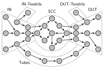
Figure 1: Bow-tie network topology. An example consisting of an in-section (IN), an out-section (OUT), a strongly connected component (SCC) or core, and tubes and tendrils (TT).

2 The Evolution of Centrality

2.1 Eigenvector Centrality

A lot of attention has been devoted to feedback-type centrality measures. These are based on the idea that a node is more central the more central its neighboring nodes themselves are. This notion leads to a set of equations which need to be solved simultaneously. In general, this type of centrality is also categorized as eigenvector centrality. The colloquialism “the importance of a node depends on the importance of the neighboring nodes” can be generically quantified as

$$c_{i}=\sum_{j}A_{ij}c_{j},$$ (1)

where $A$ is the adjacency matrix of the graph and $c_{i}$ denotes the centrality score of node $i$. More generally, by understanding $c$ as an eigenvector of the adjacency matrix, the last equation can be reformulated as

$$\lambda c=Ac,$$ (2)

with the eigenvalue $\lambda$. Note that Google’s search engine is based on a variant of eigenvector centrality, called PageRank Brin and Page (1998); Page et al. (1999).

Eigenvector-based centralities have been extensively studied in the literature. For instance, Bonacich and Lloyd (2001) introduced the following variation

$$\lambda c=\alpha Ac+e,$$ (3)

where $\alpha$ is a parameter and the vector $e$ represents an exogenous source. If $e$ is assumed to be a vector of ones, the solution of Eq. (3) can be related to the well-known centrality measure introduced in Katz (1953). Transitioning to weighted and directed graphs, a further refinement is given by the Hubbell index $c^{H}$ Hubbell (1965). Similarly to the term $e$ above, now the nodes are thought to posses an intrinsic importance $c^{0}$, to which the importance from being connected to neighboring nodes is added. In kinship to Eq. (3), the new centrality measure is defined as

$$c^{H}=Wc^{H}+c^{0},$$ (4)

where $W$ is the weighted adjacency matrix of the directed network. The solution is given by

$$c^{H}=(\mathbb{1}-W)^{-1}c^{0}.$$ (5)

For the matrix $(\mathbb{1}-W)$ to be non-negative and non-singular, a sufficient condition is that the Perron-Frobenius root is smaller than one, $\lambda(W)<1$. This is ensured by the requirement that in each strongly connected component $\mathcal{S}$ there exists at least one node $j$ such that $\sum_{i\in\mathcal{S}}W_{ij}<1$ Glattfelder and Battiston (2009). A similar centrality measure is found in Bonacich and Lloyd (2001).

A final variant of eigenvector centrality, setting the stage for the new measure to be introduced in the following, was defined in Bonacich (1987)

$$c_{i}(\alpha,\beta)=\sum_{j}(\alpha+\beta c_{j})A_{ij},$$ (6)

with the solution

$$c(\alpha,\beta)=\alpha(\mathbb{1}-\beta A)^{-1}Ae,$$ (7)

and $e$ being the column vector of ones and $\alpha,\beta$ the parameters to be chosen. This new centrality measure is essentially a refinement of Katz (1953) and Hubbell (1965). While it was originally defined in terms of the adjacency matrix $A$, it can be recast in the context of weighted and directed networks utilizing $W$. Note that $W_{ij}\in[0,1]$ and $\sum_{j}W_{ij}\leq 1$ (i.e., column-stochastic).

Additional information on eigenvector-based centrality variants and general node importance in complex networks can be found in Martin et al. (2014) and Lü et al. (2016), respectively.

2.2 Centrality in Ownership Networks

Prompted by the study of firms connected through a network of cross-shareholdings Brioschi et al. (1989); Brioschi and Paleari (1995) proposed an algebraic model, based on the input-output matrix methodology introduced to economics in Leontief (1966), to calculate the value of the firms. This methodology can be generalized to ownership networks and recast in the context of centrality Vitali et al. (2011); Glattfelder (2013). The corresponding equation defining the centrality $\chi$ is found to be

$$\chi=W\chi+Wv,$$ (8)

where $v$ is a vector representing the economic values of the nodes. Note, however, that $v$ can be a general non-topological node property, allowing the methodology to be applied to generic networks. Eq. (8) can be interpreted as follows: A node’s centrality score is given by the centrality scores of its neighbors plus the neighbors intrinsic properties. The solution is given by

$$\chi=(\mathbb{1}-W)^{-1}Wv=:\widetilde{W}v.$$ (9)

In other words, the centrality $\chi$ can be derived from the centrality $c(\alpha,\beta)$ from Eq. (7), by setting $\alpha=\beta=1$ and replacing the vector $e$ with the node properties defined by $v$.

Note that by using the series expansion

$$(\mathbb{1}-W)^{-1}=\mathbb{1}+W+W^{2}+W^{3}+\dots$$ (10)

one finds that

$$\widetilde{W}=(\mathbb{1}-W)^{-1}W=W(\mathbb{1}-W)^{-1}=\sum_{n=1}^{\infty}W^{n},$$ (11)

and the centrality matrix equation is

$$\widetilde{W}=W+W\widetilde{W}=W+\widetilde{W}W.$$ (12)

The centrality $\chi$ has a direct economic interpretation in terms of the value of the total portfolio of shareholders Glattfelder and Battiston (2019). The direct portfolio value is the aggregated monetary value representing a shareholder’s investments. In detail, it is defined for a shareholder $i$ as

$$p_{i}^{\text{dir}}=\sum_{j\in\Gamma(i)}W_{ij}v_{j},$$ (13)

where $\Gamma(i)$ is the set of indices of the neighbors of $i$, denoting all the companies in the portfolio. In the presence of a network, the notion of the indirect portfolio naturally arises Vitali et al. (2011); Glattfelder and Battiston (2019). This is the value found in the portfolio of portfolios. Specifically, the indirect portfolio value is found by traversing all the indirect paths reachable downstream from $i$

$$\begin{split}p_{i}^{\text{ind}}=&\sum_{j\in\Gamma(i)}\sum_{k\in\Gamma(j)}W_{ij}W_{jk}v_{k}+\cdots+\\ &\sum_{j_{1}\in\Gamma(i)}\sum_{j_{2}\in\Gamma(j_{1})}\cdots\sum_{j_{m-1}\in\Gamma(j_{m})}W_{ij_{1}}W_{j_{1}j_{2}}\cdots W_{j_{m-1}j_{m}}v_{j_{m}}+\cdots.\end{split}$$ (14)

As a result, one can assign the sum of the direct and indirect portfolio values to each shareholder, retrieving the total portfolio value

$$p_{i}^{\text{tot}}=p_{i}^{\text{dir}}+p_{i}^{\text{ind}}.$$ (15)

In matrix notation, this can be re-expressed as

$$p_{i}^{\text{tot}}=\sum_{n=1}^{\infty}W^{n}v.$$ (16)

By virtue of Eq. (11), it is found that $\chi=p_{i}^{\text{tot}}$.

In generic terms, Eq. (8) can be interpreted in the context of a system in which a resource (e.g., energy or mass) is flowing along the directed and weighted links of the network. In this picture, the intrinsic property value $v_{i}$ associated with the nodes represents the quantity of the resource produced by them. Now $\chi_{i}$ measures the inflow of this resource which accumulates in node $i$ from all the nodes downstream Glattfelder and Battiston (2009); Vitali et al. (2011).

In the following, this eigenvector centrality variant $\chi$ is called the access centrality, as it computes how much a node can access the intrinsic properties of all other nodes reachable downstream via the direct and indirect weighted links.

2.3 The Problems

It was realized that the access centrality $\chi$ suffers from undesirable issues. When the number of cycles in the network is large, for example in the core of the bow-tie, the measure computes overestimated results, due to the nodes’ intrinsic property value flowing many times through the cycles. A remedy was proposed, where, in essence, links are removed in the computation Baldone et al. (1998b); Rohwer and Pötter (2005). In detail, Eq. (12) is adapted as follows:

$$\widehat{W}_{ij}=W_{ij}+\sum_{k\neq i}\widehat{W}_{ik}W_{kj}.$$ (17)

This is equivalent to the introduction of a correction matrix Vitali et al. (2011); Glattfelder (2013)

$$\mathcal{D}=\textrm{diag}\left((\mathbb{1}-W)^{-1}\right)^{-1}.$$ (18)

Recall that $\textrm{diag}(A)$ is defined as the matrix of the diagonal elements of the matrix $A$. The components of $\mathcal{D}$ are

$$\mathcal{D}_{kk}=\frac{1}{(\mathbb{1}-W)^{-1}_{kk}},$$ (19a)

$$\mathcal{D}_{ij}=0,\quad i\neq j.\phantom{L}$$ (19b)

The corrected centrality matrix equation is

$$\widehat{W}=\mathcal{D}\widetilde{W},$$ (20)

and the new corrected centrality emerging from these manipulations is

$$\widehat{\chi}=\widehat{W}v.$$ (21)

As a result, in networks with cycles, by construction, $\widehat{\chi}_{i}\leq\chi_{i}$, otherwise $\widehat{\chi}_{i}=\chi_{i}$.

While this approach remedies the problem of overestimating the centrality due to cycles, it introduces another problem Vitali et al. (2011); Glattfelder (2013); Glattfelder and Battiston (2019). Cutting links in the network tames the cycles but makes root nodes dominant. A single root node in a bow-tie will have the highest corrected centrality score, regardless of the level of interconnectivity in the network. This is an undesirable effect, as the topology becomes irrelevant.

In Glattfelder and Battiston (2019) the authors propose a centrality measure addressing the above mentioned issues. In detail, an algorithm is described which computes the centrality score for each node, called the influence index $\xi$. For its computation, only the trails in the network are traversed. These are unique paths where each node is only visited once, thus terminating any further flow through cycles. In other words, for each iteration of the algorithm, the calculation considers the jump from node to node along the directed links until either a terminating leaf node is reached or a node that was visited some steps earlier is detected (the result of a cycle). In effect, the cycles in the network are cut. This algorithmically computed centrality represents a lower bound to the access centrality $\xi_{i}\leq\chi_{i}$. It should be noted that the influence index offers an algorithmic solution to the above mentioned problems. In this sense, it is a desirable centrality measure. The analytical bow-tie centrality emulates its properties.

2.4 An Example

Figure 2: Simple bow-tie network example with a high degree of interconnectedness of nodes in the SCC. All nodes have unit value $v_{i}=1$. Reproduced from Vitali et al. (2011).

Fig. 2 presents the bow-tie example introduced in Vitali et al. (2011); Glattfelder (2013). One finds for $v_{i}=1$

$$\chi=\left(\begin{array}[]{r}5\\ 49\\ 26\\ 48\\ 54\\ 0\end{array}\right),\ \widehat{\chi}=\left(\begin{array}[]{r}5.000\\ 4.900\\ 4.216\\ 4.571\\ 4.629\\ 0.000\end{array}\right),\ \xi=\left(\begin{array}[]{r}0.360\\ 2.600\\ 1.400\\ 2.520\\ 3.050\\ 0.000\end{array}\right).$$ (22)

This simple example highlights the mentioned problems. Namely, the overestimation of nodes in cycles affecting $\chi$ (i.e., $\chi_{2}$–$\chi_{5}$ having large values) and the dominance of root nodes affecting $\widehat{\chi}$ (i.e., $\widehat{\chi}_{1}$ being larger than $\widehat{\chi}_{2}$ – $\widehat{\chi}_{6}$). Moreover, it is confirmed that $\xi$ indeed acts as the lower bound for the calculations.

3 Deriving the Bow-Tie Centrality

While the access centrality $\chi$ and the corrected centrality $\widehat{\chi}$ are well-defined measures with clear interpretations, in practice, as mentioned, they have drawbacks when applied to weighted and directed networks with many cycles. Another measure, the influence index $\xi$, while remedying the problems can only be defined algorithmically. In essence, what is missing in the literature is an analytical expression (utilizing the adjacency matrix) which allows a centrality score to be computed that is similar to the influence index (and hence is also not plagued by the problems detailed above) and which can be applied to bow-tie networks (with intrinsic node properties). In the following, such a new centrality measure is derived.

Let the auxiliary matrix $V$ be defined as

$$V=(\mathbb{1}-W)^{-1}.$$ (23)

This allows some equations to be re-expressed. Eq. (11) is now

$$\widetilde{W}=WV$$ (24)

and Eq. (20) becomes

$$\widehat{W}=\mathcal{D}\widetilde{W}=\mathcal{D}WV,$$ (25)

highlighting how the correction matrix impacts the original centrality matrix. However, the correction matrix $\mathcal{D}$ could be applied at a different position in Eq. (25), unveiling yet another corrected eigenvector centrality variant

$$\overline{W}=W\mathcal{D}V.$$ (26)

In essence, the non-commutative nature of matrix multiplication $\mathcal{D}W\neq W\mathcal{D}$ results in two analytical expressions. It should be noted that in mathematics and physics, non-commutative behavior is a source of rich structure Connes (1994); Seiberg and Witten (1999); Douglas and Nekrasov (2001).

For the new centrality measure, one finds

$$\overline{W}=W\mathcal{D}(\mathbb{1}-W)^{-1}=W\mathcal{D}\left(W(\mathbb{1}-W)^{-1}+\mathbb{1}\right)=W\mathcal{D}(\widetilde{W}+\mathbb{1})=W(\widehat{W}+\mathcal{D}),$$ (27)

by noting that from Eq. (10)

$$\mathbb{1}+W+W^{2}+\dots=W(\mathbb{1}+W+W^{2}+\dots)+\mathbb{1}.$$ (28)

In a nutshell, the new centrality matrix is

$$\overline{W}=WW^{\ast},$$ (29)

with

$$W^{\ast}=\widehat{W}+\mathcal{D},$$ (30)

or in scalar notation

$$W^{\ast}_{ij}=\begin{cases}1,&i=j,\\ \widehat{W}_{ij},&i\neq j.\end{cases}$$ (31)

The final resulting centrality measure, called the bow-tie centrality, is

$$\zeta=\overline{W}v.$$ (32)

It is an analytical expression that does not overestimate the importance of nodes in cycles and root nodes.

In the example seen in Fig. 2 one finds

$$\chi=\left(\begin{array}[]{r}5\\ 49\\ 26\\ 48\\ 54\\ 0\end{array}\right),\ \zeta=\left(\begin{array}[]{r}0.500\\ 5.465\\ 2.443\\ 4.329\\ 7.023\\ 0.000\end{array}\right),\ \xi=\left(\begin{array}[]{r}0.360\\ 2.600\\ 1.400\\ 2.520\\ 3.050\\ 0.000\end{array}\right).$$ (33)

Theorem 1.

The bow-tie centrality measure $\zeta$ is bounded by the access centrality $\chi$ and the influence index $\xi$:

$$\chi_{i}\geq\zeta_{i}\geq\xi_{i}.$$ (34)

Proof.

Recall that the adjacency matrix of an ownership network is column-stochastic if all the ownership information is known. In general, $\sum_{j}W_{ij}\leq 1$ and $W_{ij}\in[0,1]$. The matrix $V$ is defined in Eq. (23) and from Eq. (10), $V_{ij}\geq 0$.

The first inequality translates into $\widetilde{W}_{ij}v_{j}\geq\overline{W}_{ij}v_{j}$. Componentwise

$$\overline{W}_{ij}=\sum_{k,l}W_{ik}\mathcal{D}_{kl}V_{lj}\stackrel{{\scriptstyle Eq.(\ref{eq:Dscalar})}}{{=}}\sum_{k}W_{ik}\mathcal{D}_{kk}V_{kj}\leq\sum_{k}W_{ik}V_{kj}=\widetilde{W}_{ij}.$$ (35)

The inequality follows by observing that from Eq. (19a), $\mathcal{D}_{kk}=V_{kk}^{-1}\in]0,1]$, because $V_{kk}=1+W_{kk}+\dots\geq 1$, and thus $\mathcal{D}_{kk}V_{kj}\leq V_{kj}$.

The second inequality arises by construction. In the absence of cycles, all the centrality measures are identical. In the presence of cycles, the influence index algorithm only traverses the trails in the network. These are unique paths where each node is only visited once, thus terminating any further flow through cycles. In other words, cycles are never actually fully traversed and the computation stops one node before completion. This is the minimum possible contribution from cycles. The bow-tie centrality is defined using powers of $W$, resulting in paths of various lengths being considered. In essence, contributions from cycles are incorporated in the computation, exceeding the bare minimum arising from the trails. It should be noted that if a centrality measure yields lower values than the influence index this means that information from the cycles has been lost in the computation. ∎

4 Empirical Application

A prototypical bow-tie network can be found in the global ownership network Glattfelder and Battiston (2019). Ownership networks are comprised of economic actors which are connected via ownership relations (i.e., by holding a percentage of a corporations’ equity). Shareholders can be other firms, natural persons, families, foundations, research institutes, public authorities, states, and government agencies. Ownership networks are directed and weighted, and some of the corporations have an intrinsic node property, coming in the guise of an economic value (e.g., the firm’s operating revenue in USD). Typical for ownership networks is the emergence of a tiny but highly interconnected core (SCC) of influential shareholders. Hence, this is an ideal real-world use-case for the bow-tie centrality measure.

The global ownership information is taken from Bureau van Dijk’s Orbis database. In Glattfelder and Battiston (2019), six yearly network snapshots were constructed and analyzed from this. Here, we focus on the largest connected component of 2012. In detail, we analyzes the IN, the SCC, and the OUT, omitting the TT. From a set of 35,839,090 nodes and 27,307,642 links, the largest connected component was identified as being comprised of 5,933,836 nodes. In the following, a subnetwork of the 2012 global ownership network is analyzed. By considering all of the IN and SCC nodes, plus all OUT nodes with an operating revenue larger or equal to USD 100,000,000 (i.e., $v_{i}^{\text{out}}\geq 100$ million), a reduced ownership network is retrieved. It contains 64,266 nodes and 540,405 links. In Table 1 the bow-tie component sizes are shown. There are 52,001 nodes with an operating revenue $v_{i}>0$ contained in the reduced network, totaling USD 84,287,655,740,000. This represents 66.30% of the total global operating revenue of the entire global ownership network, which is approximately USD 127 trillion Glattfelder and Battiston (2019).

IN	13,374
SCC	2,554
OUT	48,338
Total	64,266

Table 1: Bow-tie components of the reduced global ownership network of 2012. The number of nodes in the various components of the network are shown, totaling 64,266 nodes. The different centrality measures are applied to this empirical network.

4.1 Comparing the Rankings

For the empirical analysis, all the discussed centrality measures are computed for this network. Namely

1. the access centrality $\chi=(\mathbb{1}-W)^{-1}Wv=\widetilde{W}v$

2. the corrected centrality $\widehat{\chi}=\mathcal{D}\widetilde{W}v=\widehat{W}v$

3. the bow-tie centrality $\zeta=W(\widehat{W}+\mathcal{D})v=\overline{W}v$

4. the algorithmic influence index $\xi$.

As a result, there are six possible comparisons of the rankings. By utilizing the Jaccard index, a statistic used for assessing the similarity of sets Jaccard (1912), such a comparison can be quantified. The index is defined as

$$\mathcal{J}(A,B)={{|A\cap B|}\over{|A\cup B|}},$$ (36)

for two sets $A$ and $B$. A value of one indicates a total overlap of the sets, while zero denotes no similarity.

The truncated Jaccard index $\mathcal{J}_{n}$ is employed to uncover the similarity between the $n$ highest ranked nodes of two centrality measures Glattfelder and Battiston (2019). For instance, $\mathcal{J}_{n}(\zeta,\chi)$ compares the bow-tie centrality with the access centrality for the firs $n$ nodes ranked by centrality. $\mathcal{J}_{n}$ can then be plotted for all centrality comparisons of all lengths.

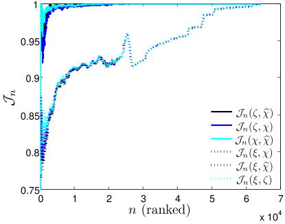
Figure 3: Jaccard indices comparing the centrality rankings. The similarity of the four network centrality measures is visualized by computing the Jaccard index $\mathcal{J}_{n}$ for all ranked sets of length $n=1,\dots,64,266$. The $x$-axis shows the number of centrality-ranked nodes, where $n=1$ represents the node with the highest centrality. See discussion in text.

Fig. 3 shows the results of this computation. The three analytical centrality measures $\chi,\widehat{\chi}$, and $\zeta$ display a high similarity among themselves. In contrast, the algorithmic centrality $\xi$ shows a pronounced dissimilarity with respect to the analytical measures. The two centrality variants based on $\chi$, utilizing the correction matrix $\mathcal{D}$, show the highest similarity. Symbolically, $\zeta\sim\widehat{\chi}$. This implies that the way the bow-tie centrality adjusts for cycles yields similar results as the corrected centrality. Recalling that both $\chi$ and $\widehat{\chi}$ are affected by topology-dependent issues, the bow-tie centrality $\zeta$ emerges as a superior analytical centrality measure, while still accurately reflecting the behavior of the access centrality $\chi$.

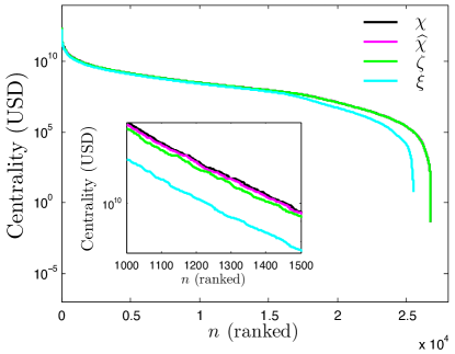
Figure 4: Ranked centrality value semi-log plots. For all four centrality measures, their monetary value is shown for each node. The inset shows the details for 500 nodes ranked between 10,000 and 15,000.

By further comparing the bow-tie centrality to the influence index, the following is revealed. Of the 64,266 nodes in the reduced ownership network, 26,758 have a non-zero analytical centrality. Symbolically, $|\{\zeta_{i}>0\}|=|\{\chi_{i}>0\}|=|\{\widehat{\chi}_{i}>0\}|=26,758$. For the algorithmic influence index, the number is the following $|\{\xi_{i}>0\}|=25,512$. From Theorem 1 it is known that the influence index is a lower bound for the bow-tie centrality, i.e., $\zeta_{i}\geq\xi_{i}$. In Fig. 4 the monetary values of each node for each centrality variant is shown in ranked plots. Indeed, in the network at hand, the algorithmic centrality is below the analytical ones, which all have similar values.

4.2 Top-Ten Rankings

In Glattfelder and Battiston (2019) the entire global ownership network was analyzed. In other words, the centrality scores for 35,839,090 nodes was algorithmically evaluated (i.e., $\xi_{i}$). From a computational perspective, calculating the analytical centrality measures for such a matrices can be challenging.

However, by focusing on the core structures of the network, a smaller representation can be found. The reduced ownership network analyzed here, comprised of 64,266 nodes, represents 66.30% of the total global operating revenue. A key question to be answered is how representative this subnetwork is? Moreover, as a different centrality measure was used, are the two resulting rankings comparable? In other words, how similar is the influence index, computed for the entire network, to the bow-tie centrality, calculated for the reduced network?

In Table 2 the two centralities are compared for the top-ten list. While the individual rankings are expected to change, the group of actors is very similar. Both centrality measures crucially identify a similar set of most relevant nodes in the network. Furthermore, although there is not as much value in the reduced network, the bow-tie centrality is a less conservative estimation resulting in higher centrality values.

In summary, this result can be seen as evidence that it suffices to focus on the relevant part of the network for quantitative analysis. In this case it was a combination of topology (all the nodes in the IN and SCC) and value (nodes in the OUT with a minimum of 100 million operating revenue in USD). For rapid testing of ideas and approximating indicators, this approach can be invaluable. The analytical bow-tie centrality is straightforward to apply while the implementation of the algorithmic influence index required the utilization of a graph database.

Influence Index    (entire network)		Bow-Tie Centrality    (reduced network)
Name	$\xi$ (t USD)	Name	$\zeta$ (t USD)
BLACKROCK INC	2.177	BLACKROCK INC	2.421
VANGUARD GROUP INC	1.314	VANGUARD GROUP INC	1.516
GOVERNMENT OF NORWAY	1.220	STATE STREET CORP	1.359
SASAC	1.210	GOVERNMENT OF NORWAY	1.299
CAPITAL GROUP COMPANIES	1.201	CAPITAL GROUP COMPANIES	1.246
STATE STREET CORP	1.190	BPCE SA	1.155
GOVERNMENT OF FRANCE	0.982	FMR LLC	1.096
FMR LLC	0.955	BARCLAYS PLC	0.796
BARCLAYS PLC	0.675	JP MORGAN CHASE & CO	0.715
ROYAL DUTCH SHELL PLC	0.619	T. ROWE PRICE GROUP INC	0.643

Table 2: Comparing the top-ten rankings. The exhaustive results taken from (Glattfelder and Battiston, 2019) are seen on the left-hand side. The right-hand side shows the results from the reduced network utilizing the bow-tie centrality from Eq. (32). The values are in trillion USD.

5 Conclusion

Which are the most important nodes in a network? This question has a long history in network science and there are different ways of approaching it. For instance, algorithms can be developed which traverse the network and compute the centrality scores of the nodes. While such an approach requires a computational framework, it can be applied to very large networks. A more classical approach is to utilize equations. In this analytical context many centrality measures have been proposed. However, for a relevant class of directed and weighted real-world networks, characterized by a bow-tie topology, these centralities suffer from drawbacks. Specifically, the emergence of cycles represents a formidable challenge.

We introduce a novel centrality measure ideally applied to networks displaying a bow-tie topology. The quantity represents a final iteration in a stream of research originating from the study of ownership networks Brioschi et al. (1989); Brioschi and Paleari (1995); Baldone et al. (1998a); Rohwer and Pötter (2005); Glattfelder and Battiston (2009); Vitali et al. (2011); Glattfelder (2013); Glattfelder and Battiston (2019). The new centrality measure can be applied in general to weighted and directed complex networks, where the nodes carry an intrinsic non-topological degree of freedom. The ideal domain of application are such networks, where the bow-tie contains important nodes. Here, older centrality measures overestimate the relevance of such nodes (in the SCC and IN bow-tie components) and blur important features. Indeed, the bow-tie centrality yields a precise score for every node in the network, regardless of its location in the bow-tie.

The bow-tie centrality can be clearly motivated analytically and does not possesses the undesirable features plaguing older variants (such as the access and corrected centralities). Comparing these different centrality measure to each other reveals that the novel bow-tie centrality achieves this while still capturing the desired features of ownership-inspired eigenvector centralities. In essence, this centrality represents the analytical counterpart to an algorithmic implementation used to decode empirical ownership networks, namely the influence index Glattfelder and Battiston (2019) (or an older, more cumbersome variant found in Vitali et al. (2011)).

Finally, it was demonstrated that large networks can be reduced to smaller subsets which, when analyzed, show very similar properties as the whole. In essence, the characteristic features of a network are encoded in the subnetwork of important nodes, making the detection of this backbone crucial. To this aim, better centrality measures are important.

References

- Baldone et al. [1998a] S. Baldone, F. Brioschi, and S. Paleari. Ownership measures among firms connected by cross-shareholdings and a further analogy with input-output theory. 4th JAFEE International Conference on Investment and Derivatives, 1998a.
- Baldone et al. [1998b] S. Baldone, F. Brioschi, and S. Paleari. Ownership Measures Among Firms Connected by Cross-Shareholdings and a Further Analogy with Input-Output Theory. 4th JAFEE International Conference on Investment and Derivatives, 1998b.
- Benevenuto et al. [2009] F. Benevenuto, T. Rodrigues, V. Almeida, J. Almeida, and K. Ross. Video interactions in online video social networks. ACM Transactions on Multimedia Computing, Communications, and Applications (TOMCCAP), 5(4):30, 2009.
- Bonacich [1972] P. Bonacich. Factoring and weighting approaches to status scores and clique identification. Journal of Mathematical Sociology, 2(1):113–120, 1972.
- Bonacich [1987] P. Bonacich. Power and centrality: A family of measures. The American Journal of Sociology, 92(5):1170–1182, 1987.
- Bonacich and Lloyd [2001] P. Bonacich and P. Lloyd. Eigenvector-Like Measures of Centrality for Asymmetric Relations. Social Networks, 23(3):191–201, 2001.
- Borgatti and Everett [2006] S. Borgatti and R. Everett. A Graph-Theoretic Perspective on Centrality. Social Networks, 28(4):466–484, 2006.
- Brin and Page [1998] S. Brin and L. Page. The Anatomy of a Large-Scale Hypertextual Web Search Engine. Computer Networks and ISDN Systems, 30(1-7):107–117, 1998.
- Brioschi and Paleari [1995] F. Brioschi and S. Paleari. How Much Equity Capital Did the Tokyo Stock Exchange Really Raise. Financial Engineering and the Japanese Markets, 2(3):233–258, 1995.
- Brioschi et al. [1989] F. Brioschi, L. Buzzacchi, and M. Colombo. Risk Capital Financing and the Separation of Ownership and Control in Business Groups. Journal of Banking and Finance, 13(1):747 – 772, 1989.
- Broder et al. [2000] A. Broder, R. Kumar, F. Maghoul, P. Raghavan, S. Rajagopalan, S. Stata, A. Tomkins, and J. Wiener. Graph Structure in the Web. Computer Networks, 33:309, 2000.
- Connes [1994] A. Connes. Noncommutative geometry. Academic Press, San Diego, 1994.
- Donato et al. [2008] D. Donato, S. Leonardi, S. Millozzi, and P. Tsaparas. Mining the Inner Structure of the Web Graph. Journal of Physics A: Mathematical and Theoretical, 41(22):224017, 2008.
- Douglas and Nekrasov [2001] M. R. Douglas and N. A. Nekrasov. Noncommutative field theory. Reviews of Modern Physics, 73(4):977, 2001.
- Freeman [1978] L. Freeman. Centrality in Social Networks Conceptual Clarification. Social Networks, 1:215–239, 1978.
- Freeman [2008] L. Freeman. Going the Wrong Way on a One-Way Street: Centrality in Physics and Biology. Journal of Social Structure, 9(2), 2008.
- Fujiwara and Aoyama [2008] Y. Fujiwara and H. Aoyama. Large-scale structure of a nation-wide production network. The European Physical Journal B-Condensed Matter and Complex Systems, pages 1–16, 2008.
- Glattfelder [2013] J. B. Glattfelder. Decoding Complexity: Uncovering Patterns in Economic Networks. Springer, Heidelberg, 2013.
- Glattfelder and Battiston [2009] J. B. Glattfelder and S. Battiston. Backbone of complex networks of corporations: The flow of control. Physical Review E, 80(3):036104, 2009.
- Glattfelder and Battiston [2019] J. B. Glattfelder and S. Battiston. The architecture of power: Patterns of disruption and stability in the global ownership network. SSRN, 2019.
- Hubbell [1965] C. Hubbell. An input-output approach to clique identification. Sociometry, 28(4):377–399, 1965.
- Jaccard [1912] P. Jaccard. The distribution of the flora in the alpine zone. New Phytologist, 11(2):37–50, 1912.
- Katz [1953] L. Katz. A new status index derived from sociometric analysis. Psychometrika, 18(1):39–43, 1953.
- Leontief [1966] W. Leontief. Input-Output Economics. Oxford University Press, Oxford, 1966.
- Lü et al. [2016] L. Lü, D. Chen, X.-L. Ren, Q.-M. Zhang, Y.-C. Zhang, and T. Zhou. Vital nodes identification in complex networks. Physics Reports, 650:1–63, 2016.
- Martin et al. [2014] T. Martin, X. Zhang, and M. E. Newman. Localization and centrality in networks. Physical review E, 90(5):052808, 2014.
- Newman et al. [2006] M. Newman, A. Barabási, and D. Watts. The Structure and Dynamics of Networks. Princeton University Press, Princeton, 2006.
- Page et al. [1999] L. Page, S. Brin, R. Motwani, and T. Winograd. The pagerank citation ranking: Bringing order to the web. Technical report, Stanford InfoLab, 1999.
- Rohwer and Pötter [2005] G. Rohwer and U. Pötter. Transition Data Analysis User’s Manual. Ruhr-University Bochum, 2005.
- Schweitzer et al. [2009] F. Schweitzer, G. Fagiolo, D. Sornette, F. Vega-Redondo, A. Vespignani, and D. White. Economic Networks: The New Challenges. Science, 325(5939):422, 2009.
- Seiberg and Witten [1999] N. Seiberg and E. Witten. String theory and noncommutative geometry. Journal of High Energy Physics, 1999(09):032, 1999.
- Vitali et al. [2011] S. Vitali, J. B. Glattfelder, and S. Battiston. The network of global corporate control. PLoS one, 6(10):e25995, 2011.
- Zhang et al. [2007] J. Zhang, M. Ackerman, and L. Adamic. Expertise networks in online communities: structure and algorithms. In Proceedings of the 16th international conference on World Wide Web, pages 221–230. ACM, 2007.