Phys. Rev. B, in press arXiv:1911.00923 An On-Site Density Matrix Description of the Extended Falicov–Kimball Model at Finite Temperatures

Abstract

We propose a single-site mean-field description, an analogue of Weiss mean field theory, suitable for narrow-band systems with correlation-induced hybridisation at finite temperatures. Presently this approach, based on the notion of a fluctuating on-site density matrix (OSDM), is developed for the case of extended Falicov-Kimball model (EFKM). In an EFKM, an excitonic insulator phase can be stabilised at zero temperature. With increasing temperature, the excitonic order parameter (interaction-induced hybridisation on-site, characterised by the absolute value and phase) eventually becomes disordered, which involves fluctuations of both its phase and (at higher $T$) its absolute value. In order to build an adequate finite-temperature description, it is important to clarify the nature of degrees of freedom associated with the phase and absolute value of the induced hybridisation, and correctly account for the corresponding phase-space volume. We show that the OSDM-based treatment of the local fluctuations indeed provides an intuitive and concise description (including the phase-space integration measure). This allows to describe both the lower-temperature regime where phase fluctuations destroy the long-range order, and the higher temperature crossover corresponding to a decrease of the absolute value of hybridisation. In spite of the rapid progress in the studies of excitonic insulators, a unified picture of this kind has not been available to date. We briefly discuss recent experiments on ${\rm Ta_{2}NiSe_{5}}$ and also address the amplitude mode of collective excitations in relation to the measurements reported for ${\rm 1}T-{\rm TiSe}_{2}$. Both the overall scenario and the theoretical framework are also expected to be relevant in other contexts, including the Kondo lattice model.

I INTRODUCTION

Interaction-induced pairing commonly occurs in many different contexts including excitonic and Kondo insulators and superconductivity. This can involve either particle-hole or particle-particle pairs, and gives rise to an induced hybridisation or to a superconducting pairing amplitude, both of which can be viewed as scalar products between formerly orthogonal many-body states, i.e., as off-diagonal elements of some density matrix. The corresponding systems are characterised by the ratio of the induced spectral gap (or pair binding energy) to the bandwidth energy scales. The case of small binding energy (weak interaction) corresponds to the well-known BCS picture, where the crucial rôle is played by restructuring of the quasiparticle spectra in the vicinity of the Fermi level only. Broadly speaking, this case is amenable to a long-wavelength perturbative treatment, leading to the familiar results. The opposite limiting case, which is commonly referred to as that of BEC (Bose–Einstein condensation), is typically realised in the narrow-band systems and continues to command much attention from experimental and theoretical standpoints. It has been suggested that this BEC physics might be relevant for Kondo lattices and heavy-fermion compoundsPiers ; Lonzarich , for high-temperature superconductors (“pre-formed pairs” scenarioNSR ; Randeria ; Kathy ), as well as for various aspects of excitonic-insulating behaviour in narrow-band systemsSmTm ; 1TTiSe2 ; Kogar2017 (including “electronic ferroelectricity”Portengen ). One may also note a rather direct connexion with much discussed “Higgs bosons” in correlated electron systemsHiggs , due to the difference in the energy cost of phase and amplitude fluctuations of, e.g., induced hybridisation.

In the BEC regime, there are two distinct energy scales, corresponding to the energy of strongly-bound excitons or pairs and to their interaction with each other. This gives rise to a peculiar evolution of the system with increasing temperature, as will be further discussed below. Importantly, the BEC pairing is not a phenomenon which concerns only the carriers in the vicinity of the Fermi level, and new theoretical tools are needed (and were indeed suggested, see, e.g., Refs. Piers, ; Randeria, ; Kathy, ; Apinyan, ) in order to study the behaviour of a system in this regime. Owing to a small spatial size of an exciton or a pair, it appears highly desirable to construct a simplified local mean-field description of a single-site type, an analogue of an elementary Weiss mean field approach familiar from the theory of magnets. Hitherto, this important benchmark appears to be missing, and our present objective is to begin filling this gap.

Arguably, the simplest situation where this BEC regime arises is that of the excitonic insulating state in an extended spinless Falicov-Kimball model (EFKM). In this paper, we develop a single-site mean-field description for this case, while adaptation of the method and of the insights to other systems is relegated to future work. It should be noted that Falicov–Kimball model throughout its history attracted a massive research effortZlatic , owing to its simplicity, peculiarity, and physical relevance. The possibility of an ordered excitonic state in this model was originally conjectured some 43 years agoKhomskii76 , and a brief review of more recent literature can be found, e.g., in Ref. prb12, . In particular, variegated analytical and numerical methods were employed to investigate exciton condensationBatista04 ; condEFKM , and more generally the BCS–BEC crossoverBECEFKM , in the EFKM.

The spinless Falicov–Kimball model properFK involves fermions $d_{i}$ and $c_{i}$ in the localised and itinerant bands, interacting via a Coulomb repulsion $U$ on-site:

$${\cal H}=-\frac{t}{2}\sum_{\langle ij\rangle}\left(c^{\dagger}_{i}c_{j}+c^{\dagger}_{j}c_{i}\right)+E_{d}\sum_{i}d^{\dagger}_{i}d_{i}+U\sum_{i}c^{\dagger}_{i}d^{\dagger}_{i}d_{i}c_{i}\,,$$ (1)

where $E_{d}$ is the bare energy of the localised band. We are interested in the case where $U$ is, broadly speaking, of the same order of magnitude as the bare hopping amplitude $t$, and we choose the units where $t$ and the period of the ($d$-dimensional hypercubic) lattice are equal to unity. We also set $\hbar=k_{B}=1$.

In order to stabilise the state with a large on-site hybridisation at $T=0$,

$$\Delta_{i}\equiv|\Delta_{i}|{\rm e}^{{\rm i}\varphi_{i}}=\langle c^{\dagger}_{i}d_{i}\rangle\,,$$ (2)

one must extend the Falicov–Kimball model by adding a perturbation of general formCzycholl99 ; Farkasovsky08 ; Schneider08 ; prb12

$$\delta{\cal H}= \!\!\!\!\!\!\left\{-\frac{t^{\prime}}{2}\sum_{\langle ij\rangle}d^{\dagger}_{i}d_{j}+V_{0}\sum_{i}c^{\dagger}_{i}d_{i}-\frac{V_{1}}{2}\sum_{\langle ij\rangle}\left(c^{\dagger}_{i}d_{j}+c^{\dagger}_{j}d_{i}\right)-\right.$$ (3)

$$\!\!\!\!\!\!\left.-\frac{V_{2}}{2}\sum_{\langle ij\rangle}\left([\vec{R}_{j}-\vec{R_{i}}]\cdot\vec{\Xi}\right)\left(c^{\dagger}_{i}d_{j}-c^{\dagger}_{j}d_{i}\right)\right\}+{\rm H.c.}\,,$$

where $t^{\prime}$ is the $d$-band hopping and $V_{0}$, bare on-site hybridisation. $V_{1}$ ($V_{2}$) is the spatially-even (odd) nearest-neighbour hybridisation, as appropriate for the case where the two original bands have the same (opposite) parity. $\vec{R}_{i}$ is the radius-vector of a site $i$, and $\vec{\Xi}=\sum_{\alpha=1}^{d}\hat{\mathbf{x}}_{\alpha}$, sum of Cartesian unit vectors. For $t^{\prime}=0$, the net Hamiltonian, Eqs. (1) and (3), coincides with that of a spinless periodic Anderson model, while in the opposite case of $V_{0,1,2}=0$ the EFKM becomes identical with the asymmetric Hubbard model, where the hopping coefficients for spin-up ($c_{i}$) and spin-down ($d_{i}$) electrons differ, and $E_{d}$ in Eq. (1) is proportional to the Zeeman splitting.

In a broad range of values of parameters of Eq. (1), including any of the four terms in Eq. (3) with an appropriate sign (i.e., $t^{\prime}<0$, $V_{0}<0$, $V_{1}$ with $V_{1}E_{d}<0$, or $V_{2}$ of any sign) would result at $T=0$ in an ordered excitonic state with a uniform $|\Delta_{i}|=\Delta$ and $\varphi_{i}=0$ (when only $t^{\prime}$ differs from $0$, $\varphi_{i}$ can take any constant value; we choose the latter to be equal to zero). This is a mixed-valence state with uniform band occupancies,

$$n_{c,i}\equiv\langle c^{\dagger}_{i}c_{i}\rangle=n_{c}\,,\,\,\,n_{d,i}\equiv\langle d^{\dagger}_{i}d_{i}\rangle=n_{d}\,.$$ (4)

The absolute value of the corresponding perturbation parameter must be larger than a certain critical value ($|t^{\prime}_{cr}|$, etc.). Depending on the parameters of the Hamiltonian, Eq. (3), the value of $\Delta$ (at least at half-filling, $n=n_{c}+n_{d}=1$) may be large, $\Delta\stackrel{{\scriptstyle<}}{{\sim}}1/2$. With decreasing perturbation strength (e.g., the parameter $|t^{\prime}|$ is decreased toward $|t^{\prime}_{cr}|$) the value of $\Delta$ does not tend to zero. Rather, at a critical point (such as $|t^{\prime}|=|t^{\prime}_{cr}|$) a new, presumably charge-ordering order parameter arises via a second-order phase transitionFarkasovsky08 ; prb12 ; Apinyan , destroying the uniformly ordered excitonic state. The critical value $t^{\prime}_{cr}$ [as well as critical values of the hybridisations $V_{0}$, $V_{1}$, or $(V_{2})^{2}$] turns out to be numerically small, some two orders of magnitude smaller than the bare hopping $t$. Therefore, a useful insight can often be gained by either treating $\delta{\cal H}$ perturbatively or even technically neglecting its effects by keeping only the leading-order term in the calculation.

The behaviour of the system at finite $T$ is crucially dependent on the two energy scales characterising the ordered excitonic state at $T=0$. The first one is the hybridisation-induced energy gap, notably the indirect one, which in cases where $U$ is not very large can be roughly estimated as

$$G\sim 2U^{2}\Delta^{2}/d$$ (5)

(see Sec. II; note that the bandwidth of the unhybridised itinerant band equals $2d$, twice dimensionality of the system), and can be an order of magnitude smaller than the direct gap,

$$u=2U\Delta\,.$$ (6)

While the value of $G$ at $T=0$ determines the crossover temperature $T_{*}$, a much smaller scale of the low-lying collective excitationsprb12 ; Jerome controls critical temperature $T_{cr}$ of the ordering transition (corresponding to the Bose–Einstein condensation of the excitonic gas). The value of $T_{cr}$ can be estimatedprb12 as $(T_{cr})^{2}\sim|t^{\prime}|(|t^{\prime}|-|t^{\prime}_{cr})$ [or $(T_{cr})^{2}\sim V_{2}^{2}(V_{2}^{2}-V_{2,cr}^{2})$, etc., when hybridisationextfield dominates $\delta{\cal H}$]. While the excitonic long-range order is lost already at $T=T_{cr}$ (where the phases $\varphi_{i}$ become disordered), the average value $\Delta(T)$ of $|\Delta_{i}|$ remains finite, and the state of the system can be termed disordered electronic insulator. It is also variously called “excitonic liquid” or “excitonic gas” (as opposed to “excitonic condensate” at $T<T_{cr}$), as the relatively stable excitons persist in equilibrium without a condensate. Since this state is not associated with a symmetry breaking, it fades away via a smooth crossover with increasing $T$ beyond $T_{*}$, when the thermal fluctuations of $|\Delta_{i}|$ become comparable to $\Delta(T)$. Above $T_{*}$, excitons can no longer be considered stable, as they are being formed and destroyed rapidly in the course of fluctuations.

Historically, the investigations of EFKM at finite temperatures started with extending the pioneering Hartree–Fock decoupling approach of Ref. Khomskii76, to finite $T$. However, this method misses the lower energy scale altogether (also at $T=0$), yielding a second-order phase transition at a certain $T_{*}\sim G$, above which $\Delta(T)$ vanishes (see, e.g., Ref. Schneider08, ). On the other hand, qualitative picture outlined in the previous paragraph is substantiated by a more advanced self-consistent treatment of Ref. Apinyan, . Still, it appears that due to the restrictions of a specific mean-field approach used in the latter reference (involving functional integrals technique with certain topological complications stemming from the nature of the phase variable $\varphi_{i}$), its conclusions imply a distinct transition at $|T_{*}|$, as opposed to a smooth crossover expected on symmetry grounds.

As already mentioned, it appears highly desirable to try and construct a more intuitive treatment of a single-site type. In addition, one expects that the behaviour of the system in the most interesting crossover regime around $T_{*}$ is strongly affected by the short-range fluctuations, which might not be dealt with accurately within the long-wavelength (continuum) approach of Ref. Apinyan, . Finally, one can anticipate that once an adequate single-site mean-field scheme is developed for the EFKM, it can be adapted for the entire family of related systems, as discussed in the beginning of this section.

In constructing our finite-temperature single-site mean field approach, we make use of the known properties of the conventional Hartree–Fock solutionKhomskii76 ; Farkasovsky08 ; prb12 ; Schneider08 for the EFKM. These are summarised in Sec. II, where we also outline our general strategy, which requires taking into account thermal fluctuations of the local quantities $\Delta_{i}$ and $n_{d,i}$. While the values of hybridisation and band occupancies can be deduced from the (fluctuating) on-site density matrix (OSDM), our Hamiltonian is non-local, and in order to calculate the energy cost of a local fluctuation one needs a fuller knowledge of the quantum state of the system. The form of the wave functions corresponding to such local fluctuations is obtained, under broad assumptions, in Sec. III. The emergent correspondence between the OSDM and the states of the system is also used in order to find the phase-space volume corresponding to a local fluctuation. While finding the suitable integration measure in the space of quantum states appears complicated, an established notionBengsston of measure in the space of density matrices (Bures measure) can be readily adapted to the case at hand. This is accomplished in Sec. IV, completing the description of our mean-field scheme. We note that the development in Secs. III and IV appears rather general, and may prove useful beyond the Hartree–Fock approximation for the wave functions, utilised elsewhere throughout the paper.

The actual application of the technique introduced in Secs. II–IV begins in Sec. V with the analysis of the low-temperature behaviour, including the ordering transition at $T_{cr}$. While in this case one does not expect any single-site approach to yield an accurate description, we do find a second-order phase transition with the value of $T_{cr}$ controlled by the parameters of the perturbation, Eq. (3).

The behaviour of the EFKM in the high-temperature phase-disordered state, including the crossover region at $T\sim T_{*}$, is considered in Sec. VI. It appears that the results obtained there are both reliable (except when the approach fails due to the underlying Hartree–Fock approximation becoming invalid, Sec. VI.1) and new, providing the first quantitative description of the crossover region in the EFKM. This description of the phase-disordered state appears rather workable from the point of view of, e.g., prospective calculation of the transport properties.

In Sec. VII, the emerging picture is discussed in the context of the ongoing experimental search for excitonic insulators. While the experimental situation is still uncertain (see, e.g.,, a brief review of recent literature on ${\rm Ta_{2}NiSe_{5}}$ in Sec. VII.1), this is likely to change in the near future, enabling a more meaningful comparison with the theoretical insights. We also include a rather qualitative treatment of collective excitations (amplitude mode, Sec. VII.2) in light of recent experimentsKogar2017 .

One can expect that potential applications of the technique developed in this paper extend beyond those rather limited aspects considered in Secs. VI and VII, both for the EFKM and in the context of other systems. This issue is, among others, discussed in Sec. VIII.

The reader interested mostly in our results for the behaviour of the EFKM at finite temperature might want to skip the description of the formalism in Secs. III–IV. On the other hand, those interested specifically in the OSDM-based mean-field technique could, at a first reading, proceed directly from Sec. IV to Sec. VIII.

Overall, the discussion in the paper is rather self-contained, as the Appendices supply necessary technical details for Secs. III, V, and VI. While some preliminary considerations were reported earlier in Ref. physicab18, , the technique used there is largely inadequate. Hence, Ref. physicab18, is completely superseded by the present paper.

II SINGLE-SITE MEAN-FIELD SCHEME AND THE HARTREE–FOCK SOLUTION

An ordered excitonic insulator state at $T=0$ is characterised by the uniform values of $n_{c,i}$, $n_{d,i}$, and (real positive) $\Delta_{i}$. At a finite temperature, these begin to fluctuate, and as long as $T$ is not too low, can be treated as classical fluctuating quantities (see further discussion in Sec. IV below). Given any distribution of local phases $\varphi_{i}$, we can perform a gauge transformation,

$$d_{i}=\tilde{d}_{i}{\rm e}^{{\rm i}\varphi_{i}}\,,$$ (7)

which yields real $\langle c^{\dagger}_{i}\tilde{d}_{i}\rangle$ while leaving the unperturbed Falicov–Kimball Hamiltonian (1) invariant. The perturbation (3) now reads as

$$\delta{\cal H}=-\frac{t^{\prime}}{2}\sum_{\langle ij\rangle}\tilde{d}^{\dagger}_{i}\tilde{d}_{j}{\rm e}^{{\rm i}(\varphi_{j}-\varphi_{i})}+V_{0}\sum_{i}c^{\dagger}_{i}\tilde{d}_{i}{\rm e}^{{\rm i}\varphi_{i}}-$$

$$-\frac{V_{1}}{2}\sum_{\langle ij\rangle}\left(c^{\dagger}_{i}\tilde{d}_{j}{\rm e}^{{\rm i}\varphi_{j}}+c^{\dagger}_{j}\tilde{d}_{i}{\rm e}^{{\rm i}\varphi_{i}}\right)-$$ (8)

$$-\frac{V_{2}}{2}\sum_{\langle ij\rangle}\left\{(\vec{R}_{j}-\vec{R_{i}})\cdot\vec{\Xi}\right\}\left(c^{\dagger}_{i}\tilde{d}_{j}{\rm e}^{{\rm i}\varphi_{j}}-c^{\dagger}_{j}\tilde{d}_{i}{\rm e}^{{\rm i}\varphi_{i}}\right)+{\rm H.c.}\,.$$

We now proceed with the standard Hartree–Fock decoupling of the interaction term in Eq. (1), replacing

$${\cal H}\rightarrow{\cal H}_{mf}=-\frac{t}{2}\sum_{\langle ij\rangle}\left(c^{\dagger}_{i}c_{j}+c^{\dagger}_{j}c_{i}\right)+E_{d}\sum_{i}\tilde{d}^{\dagger}_{i}\tilde{d}_{i}+$$

$$+U\sum_{i}\left\{n_{d,i}c^{\dagger}_{i}c_{i}+n_{c,i}\tilde{d}^{\dagger}_{i}\tilde{d}_{i}-|\Delta_{i}|\left(c^{\dagger}_{i}\tilde{d}_{i}+\tilde{d}^{\dagger}_{i}c_{i}\right)-\mathfrak{n}_{\mathfrak{d},i}\right\}$$

(9)

with the double occupancy on-site,

$$\mathfrak{n}_{\mathfrak{d},i}\equiv\langle c^{\dagger}_{i}d^{\dagger}_{i}d_{i}c_{i}\rangle\,,$$ (10)

given by the mean-field expression, $\mathfrak{n}_{\mathfrak{d},i}=n_{d,i}n_{c,i}-|\Delta_{i}|^{2}$. This yields a quadratic Hamiltonian with fluctuating local parameters. While these fluctuations will be taken into account later in a self-consistent way, presently we make use of virtual-crystal approximation, averaging both Eqs. (1) and (8) over the thermal fluctuations of $n_{c,i}$, $n_{d,i}$, $|\Delta_{i}|$, and $\varphi_{i}$. In the spirit of a single-site mean-field theory, we assume that fluctuations on different sites are mutually uncorrelated. The latter implies that, for example,

$$\langle{\rm e}^{{\rm i}(\varphi_{j}-\varphi_{i})}\rangle_{T}=\cos^{2}\kappa\,,\,\,\,$$ (11)

where

$$\cos\kappa\equiv\langle\cos\varphi_{i}\rangle_{T}\,,$$ (12)

and the subscript $T$ in $\langle...\rangle_{T}$ denotes averaging over the local thermal fluctuations.

The resultant uniform virtual crystal will play the rôle of our mean-field background. The net virtual crystal Hamiltonian [including the perturbation, Eq. (8)] is readily diagonalised as

$$\!\!\!{\cal H}_{vc}\!\!\!=\!\!\!\sum_{\vec{k}}\left[(\epsilon^{(1)}_{\vec{k}}-\mu)f^{\dagger}_{1,\vec{k}}f_{1,\vec{k}}+(\epsilon^{(2)}_{\vec{k}}-\mu)f^{\dagger}_{2,\vec{k}}f_{2,\vec{k}}\right]-U\!N\langle\mathfrak{n}_{\mathfrak{d}}\rangle_{T}\,.$$ (13)

Here, $\mu$ is the chemical potential, $N$ is the number of sites in the lattice, and $\langle\mathfrak{n}_{\mathfrak{d}}\rangle_{T}\equiv\langle\mathfrak{n}_{\mathfrak{d},i}\rangle_{T}$, average double occupancy $\mathfrak{n}_{\mathfrak{d},i}$ on-site. The mean-field energies are given by

$$\epsilon^{(1,2)}_{\vec{k}} = \frac{1}{2}\left(E_{d}+Un+\epsilon_{\vec{k}}+t^{\prime}\epsilon_{\vec{k}}\cos^{2}\kappa\right)\mp\frac{W_{\vec{k}}}{2}\,,$$ (14)

$$W_{\vec{k}} = \sqrt{(\xi_{\vec{k}}+t^{\prime}\epsilon_{\vec{k}}\cos^{2}\kappa)^{2}+4|U\Delta-V_{\vec{k}}|^{2}}\,$$ (15)

with $\Delta=\langle|\Delta_{i}|\rangle_{T}$,

$$\epsilon_{\vec{k}}=-\sum_{\alpha=1}^{d}\cos k_{\alpha}\,,\,\,\xi_{\vec{k}}=E_{rd}-\epsilon_{\vec{k}}\,,$$ (16)

and $E_{rd}=E_{d}+U(n_{c}-n_{d})$ (here again, $n_{c,d}=\langle n_{c,d;i}\rangle_{T}$), renormalised relative energy of the localised band. The Fourier component of effective bare hybridisation is given by

$$V_{\vec{k}}=\cos\kappa\times\left\{\begin{array}[]{ll}V_{0}+V_{1}\epsilon_{\vec{k}},&\mbox{even}\\ {\rm i}V_{2}\lambda_{\vec{k}},&\mbox{odd}\end{array}\,,\right.\,\,\,\lambda_{\vec{k}}=-\sum_{\alpha=1}^{d}\sin k_{\alpha}.$$ (17)

(depending on the relative parity of the orbitals). The value of the indirect gap $G$ in the virtual-crystal spectrum is obtained as a difference between $\epsilon_{2}$ at $\vec{k}=0$ and $\epsilon_{1}$ at the corner of the Brillouin zone. Neglecting the perturbation $\delta{\cal H}$, we find

$$G=\frac{1}{2}\left[\sqrt{(E_{rd}-d)^{2}+4U^{2}\Delta^{2}}+\sqrt{(E_{rd}+d)^{2}+4U^{2}\Delta^{2}}\right]-d\,,$$ (18)

which in the limit of $|E_{rd}|,U\Delta\ll d$ yields Eq. (5).

The original fermionic operators,

$$c_{i}=\frac{1}{\sqrt{N}}\sum_{\vec{k}}{\rm e}^{{\rm i}\vec{k}\vec{R}_{i}}c_{\vec{k}}\,,\,\,\,d_{i}=\frac{1}{\sqrt{N}}{\rm e}^{{\rm i}\varphi_{i}}\sum_{\vec{k}}{\rm e}^{{\rm i}\vec{k}\vec{R}_{i}}\tilde{d}_{\vec{k}}\,,$$ (19)

are expressed in terms of the mean-field quasiparticle operators $f_{1,\vec{k}}$ and $f_{1,\vec{k}}$ with the help of

$$c_{\vec{k}} = \sqrt{\eta_{+}(\vec{k})}\,f_{1,\vec{k}}+\sqrt{\eta_{-}(\vec{k})}\,f_{2,\vec{k}}\,,$$

$$\tilde{d}_{\vec{k}}\frac{U\Delta-V_{\vec{k}}}{|U\Delta-V_{\vec{k}}|} = \sqrt{\eta_{-}(\vec{k})}\,f_{1,\vec{k}}-\sqrt{\eta_{+}(\vec{k})}\,f_{2,\vec{k}}\,,$$ (21)

where

$$\eta_{\pm}(\vec{k})=\frac{1}{2}\left(1\pm\frac{\xi_{{\vec{k}}}+t^{\prime}\epsilon_{\vec{k}}\cos^{2}\kappa}{W_{\vec{k}}}\right)\,.$$

We now readily find the average values over the canonical ensemble of mean-field fermions (i.e., over the Fermi distribution of the mean-field carriers), denoted $\langle...\rangle_{F}$:

$$\Delta_{i}^{(0)} \equiv \langle c^{\dagger}_{i}d_{i}\rangle_{F}={\rm e}^{{\rm i}\varphi_{i}}\Delta^{(0)}={\rm e}^{{\rm i}\varphi_{i}}\frac{1}{N}\sum_{\vec{k}}\Delta_{\vec{k}}\,,\,\,\,\Delta_{\vec{k}}=\frac{U\Delta-V^{*}_{\vec{k}}}{W_{\vec{k}}}\left(n^{1}_{\vec{k}}-n^{2}_{\vec{k}}\right)\,,$$ (22)

$$n_{c}^{(0)} \equiv \langle c^{\dagger}_{i}c_{i}\rangle_{F}=\frac{1}{N}\sum_{\vec{k}}n^{c}_{\vec{k}}\,,\,\,\,n^{c}_{\vec{k}}=\eta_{+}(\vec{k})n^{1}_{\vec{k}}+\eta_{-}(\vec{k})n^{2}_{\vec{k}}\,,$$ (23)

$$n_{d}^{(0)} \equiv \langle d^{\dagger}_{i}d_{i}\rangle_{F}=\frac{1}{N}\sum_{\vec{k}}n^{d}_{\vec{k}}\,,\,\,\,n^{d}_{\vec{k}}=\eta_{-}(\vec{k})n^{1}_{\vec{k}}+\eta_{+}(\vec{k})n^{2}_{\vec{k}}\,,$$ (24)

where

$$n^{1,2}_{\vec{k}}=\left({{\rm e}^{\frac{\epsilon_{\vec{k}}^{(1,2)}-\mu}{T}}+1}\right)^{-1}$$

are the Fermi distribution functions in two quasiparticle bands. The actual values of parameters $|\Delta_{i}|$, $n_{c,i}$, and $n_{d,i}$ on-site fluctuate: $|\Delta_{i}|=\Delta^{(0)}+\delta|\Delta_{i}|$, etc. The mean-field self-consistency conditions for the average quantities $\Delta$, $n_{c}$, and $n_{d}$ [which enter the r. h. s. of Eqs. (22–24)] take the form

$$\Delta=\Delta^{(0)}+\langle\delta|\Delta|\rangle_{T}\,,\,\,n_{c,d}=n_{c,d}^{(0)}+\langle\delta n_{c,d}\rangle_{T}\,.$$ (25)

Together with Eq. (12) this closes the mean-field schemeselfcons . The procedure for evaluating the probability of an on-site fluctuation and calculating thermal average values will be outlined in the following Secs. III–IV. If one is interested in reviewing the results of this approach, he or she should now proceed to Sec. V.

It is worthwhile to remind the reader that here we encountered three distinct types of average values: in addition to $\langle...\rangle$ (quantum mechanical average), we also used $\langle...\rangle_{F}$ (canonical average over distribution of Hartree–Fock quasiparticles) and $\langle...\rangle_{T}$ (average over the thermal fluctuations on-site). We will be using this notation throughout the rest of the paper.

III LOCAL FLUCTUATIONS AND THE ON-SITE DENSITY MATRIX

Let us consider a single site (located at origin) in the virtual-crystal background. There are four quantum states $|s_{n}\rangle$ available on-site:

$$|s_{1}\rangle \equiv |c\rangle=c^{\dagger}_{0}|0\rangle\,,\,\,|s_{2}\rangle\equiv|d\rangle=d^{\dagger}_{0}|0\rangle\,,\,\,$$ (26)

$$|s_{3}\rangle = |0\rangle\,,\,\,|s_{4}\rangle\equiv|cd\rangle=c^{\dagger}_{0}d^{\dagger}_{0}|0\rangle\,,\,\,$$

including two singly occupied states, vacuum state $|0\rangle$, and the doubly occupied state, $|cd\rangle$. In the absence of thermal fluctuations of the on-site parameters, the thermal on-site density matrix (OSDM) is given by

$$\rho^{(0)}_{mn}=\langle\rho^{QM}_{mn}\rangle_{F}\equiv\sum_{|\Psi\rangle}\rho^{QM}_{mn}(\Psi)P(\Psi)\,.$$ (27)

Here, the summation is over all basic many-body eigenfunctions $|\Psi\rangle$ of the averaged Hamiltonian. Presently, we can choose these to be eigenfunctions of both the virtual-crystal (i.e., averaged Hartree–Fock) Hamiltonian (13), and of the net particle number operator, $\hat{N}$. The matrix

$$\rho^{QM}_{mn}(\Psi)=\langle\Psi\left(|s_{n}\rangle\langle s_{m}|\right)\Psi\rangle$$ (28)

is the regular quantum-mechanical OSDM calculated for the state $|\Psi\rangle$, and

$$P(\Psi)=\frac{1}{Z}\langle\Psi|{\rm e}^{-\frac{{\cal H}_{vc}-\mu\hat{N}}{T}}|\Psi\rangle\,$$ (29)

is the canonical probability of this state. $Z$ is the partition function.

Each eigenvector $|\Psi\rangle$ can be represented as a sum of four mutually orthogonal terms,

$$|\Psi\rangle= \!\!\!\!\!\!A_{c}(\Psi)|c\rangle|\Phi_{c}(\Psi)\rangle+A_{d}(\Psi)|d\rangle|\Phi_{d}(\Psi)\rangle+$$ (30)

$$\!\!\!\!\!\!+A_{0}(\Psi)|0\rangle|\Phi_{0}(\Psi)\rangle+A_{cd}(\Psi)|cd\rangle|\Phi_{cd}(\Psi)\rangle\,,$$

where $|\Phi_{i}\rangle$ are $|\Psi\rangle$-dependent normalised wavefunctions defined on all the $N-1$ sites away from our central site $0$, and $|A_{c}|^{2}+|A_{d}|^{2}+|A_{0}|^{2}+|A_{cd}|^{2}=1$. Owing to the different net electron numbers on these sites, we have

$$\langle\Phi_{0}|\Phi_{cd}\rangle=\langle\Phi_{0}|\Phi_{c,d}\rangle=\langle\Phi_{cd}|\Phi_{c,d}\rangle=0\,.$$ (31)

Therefore multiplying $A_{0}$, $A_{cd}$, or both $A_{c}$ and $A_{d}$ by a phase factor does not affect $\hat{\rho}^{(0)}$ – only the relative phase of the first and second terms on the r. h. s. of Eq. (30) appears in the OSDM. An obvious equality

$$d_{0}d_{0}^{\dagger}c_{0}^{\dagger}c_{0}+c_{0}c_{0}^{\dagger}d_{0}^{\dagger}d_{0}+d_{0}c_{0}c_{0}^{\dagger}d_{0}^{\dagger}+c_{0}^{\dagger}d_{0}^{\dagger}d_{0}c_{0}=1$$ (32)

allows to perform the decomposition (30) explicitly by writing

$$A_{c}|c\rangle|\Phi_{c}\rangle=d_{0}d_{0}^{\dagger}c_{0}^{\dagger}c_{0}|\Psi\rangle\,,$$ (33)

etc. Indeed, each term in Eq. (32) projects upon a single local state $|s_{i}\rangle$, and the r. h. s. of Eq. (33) contains all those terms in $|\Psi\rangle$ which correspond to the site 0 being occupied by a $c$-band electron in the absence of a $d$-band one. It follows that

$$\!\!\!\!\!A_{c}|0\rangle|\Phi_{c}\rangle\!\! = \!\!c_{0}d_{0}d_{0}^{\dagger}|\Psi\rangle\,,\,\,\,A_{d}|0\rangle|\Phi_{d}\rangle=d_{0}c_{0}c_{0}^{\dagger}|\Psi\rangle\,,$$ (34)

$$\!\!\!\!\!A_{0}|0\rangle|\Phi_{0}\rangle\!\! = \!\!d_{0}c_{0}c_{0}^{\dagger}d_{0}^{\dagger}|\Psi\rangle\,,\,\,\,A_{cd}|0\rangle|\Phi_{cd}\rangle=d_{0}c_{0}|\Psi\rangle\,.$$ (35)

Substituting Eq. (30) into Eq. (27) and using anticommutation relationships for the fermion operators on-site yields

$$n_{c}^{(0)}-\mathfrak{n}^{(0)}_{\mathfrak{d}}=\rho^{(0)}_{11}=\langle|A_{c}|^{2}\rangle_{F}\,,$$ (36)

$$n_{d}^{(0)}-\mathfrak{n}^{(0)}_{\mathfrak{d}}=\rho^{(0)}_{22}=\langle|A_{d}|^{2}\rangle_{F}\,,$$ (37)

$$\mathfrak{n}^{(0)}_{\mathfrak{d}}=\rho^{(0)}_{44}=\langle|A_{cd}|^{2}\rangle_{F}\,,$$ (38)

$$\rho^{(0)}_{33}=\langle|A_{0}|^{2}\rangle_{F}=1+\mathfrak{n}^{(0)}_{\mathfrak{d}}-n_{c}^{(0)}-n_{d}^{(0)}\,,$$ (39)

$$\Delta_{0}={\rm e}^{{\rm i}\varphi_{0}}\Delta^{(0)}=\rho^{(0)}_{21}=\langle A_{c}^{*}A_{d}\Big{(}\langle\Phi_{c}|\Phi_{d}\rangle\Big{)}\rangle_{F}\,.$$ (40)

Here, the subscript “F” again implies canonical average over all virtual-crystal eigenstates $|\Psi\rangle$. In the Hartree–Fock approximation, the states $|\Psi\rangle$ are merely products of operators $f^{\dagger}_{1,\vec{k}}$ and $f^{\dagger}_{2,\vec{k}}$ acting on the overall vacuum $|{\rm vac}\rangle$ of the system, and Eqs. (36–40) are readily verified with the help of Eqs. (19–21), (22–24), and (34–35). It is equally easy to obtain the standard Hartree–Fock result,

$$\mathfrak{n}_{\mathfrak{d}}^{(0)}=n_{c}^{(0)}n_{d}^{(0)}-[\Delta^{(0)}]^{2}\,.$$ (41)

In writing Eq. (40), we made allowance for a phase-disordered state with an arbitrary phase $\varphi_{0}$ of $\langle c^{\dagger}_{0}d_{0}\rangle$, which perhaps needs a clarification. The operators $\tilde{d}^{\dagger}_{i}$ are obtained from $f^{\dagger}_{(1,2),\vec{k}}$ (used to construct the state $|\Psi\rangle$) with the help of Eq. (21), followed by a Fourier transform. The phases $\varphi_{i}$ of the operators $d_{i}$ can then be assigned arbitrarily according to Eq. (7), or alternatively one can continue working in terms of operators $\tilde{d}_{i}$, inserting the same values of $\varphi_{i}$ in Eq.(8). The state $|\Psi\rangle$ is an eigenstate of the full mean-field Hamiltonian ${\cal H}_{MF}+\delta{\cal H}$ [see Eqs. (8) and (9)] averaged over thermal fluctuations of these phases and of other parameters [which is but a site representation of the virtual-crystal Hamiltonian (13)].

Since the Hartree–Fock quasiparticles form an ideal Fermi gas, the fluctuations of all the on-site quantities over the canonical distribution of the many-body eigenfunctions $|\Psi\rangle$ vanish in a large system (i.e., for $N\rightarrow\infty$; see Appendix A). Hence, at least in the Hartree–Fock approximation, we can use Eqs. (36–40) to substitute in Eq. (30)

$$\!\!\!\!\!A_{c}\rightarrow A_{c}^{(0)}\equiv \sqrt{\langle|A_{c}|^{2}\rangle_{F}}\,,\,\,\,A_{d}\rightarrow A_{d}^{(0)}\equiv {\rm e}^{{\rm i}\varphi_{0}}\sqrt{\langle|A_{d}|^{2}\rangle_{F}}\,,$$

$$\!\!\!\!\!A_{0}\rightarrow A_{0}^{(0)}\equiv \sqrt{\langle|A_{0}|^{2}\rangle_{F}}\,,\,\,\,A_{cd}\rightarrow A_{cd}^{(0)}\equiv {\rm e}^{{\rm i}\varphi_{0}}\sqrt{\langle|A_{cd}|^{2}\rangle_{F}}\,,$$

Here, our choice of relative phases, which corresponds to a real $\langle\Phi_{c}|\Phi_{d}\rangle_{F}$, is a matter of convenience and reflects the choice of phases of the states $|\Phi_{i}\rangle$. Once the latter are fixed, this also fixes all the relative phases of $A_{i}$. This is because the Hamiltonian, ${\cal H}+\delta{\cal H}$, is a non-local operator (unlike the OSDM). We will see that varying the phases of $A_{i}$ generally affects the average energy.

From Eqs. (36–40) we observe that single-site thermal fluctuations (distinct from the Fermi-distribution fluctuations discussed in the previous paragraph), i.e., deviations of the OSDM from $\hat{\rho}^{(0)}$ of Eq. (27), are obtained by varying both the complex coefficients $A_{i}$ in Eq. (30), and the scalar product $\langle\Phi_{c}|\Phi_{d}\rangle_{F}$. The latter, however, is inconvenient as it implies changes to states $|\Phi_{c,d}\rangle$ and makes the procedure convoluted. Therefore, it is expedient to use operators $a^{\dagger}$ and $b^{\dagger}$ which diagonalise $\hat{\rho}^{(0)}$:

$$\!\!\!\!\!\!c^{\dagger}_{0} \!\!= \!\!\cos\frac{\beta^{(0)}}{2}a^{\dagger}-\sin\frac{\beta^{(0)}}{2}b^{\dagger}\,,$$ (43)

$$\!\!\!\!\!\!d^{\dagger}_{0} \!\!\equiv \!\!{\rm e}^{-{\rm i}\varphi_{0}}\tilde{d}^{\dagger}_{0}={\rm e}^{-{\rm i}\varphi_{0}}\sin\frac{\beta^{(0)}}{2}a^{\dagger}+{\rm e}^{-{\rm i}\varphi_{0}}\cos\frac{\beta^{(0)}}{2}b^{\dagger}\,,$$ (44)

$$\tan\beta^{(0)}=\frac{2\Delta^{(0)}}{n_{c}^{(0)}-n_{d}^{(0)}}\,.$$ (45)

While obviously $|ab\rangle\equiv a^{\dagger}b^{\dagger}|0\rangle=\exp{({\rm i}\varphi_{0})}|cd\rangle$, the singly-occupied part of the decomposition (30) is re-written as

$$A_{c}|c\rangle|\Phi_{c}\rangle+A_{d}|d\rangle|\Phi_{d}\rangle=A_{a}(\Psi)|a\rangle|\Phi_{a}(\Psi)\rangle+A_{b}(\Psi)|b\rangle|\Phi_{b}(\Psi)\rangle\,$$ (46)

with $|a\rangle=a^{\dagger}|0\rangle$ and $|b\rangle=b^{\dagger}|0\rangle$. This in turn yields

$$(A_{a,b}^{(0)})^{2}\equiv\langle|A_{a,b}|^{2}\rangle_{F}=\frac{1}{2}(n_{c}^{(0)}+n_{d}^{(0)}-2\mathfrak{n}_{\mathfrak{d}}^{(0)})\pm$$

$$\,\,\,\,\,\,\pm\frac{1}{2}\sqrt{(n_{c}^{(0)}-n_{d}^{(0)})^{2}+4[\Delta^{(0)}]^{2}}\,,$$ (47)

$$\langle A_{a}^{*}A_{b}\Big{(}\langle\Phi_{a}|\Phi_{b}\rangle\Big{)}\rangle_{F}=0\,,$$ (48)

where the last equation implies that $|\Phi_{a}\rangle$ and $|\Phi_{b}\rangle$ are orthogonal “on average” (again with vanishing canonical fluctuations), which is precisely what is needed. Finally, the first two terms on the r. h. s. of Eq. (30) can be re-expressed with the help of

$$\!\!\!\!\!\!\!\!\!\!\!\!\!\!\!A_{a}^{(0)}|0\rangle|\Phi_{a}\rangle \!\!\!\!= \!\!\!\!\left(\!\!\cos\frac{\beta^{(0)}}{2}c_{0}d_{0}d_{0}^{\dagger}+{\rm e}^{-{\rm i}\varphi_{0}}\sin\frac{\beta^{(0)}}{2}d_{0}c_{0}c_{0}^{\dagger}\!\!\right)\!\!|\Psi\rangle,$$ (49)

$$\!\!\!\!\!\!\!\!\!\!\!\!\!\!\!A_{b}^{(0)}|0\rangle|\Phi_{b}\rangle \!\!\!\!= \!\!\!\!\left(\!\!{\rm e}^{-{\rm i}\varphi_{0}}\cos\frac{\beta^{(0)}}{2}d_{0}c_{0}c_{0}^{\dagger}-\sin\frac{\beta^{(0)}}{2}c_{0}d_{0}d_{0}^{\dagger}\!\!\right)\!\!|\Psi\rangle$$ (50)

[cf. Eqs. (34–35)], resulting in

$$|\Psi\rangle= |c\rangle\left(\cos\frac{\beta^{(0)}}{2}A_{a}^{(0)}|\Phi_{a}\rangle-\sin\frac{\beta^{(0)}}{2}A_{b}^{(0)}|\Phi_{b}\rangle\right)+$$ (51)

$$+{\rm e}^{{\rm i}\varphi_{0}}|d\rangle\left(\sin\frac{\beta^{(0)}}{2}A_{a}^{(0)}|\Phi_{a}\rangle+\cos\frac{\beta^{(0)}}{2}A_{b}^{(0)}|\Phi_{b}\rangle\right)+$$

$$+A_{0}^{(0)}|0\rangle|\Phi_{0}\rangle+A_{cd}^{(0)}|cd\rangle|\Phi_{cd}\rangle\,.$$

The vectors $|\Phi_{a,b}(\Psi)\rangle$ on the r. h. s. can be expressed directly via Eqs. (47) and (49–50), whereas $|\Phi_{0}\rangle$ and $|\Phi_{cd}\rangle$ are similarly calculated using Eqs. (35) and (38–39).

A single-site fluctuation (a fluctuation of OSDM at site 0) corresponds to a change of coefficients in Eq. (51), as detailed in Appendix B. For every state $|\Psi\rangle$ this yields a perturbed state $|\tilde{\Psi}\rangle$, characterised by the parameters $\beta$, $\phi$, $\theta_{i}$, and $\gamma_{i}$:

$$\!\!\!\!\!\!\!\!\!\!\!\!|\tilde{\Psi}(\beta,\phi,\theta_{1},\theta_{2},\theta_{3},\gamma_{1},\gamma_{2},\gamma_{3})\rangle={\rm e}^{{\rm i}\gamma_{1}}\cos\theta_{2}\cos\theta_{3}\left[|c\rangle\left({\rm e}^{{\rm i}\gamma_{2}}\cos\frac{\beta}{2}\cos\frac{\theta_{1}}{2}|\Phi_{a}(\Psi)\rangle-{\rm e}^{-{\rm i}\gamma_{2}}\sin\frac{\beta}{2}\sin\frac{\theta_{1}}{2}|\Phi_{b}(\Psi)\rangle\right)+{\rm e}^{{\rm i}\phi}|d\rangle\right.\times$$

$$\!\!\!\!\!\!\!\!\!\!\!\!\times\!\!\!\left.\left({\rm e}^{{\rm i}\gamma_{2}}\sin\frac{\beta}{2}\cos\frac{\theta_{1}}{2}|\Phi_{a}(\Psi)\rangle+{\rm e}^{-{\rm i}\gamma_{2}}\cos\frac{\beta}{2}\sin\frac{\theta_{1}}{2}|\Phi_{b}(\Psi)\rangle\right)\right]\!\!\!+\sin\theta_{2}\cos\theta_{3}|0\rangle|\Phi_{0}(\Psi)\rangle+{\rm e}^{{\rm i}(2\gamma_{1}+\phi+\gamma_{3})}\sin\theta_{3}|cd\rangle|\Phi_{cd}(\Psi)\rangle\,,$$ (52)

with $0\leq\beta\leq\pi$, $0\leq\phi,\gamma_{1,3}\leq 2\pi$, and $0\leq\theta_{1,2,3},|\gamma_{2}|\leq\pi/2$ (see Appendix B). Here, we will be interested for the most part in the case of half-filling, considering only fluctuations $|\tilde{\Psi}\rangle$ that preserve the site occupancy, $n=n_{c}+n_{d}=1$ (see Sec. IV for further discussion). This implies $|A_{0}|=|A_{cd}|$ for both $|\Psi\rangle$ and $|\tilde{\Psi}\rangle$, i.e., $\sin\theta_{2}=\tan\theta_{3}$. In this case, Eq. (52) takes a simpler form

$$\!\!\!\!\!\!\!\!\!\!\!\!|\tilde{\Psi}(\beta,\phi,\theta_{1},\theta_{3},\gamma_{1},\gamma_{2},\gamma_{3})\rangle={\rm e}^{{\rm i}\gamma_{1}}\sqrt{\cos 2\theta_{3}}\left[|c\rangle\left({\rm e}^{{\rm i}\gamma_{2}}\cos\frac{\beta}{2}\cos\frac{\theta_{1}}{2}|\Phi_{a}(\Psi)\rangle-{\rm e}^{-{\rm i}\gamma_{2}}\sin\frac{\beta}{2}\sin\frac{\theta_{1}}{2}|\Phi_{b}(\Psi)\rangle\right)+{\rm e}^{{\rm i}\phi}|d\rangle\times\right.$$

$$\!\!\!\!\!\!\!\!\!\!\!\!\left.\left({\rm e}^{{\rm i}\gamma_{2}}\sin\frac{\beta}{2}\cos\frac{\theta_{1}}{2}|\Phi_{a}(\Psi)\rangle+{\rm e}^{-{\rm i}\gamma_{2}}\cos\frac{\beta}{2}\sin\frac{\theta_{1}}{2}|\Phi_{b}(\Psi)\rangle\right)\right]+\sin\theta_{3}\Big{[}|0\rangle|\Phi_{0}(\Psi)\rangle+{\rm e}^{{\rm i}(2\gamma_{1}+\phi+\gamma_{3})}|cd\rangle|\Phi_{cd}(\Psi)\rangle\Big{]}\,,$$ (53)

where $0\leq\beta\leq\pi$, $0\leq\phi,\gamma_{1,3}\leq 2\pi$, $0\leq\theta_{1},|\gamma_{2}|\leq\pi/2$, and $0\leq\theta_{3}\leq\pi/4$. As explained in Appendix B, Eq. (52) is obtained using an SU(4) transformation in the four-dimensional space of vectors $|a\rangle|\Phi_{a}\rangle$, $|b\rangle|\Phi_{b}\rangle$, $|0\rangle|\Phi_{0}\rangle$, and $|cd\rangle|\Phi_{cd}\rangle$, followed by an SU(2) transformation of the on-site states $|a\rangle$ and $|b\rangle$. Eq. (52) [or similarly Eq. (53)] can be re-written in the form

$$\!\!\!\!\!\!\!\!\!\!\!\!|\tilde{\Psi}(\beta,\phi,\theta_{1},\theta_{2},\theta_{3},\gamma_{1},\gamma_{2},\gamma_{3})\rangle\!\!=\!\!\hat{S}(\beta,\phi,\theta_{1},\theta_{2},\theta_{3},\gamma_{1},\gamma_{2},\gamma_{3})|\Psi\rangle,$$ (54)

with the expression for the operator $\hat{S}$ given in Appendix C. The operator $\hat{S}$ is unitary “on average,” $\langle\Psi|\hat{S}^{\dagger}\hat{S}|\Psi\rangle_{F}=1$, which can be verified directly.

The values of parameters $\beta$, $\phi$ and $\theta_{i}$ are the same for all unperturbed eigenstates $|\Psi\rangle$. For the $n=1$ case of Eq. (53) the unperturbed states $|\Psi\rangle$ are recovered, $|\tilde{\Psi}\rangle=|\Psi\rangle$, at $\gamma_{1,2,3}=0$, $\beta=\beta^{(0)}$, $\phi=\varphi_{0}$, $\theta_{1,3}=\theta_{1,3}^{(0)}$, where

$$\cos\theta_{1}^{(0)}=\frac{\sqrt{(1-2n_{d}^{(0)})^{2}+4(\Delta^{(0)})^{2}}}{1-2\mathfrak{n}_{\mathfrak{d}}^{(0)}}\,,\,\,\,\sin\theta_{3}^{(0)}=\sqrt{\mathfrak{n}_{\mathfrak{d}}^{(0)}}\,$$ (55)

[for the $n\neq 1$ case, see Eqs. (124–125)]. The fluctuation of wave functions is translated into a fluctuation of OSDM, which is calculated as [cf. Eq. (27)]

$$\rho_{mn}(\beta,\phi,\theta_{i},\gamma_{i})=\sum_{|\Psi\rangle}\rho^{QM}_{mn}(\tilde{\Psi})P(\Psi)\,.$$ (56)

We readily find that the form of OSDM, corresponding to Eq. (52) or (53), coincides with expressions given below in Sec. IV [see Eqs. (69) and (78) respectively; the physical meaning of quantities $\gamma_{i}$, which do not affect the density matrix, will be discussed in Sec. VI.1]. As for the energy cost of the local fluctuation, it can be evaluated via

$$\!\!\!\!\!\!\!\!\delta E(\beta,\phi,\theta_{i},\gamma_{i})\!\!\!=\!\!\!\langle\tilde{\Psi}|{\cal H}_{mf}+\delta{\cal H}|\tilde{\Psi}\rangle_{T^{\prime},\varphi_{0}}-\langle{\Psi}|{\cal H}_{mf}+\delta{\cal H}|{\Psi}\rangle_{T^{\prime},\varphi_{0}}$$ (57)

Here, the average $\langle...\rangle_{T^{\prime}}$ includes, in addition to the Fermi distribution averaging $\langle...\rangle_{F}$, also taking the average value over thermal fluctuations of the background, i. e. over thermal fluctuations on all sites other than our central site. In addition, it is convenient to add to the $\langle...\rangle_{T^{\prime}}$ also an averaging over the phase $\varphi_{0}$, which is random and obeys Eq. (12). We recall that $\varphi_{0}$ is the value of $\phi$ at site 0 before the fluctuation; it enters Eqs. (52–53) via $|\Phi_{a,b}\rangle$ (see Appendix C for details).

Note that Eq. (57) is written for the mean field Hamiltonian, ${\cal H}_{mf}+\delta{\cal H}$. In the first term in Eq. (57), the average values which enter the Hartree–Fock expression for the interaction energy in Eq. (9) should be evaluated in the perturbed state $|\tilde{\Psi}\rangle$.

In the important case when the fluctuation does not change the values of the three angles $\theta_{i}$, i.e., when $\theta_{i}=\theta_{i}^{(0)}$, the operator $\hat{S}$ is unitary not only “on average” (see above), but also preciselydiffsites : $\hat{S}^{\dagger}\hat{S}=1$. In this situation, Eq. (57) can be conveniently recast as

$$\delta E(\beta,\phi,\theta_{i}^{(0)},\gamma_{i})=\langle\Psi|\hat{S}^{\dagger}\left[{\cal H}+\delta{\cal H},\hat{S}\right]|\Psi\rangle_{T^{\prime},\varphi_{0}}\,.$$ (58)

Furthermore, in this case $\hat{S}$ both commutes with the interaction term in ${\cal H}$, Eq.(1), and does not change the average value of the mean-field interaction term in Eq. (9), which term therefore does not contribute to $\delta E$.

In the opposite case of $\hat{S}^{\dagger}\hat{S}\neq 1$ (when the thermal fluctuations of $\theta_{i}$ are taken into account), taking the average over thermal fluctuations of the background in Eq. (57) is problematic, because fluctuations on different sites are no longer fully independent (a fluctuation of the OSDM at site $i$ affects the value of the OSDM at site $j$). However, in Sec. VI below we will provide a tentative argument to the effect that this averaging almost does not affect the mean-field solution, so that one can use a simpler equation,

$$\!\!\!\delta E\approx\langle\tilde{\Psi}|{\cal H}_{mf}+\delta{\cal H}|\tilde{\Psi}\rangle_{F,\varphi}-\langle{\Psi}|{\cal H}_{mf}+\delta{\cal H}|{\Psi}\rangle_{F,\varphi}\,,$$ (59)

where the average is taken only over the thermal fluctuations of the phases $\varphi_{i}$ at all sites and over the Fermi distribution. We recall that the phases $\varphi_{i}$ are detached from the fermionic degree of freedom of the Hartree – Fock quasiparticles [see Sec. II, beginning with Eq. (7)], hence we did not need to fully take the phase degree of freedom into account when constructing the representation (51) of an eigenstate $|\Psi\rangle$ (where we, however, made allowance for an arbitrary $\varphi_{0}$). These phases do affect the energy via $\delta{\cal H}$, Eq. (8).

Let us pause and briefly discuss the meaning of equations (52–57). It will be expedient to consider first the case of a half-filled EFKM ($n=1$) at a relatively low temperature, $T\ll G$ [see Eq. (18)], when the lower quasiparticle band is filled and thermal excitations of quasiparticles across the gap freeze out. Then there remains only one term in the sum on the r. h. s. of Eq. (27), corresponding to a fully occupied lower mean-field band,

$$|\Psi\rangle=|\Psi_{0}\rangle\equiv\prod_{\vec{k}}f^{\dagger}_{1,\vec{k}}|{\rm vac}\rangle\,,$$ (60)

which can be decomposed according to Eq. (51). The states $|s_{n}\rangle|\Phi_{n^{\prime}}\rangle$, which appear on the r. h. s., are eigenstates of the particle number operator, and their structure is very similar to that of the original state $|\Psi_{0}\rangle$. In fact, they are very close to being eigenfunctions of the Hamiltonian, solving the real-space Schrödinger equation everywhere except at the central site, $i=0$, and at neighbouring sites. In the case of the correct eigenfunction $|\Psi_{0}\rangle$, the contributions of all such states should be “stitched together” at $i=0$, which is achieved by the proper choice of coefficients in Eq. (51). In general, these coefficients determine the OSDM, and vice versa. Hence, Eqs. (52–53) correspond to a situation whereby OSDM fluctuates while the average energy per site away from the central site (and neighbouring sites) stays constant, and the fundamental “building blocks” $|\Phi_{n}\rangle$ of the wave function $|\Psi_{0}\rangle$ are kept intact. The state $|\tilde{\Psi}\rangle$ is not an eigenstate of the Hamiltonian, i.e., quantum mechanics dictates that the defect created at $i=0$ should eventually spread and dissipate, but we assume that this process (which involves redistribution of slow-moving fermions $d$) is slow in comparison to the thermal fluctuations of OSDM. The energy of this variational state can still be calculated on average, see Eq. (57). We note that calculating a quantum mechanical density matrix, Eq. (28), for any state (and not only for an eigenstate) is a legitimate operation. Overall, we conjecture that this kind of procedure is the closest analogue of a Weiss-type mean field for the case when itinerant carriers are present.

Away from half-filling, or when temperature is sufficiently high to allow for quasiparticles populating the upper band, the system (in the absence of single-site fluctuations) can be found in one of the possible eigenstates $|\Psi\rangle$ with a probability $P(\Psi)$, as given by Eq. (29). Once an on-site fluctuation occurs (adiabatically), this state is deformed according to Eq. (52), and we wish to calculate the momentary value of the OSDM before the (deformed) state $|\tilde{\Psi}\rangle$ evolves quantum mechanically, and certainly before the statistical probability of this evolving state is adjusted via thermalisation. Thus, the contribution of the state $|\tilde{\Psi}\rangle$ to the (thermal) OSDM, Eq. (56), clearly comes with the original weight $P(\Psi)$. Finally, the fact that the values of parameters $\beta$, $\phi$, and $\theta_{i}$ in Eq. (52) are the same for all $|\Psi\rangle$, ensures that the thermal distribution away from the central site (relative contributions of different original $|\Psi\rangle$’s to the mutually orthogonal “sectors” $|\Phi_{n}\rangle$) remains undisturbed.

To summarise, our results in this section establish a one-to-one correspondence between the local fluctuations (i.e., thermal fluctuations of the OSDM) and the deformations of the many-body wavefunctions. This allows to calculate the energy cost $\delta E$ of a given fluctuation, and hence the probability of such fluctuation, $w\propto\exp(-\delta E/T)$. However, we still need to know the phase volume corresponding to each fluctuation, or, in other words, the integration measure in the space of parameters $\beta$, $\phi$, and $\theta_{i}$. This issue will be addressed in the following section.

IV DENSITY MATRIX PARAMETRISATION AND THE BURES MEASURE

Our objective is to construct a single-site mean-field description for the EFKM at finite temperatures. To this end, in the previous section we analysed the fluctuations of the on-site density matrix in the mean-field background. In order to proceed with the calculation of the average values, we need to determine the corresponding integration measure. In other words, we must learn to integrate over fluctuating variables, when these variables are elements of a density matrix, i.e., form a peculiar mathematical object.

In Sec. III we also saw that the local fluctuations of the many-body wavefunctions, and hence of the OSDM, can be described in terms of angular parameters $\beta$, $\phi$, and $\theta_{1,2,3}$ (additional wavefunction parameters $\gamma_{1,2,3}$ do not affect the OSDM). Here we will arrive at exactly the same parametrisation of the OSDM, Eqs. (69) and (78), in a direct way, without analysing the wave functions of the system.

Taking into account that this is not a very familiar subject, we will first mention some general notions and resultsBengsston , and then show how these are adapted to the case at hand. An ${\cal N}\times{\cal N}$ positive-definite Hermitian matrix $\hat{\cal M}$ can be parametrised as

$${\hat{\cal M}}={\hat{\cal U}}\hat{\Lambda}\,{\hat{\cal U}}^{\dagger}\,,$$ (61)

where $\hat{\Lambda}$ is a diagonal matrix of positive eigenvalues $\lambda_{i}$ ($i=1,...,{\cal N}$), and ${\hat{\cal U}}$ is an SU(${\cal N}$) unitary matrix. While the question how to perform an integration over the elements of $\hat{\cal U}$ in principle has a ready answer, due to the existence of a well-defined Haar measure $d\Omega^{H}_{\cal N}$ in SU(${\cal N}$), integration over the eigenvalues $\lambda_{i}$ does present a difficulty. It is immediately clear that the corresponding integration measure must show a non-trivial dependence on the eigenvalues $\lambda_{i}$, vanishing whenever any two eigenvalues coincide, $\lambda_{m}=\lambda_{n}$. This is due to the fact that the matrix $\hat{\Lambda}$ (and hence ${\hat{\cal M}}$) will then be invariant under the action of the corresponding SU(2) subgroup of the SU(${\cal N}$) (acting on these two eigenvalues only; this corresponds to an invariance of a 2 $\times$ 2 unity matrix under unitary transformations). The presence of these “inefficient” (in terms of varying ${\hat{\cal M}}$) transformations should then be compensated by the measure of the $\lambda_{i}$ integration vanishing at the point $\lambda_{m}=\lambda_{n}$.

The appropriate Bures measure $d\Omega_{B}$ for integration in the space of matrices $\hat{\cal M}$ is constructed based on an assumption that an infinitesimal distance $ds_{B}$ between two matrices ${\hat{\cal M}}$ and ${\hat{\cal M}}+\delta{\hat{\cal M}}$ is given by the Bures metricBures1969 , which can be cast in the formHall98

$$(ds_{B})^{2}=\sum_{j=1}^{\cal N}\frac{(d\lambda_{j})^{2}}{\lambda_{j}}+4\sum_{j<k}\frac{(\lambda_{i}-\lambda_{k})^{2}}{\lambda_{i}+\lambda_{k}}\left[(dx_{jk})^{2}+(dy_{jk})^{2}\right]\,.$$ (62)

Here, the quantities $dx_{jk}$ and $dy_{jk}$ are real and imaginary parts of the matrix element ${\cal U}_{jk}$ in Eq. (61) for the case of an infinitesimal unitary transformation, and the basis $j,k$ is chosen in such a way that $\hat{\cal M}$ is diagonal. If we also add a requirement that the trace of the matrix ${\hat{\cal M}}$ should be equal to unity, $\sum_{i}\lambda_{i}=1$ (which merely introduces the delta function in the following equationHall98 ; Slater99 ; Sommers03 ), the expression for the Bures measure reads asHall98 ; Byrd01 :

$$d\Omega_{B}=\delta\left(\sum_{i=1}^{\cal N}\lambda_{i}-1\right) \left[\prod_{j<k}4\frac{(\lambda_{i}-\lambda_{k})^{2}}{\lambda_{i}+\lambda_{k}}\right]\times$$ (63)

$$\times\left[\prod_{i=1}^{\cal N}\frac{d\lambda_{i}}{\sqrt{\lambda_{i}}}\right]d\Omega^{H}_{\cal N}\,.$$

In our case, the density matrix $\hat{\rho}$ is a 4 $\times$ 4 one, built on the local states $|c\rangle$, $|d\rangle$, $|0\rangle$, and $|cd\rangle$ (in this order). Furthermore, our Hamiltonian preserves the total number of electrons, and we are using the basic wavefunctions of the whole system, which diagonalise the particle number operator (unlike, e.g., the BCS wave functions). In this case, those off-diagonal elements of $\hat{\rho}$ which involve at least one of the states $|0\rangle$ and $|cd\rangle$, being also off-diagonal in the electron number on-site, must vanish. Hence, the only off-diagonal elements of $\hat{\rho}$ which may be present are $\rho_{12}$ and $\rho_{21}=\rho_{12}^{*}$. Therefore the matrix ${\hat{\cal U}}$ in Eq. (61) must take the form

$${\hat{\cal U}}=\left(\begin{array}[]{cccc}{\rm e}^{-{\rm i}\phi/2}\cos\frac{\beta}{2}&-{\rm e}^{-{\rm i}\phi/2}\sin\frac{\beta}{2}&0&0\\ {}\hfil&{}\hfil&{}\hfil&{}\hfil\\ {\rm e}^{{\rm i}\phi/2}\sin\frac{\beta}{2}&{\rm e}^{{\rm i}\phi/2}\cos\frac{\beta}{2}&0&0\\ 0&0&1&0\\ 0&0&0&1\par\end{array}\right),$$ (64)

with an SU(2) matrix (omitting the additional phase parameter which cancels out in the final expression for $\hat{\rho}$) in the upper left quadrant. The Bures distance then reads as

$$(ds_{B})^{2}=\sum_{j=1}^{4}\frac{(d\lambda_{j})^{2}}{\lambda_{j}}+4\frac{(\lambda_{1}-\lambda_{2})^{2}}{\lambda_{1}+\lambda_{2}}\left[(dx_{12})^{2}+(dy_{12})^{2}\right]\,,$$ (65)

and the first product on the r. h. s. of Eq. (63) is replaced with a single factor,

$$4\frac{(\lambda_{1}-\lambda_{2})^{2}}{\lambda_{1}+\lambda_{2}}\,.$$

We then parametrise the four eigenvalues according to

$$\lambda_{1} = r\cos^{2}\theta_{3}\cos^{2}\theta_{2}\cos^{2}\frac{\theta_{1}}{2}\,,\,\,\,\,$$

$$\lambda_{2} = r\cos^{2}\theta_{3}\cos^{2}\theta_{2}\sin^{2}\frac{\theta_{1}}{2}\,,$$

$$\lambda_{3} = r\cos^{2}\theta_{3}\sin^{2}\theta_{2}\,,\,\,\,\,\lambda_{4}=r\sin^{2}\theta_{3}\,.$$ (66)

Substituting these into Eq. (63), working out the Jacobian and performing the integration over real positive $r$, we arrive at

$$d\Omega_{B}=\frac{32}{\pi^{3}}\cos^{4}\theta_{3}\cos^{3}\theta_{2}\cos^{2}\theta_{1}\sin\beta d\theta_{1}d\theta_{2}d\theta_{3}d\beta d\phi\,.$$ (67)

The five angles in Eq. (67) vary within the ranges

$$0\leq\theta_{1},\theta_{2},\theta_{3}\leq\frac{\pi}{2}\,,\,\,\,0\leq\beta\leq\pi\,,\,\,\,0\leq\phi\leq 2\pi\,,$$ (68)

and in writing Eq. (67) we renormalised the overall pre-factor in such a way that $\int d\Omega_{B}=4$, the net number of states on-site. Eq. (61) yields the OSDM in the form

$$\hat{\rho}=\left(\begin{array}[]{cccc}\frac{1}{2}\cos^{2}\theta_{3}\cos^{2}\theta_{2}(1+\cos\theta_{1}\cos\beta)&\frac{1}{2}{\rm e^{-{\rm i}\phi}}\ \cos^{2}\theta_{3}\cos^{2}\theta_{2}\cos\theta_{1}\sin\beta&0&0\\ {}\hfil&{}\hfil&{}\hfil&{}\hfil\\ \frac{1}{2}{\rm e^{{\rm i}\phi}}\ \cos^{2}\theta_{3}\cos^{2}\theta_{2}\cos\theta_{1}\sin\beta&\frac{1}{2}\cos^{2}\theta_{3}\cos^{2}\theta_{2}(1-\cos\theta_{1}\cos\beta)&0&0\\ 0&0&\cos^{2}\theta_{3}\sin^{2}\theta_{2}&0\\ 0&0&0&\sin^{2}\theta_{3}\end{array}\right).$$ (69)

The angles $\theta_{1,2,3}$, $\beta$, and $\phi$ will be treated as fluctuating classical variables, akin to Euler angles in the familiar spin-coherent states techniqueAssa for an insulating magnet. This is expected to be qualitatively correct as long as thermal fluctuations are sufficiently strong. We note that at very low temperatures (well below the ordering temperature $T_{cr}$) any single-site treatment would be inadequate.

For given values of the angles, the quantum average value of an on-site operator $\hat{\cal O}$ can be read off Eq. (69) according to

$${\cal O}(\beta,\phi,\theta_{1},\theta_{2},\theta_{3})=\sum_{i,j=1}^{4}\rho_{ij}{\cal O}_{ji}\,.$$ (70)

For example,

$$\tilde{n}_{c}(\beta,\theta_{1},\theta_{2},\theta_{3})=\rho_{11}+\rho_{44}=$$

$$=\frac{1}{2}\cos^{2}\theta_{3}\cos^{2}\theta_{2}(1+\cos\theta_{1}\cos\beta)+\sin^{2}\theta_{3}\,,$$ (71)

$$\tilde{n}_{d}(\beta,\theta_{1},\theta_{2},\theta_{3})=\rho_{22}+\rho_{44}=$$

$$=\frac{1}{2}\cos^{2}\theta_{3}\cos^{2}\theta_{2}(1-\cos\theta_{1}\cos\beta)+\sin^{2}\theta_{3}\,,$$ (72)

etc. Thermal fluctuations of the OSDM lead to fluctuations of the band occupancies on-site, and the tilde accents on the l. h. s. of Eqs. (71–72) serve to distinguish these fluctuating quantities from their average values [see Eq. (25)].

It can be assumed that local fluctuations of the net carrier occupancy on-site, $\tilde{n}=\tilde{n}_{c}+\tilde{n}_{d}$, are suppressed by a strong electrostatic interaction (not explicitly included in our model), hence we only need to consider those fluctuations which do not disturb the value of $n$, with the integration measure

$$d\Omega_{B}(n)=\delta(\cos^{2}\theta_{3}\cos^{2}\theta_{2}+2\sin^{2}\theta_{3}-n)d\Omega_{B}\,.$$ (73)

We find that the total number of states on-site available for a given $n$ is

$$I(n)\equiv\int d\Omega_{B}(n)=\frac{8}{\pi}\log\left|\frac{\sqrt{2-n}+\sqrt{n}}{\sqrt{2-n}-\sqrt{n}}\right|-\frac{8}{\pi}\sqrt{n}\sqrt{2-n}\,.$$ (74)

Throughout the rest of this paper we shall restrict ourselves to the half-filled case, $n=1$. Then, the value of $\theta_{2}$ in the integrand should be substituted according to

$$\sin\theta_{2}=\tan\theta_{3}\,.$$ (75)

whereas the integration measure, $d\Omega\equiv d\Omega_{B}(1)$, can be obtained by performing the integral over $\theta_{2}$ in Eq. (73):

$$d\Omega = \frac{1}{A(\tau)}\cot 2\theta_{3}\cos^{2}\theta_{3}\cos^{2}\theta_{1}\sin\beta d\theta_{1}d\theta_{3}d\beta d\phi\,,$$

$$A(\tau) = \frac{1}{4}\pi^{2}(2|\log\tau|-\log 2-1)\,.$$ (76)

The integration should be performed over the range

$$0\leq\theta_{1}\leq\frac{\pi}{2}\,,\,\,\tau\leq\theta_{3}\leq\frac{\pi}{4}\,,\,\,0\leq\beta\leq\pi\,,\,\,\,0\leq\phi\leq 2\pi$$ (77)

for a small but finite value of $\tau>0$, which then should be taken to zero in the final expressions for thermal average values. This procedure is required due to a logarithmic divergence arising from the singularity of the measure $d\Omega$ at $\theta_{3}\rightarrow 0$; the latter in turn reflects the logarithmic singularity of the quantity $I(n)$ [Eq. (74)] at $n=1$. The measure in Eq. (76) has been re-normalised according to $\int d\Omega=1$.

Using Eq. (75), we find the final expression for the OSDM,

$$\hat{\rho}=\left(\begin{array}[]{cccc}\frac{1}{2}\cos 2\theta_{3}(1+\cos\theta_{1}\cos\beta)&\frac{1}{2}{\rm e^{-{\rm i}\phi}}\ \cos 2\theta_{3}\cos\theta_{1}\sin\beta&0&0\\ {}\hfil&{}\hfil&{}\hfil&{}\hfil\\ \frac{1}{2}{\rm e^{{\rm i}\phi}}\ \cos 2\theta_{3}\cos\theta_{1}\sin\beta&\frac{1}{2}\cos 2\theta_{3}(1-\cos\theta_{1}\cos\beta)&0&0\\ 0&0&\sin^{2}\theta_{3}&0\\ 0&0&0&\sin^{2}\theta_{3}\end{array}\right),$$ (78)

and hence for the (fluctuating) local physical quantities at $n=1$:

$$\!\!\!\!\!\!\!\!\!\!\!\!\!\!\!\langle c^{\dagger}_{0}c_{0}\rangle\equiv\tilde{n}_{c}(\beta,\theta_{1},\theta_{3})=\frac{1}{2}+\frac{1}{2}\cos 2\theta_{3}\cos\theta_{1}\cos\beta\,,$$ (79)

$$\!\!\!\!\!\!\!\!\!\!\!\!\!\!\!\langle d^{\dagger}_{0}d_{0}\rangle\equiv\tilde{n}_{d}(\beta,\theta_{1},\theta_{3})=\frac{1}{2}-\frac{1}{2}\cos 2\theta_{3}\cos\theta_{1}\cos\beta\,,$$ (80)

$$\!\!\!\!\!\!\!\!\!\!\!\!\!\!\!\langle c^{\dagger}_{0}d_{0}\rangle\equiv{\rm e}^{{\rm i}\varphi}\tilde{\Delta}(\beta,\theta_{1},\theta_{3})=\rho_{21}=$$

$$\,\,\,=\frac{1}{2}{\rm e}^{{\rm i}\phi}\cos 2\theta_{3}\cos\theta_{1}\sin\beta\,,$$ (81)

$$\!\!\!\!\!\!\!\!\!\!\!\!\!\!\!\langle c^{\dagger}_{0}d^{\dagger}_{0}d_{0}c_{0}\rangle\equiv\tilde{\mathfrak{n}}_{\mathfrak{d}}(\beta,\theta_{1},\theta_{3})=\rho_{44}=\sin^{2}\theta_{3}\,.$$ (82)

Should one desire to consider only those fluctuations which respect the Hartree–Fock condition, $\tilde{\mathfrak{n}}_{\mathfrak{d}}=\tilde{n}_{c}\tilde{n}_{d}-\tilde{\Delta}^{2}$, an additional restriction is introduced, fixing the value of $\theta_{3}$:

$$\sin^{2}\theta_{3}=\frac{\sin\theta_{1}-\sin^{2}\theta_{1}}{2\cos^{2}\theta_{1}}\,.$$ (83)

The integration measure, Eq. (76), is then multiplied by an appropriate delta function. A more mathematically rigorous procedure might yield also an additional $\theta_{1}$-dependent prefactor, but since, in the regime of interest, the average value of $\theta_{1}$ is typically mid-range (away from potential singularities), this is unlikely to affect the results.

We are finally in a position to complete our mean-field scheme, as outlined in Sec. II. At a fixed density $n=1$, there are only threeselfcons independent mean-field parameters, $\Delta$, $\cos\kappa$, and $n_{d}$ (with $n_{c}=1-n_{d}$). We first note that the three phases $\gamma_{i}$ in Eq. (53) do not affect the density matrix and should be integrated over, with the measure and ranges

$$d\Gamma=\frac{d\gamma_{1}d\gamma_{2}d\gamma_{3}}{4\pi^{3}}\,,\,\,\,0\leq\gamma_{1,3}\leq 2\pi,\,\,\,-\frac{\pi}{2}\leq\gamma_{2}\leq\frac{\pi}{2}$$ (84)

(see Appendix B). Writing the probability of a local fluctuation of the OSDM as

$$w(\beta,\phi,\theta_{1},\theta_{3}) = \frac{1}{Q}\int{\rm e}^{-\frac{1}{T}\delta E(\beta,\phi,\theta_{1},\theta_{3},\gamma_{1},\gamma_{2},\gamma_{3})}d\Gamma,$$ (85)

$$Q \equiv \int{\rm e}^{-\frac{1}{T}\delta E}d\Gamma d\Omega$$ (86)

[see Eqs. (57) and (76–77)], we can substitute in Eqs. (12) and (25)

$$\!\!\!\!\!\!\!\!\!\!\!\!\!\!\!\cos\kappa=\int\cos\phi\,w(\beta,\phi,\theta_{1},\theta_{3})d\Omega\,,$$ (87)

$$\!\!\!\!\!\!\!\!\!\!\!\!\!\!\!\langle\delta|\Delta|\rangle_{T}=\int\left[\tilde{\Delta}(\beta,\theta_{1},\theta_{3})-\Delta^{(0)}\right]w(\beta,\phi,\theta_{1},\theta_{3})d\Omega\,,$$ (88)

$$\!\!\!\!\!\!\!\!\!\!\!\!\!\!\!\langle\delta n_{d}\rangle_{T}=\int\left[\tilde{n}_{d}(\beta,\theta_{1},\theta_{3})-n_{d}^{(0)}\right]w(\beta,\phi,\theta_{1},\theta_{3})d\Omega\,.$$ (89)

Self-consistency is ensured due to the dependence of $\Delta^{(0)}$ and $n_{d}^{(0)}$ [as well as $\delta E$, which is affected due to the structure of wave functions in the averaging procedure in Eq. (57)] on $\Delta$, $\cos\kappa$, and $n_{d}$ [see Eqs.(22), (24), and (25)].

We shall now turn to implementing this approach and studying the properties of resultant mean-field solution in two different temperature regimes. In the simplified treatment which follows, we will be interested only in the thermal fluctuations of the phase $\phi$ and of the angle $\beta$ (the latter affecting in turn the quantity $n_{c}-n_{d}$ and the absolute value $\Delta$ of the hybridisation), while assuming that all other variables are frozen at their respective virtual-crystal values, $\theta_{i}=\theta_{i}^{(0)}$ and (except in Sec. VI.1) $\gamma_{i}=0$. Formally, this corresponds to multiplying the integration measure by the appropriate delta functions. Since the values $\theta_{i}^{(0)}$ lie somewhere in the middle of the integration range (i.e., away from any singularities) and the measure of integration over $\gamma_{i}$, Eq. (84), is featureless, we can expect that no qualitatively important effects are left out of our results for $\Delta(T)$ and $\cos\kappa$. Nevertheless, these neglected fluctuations can result in an additional $T$-dependent term in the specific heat.

V LOW-TEMPERATURE ORDERING TRANSITION

We begin with the low-temperature regime of $T\stackrel{{\scriptstyle<}}{{\sim}}T_{cr}$. In this region, only fluctuations of the phase $\varphi_{i}$ are expected to be appreciable (and therefore there are altogether three self-consistency equations to solve, for $n_{d}$, $\Delta$ and $\varphi$). Nevertheless, in order to provide connexion with the discussion of the high-temperature regime we will also allow for small fluctuations of $\beta$ [which in turn lead to fluctuations of the absolute value $\Delta$ of hybridisation $\langle c^{\dagger}_{0}d_{0}\rangle$, see Eq. (81)]. Neglecting the small fluctuations of both $\theta_{i}$ and $\gamma_{i}$, we use Eqs. (58) and (138–139) to find the energy cost $\delta E$ of a single-site fluctuation of $\phi$ and $\beta$:

$$\!\!\!\!\!\!\!\!\delta E=2(\cos\kappa-\cos\phi)\left[t^{\prime}l_{d}^{(0)}\cos\kappa-V_{0}\Delta^{(0)}+V_{1}l_{\Delta}^{(0)}+\right.$$

$$\!\!\!\!\!\!\!\!\left.\vphantom{+V_{1}l_{\Delta}^{(0)}}+V_{2}m\right]+\delta\beta(\cos\kappa-\cos\phi)\left[V_{1}l_{c}^{(0)}+t^{\prime}l_{\Delta}^{(0)}\cos\kappa-\right.V_{0}\times$$

$$\!\!\!\!\!\!\!\!\times\left.\left(n^{(0)}_{c}-n^{(0)}_{d}\right)\right]+\frac{1}{4}(\delta\beta)^{2}\left[l_{c}^{(0)}+E_{d}\left(n_{c}^{(0)}-n_{d}^{(0)}\right)\right]\,,$$ (90)

where $\delta\beta\equiv\beta-\beta^{(0)}$ is assumed small. In writing the (small) second and third terms in Eq. (90), we omitted contributions of higher order in $t^{\prime}$ and $V_{i}$. The four real quantities $l_{c}^{(0)}$, $l_{d}^{(0)}$, $l_{\Delta}^{(0)}$, and $m$ are defined as

$$l_{c,d}^{(0)}=-\frac{1}{N}\sum_{\vec{k}}n_{\vec{k}}^{c,d}\epsilon_{\vec{k}}\,, l_{\Delta}^{(0)}=-\frac{1}{N}\sum_{\vec{k}}\Delta_{\vec{k}}\epsilon_{\vec{k}}\,,$$

$$m = -\frac{{\rm i}}{N}\sum_{\vec{k}}\Delta_{\vec{k}}\lambda_{\vec{k}}$$ (91)

[see Eqs. (16), (17), and (22–24)]. As for the phase-space integration measure [Eq. (76)], to leading order it reduces to just $d\phi d\beta$.

We begin with discussing the first term in Eq. (90), i.e., the $\delta\beta=0$ case. The expression in square brackets is of the first order in parameters $t^{\prime}$, $V_{0}$, and $V_{1}$, and of second order in $V_{2}$. The latter is so because in the expression for $m$ the quantity $\Delta_{\vec{k}}$ is even in momentum at $V_{2}=0$ [see Eq. (22)] whereas $\lambda_{\vec{k}}$ is always odd, hence to leading order $m$ is proportional to $V_{2}$:

$$m=V_{2}\tilde{m}\cos\kappa\,,\,\,\,\,\tilde{m}=\frac{1}{N}\sum_{\vec{k}}\frac{(\lambda_{\vec{k}})^{2}}{W_{\vec{k}}}\left(n^{1}_{\vec{k}}-n^{2}_{\vec{k}}\right)$$ (92)

[see Eq. (15)]. Accordingly, the first three terms in the brackets can be readily obtained within the first-order perturbation theory in $\delta{\cal H}$, although strictly speaking, our expression in Eq. (90) includes self-consistent corrections (note that the perturbation $\delta{\cal H}$ also gives rise to small changes in $l^{(0)}_{c,d}$ and $\Delta^{(0)}$). The $V_{2}$ term, however, can not be obtained as a second-order perturbative correction, as the latter includes the effects of wave-function readjustment away from our central site and therefore cannot be used to construct a viable single-site mean-field scheme.

We also note that the first term in Eq. (90) is similar to that obtained in a Weiss description of an XY magnet. Specifically, $\cos\kappa$ plays the rôle of magnetisation, the sum of exchange terms is loosely paralleled by

$$J=2t^{\prime}l_{d}^{(0)}+2V_{2}^{2}\tilde{m},$$ (93)

and

$$H=-2V_{0}\Delta^{(0)}+2V_{1}l_{\Delta}^{(0)}$$ (94)

is the “external field”. This similarity is an expected one, given the U(1) nature of the order parameter $\varphi$, yet we note that the direct correspondence between the EFKM and an XY magnet, as outlined above, occurs in the single-site treatment to leading order in $\delta{\cal H}$, but not necessarily beyond that.

Analysing Eq. (90) to leading order in $\delta{\cal H}$, it is easy to see that the effect of the second term is negligible (in particular, $\langle\delta\beta\rangle_{T}\rightarrow 0$), hence, this term can be omitted. Furthermore, at low $T$ one can neglect the difference between $\Delta^{(0)}$ and $\Delta$, etc., and also write [using Eqs. (22–24)]

$$l_{\Delta}^{(0)}\approx-E_{d}\Delta\,.$$ (95)

The self-consistently conditions of the mean-field theory are given by Eqs. (25) at zero T (when the fluctuation terms on the r. h. s. vanish), supplemented with Eq. (12) for $\cos\kappa$. All the statistical properties (such as average values and standard deviations of $\phi$ and $\delta\beta$) are readily expressed in terms of imaginary-argument Bessel functions $I_{n}$. For example, the partition function takes the form

$$Z_{0} = {\rm const}\cdot I_{0}\left(\frac{J\cos\kappa+H}{T}\right)\sqrt{\frac{T}{l_{c}+E_{d}(n_{c}-n_{d})}}\times$$ (96)

$$\times\exp\left\{-(J\cos\kappa+H)\frac{\cos\kappa}{T}\right\}$$

[where the pre-factor includes also the constants originating from the integration measure (76)], etc. We find

$$\langle(\delta\beta)^{2}\rangle_{T}=\frac{2T}{l_{c}^{(0)}+E_{d}(n_{c}-n_{d})}\,,$$ (97)

an expected linear (in $T$) behaviour. At $H=0$, an ordering transition takes place at $T_{cr}=J/2$ (see Fig. 1), with $\cos\kappa$ vanishing above $T_{cr}$ and

$$\cos\kappa=\left(2\frac{T_{cr}-T}{T_{cr}}\right)^{1/2}\,,\,\,\,0<\frac{T_{cr}-T}{T_{cr}}\ll 1\,.$$

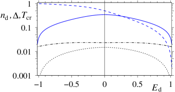
Figure 1: (colour online) The mean-field critical temperature $T_{cr}$ for a 2D EFKM at half-filling (n=1) with $U=1$ and the perturbation $t^{\prime}=-0.045$ (dotted line) or $V_{2}=0.15$ (dashed-dotted line). Solid and dashed lines show the unperturbed values of $\Delta$ and $n_{d}$ at $T=0$. The BEC scenario is realised as long as $T_{cr}$ is much smaller than crossover temperature $T_{*}$, which implies also $T_{cr}\ll U\Delta$.

At $H>0$, the phase transition is replaced by a smooth crossover, with $\cos\kappa$ asymptotically vanishing at high temperatures:

$$\cos\kappa\approx\frac{H}{2T-J}\,,\,\,\,\,\,T\gg J,H.$$ (98)

(note the similarity to the Curie–Weiss law). More generally (but still to leading order in $\delta{\cal H}$), $\cos\kappa$ throughout the $T\ll T_{*}$ range solves the equation

$$I_{0}\left(\frac{J\cos\kappa+H}{T}\right)\cos\kappa=I_{1}\left(\frac{J\cos\kappa+H}{T}\right)\,,$$ (99)

and should be found numerically (see Fig. 2 a).

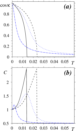
Figure 2: (colour online) Mean-field temperature dependence of $\cos\kappa$ (a) and specific heat (b) for a 2D EFKM with $U=1$ and $E_{d}=0.2$ at $n=1$ in the low-temperature regime. Solid and dashed lines correspond, respectively, to $t^{\prime}=-0.045$ ($T_{cr}\approx 0.014$) and $V_{2}=0.15$ ($T_{cr}\approx 0.024$). Dashed-dotted line corresponds to $V_{0}=-0.008$, and the dotted one to combined $t^{\prime}=-0.045$ and $V_{1}=-0.04$; from Eq. (94) one finds that for both of the latter two cases $H\approx 0.005$.

At low temperatures, $T\stackrel{{\scriptstyle<}}{{\sim}}T_{cr}$, and for $n=1$ (when the excitonic gap is present at the chemical potential), the contribution of fermionic degrees of freedom to entropy is exponentially small and can be neglected. Thus the entropy can be evaluated as $S=\log Z_{0}$ [see Eq. (96)], and the specific heat as $C=T\partial S/\partial T$. Using also Eq. (99), we find

$$C=-(J\cos\kappa+H)\frac{\partial\cos\kappa}{\partial T}+\frac{1}{2}\,.$$ (100)

At $H=0$, it suffers a negative jump of $\Delta C=-2$ at $T_{cr}$, whereas at $H>0$ and at temperatures $T\gg J,H$,

$$C\approx\frac{4TH^{2}}{(2T-J)^{3}}+\frac{1}{2}\,.$$ (101)

Numerical results for $C$ are shown in Fig. 2 b. The finite value of $C=1$ obtained at $T\rightarrow 0$ is an expected artefact of treating the $\phi$ and $\beta$ degrees of freedom classically. This value includes a $T$-independent (at $T\ll T_{*}$) contribution of $1/2$, originating from the small fluctuations of $\beta$, see Eq. (97). Taking into account small fluctuations of other classical degrees of freedom, which were assumed frozen [such as $\theta_{i}$ and $\gamma_{i}$ in Eq.(52)] will yield additional constant terms in the specific heat. On the other hand, treating all the degrees of freedom as quantum would not affect the value of $C$ at higher $T$, whereas at $T\rightarrow 0$ one would obtain the correct result, $C\rightarrow 0$. Obviously, a proper description in the latter regime should be based on the analysis of the low-energy, long-wavelength excitations (cf. Ref. prb12, ), rather than on a single-site approach as considered presently.

The numerical results shown in Fig. 2 were obtained as outlined above. First, the $T=0$ mean-field equations in the absence of $\delta{\cal H}$ were solved, producing the values of $\Delta$ and $n_{c,d}$ (see Fig. 1). These are substituted into the leading-order Eq. (99), yielding $\cos\kappa$ as a function of temperature (Fig. 2 a), and Eq. (100) then gives the specific heat (Fig. 2 b).

A more exact solution to the mean-field equations would require taking into account the subleading terms in powers of $\delta{\cal H}$, which in turn depend on $\cos\kappa$ both directly and self-consistently. However, such treatment is unwarranted here, in view of the obvious limitations of our approach at low $T$. In reality, the results obtained in this section are in any case only as good as a single-site description of an XY model in the low-temperature and critical regions would be (note also that the competitionFarkasovsky08 ; prb12 ; Batista02 between different phases at $T=0$ implies that the system is frustrated). In other words, they have a rough qualitative validity, missing a number of important features and strongly overestimating the stability of the ordered phase (and the value of $T_{cr}$).

Indeed, for the values of $U$ and $E_{d}$ used in Fig. 2, the analysisprb12 of low-energy spectra at $T=0$ gives the minimal absolute value of $t^{\prime}$ required to stabilised a uniform ordered phase as $|t^{\prime}_{cr}|\approx 0.04$. Hence we estimate that for $t^{\prime}=0.045$, which barely exceeds this, the actual value of $T_{cr}$ should be at least an order of magnitude smaller than $T_{cr}\approx 0.014$ shown in Fig. 2. The critical values of hybridisationsprb12 , $V_{0,cr}\approx-0.096$ and $V_{2,cr}\approx 0.21$ are greater than those used in Fig. 2, implying that in reality the ordering transition (which perhaps also takes place at a much lower temperature) is a transition into a competing charge-ordered state, and not into the uniform phase.

Physically, the reason for these inaccuracies is that in this regime an important rôle is played by the low-energy, long-wavelength collective excitationsprb12 (phase mode, as opposed to the amplitude mode discussed in Sec. VII.2 below), which cannot be treated adequately within a single-site approach. Furthermore, the actual behaviour may depend on the dimensionality of the system (as it does for the XY model, with 2D being a special case due to the possibility of vertex formationKosterlitz ), which is also overlooked in a single-site treatment. Noting that these shortcomings are shared by the available descriptions of the EFKM ordering transition, including Refs. Apinyan, ; condEFKM, , we omit further discussion of the literature.

However, we expect that these complications are restricted to the low-temperature range of $T\stackrel{{\scriptstyle<}}{{\sim}}T_{cr}$, whereas at higher $T$ (where short-range fluctuations become more prominent) one can hope to obtain a more faithful picture.

VI PHASE-DISORDERED EXCITONIC INSULATOR AND THE HIGH-TEMPERATURE CROSSOVER

Presently, we will consider the high-temperature regime of a fully phase-disordered excitonic insulator at $T\gg T_{cr}$. In this case, $\cos\kappa\rightarrow 0$ [see Eq. (98)] and therefore the perturbation $\delta{\cal H}$ vanishes on average, $\langle\delta{\cal H}\rangle_{T}=0$ (the latter equality holds to leading order in $T_{cr}/T$ and becomes exact in the case where $V_{0}=V_{1}=0$). Hence, formally $\delta{\cal H}$ does not affect the virtual-crystal Hamiltonian (13), nor indeed any quantity arising in our single-site mean-field description. While this writer believes that physically the perturbation is nevertheless essential for the validity of the qualitative scenario presented here, this is not the place for an in-depth discussion of this potentially controversial issue. Very briefly, we expect that the actual physical situation is reminiscent of that at $T=0$, when a finite, but small, value of $t^{\prime}$ or $V_{0,1,2}$ in Eq. (3) is requiredprb12 ; Farkasovsky08 to stabilise the state with a uniform value of $\Delta>0$ and a uniform $\phi$, yet once such a state is stable, the higher-energy properties of the mean-field solution (such as the magnitude of $\Delta$) to leading order do not depend on the perturbation. The difference here is that in the case of disordered $\phi$ the actual phase transition at the critical value of a perturbation parameterprb12 ; Farkasovsky08 (found to take place at $T=0$) should be replaced by a smooth crossover (where the value of $\Delta>0$ saturates once the perturbation strength exceeds a certain characteristic scale), since the system does not undergo a symmetry change.

We further note that even if the perturbation is not sufficiently strong to stabilise a uniform ordered excitonic insulator at $T=0$ and additional charge ordering appears at low temperatures (i.e., if the value of the corresponding perturbation parameter is less than the critical one), the analysis in this section is still likely to be relevant for the behaviour of the system at higher $T$, when both phase and charge orders melt. While this issue merits further study, it also falls beyond the scope of this work.

As we already mentioned in the Introduction, the phase-disordered excitonic insulator state does not break any symmetry, and therefore increasing temperature further should result in a decrease of $\Delta=\frac{1}{2}\langle\cos 2\theta_{3}\cos\theta_{1}\sin\beta\rangle_{T}$ [see Eq. (81)] via a smooth crossover. We are not specifically interested in the situation where the average value of $\theta_{1}$ approaches $0$ [corresponding to a band insulator without mixed valence, see Eqs. (82–83)] or $\pi/2$ (this corresponds to the high-temperature limit of the two equally populated bands and $\Delta\rightarrow 0$, see below). Elsewhere, weak or moderate fluctuations of $\theta_{1}$ around its average value do not affect the average values of $\Delta$ or $n_{d}$ and add little to the qualitative picture. Treating these fluctuations would also necessitate a straightforward but cumbersome calculation, as one cannot use a simpler formula, Eq. (58). Therefore, we will treat the angles $\theta_{1}$ and $\theta_{3}$ as frozen at their virtual-crystal values $\theta_{i}^{(0)}$. Fluctuations of the angle $\beta$, on the contrary, can affect the average value of $\Delta$, decreasing it when the average $\beta$ is close to $\pi/2$ and increasing $\Delta$ whenever the end points $0$ or $\pi$ are approached.

We also assume that the values of phases $\gamma_{i}$ in Eq. (53) are still frozen at $\gamma_{i}=0$; the effect of fluctuations of $\gamma_{i}$ will be discussed in Sec. VI.1. Then, the energy cost of a single-site fluctuation of the angle $\beta$ can be deduced from Eq. (138) as

$$\delta E(\beta) = 4l_{c}\sin^{2}\frac{\beta-\beta_{0}}{4}+2l_{\Delta}\sin\frac{\beta-\beta_{0}}{2}+$$

$$+\frac{E_{d}}{2}\sqrt{n^{2}-4\mathfrak{n}^{(0)}_{\mathfrak{d}}}\left(\cos\beta^{(0)}-\cos\beta\right)\,.$$

By construction, the value of $\delta E$ vanishes at $\beta=\beta^{(0)}$ (unperturbed virtual crystal). The quantities $l_{c}$ and $l_{\Delta}$ obey the self-consistency conditions,

$$\!\!\!l_{c} \!\!\!= \!\!\!\int_{0}^{\pi}\!\!\!\left(-l^{(0)}_{\Delta}\sin\frac{\beta-\beta^{(0)}}{2}+l_{c}^{(0)}\cos\frac{\beta-\beta^{(0)}}{2}\right)w(\beta)\sin\beta d\beta\,,$$

$$\!\!\!l_{\Delta} \!\!\!= \!\!\!\int_{0}^{\pi}\!\!\!\left(-l^{(0)}_{d}\sin\frac{\beta-\beta^{(0)}}{2}+l_{\Delta}^{(0)}\cos\frac{\beta-\beta^{(0)}}{2}\right)w(\beta)\sin\beta d\beta\,,$$

[see Appendix C, Eqs. (144–145)], with the values of $l^{(0)}_{c,d,\Delta}$ given by Eqs. (91), and

$$w(\beta)=\frac{1}{Q}\,{\rm e}^{-\delta E(\beta)/T}\,,\,\,\,Q=\int_{0}^{\pi}{\rm e}^{-\delta E(\beta)/T}\sin\beta d\beta\,.$$ (105)

Here the integration measure, $\sin\beta d\beta$, again comes from Eq. (76).

As the temperature is lowered toward $T_{cr}$, the fluctuations of $\beta$ become small, and one can expand Eq. (VI) in powers of $\delta\beta=\beta-\beta^{(0)}$. At the same time, the quantities $l_{c}$ and $l_{\Delta}$ approach their respective virtual-crystal values, $l_{c}^{(0)}$ and $l_{\Delta}^{(0)}$. Using also Eq. (95), we find for this low-$T$ region of the phase-disordered state

$$\delta E(\delta\beta)\approx\frac{1}{4}\left[l_{c}^{(0)}+E_{d}(n^{(0)}_{c}-n^{(0)}_{d})\right](\delta\beta)^{2}\,,$$ (106)

matching the last term in Eq. (90).

For all temperatures above $T_{cr}$, we can now use Eqs. (VI) and (105) to explicitly write Eqs. (88–89) as

$$\!\!\!\!\!\!\!\!\langle\delta\Delta\rangle_{T}=\frac{1}{2}\sqrt{n^{2}-4\mathfrak{n}^{(0)}_{\mathfrak{d}}}\int_{0}^{\pi}(sin\beta-\sin\beta^{(0)})w(\beta)\sin\beta d\beta\,,$$

(107)

$$\!\!\!\!\!\!\!\!\langle\delta n_{d}\rangle_{T}=\frac{1}{2}\sqrt{n^{2}-4\mathfrak{n}^{(0)}_{\mathfrak{d}}}\int_{0}^{\pi}(\cos\beta^{(0)}-\cos\beta)w(\beta)\sin\beta d\beta\,.$$

(108)

Standard deviations of $\Delta$ and $n_{d}$ from their average values,

$$\sigma_{\Delta} = \left[\langle\left(\delta\Delta-\langle\delta\Delta\rangle_{T}\right)^{2}\rangle_{T}\right]^{1/2}\,,$$ (109)

$$\sigma_{d} = \left[\langle\left(\delta n_{d}-\langle\delta n_{d}\rangle_{T}\right)^{2}\rangle_{T}\right]^{1/2}\,,$$ (110)

can be evaluated in a similar way. The mean-field scheme is closed by substituting (107–108) into Eqs. (25). The four resultant self-consistency equations [including also Eqs. (LABEL:eq:dlcT–LABEL:eq:dldeltaT)] are readily solved numerically.

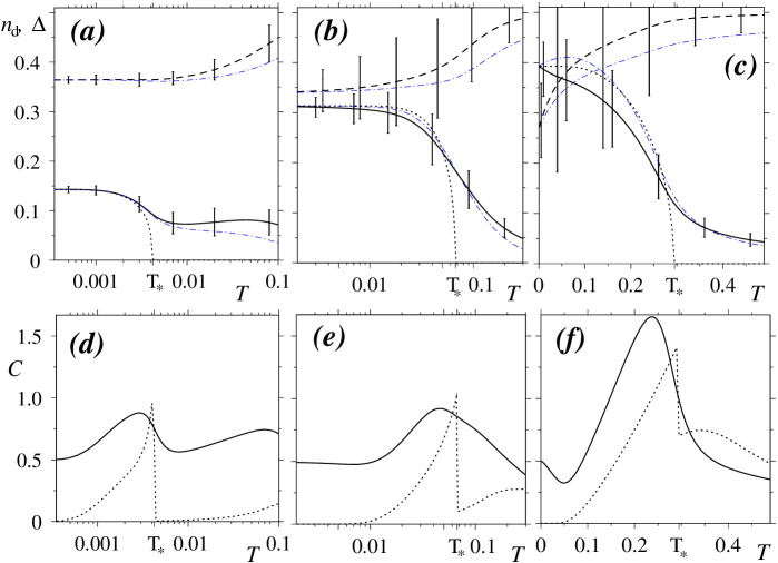
Figure 3: (colour online) Single-site mean-field solution for a 2D EFKM at $n=1$ in the phase-disordered region, $T>T_{cr}$, for $E_{d}=0.2$ and $U=0.5$ (panels a,d), $U=1$ (b,e), and $U=2$ (c,f). In panels a,b,c, the solid and dashed lines show the values of $\Delta$ and $n_{d}$, with the error bars corresponding to the standard deviations. The dashed-dotted lines represent the virtual-crystal contributions $\Delta^{(0)}$ and $n_{d}^{(0)}$, whereas the dotted lines show the Hartree–Fock solution for $\Delta$ which neglects the effect of thermal fluctuations on-site. In d,e,f, solid lines show the specific heat $C$ obtained for the full mean-field solution, whereas the dotted lines correspond to neglecting the thermal fluctuations.

Typical results, obtained for a two-dimensional system at $n=1$ are shown in Fig. 3. Since the ordering transition temperature is determined by the parameters of the perturbation $\delta{\cal H}$ (see Sec. V) and, at least within the present approach, can be arbitrarily small, we may carry out our computation for the phase-disordered state at any finite $T$ while assuming $T\gg T_{cr}$. The three values of $U$ used in Fig. 3 correspond to the cases of weak, intermediate, and strong coupling. The latter terminology refers not to the ratio between the crossover temperature $T_{*}$ and $T_{cr}$, but rather to the properties of the uniform mean-field solution of the pure $FKM$ at $T\rightarrow 0$, specifically to the value of the double occupancy on-site $\mathfrak{n}_{\mathfrak{d}}^{(0)}$ [Eq. (41)]. For $U=0.5$, $U=1$, and $U=2$ we obtain, respectively, $\mathfrak{n}_{\mathfrak{d}}^{(0)}\approx 0.21$, $0.13$, and $0.04$ in the limit of low $T$.

Neglecting thermal fluctuations of the OSDMHFcalc , one obtains a purely Hartree–Fock result for $\Delta(T)$, which in Figs. 3 a,b,c is represented by the dotted line. It incorrectly predicts a second-order phase transition at a certain temperature, which we will instead identify as the crossover temperature $T_{*}$. We find $T_{*}\approx 0.0042$ for $U=0.5$, $T_{*}\approx 0.067$ for $U=1$, and $T_{*}\approx 0.29$ for $U=2$. As expected, the value of the indirect gap $G$ at $T=0$ [$G\approx.00525$, $0.102$, and $0.647$, respectively, see Eq. (18)] yields a correct order-of-magnitude estimate of $T_{*}$, although it is worth noting that the fit worsens with increasing $U$. The latter is due to the fact that for larger $U$, the dominant contribution to the temperature dependence of energy comes not from the smearing of the Fermi distribution and the resultant particle-hole excitations across the gap, but rather from the changes of the average interaction energy per site, $U\mathfrak{n}_{\mathfrak{d}}=U\mathfrak{n}_{\mathfrak{d}}^{(0)}=U(n_{c}^{(0)}n_{d}^{(0)}-|\Delta^{(0)}|^{2})$. Indeed, for $U=1$ and $U=2$ the quantity

$$\langle\Delta E_{int}\rangle_{F}\sim U\left(\mathfrak{n}_{\mathfrak{d}}^{(0)}(T_{*})-\mathfrak{n}_{\mathfrak{d}}^{(0)}(0)\right)\,,$$ (111)

(the fluctuation-induced increase of the interaction energy from $T=0$ to $T=T_{*}$) gives a perfect estimate for $T_{*}$. On the other hand, it is actually negative for the weakly interacting case of $U=0.5$, where the net energy change is dominated by the effects of Fermi distribution smearing, and hence the single-particle gap $G$ yields a rather accurate estimate for $T_{*}$.

The values of $\Delta(T)$ and $n_{d}(T)$, obtained within our single-site mean-field approach, are illustrated by the solid and dashed lines, respectively, with the value of $\Delta(T)$ showing a smooth downturn in a broad region around $T_{*}$. In the $U=0.5$ case (Fig. 3 a), this is followed by an upturn, due to the increasing thermal fluctuations. Since the contribution of the small-$\Delta$ region is suppressed by the factor $\sin\beta$ in the measure [see Eq. (107)], these lead to the overall increase in $\Delta$. Indeed, in this region we see the increase of both the standard deviation, Eq. (109) (shown by the error bars), and of the difference $\langle\delta\Delta\rangle_{T}$ between the net $\Delta$ and its virtual-crystal part, $\Delta^{(0)}$, represented by the dashed-dotted line. Then, the value of $\Delta(T)$ passes through a broad maximum and begins its decrease to a higher-temperature mean-field solution, where both orbitals are equally populated [note that the monotonously increasing $n_{d}(T)$ is now approaching $1/2$] while $\Delta$ vanishes (whereby $\mathfrak{n}_{\mathfrak{d}}$ will reach its maximal value of $1/4$). This regime is formally possible only at $T{>}E_{d}$. Indeed, in the absence of $\Delta$, there are two unhybridised Hartree bands, dispersive and localised, and if these are equally populated the energy difference between their respective centres equals $E_{d}$; on the other hand, the two band occupancies can approach each other only when the temperature is large in comparison with this energy difference. Due to suppression of the fluctuations of $\Delta$, this configuration minimises the free energy at sufficiently high $T$.

Yet, it is clear that this “high-temperature limit” with $\Delta\rightarrow 0$ and $\sigma_{\Delta}\rightarrow 0$ is an artefact of our assumption that the fluctuations of $\theta_{i}$ can be omitted. Indeed, we observe that the case of $n_{c}=n_{d}$ and $\Delta=0$ corresponds to $\theta^{(0)}_{1}=\pi/2$ [see Eqs. (55) and (78)]. Since this is an endpoint of the variation range for $\theta_{1}$, the thermal fluctuations of this parameter will be asymmetric and will shift its average to lower values, increasing the difference $n_{c}-n_{d}$ and the fluctuations (and hence the average value) of $\Delta$. Moreover, an additional factor of $\cos^{2}\theta_{1}$ in the phase-space measure, Eq. (76), which reduces the relative contribution of the region near $\theta_{1}=\pi/2$ to the partition function, guarantees that the fluctuations of $\theta_{1}$ will be large, once $T$ becomes comparable to the energy scale associated with such fluctuations (which should be the largest of $E_{d}$ and $U$, possibly with a prefactor). Thus, we expect that the value of $\Delta(T)$ passes through a minimum at $T\stackrel{{\scriptstyle<}}{{\sim}}{\rm max}(E_{d},U)$ and begins to increase due to an overall increase of the thermal fluctuations at higher $T$. However, as explained in Sec.VI.1 below, this region is in any case out of reach for us, at least within the present version of our mean-field approach.

Interestingly, the increase of $n_{d}(T)$ and decrease of $\Delta(T)$ at $T<T_{*}$ lead to the value of $\mathfrak{n}_{\mathfrak{d}}^{(0)}(T_{*})$ being about the same, $\mathfrak{n}_{\mathfrak{d}}^{(0)}=0.21\pm 0.01$, in all three cases of $U=0.5$, $U=1$, and $U=2$. At $T>T_{*}$, the intermediate region of increasing $\Delta(T)$ is absent at higher $U$ (Fig. 3 b,c), for the following two reasons: (i) the corresponding values of $T$ are much larger, due to higher $T_{*}$, and therefore closer to the high-temperature regime, where the present calculation predicts a strong decrease of $\Delta$ (see the discussion above); (ii) the value of $\Delta$ is larger, therefore thermal fluctuations are nearly symmetric (the $\beta=0$ point is far away), and their contribution $\langle\delta\Delta\rangle_{T}$ to the net value of $\Delta$ is much smaller than in the low-energy case (and actually changes sign in the region above $T_{*}$). We note, however, that our results for higher $U$ (especially for $U=2$) become quantitatively unreliable in this region due to strong fluctuations of $\gamma_{i}$ (see Sec. VI.1 below).

The specific heat is calculated as $C=\partial\langle E\rangle_{T}/\partial T$. Here, the average energy per site,

$$\langle E\rangle_{T} = \langle{\cal H}\rangle_{F}+\langle\delta E\rangle_{T}=-l_{c}^{(0)}+E_{d}n_{d}^{(0)}+Un_{c}^{(0)}n_{d}^{(0)}-$$ (112)

$$-U(\Delta^{(0)})^{2}+\int_{0}^{\pi}\delta E(\beta)w(\beta)\sin\beta d\beta$$

[see Eqs. (91)], is the sum of the virtual-crystal contribution and the average fluctuation energy $\langle\delta E\rangle_{T}$. The calculated values of $C$ (solid lines in Fig. 3 d,e,f ) approach $0.5$ in the low-temperature limit (corresponding to the presence of one classical degree of freedom, $\beta$, and, in the case of Fig. 3 e, to the higher-$T$ part of Fig. 2 b), show a broad maximum in the crossover region $T\sim T_{*}$, and decrease at high temperatures [mirroring the decrease of $\Delta(T)$]. In the weakly interacting case of Fig. 3 d, the initial increase following the peak at $T\sim T_{*}$ corresponds to increasing $\Delta(T)$ in this region (see above). The dotted lines represent the Hartree–Fock resultsHFcalc (as described above for Fig. 3 a,b,c), including only the contributions from fermionic degrees of freedom and from the temperature dependence of the Hartree–Fock values of $\Delta$ and $n_{d}$. As expected, there is a negative jump at $T=T_{*}$, an artefact of neglecting the thermal fluctuations of the OSDM. It appears possible that the low-temperature limiting value $C\rightarrow 0.5$ is again an artefact of the classical treatment of the fluctuations of $\beta$ and a proper quantum treatment would yield $C\rightarrow 0$ at $T\rightarrow 0$ both for $T\ll T_{cr}$ (see Sec. V) and for the phase-disordered case of $T\gg T_{cr}\rightarrow 0$ (but certainly not for $T\sim T_{cr}$). At all events, the classical description of $\beta$ becomes more adequate with increasing $T$, and should be appropriate for most of the temperature range in Fig. 3 (where the relevant scale is that of $T_{*}$).

Finally, we are now in a position to clarify the importance of the self-consistency conditions (LABEL:eq:dlcT–LABEL:eq:dldeltaT). As exemplified in Fig. 4, the self-consistent renormalisation $\delta l_{c,\Delta}=l_{c,\Delta}-l_{c,\Delta}^{(0)}$ of the quantities $l_{c,\Delta}$ is rather small, its relative size increases moderately in the high-temperature region well above $T_{*}$. Importantly, if the self-consistency conditions (LABEL:eq:dlcT–LABEL:eq:dldeltaT) are omitted altogether, and one solves only two mean-field equations (25) for $n_{d}$ and $\Delta$ (substituting for $l_{c,\Delta}$ the values of $l_{c,\Delta}^{(0)}$, calculated for the same $n_{d}$ and $\Delta$), this leads to a small shift in the resultant mean-field solution, $n_{d}(T)$ and $\Delta(T)$. This small change, which peaks in the region of $T\sim T_{*}$, appears negligible for all practical purposes.

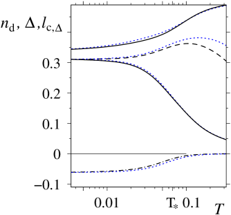
Figure 4: (colour online) The effect of self-consistent renormalisation of $l_{c,\Delta}$ on the mean-field solution. Dashed and dashed-dotted lines show, respectively, the self-consistent values of $l_{c}$ and $l_{\Delta}$ for a half-filled 2D EFKM with $U=1$ and $E_{d}=0.2$. The adjacent dotted lines show the unrenormalised virtual-crystal terms $l_{c,\Delta}^{(0)}$ [Eqs. (91)] calculated for the same self-consistent solution. The upper and lower solid lines show the self-consistent values of $n_{d}$ and $\Delta$ (same data as in Fig. 3 b), whereas the adjacent dotted lines correspond to the case where only two mean-field equations (25) are solved and the resultant unrenormalised $l_{c,\Delta}^{(0)}$ are substituted for $l_{c,\Delta}$.

It seems reasonable to expect that this unimportance of Eqs. (LABEL:eq:dlcT–LABEL:eq:dldeltaT) is a general property. While presently we had no difficulty carrying out the full self-consistent calculation, this would have been problematic had we included also the fluctuations of $\theta_{i}$ (see Sec. III for discussion). However, if the error introduced by substituting $l_{c,\Delta}^{(0)}$ in place of $l_{c,\Delta}$ is indeed insignificant, this would justify the use of a simpler Eq. (59) in place of a difficult Eq.(57).

To summarise, our single-site mean-field approach yields a physically transparent description of the phase-disordered state of the EFKM above the low-temperature ordering transition. This includes, at least for the case of weak to moderate interaction strength, the crossover region of $T\sim T_{*}$ (see Sec. VI.1 regarding larger values of $U$). It appears that previously such a description has been lacking, at least in the context of the EFKM. Further discussion of results obtained in this section will follow in Secs. VII and VIII.

VI.1 Validity of the Hartree-Fock approximation for the wave functions

The quantities $\gamma_{i}$ are additional phase variables of the SU(4) rotation (see Appendix B), which affect the wave function $|\tilde{\Psi}\rangle$ [Eqs. (52–53)], but not the corresponding OSDM [Eqs. (69) and (78)]. When either $\gamma_{1}$ or $\gamma_{3}$ differs from zero, an electron hopping to or from the central site acquires an additional phase which depends on the specific quantum state concerned (at the central site). Similarly, $2\gamma_{2}$ is the phase difference between the two singly occupied states which diagonalise the OSDM at the central site, and it affects both the phase carried away by a hopping electron and the hopping probability. Strong fluctuations of $\gamma_{i}$ would suggest a possibility of non-trivial phase-related phenomena, such as strongly fluctuating flux through a plaquette.

Importantly, the fluctuations of $\gamma_{i}$ cannot be incorporated into our self-consistent scheme, which relies on the underlying virtual crystal [Eq. (13)] and hence, on the corresponding Hartree–Fock wavefunctions $|\Psi\rangle$. The latter correspond to all $\gamma_{i}$ being equal to zero everywhere, and there is apparently no way to include the fluctuations of $\gamma_{i}$ by merely renormalising the parameters of the virtual crystal (and hence of $|\Psi\rangle$), as we did with the fluctuations of $\beta$ above, and with fluctuations of $\varphi$ in Sec. V [or as can be done with the fluctuations of $\theta_{1,3}$ under restriction (83)].

On the other hand, there is no difficulty in calculating the energy cost of a local fluctuation of both $\beta$ and $\gamma_{i}$ at site 0, provided that all $\gamma_{i}$ vanish elsewhere. In addition to $\delta E(\beta)$ [Eq. (VI)], the energy of such a fluctuation acquires another term, $\delta E_{\gamma}(\beta,\gamma_{1},\gamma_{2},\gamma_{3})$, given by Eq. (146). One can proceed one step further and calculate the average value of $\cos\gamma_{i}$ under such fluctuations as

$$\!\!\!\!\!\!\langle\cos\gamma_{i}\rangle_{T}=\int_{0}^{\pi}\!\!\sin\beta d\beta\int_{0}^{2\pi}\!\!d\gamma_{1}\int_{-\pi/2}^{\pi/2}\!\!d\gamma_{2}\int_{0}^{2\pi}\!\!d\gamma_{3}\tilde{w}\cos\gamma_{i}\,,$$

(113)

$$\!\!\!\!\!\!\tilde{w}(\beta,\gamma_{1},\gamma_{2},\gamma_{3})=\frac{1}{\tilde{Q}}\,{\rm e}^{-[\delta E(\beta)+\delta E_{\gamma}(\beta,\gamma_{1},\gamma_{2},\gamma_{3})]/T}\,,$$

$$\!\!\!\!\!\!\tilde{Q}=\int_{0}^{\pi}\!\!\sin\beta d\beta\int_{0}^{2\pi}\!\!d\gamma_{1}\int_{-\pi/2}^{\pi/2}\!\!d\gamma_{2}\int_{0}^{2\pi}\!\!d\gamma_{3}\tilde{w}(\beta,\gamma_{1},\gamma_{2},\gamma_{3})\,.$$

Figure 5: Thermal fluctuations of phases $\gamma_{i}$ for a 2D EFKM at $n=1$, for $E_{d}=0.2$ and $U=0.5$ (a), $U=1$ (b), and $U=2$ (c). Solid, dashed, and dotted lines show $\langle\cos\gamma_{i}\rangle_{T}$ for $i=1,2$ and $3$, respectively. Standard deviation is about $1-\langle\cos\gamma_{i}\rangle_{T}$ in all cases.

In Fig. 5, we plot the three quantities $\langle\cos\gamma_{i}\rangle_{T}$ for the three cases considered in Fig. 3 and corresponding to weak, moderate, and strong interaction $U$. While in the limit of $T\rightarrow 0$ all three values of $\gamma_{i}$ approach zero in all the three cases (attesting to the consistency of the underlying Hartree–Fock approximation at low $T$), the behaviour at increased temperatures shows a marked dependence on the interaction strength. In the weak-coupling case of Fig. 5 a, the values of $\langle\cos\gamma_{i}\rangle_{T}$ remain above $0.65$ throughout the entire range of the plot, including also the crossover region (at $T=T_{*}$ we find $\langle\cos\gamma_{i}\rangle_{T}\approx 0.986\pm 0.003$ for all $i$). With the fluctuations of $\gamma_{i}$ being either small or very moderate, we conclude that they indeed can be neglected, and the Hartree–Fock virtual-crystal treatment remains valid up to $T_{*}$ and beyond. At $U=1$ (see Fig. 5 b), the values of $\langle\cos\gamma_{i}\rangle_{T}$ at $T_{*}$ are $0.83$, $0.88$, and $0.73$ for $i=1,2$ and $3$, respectively, hence, we expect that the Hartree–Fock picture remains valid and qualitatively reliable up to $T_{*}$, but not much beyond that. Thus, one concludes that in these two cases the consistency of our mean-field approach at $T\stackrel{{\scriptstyle<}}{{\sim}}T_{*}$ is not in danger.

The situation is different for the strong-coupling case of $U=2$ (shown in Fig. 5 c), where the values of $\langle\cos\gamma_{i}\rangle_{T}$ at $T_{*}$ are approximately $0.34$, $0.68$, and $0.13$, which suggests that the fluctuations of $\gamma_{i}$ are no longer negligible in any sense. The Hartree–Fock description still remains applicable in the phase-disordered state, but at much lower temperatures: for example, at $T=0.03$ (and for $U=2$) we find $\langle\cos\gamma_{i}\rangle_{T}\approx 0.72$, $0.76$, and $0.31$ for $i=1,2$, and $3$. The strong fluctuations of $\langle\cos\gamma_{3}\rangle_{T}$ do not constitute an immediate cause for concern, as the phase $\gamma_{3}$ affects only the doubly-occupied component of the perturbed wave function (53), and the relative weight of this component at $T=0.03$ is still fairly small, with $\mathfrak{n}_{\mathfrak{d}}^{(0)}\approx 0.05$. We speculate that the overall behaviour suggested by Fig. 3 c, which is in line with the reliable results obtained for smaller $U$, is still probably correct, but this conjecture certainly lacks a solid justification.

Finally, we note that although the phases $\gamma_{i}$ do not directly affect the OSDM (including the fluctuating values of $n_{d}$ and $\Delta$), taking into account the fluctuations of $\gamma_{i}$ does modify the probability distribution for the angle $\beta$, and hence does affect the average values $\Delta(T)$ and $n_{d}(T)$ (as well as those of $l_{c,\Delta}$). In the region where our theory is applicable, this effect is not very strong, reaching up to 10% for $\Delta(T)$, and about 1 % for $n_{d}(T)$. The difference is most pronounced in the region where the fluctuations of $\Delta(T)$ are largest, thus falling well within the “error bars” on Fig. 3 a,b,c. Likewise, the relative change of the net $l_{c,\Delta}$ seldom exceeds 15% (whereas the values of $\delta l_{c,\Delta}$, see above, can become several times larger or smaller). Accordingly, when one substitutes $\tilde{w}$ given by Eq. (113) in place of $w$ in the Eqs. (107–108) of the self-consistent calculation and includes additional integration over $\gamma_{i}$, the resultant change of $n_{d}(T)$ and $\Delta(T)$ is within 10%, with no new features (we checked this for $U=1$ and $T{<}0.1$).

VII Excitonic insulators – experiment and theory

VII.1 Experimental situation: The case of ${\rm Ta_{2}NiSe_{5}}$

Experimentally, specific heat $C$ was measuredFu2017 in an excitonic insulator candidate ${\rm Ta_{2}NiSe_{5}}$. In this compound, a phase transition is observed at $T=326$ K, accompanied by a symmetry change and by a peak in the $C(T)$ dependence; below the transition, the (direct) interband gap has a flattened momentum dependenceWakisaka09 ; Seki14 , suggestive of an excitonic insulator. There is an ongoing discussion as to whether the transition is primarily of electronicMazza19 or latticeWatson19 origin, and it is clear that electronic and lattice degrees of freedom are interdependent. Since the (long-range) lattice strain fields are presumably coupled to the phase degree of freedom in the electronic insulator (our $\varphi_{i}$), one expects that this increases the energies of collective excitations in the low-$T$ ordered phase. This might in turn push the value of the ordering transition temperature $T_{cr}$ upwards, shrinking or obliterating the phase-disordered intermediate region $T_{cr}<T<T_{*}$, discussed in Sec. VI above.

In is generally considered as plausible that the featureFu2017 seen in $C(T)$ at $326$ K corresponds to this increased value of $T_{cr}$ (excitonic condensation); the transition is still second order, although modified (in comparison to the one discussed in Sec. V) by a strong involvement of the lattice. The apparent absence of hybridisation above the transitionWatson19 ; Lee19 suggests that there is no further high-temperature crossover (our $T_{*}$) located in that region. Mutatis mutandis, this is a BCS-type pictureLee19 , which is also consistent with the expectationSeki14 ; Sugimoto18 that the effective masses in the two bands are not very different. Yet, we note that a phase-disordered excitonic insulator with $T_{*}$ above $326$ K, while characterised by a small (fluctuating) hybridisation gap, on average would not violate the higher lattice symmetry; this opportunity, and the corresponding BEC behaviour, are discussed in Refs. Seki14, ; Sugimoto18, , which also identify the transition at $326$ K as the excitonic ordering temperature (our $T_{cr}$).

Another scenario would have the (lattice) transition at $326$ K accompany (and perhaps sharpen) the excitonic crossover [hence, $T_{*}\approx 326$ K, cf. the peak of $C(T)$ at $T\sim T_{*}$ in Fig. 3 d,e,f ], and the excitonic ordering take place at a lower $T_{cr}$; with the lattice symmetry breaking playing the role of “external field” $H$ in a corresponding XY model [cf. Eq. (94)], the transition at $T\sim T_{cr}$ and the associated jump in $C$ would both be smeared and perhaps difficult to pinpoint200K (cf. the dotted line in Fig. 2 b, and the discussion in Sec. V). This would constitute a pronounced excitonic BEC behaviour with a weak or moderate coupling to the lattice and $T_{*}/T_{cr}\gg 1$ or $T_{*}/T_{cr}\stackrel{{\scriptstyle>}}{{\sim}}1$. Note that (i) in principle, the existence of the condensate extends all the way up to $326$ K [cf. Eq. (98); in our theoretical analysis in Sec. VI, carried out for $T\gg T_{cr}$, this effect was neglected]; (ii) the latter is not sufficient to identify $326$ K as the excitonic BEC transition temperature $T_{cr}$; this is similar to magnetisation being induced by an external field in a ferromagnet above the Curie point.

Finally, if hybridisation is dominated by the lattice effects at all temperatures, with excitonic pairing providing a perturbative correction at low $T$, the system should not be termed an excitonic insulator. The experimental resultsLarkin17 ; Werderhausen18 , however, point to strong excitonic effects, which in turn affect the properties of phonons.

We note that the value of excitonic order parameter directly influences the electrostatic properties of the system. In the case of ${\rm Ta_{2}NiSe_{5}}$, the gap is direct, and uniform ($\vec{k}=0$) measurements of the appropriate electrostatic moment (possibly quadrupole rather than dipole one, in contrast to a simpler case considered in Refs.Portengen, ; Batista04, ; pssb13, ) and of the corresponding response should be performed in order to identify the correct scenario. Dynamical measurements might allow to distinguish between the lattice (slow) and excitonic (fast) contributions, as suggested also in Ref. Mazza19, . In addition, further assistance in assigning the value of $T_{cr}$ and (if distinct) of $T_{*}$ can be drawn from studying the spectra of phase and amplitude collective modes.

VII.2 Amplitude mode and amplitude susceptibility

The presence of a non-zero absolute value $\Delta$ of the on-site hybridisation implies the existence of a collective mode, corresponding to its oscillations. Presently, this subject receives much attention both in the framework of general interest in such “Higgs mode” in solid state physicsHiggs , and in a more narrow context of prospective excitonic insulators. Indeed, an important recent paperKogar2017 is devoted to experimental identification of the amplitude mode in the case of dichalcogenide ${\rm 1}T-{\rm TiSe}_{2}$; presence of such a mode was also reportedWerderhausen18 for ${\rm Ta_{2}NiSe_{5}}$, where its fingerprint is seen in the phonon dynamics. Therefore, it appears important to discuss the insight which can be gained from our present work in this regard.

If one neglects thermal fluctuations of the OSDM (including those of the phases $\varphi_{i}$; this is the “pure Hartree–Fock” case discussed above, corresponding to the dotted lines in Fig. 3), the spectrum $\omega_{\vec{q}}$ of higher-energy plasmon excitation can be calculated along the lines of Ref.prb12, . To zeroth order in $\delta{\cal H}$ and for the case of $\vec{q}=0$, the secular equation takes the formsecular :

$$\omega^{2}\left\{\left[J_{1}(\omega)\right]^{2}+\left(u^{2}-\omega^{2}\right)\left[J_{0}(\omega)\right]^{2}\right\}=0\,$$ (114)

[see Eq. (6)], where for $l=0,1$

$$J_{l}(\omega)=\frac{1}{N}\sum_{\vec{k}}\frac{\Delta_{\vec{k}}}{\Delta}\frac{\xi_{\vec{k}}^{l}}{u^{2}-\omega^{2}+\xi_{\vec{k}}^{2}}$$ (115)

[see Eqs. (16) and (22); upon converting the r. h. s. of Eq. (115) to an integral, principal value of the latter should be evaluated].

Eq. (114) is valid below the Hartree–Fock critical point $T_{*}$ and has two solutions. Of these, $\omega=0$ corresponds to the phase mode, vanishing in the unperturbed case of $\delta{\cal H}=0$ (for $T=0$, the perturbed case is investigated in detail in Ref. prb12, ). The other solution, which must correspond to the amplitude mode, lies above the direct gap $u=2U\Delta$, which means that it is likely to be strongly damped by the particle-hole excitations. Typical behaviour of $\omega^{2}(T)$ is plotted in Figs. 6 a,b with solid lines (left scale). As expected, it vanishes at $T\rightarrow T_{*}$.

For a relatively small $U=0.5$, the value of $\omega$ closely follows that of $u$ (see Fig. 6 a). We note that smaller $U$ results also in smaller values of $\Delta$ (cf. Fig. 3), leading to a strong overall decrease in $u=2U\Delta$. In this case, it appears that also away from $T_{*}$ the non-zero solution of Eq. (114) is strongly affected by a somewhat complex anomaly of $J_{0}$ [Eq. (115)], located at $u,\omega\rightarrow 0$. This is no longer the case for $U=1$ (see Fig. 6 b), where $\omega$ is found to exceed $u$ significantly.

Above $T_{*}$, the phase mode must disappear (as there is no corresponding symmetry breaking), whereas the amplitude mode is expected to recover to higher energies (see below). However, it can no longer be represented as a linear combination of particle-hole excitations and hence cannot be calculated within the approach of Ref. prb12, .

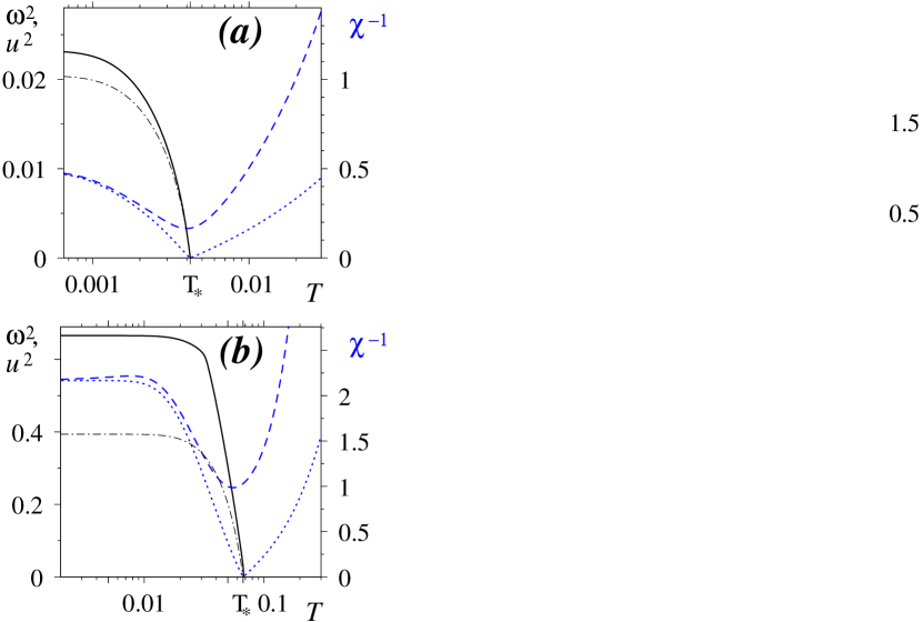
Figure 6: (colour online) Solid line (left scale) shows the amplitude mode energy squared for a half-filled 2D EFKM with $E_{d}=0.2$ and $U=0.5$ (a) or $U=1$ (b), calculated at $\vec{q}=0$ and in the absence of the thermal fluctuations of the density matrix [Hartree–Fock, see Eq. (114)]. The dashed-dotted line (left scale) represents $u^{2}$, square of the direct energy gap. Dashed and dotted lines (right scale) correspond to an inverse susceptibility, $1/\chi$. Dashed line includes the effect of thermal fluctuations of the OSDM.

It is unclear whether this approach can be extended to include the thermal fluctuations of the OSDM, and whether the time-independent treatment of these, as constructed in this paper, would be sufficient. At all events, the energy scale of the amplitude fluctuations can be deduced from the value of susceptibility $\chi=\partial\Delta/\partial{\mathfrak{F}}$ with respect to a fictitious external scalar field ${\mathfrak{F}}$, coupled to the absolute value of the hybridisation. If the amplitude mode is present, its energy squared, $\omega^{2}$, can be expected to be roughly proportional to $1/\chi$, with the unknown $T$-dependent coefficient affected by the quantisation of the fluctuations of $\Delta$ and by the precise form of the excitation wavefunction. In order to calculate $\chi$, one must add the term

$$\delta_{\mathfrak{F}}{\cal H}_{mf} = -\frac{1}{2}{\mathfrak{F}}\sum_{i}\left(c^{\dagger}_{i}\tilde{d}_{i}+\tilde{d}_{i}^{\dagger}c_{i}\right)=$$ (116)

$$= -\frac{1}{2}{\mathfrak{F}}\sum_{\vec{k}}\left(c^{\dagger}_{\vec{k}}{d}_{\vec{k}}+{d}_{\vec{k}}^{\dagger}c_{\vec{k}}\right)$$

[cf. Eq. (7)] to the mean-field (virtual-crystal) Hamiltoniansubstit , Eq. (13) [see also Eq. (9)], and

$$\delta_{\mathfrak{F}}E(\beta) = -{\mathfrak{F}}\left[\tilde{\Delta}(\beta)-\Delta^{(0)}\right]=$$ (117)

$$= -\frac{1}{2}{\mathfrak{F}}\sqrt{n^{2}-{\mathfrak{n}}_{\mathfrak{d}}}\left(\sin\beta-\sin\beta^{(0)}\right)$$

[see Eq. (81)] to the single-site fluctuation energy in the phase-disordered state, Eq. (VI). As before, our single-site approach dictates that the contribution of $\delta{\cal H}$ [Eq. (3)], vanishes in the phase-disordered regime above $T_{cr}$, hence, $\delta{\cal H}$ can be dropped altogether.

We first consider the purely Hartree–Fock case when the thermal fluctuations are neglectedHFcalc , which corresponds to the dotted lines in Figs. 6 a,b (right scale). The second-order phase transition is then located at $T=T_{*}$ (with $\Delta$ being the order parameter), and the behaviour of $\chi(T)$ conforms to a simple Landau theory. At $T<T_{*}$, the free energy $F$ as a function of $\Delta$ has a minimum at $\Delta=\Delta^{(0)}>0$, resulting in a finite $\chi$. The value of $\Delta^{(0)}$ decreases with temperature, and both $\Delta^{(0)}$ and $\partial^{2}F/\partial\Delta^{2}$ vanish at $T_{*}$, hence, $1/\chi$ vanishes [as does the actual value of $\omega^{2}$, available in this case from Eq. (114)]. Thereafter, $\Delta^{(0)}$ remains equal to zero, whereas the second derivative becomes finite, leading to a recovery of $1/\chi$.

When the thermal fluctuations of the OSDM are included, the average $\Delta$ remains finite at all temperatures. Accordingly, the zero of $1/\chi$ at $T=T_{*}$ is replaced by a broad minimum (see the dashed lines in Fig. 6). Note also a pronounced hardening of amplitude fluctuations at higher $T$, due to the increase of the corresponding derivative of $F$ (the increase of thermal fluctuations pushes the average $\Delta$ towards larger values, where the dependence of the energy on hybridisation amplitude is more sharp).

Note that both curves merge in the limit of low $T$. This illustrates the fact that, to leading order in $\delta{\cal H}$, the value of $\chi$ is unaffected by the phase ordering arising below $T_{cr}$. The effect of the exciton condensation on $\chi$ is therefore confined to a small correction (subleading term), which vanishes above $T_{cr}$.

In terms of collective excitation energies in the presence of thermal fluctuations, these results add up to a rather coherent qualitative picture. While the phase mode softens at the low-temperature ordering transition, $T=T_{cr}$, and is absent anywhere above $T_{cr}$, the amplitude mode is only weakly affected by the excitonic condensation taking place at $T_{cr}$. The phase-mode spectrum at $T<T_{cr}$ crucially dependsprb12 on the perturbation, Eq. (3), yet the latter to leading order does not affect the amplitude mode, yielding a small correctionsmallcorr only. At higher $T$, the amplitude mode energy shows a broad minimum in the crossover region, $T\approx T_{*}$, above which it increases to the values which are higher than those of the lower-temperature region, $T<T_{*}$. As to whether the amplitude excitation corresponds to an actual propagating mode or to a broadened resonance-type feature, this depends on the strength of damping and cannot be discussed here.

We are now in a position to compare these expectations to the experimental results for ${\rm 1}T-{\rm TiSe}_{2}$, reported in Ref. Kogar2017, , and to their suggested interpretation. The plasmon mode described there is identified as the amplitude mode of an excitonic insulator, whereas the phase mode is either absent or not detectable. When the temperature increases towards $T_{C}\approx 190K$, the amplitude mode energy gradually decreases toward that of the low-energy phonon and possibly vanishesfiniteq at $T=T_{C}$ (the error bars are relatively large). At higher temperatures it rebounds and becomes larger than in the low-$T$ region below $T_{C}$. The suggested interpretationKogar2017 is that $T_{C}$ corresponds to a phase transition, specifically – to exciton condensation. This implies the BCS (as opposed to BEC) scenario, and appears plausible indeed, especially assuming that the effective masses of the two bands are not too differentMonney2012 (the opposite situation would likely lead to the BEC physics).

However, positive identification of the excitonic condensate based on its excitation spectrum requires detecting a phase mode, which in this case would exist only below $T_{C}$, softening and vanishing at the transition point. As this mode was not observed, it appears possible that the excitonic transition, while lying low in energy, is pre-empted by a Peierls one.

We further note that the observed amplitude mode spectrum may also suggest another possibility, viz., that of the BEC scenario as discussed in this work. Then, the broad minimum of the mode energy around $T_{C}$ would correspond to the higher-temperature crossover (our $T_{*}$), and not to the excitonic condensation (which might or might not take place at a lower temperature $T_{cr}$, below which the phase-mode energy would increase sharply). The superlattice reflections observed below $T_{C}$ (see discussion in Ref. Kogar2017, ) would then be due to a structural change, perhaps with additional contribution from the stable exciton gas (as opposed to condensate), which arises at $T<T_{*}$ (see discussion in Sec. I). If the excitonic condensation temperature $T_{cr}$ is indeed below $T_{C}$, the former would again correspond to a smeared transition (see Sec. VII.1 above; in this situation, one does not expect the phase mode to completely disappear above $T_{cr}$, nor would its energy exactly vanish at $T_{cr}$).

Although the present discussion of the amplitude mode is clearly of a preliminary character, we expect that our conclusions are solid at the qualitative level. This applies both to the overall temperature dependence of the mode energy and to the need for further measurements in order to clarify the experimental situation reported in Ref. Kogar2017, .

VIII DISCUSSION AND OUTLOOK

Our mean-field treatment of the EFKM yields a physically transparent description of the excitonic insulator in a broad range of temperatures and fully supports the general expectations discussed in Sec. I. In particular, we were able to characterise the phase-disordered state, including the crossover region, $T\sim T_{*}$, and such a quantitative description appears to represent a new development in the general context of correlated electron systems with interaction-induced pairing in the BEC regime. While at the low-temperature region around the ordering transition (exciton condensation) the theory has at best a rough qualitative accuracy due to shortcomings expected of any single-site treatment at low $T$, there is ample reason to expect higher reliability at larger $T$, except in the high-temperature region for the case of strong interactions. We therefore suggest that these results provide a sound base for a more detailed description of the phase-disordered excitonic insulator, including susceptibilities and transport properties. Presently, our results lead to two conclusions, and we suggests that these should be checked for those compounds which are suggested as possible narrow-band (i.e., BEC rather than BCS) excitonic insulators.

First, in the phase-disordered state above the phase transition at $T_{cr}$ there exists a crossover temperature $T_{*}$, corresponding to a smooth decrease of the induced hybridisation $\Delta(T)$ and to an equally smooth peak in the specific heat $C(T)$. The order-of-magnitude estimate of $T_{*}$ is given by the value of indirect energy gap $G$ at $T=0$ [Eqs. (18) or (5)] (but see further discussion in Sec. VI). Second, while the value of $\Delta(T)$ above $T_{*}$ is smaller than below, it is still of the same order of magnitude (i.e., not small in absolute terms), and this situation persists until much higher temperatures. This is due to the thermal fluctuations of $\Delta$, which increase with $T$ and are naturally asymmetric (with $\Delta$ being defined as a positive quantity, its fluctuating value cannot dip below zero). In addition, the phase space where these fluctuations occur is built in such a way that the contribution of the small-$\Delta$ region is suppressed. Technically, this is represented by the factor $\sin\beta$ in the integration measure in Eq. (107) [or in a more general Eq. (67)] and may be interpreted as a reminder about the fact that while within this temperature region the phase $\phi$ of the induced hybridisation is completely disordered, it is still present as a physical variable. Indeed, had this not been the case, the measure of the fluctuations of $\Delta$ would correspond to O(1) rather than to SU(2), leading to a replacementphysicab18 $\sin\beta d\beta\rightarrow d\beta$. Above $T_{*}$, the value of $\Delta(T)$ initially continues to decrease with increasing $T$; it is expected to pass through a minimum (possibly at rather high temperatures, when $T$ becomes comparable to the bandstructure energy scales, viz., $T\stackrel{{\scriptstyle>}}{{\sim}}E_{d}$, see Sec. VI), which is followed by an increase driven by the increasing thermal fluctuations of the OSDM.

In recent years, both theoreticalcondEFKM and experimental studies of purported excitonic insulators have been enjoying a pronounced renaissance. In most compounds where the excitonic behaviour was suggested (with a likely exception of ${\rm Ta_{2}NiSe_{5}}$, see discussion in Sec. VII.1 and Refs. Fu2017, ; Wakisaka09, ; Seki14, ; Mazza19, ; Watson19, ; Lee19, ; Sugimoto18, ; Larkin17, ; Werderhausen18, ), it involves a narrow (or massive) band. These candidate BEC excitonic insulators include, in addition to the familiar samarium and thulium compoundsSmTm ; samariumth , a dichalcogenide semimetal1TTiSe2 ; Kogar2017 $1T$-TiSe₂, and also graphene multilayers at high magnetic fieldsgraphene . Recent theoretical and experimental contributions are typically focused on the ordered phase, or on the ordering transition (“exciton condensation”), although it appears possible that the features seen in some of the measurements actually correspond to the higher-temperature crossover ($T_{*}$ rather than $T_{cr}$, see Secs. VII.1 and VII.2), and are incorrectly attributed to $T_{cr}$. While the first experiments reporting observations of a disordered excitonic insulator above $T_{cr}$ are already availableMonney2012 ; aboveTcr , neither positive identification of this state nor a direct comparison to our theory are possible at this stage. Experimentally, the specific-heat measurements are still lacking for all compounds apart from ${\rm Ta_{2}NiSe_{5}}$, while the theory should be extended to clarify the role of other degrees of freedom (spin, lattice, and charge ordering), which are clearly importantcondEFKM at low $T$ and perhaps may significantly modify the system properties also at higher temperatures. Given the rapid development of the field, we expect a significant progress in the near future.

Importantly, we anticipate that the formalism, developed in Secs. III and IV, can be generalised to other systems with interaction-induced pairing. This includes both bulk systems (such as Kondo lattice and related models for the heavy-fermion systems) and lattice impurity models. While the latter are typically amenable to much more refined theoretical treatments, constructing an OSDM-based mean-field approach still can be expected to yield new insights into the properties of the method and possibly into those of the physical system as well.

Therefore, comments are in order concerning some aspects of the newly developed OSDM-based mean field formalism. Presently, we implemented it in Secs. V and VI in a rather truncated form, only for the half-filled ($n=1$) two-dimensional case and omitting fluctuations of the eigenvalues of the OSDM (parameters $\theta_{i}$) and (aside from a brief qualitative discussion in Sec. VI.1) those of the phases $\gamma_{i}$ [the three SU(4) phases which affect the wave function (53), corresponding to a single-site fluctuation]. The dimensionality of the system is hardly important at the mean-field level, and especially in the phase-disordered state, where the short- to medium-range correlations are expected to dominate. Regarding the value of $n$, it appears that studying a system with any carrier density (as long as it supports pairing) should not present a difficulty, at least in principle. The same apparently applies to treating the fluctuations of $\theta_{i}$ and $\gamma_{i}$ in the case of correlated impurity (Kondo, Anderson, etc.) problems. On the other hand, fully including fluctuations of $\gamma_{i}$ (or unrestricted fluctuations of $\theta_{3}$) in a bulk system would require going beyond the underlying Hartree–Fock approximation, and it is presently unclear whether and how this could be performed.

The question of including fluctuations of $\theta_{i}$ which preserve the Hartree–Fock condition, $\mathfrak{n}_{\mathfrak{d}}=n_{c}n_{d}-|\Delta|^{2}$ in the case of EFKM [see Eq. (83), valid at $n=1$], for a bulk system is more subtle. Strictly speaking, in this case the fluctuations of the OSDM on different sites are not mutually independent (see Sec. III), which precludes full self-consistency of a single-site mean-field approach. On the other hand, there is a good reason to expect that the correction introduced by this inter-dependency is small and can be neglected (see Sec. VI). In this case, such fluctuations can be treated in a cumbersome but straightforward way, using a reduced equation (59). Yet, we suspect that such a calculation might not prove worthwhile, as the weak to moderate symmetric fluctuations of $\theta_{i}$ about their respective virtual-crystal average values are unlikely to significantly affect the results in the region of interest, $T\stackrel{{\scriptstyle<}}{{\sim}}T_{*}$.

One might also view this issue in a rather more pedantic way: We set out to build an analogue of the Weiss-type mean-field theory for a system with itinerant carriers. Considering all possible single-site fluctuations, we found that there exists a subclass of these, which allows in principle for a full self-consistency of this approach. This subclass includes the fluctuations of the OSDM parameters $\beta$ and $\phi$ (and also $\gamma_{i}$), corresponding to $\hat{S}\hat{S}^{\dagger}=1$ (see Sec. III). Hence this technique may prove useful in analysing the physical systems where fluctuations of the transverse component of the density matrix are expected to play a rôle, including excitonic insulators, heavy-fermion systems, superconductors and perhaps also spin-polarised systems where the (on-site) transverse spin dynamics is important. As for the opposite case when the OSDM is fully diagonal, the need for a Weiss-type treatment there is doubtful, as such “longitudinal” problems are best addressed by more conventional means, including the analysis of plasmon spectra, etc.

Appendix A On-site fluctuations in a lattice Fermi gas

What follows is a rather obvious derivation, included here for completeness. Consider for simplicity a single-band ideal Fermi gas on a lattice, with an arbitrary dispersion law. Let $\hat{F}$ be an on-site operator of the form

$$\hat{F}=\frac{1}{N}\sum_{\vec{k}}F(\vec{k})\hat{n}_{\vec{k}}\,,$$ (118)

where $\hat{n}_{\vec{k}}=g^{\dagger}_{\vec{k}}g_{\vec{k}}$ is the occupancy, $g_{\vec{k}}$ are the fermion annihilation operators, and the summation is over the Brillouin zone. Our local operators $c^{\dagger}_{0}c_{0}$, $d^{\dagger}_{0}d_{0}$, or $c^{\dagger}_{0}d_{0}$, whose average values yield band occupancies or hybridisation (see Secs. II–III), all have the general form (118). In these cases, the function $F({\vec{k}})$ contains also the coefficients of transformation from the Hartree–Fock quasiparticle operators $f_{a,{\vec{k}}}$ to the original fermions $c_{\vec{k}}$, $d_{\vec{k}}$, see Eqs. (II–21). We find

$$\bar{F}\equiv\langle\hat{F}\rangle_{F}=\frac{1}{N}\sum_{\vec{k}}F(\vec{k}){n}_{\vec{k}}\,,$$

where $n_{\vec{k}}$ is the Fermi distribution function, and likewise

$$\langle{\delta F}^{2}\rangle_{F} = \langle(\hat{F})^{2}-\left(\bar{F}\right)^{2}\rangle_{F}=$$

$$= \frac{1}{N^{2}}\sum_{\vec{k},\vec{p}}F(\vec{k})F(\vec{p})\langle\hat{n}_{\vec{k}}\hat{n}_{\vec{p}}-n_{\vec{k}}n_{\vec{p}}\rangle_{F}.$$

Since the occupancies for different momenta are statistically independent, the non-zero contribution comes only from the $\vec{k}=\vec{p}$ terms [where one obtains the well-known formulaVolume5 for the occupancy fluctuation, $\langle(\delta n_{\vec{k}})^{2}\rangle_{F}=n_{\vec{k}}(1-n_{\vec{k}})$]. Thus,

$$\sqrt{\langle{\delta F}^{2}\rangle_{F}}=\left\{\frac{1}{N^{2}}\sum_{\vec{k}}[F(\vec{k})]^{2}n_{\vec{k}}(1-n_{\vec{k}})\right\}^{1/2}\propto\frac{1}{\sqrt{N}}\,,$$ (119)

and vanishes in the $N\rightarrow\infty$ limit. Generalisation for a two-band case and for higher-order local operators $\hat{F}$ is straightforward.

We emphasise that Eq. (119) applies to finite-temperature fluctuations in a canonical ensemble, and not to quantum-mechanical fluctuations of an observable in a given state $|\Psi\rangle$.

Appendix B On-site fluctuations of the many-body wave function

We re-write Eq.(30) as

$$|\Psi\rangle= \!\!\!\!\!\!A_{a}^{(0)}|a\rangle|\Phi_{a}(\Psi)\rangle+A_{b}^{(0)}|b\rangle|\Phi_{b}(\Psi)\rangle+$$ (120)

$$\!\!\!\!\!\!+A_{0}^{(0)}|0\rangle|\Phi_{0}(\Psi)\rangle+|A_{cd}^{(0)}|\cdot|ab\rangle|\Phi_{cd}(\Psi)\rangle\,,$$

where the states $|\Phi_{i}(\Psi)\rangle$ are orthonormal. In the last term, we introduced

$$|ab\rangle\equiv a^{\dagger}b^{\dagger}|0\rangle={\rm e}^{{\rm i}\varphi_{0}}|cd\rangle$$ (121)

[see Eqs. (LABEL:eq:A0subst–44)]. The state of the system is affected by the choice of the on-site states $|c\rangle$ and $|d\rangle$ relative to $|a\rangle$ and $|b\rangle$ [cf. Eqs (43– 44); this affects the values of $\rho_{11}$, $\rho_{22}$, and $\rho_{12}=\rho_{21}^{*}$ but not the eigenvalues of the OSDM, $\hat{\rho}$], and by varying the coefficients $A_{i}$ (which in turn changes the eigenvalues). The states $|\Phi_{i}\rangle$ relate only to the rest of the system and are unaffected by the on-site fluctuations.

The changes of $A_{i}$ are described by SU(4) transformations in the four-dimensional space of orthonormal vectors $|a\rangle|\Phi_{a}\rangle$, $|b\rangle|\Phi_{b}\rangle$, $|0\rangle|\Phi_{0}\rangle$, and $|ab\rangle|\Phi_{cd}\rangle$ (matrix equations that follow assume this order of basic vectors). While one could act with an SU(4) transformation ${\cal D}$ on the original state (120), it is more convenient to choose a fixed initial state, $|\psi_{0}\rangle=|ab\rangle|\Phi_{cd}(\Psi)\rangle$. As explained in Ref. physicab18, (see also Ref. Tilma2002, ), one can then use a reduced form $\tilde{{\cal D}}$ of the SU(4) transformation matrix, depending only on six Euler angles (instead of 15):

$$\!\!\!\!\!\tilde{\cal D}\!\!=\!\!\!\left(\!\!\!\begin{array}[]{cccc}{\rm e}^{{\rm i}(\alpha_{1}+\alpha_{2}+\alpha_{3})}\cos\frac{\theta_{1}}{2}\cos\theta_{2}\sin\theta_{3}&{\rm e}^{{\rm i}(\alpha_{1}-\alpha_{2}-\alpha_{3})}\sin\frac{\theta_{1}}{2}&{\rm e}^{{\rm i}(\alpha_{1}+\alpha_{2})}\cos\frac{\theta_{1}}{2}\sin\theta_{2}&{\rm e}^{{\rm i}(\alpha_{1}+\alpha_{2}+\alpha_{3})}\cos\frac{\theta_{1}}{2}\cos\theta_{2}\cos\theta_{3}\\ {}\hfil&{}\hfil&{}\hfil&{}\hfil\\ -{\rm e}^{{\rm i}(-\alpha_{1}+\alpha_{2}+\alpha_{3})}\sin\frac{\theta_{1}}{2}\cos\theta_{2}\sin\theta_{3}&{\rm e}^{-{\rm i}(\alpha_{1}+\alpha_{2}+\alpha_{3})}\cos\frac{\theta_{1}}{2}&-{\rm e}^{{\rm i}(-\alpha_{1}+\alpha_{2})}\sin\frac{\theta_{1}}{2}\sin\theta_{2}&-{\rm e}^{{\rm i}(-\alpha_{1}+\alpha_{2}+\alpha_{3})}\sin\frac{\theta_{1}}{2}\cos\theta_{2}\cos\theta_{3}\\ {}\hfil&{}\hfil&{}\hfil&{}\hfil\\ -{\rm e}^{{\rm i}\alpha_{3}}\sin\theta_{2}\sin\theta_{3}&0&\cos\theta_{2}&-{\rm e}^{{\rm i}\alpha_{3}}\sin\theta_{2}\cos\theta_{3}\\ {}\hfil&{}\hfil&{}\hfil&{}\hfil\\ -\cos\theta_{3}&0&0&\sin\theta_{3}\end{array}\!\!\!\right)$$ (122)

(with $0\leq\alpha_{1},\theta_{1}\leq\pi$, $0\leq\theta_{2,3}\leq{\pi}/{2}$, and $0\leq\alpha_{2,3}\leq 2\pi$). We find [up to an inconsequential overall phase factor of $-\exp({\rm i}\alpha_{3})$]

$$|\psi(\theta_{1},\theta_{2},\theta_{3},\gamma_{1},\gamma_{2},\gamma_{3})\rangle=\tilde{\cal D}|\psi_{0}\rangle = {\rm e}^{{\rm i}(\gamma_{1}+\gamma_{2})}\cos\frac{\theta_{1}}{2}\cos\theta_{2}\cos\theta_{3}|a\rangle|\Phi_{a}\rangle+{\rm e}^{{\rm i}(\gamma_{1}-\gamma_{2})}\sin\frac{\theta_{1}}{2}\cos\theta_{2}\cos\theta_{3}|b\rangle|\Phi_{b}\rangle+$$ (123)

$$+\sin\theta_{2}\cos\theta_{3}|0\rangle|\Phi_{0}\rangle+{\rm e}^{{\rm i}(2\gamma_{1}+\gamma_{3})}\sin\theta_{3}|ab\rangle|\Phi_{cd}\rangle\,,$$

where $\gamma_{1}=\alpha_{2}-\pi/2$, $\gamma_{2}=\alpha_{1}-\pi/2$, and $\gamma_{3}=-\alpha_{3}-2\alpha_{2}$. Eq. (123) reduces to Eq. (120) when the angles $\theta_{i}$ are given by

$$\sin\theta_{3}=\sqrt{\mathfrak{n}_{\mathfrak{d}}^{(0)}}\,,\,\,\,\tan\theta_{2}=\sqrt{\frac{1+\mathfrak{n}_{\mathfrak{d}}^{(0)}-n_{c}^{(0)}-n_{d}^{(0)}}{n_{c}^{(0)}+n_{d}^{(0)}-2\mathfrak{n}_{\mathfrak{d}}^{(0)}}}\,,$$

(124)

$$\cos\theta_{1}=\frac{\sqrt{(n_{c}^{(0)}-n_{d}^{(0)})^{2}+4(\Delta^{(0)})^{2}}}{n_{c}^{(0)}+n_{d}^{(0)}-2\mathfrak{n}_{\mathfrak{d}}^{(0)}}\,$$ (125)

and $\gamma_{1}=\gamma_{2}=\gamma_{3}=0$. Next, we perform a (modified) SU(2) rotation according to

$$|a\rangle = {\rm e}^{{\rm i}\zeta}\left(\cos\frac{\beta}{2}|c\rangle+{\rm e}^{{\rm i}\phi}\sin\frac{\beta}{2}|d\rangle\right)\,,$$ (126)

$$|b\rangle = {\rm e}^{-{\rm i}\zeta}\left(-\sin\frac{\beta}{2}|c\rangle+{\rm e}^{{\rm i}\phi}\cos\frac{\beta}{2}|d\rangle\right)\,,$$ (127)

implying also $|ab\rangle={\rm e}^{{\rm i}\phi}|cd\rangle$ [note that states $|c\rangle$, $|d\rangle$, and $|cd\rangle$ here are different from the original ones in Eqs. (30) or (121)]. The parameter $\zeta$ in Eqs. (126–126) is additive with $\gamma_{2}$ in Eq. (123) and can be set to zero, whereas $\phi$ and $\beta$ vary in the ranges $0<\phi<2\pi$, $0<\beta<\pi$. Substituting Eqs. (126–127) into (123), we finally obtain Eq. (52); in order to avoid double counting, one must restrict the values of angle $\theta_{1}$ to the interval $0\leq\theta_{1}\leq\pi/2$.

As noted in the Introduction, the issue of the integration over the space of quantum states is cumbersome. However, in the specific case of phase factors in Eq. (123) symmetry considerations dictate that the three quantities $\gamma_{1}+\gamma_{2}$, $\gamma_{1}-\gamma_{2}$, and $2\gamma_{1}+\gamma_{3}$ should all vary between $0$ and $2\pi$ (the values differing by $2\pi$ are equivalent) with the uniform integration measure [agreeing with the results for the Haar measure of the SU(4) transformation, Eq.(122) (see Ref. physicab18, )]. In this way, we arrive at Eq. (84).

Appendix C Energy cost of a single-site fluctuation

Here, we will use Eq. (57) to derive the general expression for the energy cost of a fluctuation, without introducing any restrictions on $n$. The case of $n=1$, considered in Secs. V and VI, can be obtained with the help of Eq. (75).

Using explicit expressions for states $|\Phi_{i}\rangle$ and coefficients $A_{i}^{(0)}$ (see the main text), the operator $\hat{S}$ in Eq. (54) can be written in the form

$$\hat{S}=X_{0}\hat{1}+X_{1}{\rm e}^{-\rm{i}\varphi_{0}}c^{\dagger}_{0}d_{0}+X_{2}{\rm e}^{\rm{i}\phi}d^{\dagger}_{0}c_{0}+(X_{3}-X_{0})c^{\dagger}_{0}c_{0}+(X_{4}{\rm e}^{\rm{i}(\phi-\varphi_{0})}-X_{0})d^{\dagger}_{0}d_{0}+\left([X_{5}-X_{4}]{\rm e}^{\rm{i}(\phi-\varphi_{0})}-X_{3}+X_{0}\right)c^{\dagger}_{0}d^{\dagger}_{0}d_{0}c_{0}\,,$$ (128)

where

$$X_{0} = \frac{\cos\theta_{2}\cos\theta_{3}}{\sqrt{1+\mathfrak{n}_{\mathfrak{d}}^{(0)}-n_{c}^{(0)}-n_{d}^{(0)}}}\,,$$ (129)

$$X_{1} = {\rm e}^{{\rm i}\gamma_{1}}\cos\theta_{2}\cos\theta_{3}\left(\frac{{\rm e}^{{\rm i}\gamma_{2}}}{A_{a}^{(0)}}\sin\frac{\beta^{(0)}}{2}\cos\frac{\beta}{2}\cos\frac{\theta_{1}}{2}-\frac{{\rm e}^{-{\rm i}\gamma_{2}}}{A_{b}^{(0)}}\cos\frac{\beta^{(0)}}{2}\sin\frac{\beta}{2}\sin\frac{\theta_{1}}{2}\right)\,,$$ (130)

$$X_{2} = {\rm e}^{{\rm i}\gamma_{1}}\cos\theta_{2}\cos\theta_{3}\left(\frac{{\rm e}^{{\rm i}\gamma_{2}}}{A_{a}^{(0)}}\cos\frac{\beta^{(0)}}{2}\sin\frac{\beta}{2}\cos\frac{\theta_{1}}{2}-\frac{{\rm e}^{-{\rm i}\gamma_{2}}}{A_{b}^{(0)}}\sin\frac{\beta^{(0)}}{2}\cos\frac{\beta}{2}\sin\frac{\theta_{1}}{2}\right)\,,$$ (131)

$$X_{3} = {\rm e}^{{\rm i}\gamma_{1}}\cos\theta_{2}\cos\theta_{3}\left(\frac{{\rm e}^{{\rm i}\gamma_{2}}}{A_{a}^{(0)}}\cos\frac{\beta^{(0)}}{2}\cos\frac{\beta}{2}\cos\frac{\theta_{1}}{2}+\frac{{\rm e}^{-{\rm i}\gamma_{2}}}{A_{b}^{(0)}}\sin\frac{\beta^{(0)}}{2}\sin\frac{\beta}{2}\sin\frac{\theta_{1}}{2}\right)\,,$$ (132)

$$X_{4} = {\rm e}^{{\rm i}\gamma_{1}}\cos\theta_{2}\cos\theta_{3}\left(\frac{{\rm e}^{{\rm i}\gamma_{2}}}{A_{a}^{(0)}}\sin\frac{\beta^{(0)}}{2}\sin\frac{\beta}{2}\cos\frac{\theta_{1}}{2}+\frac{{\rm e}^{-{\rm i}\gamma_{2}}}{A_{b}^{(0)}}\cos\frac{\beta^{(0)}}{2}\cos\frac{\beta}{2}\sin\frac{\theta_{1}}{2}\right)\,,$$ (133)

and

$$X_{5}={\rm e}^{{\rm i}(\gamma_{3}+2\gamma_{1})}\frac{\sin\theta_{3}}{\sqrt{\mathfrak{n}_{\mathfrak{d}}^{(0)}}}.$$ (134)

This expression for $\hat{S}$ should be substituted in Eq. (57), leading to a somewhat tedious calculation. For our purposes in this paper, it will suffice to consider the case of $\theta_{i}=\theta_{i}^{(0)}$, when one may use a simpler expression (58). Since the latter involves averaging over the Hartree–Fock wave functions $|\Psi\rangle$, average values of the products of Fermi operators in each term of the resultant expression decouple into pairwise averages, some of which contain operators at different sites, viz., at our central site $0$ and at one of the neighbouring sites $a$. When the operator at site $a$ is either $c_{a}$ or $c^{\dagger}_{a}$, the corresponding average does not involve the phase $\varphi_{a}$ of the operator $d_{a}$, and we readily find

$$\frac{1}{2}\sum_{a}\langle c^{\dagger}_{0}c_{a}\rangle_{F}=l_{c}^{(0)}\,, \frac{1}{2}\sum_{a}\langle d^{\dagger}_{0}c_{a}\rangle_{F}={\rm e}^{{-\rm i}\varphi_{0}}l_{\Delta}^{(0)}\,,$$ (135)

$$\frac{1}{2}\sum_{a}\vec{a}\cdot\vec{\Xi}\langle c^{\dagger}_{a}d_{0}\rangle_{F} = -{\rm e}^{{\rm i}\varphi_{0}}m$$ (136)

[see Eqs. (91); the vector $\vec{\Xi}$ is defined following Eq. (3), and the vector $\vec{a}$ connects the central site and the site $a$.]

We begin with the low-temperature case of $T\stackrel{{\scriptstyle<}}{{\sim}}T_{cr}$, when fluctuations of the quantities $\gamma_{i}$ and $\beta$ are very small. Averaging over the thermal fluctuations of the background [included in $\langle...\rangle_{T^{\prime}}$ in Eqs. (57) and (58)] is then equivalent to averaging over the phases $\varphi_{a}$ on the neighbouring sites, which in turn obey Eq.(12). In defining the coefficients $X_{i}$ above, we explicitly factored out the dependence on $\phi$ and $\varphi_{0}$, in order to facilitate averaging over $\varphi_{i}$. It can be carried out in two stages:

(i) The operator $\hat{S}$ [Eq. (128)] contains only the fermion operators at our central site $0$. Taking into account the form of the Hamiltonian, ${\cal H}+\delta{\cal H}$, this implies that each term in the operator $\hat{S}^{\dagger}\left[{\cal H}+\delta{\cal H},\hat{S}\right]$ [see Eq. (57)] contains at most one of the operators $d_{a}$ or $d^{\dagger}_{a}$ at one of the neighbouring sites $a$. Therefore we can readily take the average value over the fluctuations of $\varphi_{a}$, replacing $\exp(\pm{\rm i}\varphi_{a})$ with $\cos\kappa$ [see Eq. (12)]. Since $\langle...\rangle_{T^{\prime}}$ is but a combination of canonical averaging $\langle...\rangle_{F}$ and averaging over $\varphi_{a}$, we find

$$\frac{1}{2}\sum_{a}\langle d^{\dagger}_{a}d_{0}\rangle_{T^{\prime}}={\rm e}^{{\rm i}\varphi_{0}}l_{d}^{(0)}\cos\kappa\,, \frac{1}{2}\sum_{a}\langle d^{\dagger}_{a}c_{0}\rangle_{T^{\prime}}=l_{\Delta}^{(0)}\cos\kappa\,,$$

$$\frac{1}{2}\sum_{a}\vec{a}\cdot\vec{\Xi}\langle d^{\dagger}_{a}c_{0}\rangle_{T^{\prime}} = m\cos\kappa\,,$$ (137)

with $l_{d}^{0)}$ defined in Eqs. (91). In addition, we note that

$$\sum_{a}\langle c^{\dagger}_{0}c_{a}\rangle_{F}\vec{a}\cdot\vec{\Xi}=\sum_{a}\langle d^{\dagger}_{0}d_{a}\rangle_{T^{\prime}}\vec{a}\cdot\vec{\Xi}=0\,.$$

(ii) Now, inspecting every term in $\langle\Psi|\hat{S}^{\dagger}[{\cal H}+\delta{\cal H},\hat{S}]|\Psi\rangle_{T^{\prime}}$ we find that it is either independent of $\varphi_{0}$ or linear in $\exp(\pm{\rm i}\varphi_{0})$. In the latter case, averaging over fluctuations of $\varphi_{0}$ amounts to replacing $\exp(\pm{\rm i}\varphi_{0})$ with $\cos\kappa$. This completes the averaging over the phases $\varphi_{i}$ in Eq. (58).

In this way, we find the two terms in the expression (58) for $\delta E$ (averaged over fluctuations of all $\varphi_{i}$):

$$\!\!\!\!\!\!\!\!\!\langle\Psi|\hat{S}^{\dagger}\left[{\cal H},\hat{S}\right]|\Psi\rangle_{F,\varphi} = \left[|X_{1}|^{2}-|X_{2}|^{2}-|X_{3}-X_{0}|^{2}+|X_{4}-X_{5}|^{2}\right](l_{c}^{(0)}n_{d}^{(0)}-l_{\Delta}^{(0)}\Delta^{(0)})+\left[X_{2}X_{4}^{*}-X_{1}X_{3}^{*}\right](l_{\Delta}^{(0)}+E_{d}\Delta^{(0)})+$$ (138)

$$+2{\rm{Re}}\left\{X_{1}^{*}(X_{0}-X_{3})+X_{2}^{*}(X_{5}-X_{4})\right\}(l_{\Delta}^{(0)}n_{c}^{(0)}-l_{c}\Delta^{(0)})+2{\rm Re}\left\{X_{1}(X_{3}^{*}-X_{0})\right\}l_{\Delta}^{(0)}+$$

$$+\left[|X_{2}|^{2}+|X_{3}-X_{0}|^{2}\right]l_{c}^{(0)}+|X_{1}|^{2}E_{d}(\mathfrak{n}_{\mathfrak{d}}^{(0)}-n_{d}^{(0)})-|X_{2}|^{2}E_{d}(\mathfrak{n}_{\mathfrak{d}}^{(0)}-n_{c}^{(0)})\,,$$

which does not depend on either $\phi$ or $\cos\kappa$, and

$$\!\!\!\!\!\!\!\!\langle\Psi|\hat{S}^{\dagger}\left[\delta{\cal H},\hat{S}\right]|\Psi\rangle_{F,\varphi}=\left\{\left[(-X_{0}^{2}-|X_{1}|^{2}+|X_{2}|^{2}+|X_{3}|^{2}-|X_{4}|^{2}+|X_{5}|^{2})\cos\kappa+2{\rm Re}((X_{0}X_{4}-X_{5}X_{3}^{*}){\rm e}^{{\rm i}\phi})\right]\times\right.$$

$$\!\!\!\!\!\!\!\times(l_{d}^{(0)}n_{c}^{(0)}-l_{\Delta}^{(0)}\Delta^{(0)})+\left[(X_{1}X_{3}^{*}+X_{4}X_{2}^{*})\cos\kappa-2{\rm Re}\left(X_{0}X_{2}{\rm e}^{{\rm i}\phi}\right)\right]l_{\Delta}^{(0)}+\left[(X_{0}^{2}+|X_{1}|^{2}+|X_{4}|^{2})\cos\kappa-2{\rm Re}\left(X_{0}X_{4}{\rm e}^{{\rm i}\phi}\right)\right]l_{d}^{(0)}+$$

$$\left.\!\!\!\!\!\!\!+2{\rm Re}\left[(X_{0}X_{2}+X_{5}X_{1}^{*}){\rm e}^{{\rm i}\phi}-(X_{1}X_{3}^{*}+X_{2}X_{4}^{*})\cos\kappa\right](l_{\Delta}^{(0)}n_{d}^{(0)}-l_{d}^{(0)}\Delta^{(0)})\right\}t^{\prime}\cos\kappa+$$

$$\!\!\!\!\!\!\!+\left\{\left[2{\rm Re}\left(X_{2}X_{3}^{*}{\rm e}^{{\rm i}\phi}\right)-(X_{1}X_{3}^{*}+X_{4}X_{2}^{*})\cos\kappa\right](n_{c}^{(0)}-\mathfrak{n}_{\mathfrak{d}}^{(0)})+\left[2{\rm Re}\left(X_{4}X_{1}^{*}{\rm e}^{{\rm i}\phi}\right)-(X_{3}X_{1}^{*}+X_{2}X_{4}^{*})\cos\kappa\right](n_{d}^{(0)}-\mathfrak{n}_{\mathfrak{d}}^{(0)})+\right.$$

$$\!\!\!\!\!\!\!\left.+\left[2{\rm Re}\left((X_{2}X_{1}^{*}+X_{4}X_{3}^{*}){\rm e}^{{\rm i}\phi}\right)-(|X_{1}|^{2}+|X_{2}|^{2}+|X_{3}|^{2}+|X_{4}|^{2})\cos\kappa\right]\Delta^{(0)}\right\}V_{0}+$$

$$\!\!\!\!\!\!\!+\left\{\left(X_{0}^{2}-|X_{1}|^{2}+|X_{2}|^{2}+|X_{3}-X_{0}|^{2}+|X_{4}|^{2}\right)\cos\kappa-2{\rm Re}\left(X_{0}X_{4}{\rm e}^{{\rm i}\phi}\right)+\left[|X_{1}|^{2}-|X_{2}|^{2}-|X_{3}-X_{0}|^{2}+|X_{4}-X_{5}|^{2}\right]\times\right.$$

$$\!\!\!\!\!\!\!\times n_{d}^{(0)}\cos\kappa+\left[(-X_{0}^{2}+|X_{1}|^{2}+|X_{2}|^{2}+|X_{3}|^{2}-|X_{4}|^{2}+|X_{5}|^{2})\cos\kappa+2{\rm Re}\left((X_{0}X_{4}-X_{5}X_{3}^{*}){\rm e}^{{\rm i}\phi}\right)\right]n_{c}^{(0)}+$$

$$\!\!\!\!\!\!\!\left.+2{\rm Re}\left[-(X_{0}X_{2}+X_{5}X_{1}^{*}){\rm e}^{{\rm i}\phi}+(-X_{0}X_{1}-2X_{1}X_{3}^{*}+2X_{2}X_{4}^{*}-X_{2}X_{5}^{*})\cos\kappa\right]\Delta^{(0)}\right\}V_{2}\cdot m\,,$$ (139)

where we omitted the (somewhat cumbersome) $V_{1}$ term. Carrying out the algebra, we arrive at Eq. (90).

Turning now to the high-temperature, phase-disordered case of Sec. VI, we notice that the contribution of $\delta{\cal H}$ to $\delta E$, Eq. (58) vanishes upon averaging over phase fluctuations [note that every term in Eq. (139) contains at least one of $\cos\kappa$ or $\exp({\rm i}\phi)$]. The contribution of ${\cal H}$ is derived in a similar way and $\langle\Psi|\hat{S}^{\dagger}\left[{\cal H},\hat{S}\right]|\Psi\rangle_{T^{\prime},\varphi_{0}}$ is still given by the r. h. s. of Eq. (138), where however one has to replace the Fermi-distribution averages $l_{c,\Delta}^{(0)}$ [Eq. (135)] with the quantities

$$l_{c} = \frac{1}{2}\sum_{a}\langle c_{0}^{\dagger}c_{a}\rangle_{T^{\prime}}=l_{c}^{(0)}+\delta l_{c}\,,$$ (140)

$$l_{\Delta} = \frac{1}{2}{\rm e}^{i\varphi_{0}}\sum_{a}\langle d_{0}^{\dagger}c_{a}\rangle_{T^{\prime}}=l_{\Delta}^{(0)}+\delta l_{\Delta}\,,$$ (141)

which are averaged over the thermal fluctuations of $\beta$ on the neighbouring sites $a$. In a direct analogy to the derivation of Eq. (58) in Sec. III, we find

$$\delta l_{c} = \frac{1}{2}\sum_{a}\langle c_{0}^{\dagger}S_{a}^{\dagger}[c_{a},S_{a}]\rangle_{T^{\prime}}\,,\,\,$$ (142)

$$\delta l_{\Delta} = \frac{1}{2}{\rm e}^{i\varphi_{0}}\sum_{a}\langle d_{0}^{\dagger}\hat{S}_{a}^{\dagger}[c_{a},\hat{S}_{a}]\rangle_{T^{\prime}}\,,$$ (143)

where $\hat{S}_{a}$ is the operator of an on-site perturbation acting on site $a$. It is given by the same expression (128–134), but all the fermion operators and angles now carry a site index $a$ [instead of index 0, suppressed in Eqs. (128–134)]. Upon carrying out the calculation in Eqs. (142-143), it is convenient to exchange the site indices, $0\leftrightarrow a$, so that the averaging is again carried out over the on-site thermal fluctuations at site 0, in our notation $\langle...\rangle_{T}$. We find

$$\delta l_{c} = \left\langle l_{\Delta}^{(0)}X_{0}X_{1}+l_{c}^{(0)}X_{0}(X_{3}-X_{0})+\left(l_{\Delta}^{(0)}\Delta^{(0)}-l_{c}^{(0)}n_{d}^{(0)}\right)\left[|X_{1}|^{2}+|X_{4}|^{2}-X_{4}^{*}X_{5}+X_{0}X_{3}-X_{0}^{2}\right]+\right.$$ (144)

$$+\left.\left(l_{\Delta}^{(0)}n_{c}^{(0)}-l_{c}^{(0)}\Delta^{(0)}\right)\left[(X_{3}^{*}-X_{0})X_{1}+X_{2}^{*}(X_{4}-X_{5})\right]\right\rangle_{T}\,,$$

$$\delta l_{\Delta} = \left\langle l_{d}^{(0)}X_{0}X_{1}+l_{\Delta}^{(0)}X_{0}(X_{3}-X_{0})+\left(l_{d}^{(0)}\Delta^{(0)}-l_{\Delta}^{(0)}n_{d}^{(0)}\right)\left[|X_{1}|^{2}+|X_{4}|^{2}-X_{4}^{*}X_{5}+X_{0}X_{3}-X_{0}^{2}\right]+\right.$$ (145)

$$+\left.\left(l_{d}^{(0)}n_{c}^{(0)}-l_{\Delta}^{(0)}\Delta^{(0)}\right)\left[(X_{3}^{*}-X_{0})X_{1}+X_{2}^{*}(X_{4}-X_{5})\right]\right\rangle_{T}\,,$$

which at $\gamma_{i}=0$ yields Eqs. (LABEL:eq:dlcT–LABEL:eq:dldeltaT) (note that both phases $\varphi_{0}$ and $\phi$ cancel out).

For the energy cost of a fluctuation, Eq. (138) with $l_{c,\Delta}^{(0)}\rightarrow l_{c,\Delta}$ , at $\gamma_{i}=0$ we find Eq. (VI) [note that the value of $\mathfrak{n}_{\mathfrak{d}}^{(0)}$ in Eq. (VI) is given by the Hartree–Fock expression (41)]. If we allow for non-zero $\gamma_{i}$ at site 0 only, there arises an additional term,

$$\delta_{\gamma}E = 4\left(l_{\Delta}n_{c}^{(0)}-l_{c}\Delta^{(0)}\right)\sin\frac{\gamma_{3}}{2}\left[\cos\frac{\beta}{2}\sin\frac{\beta^{(0)}}{2}\sin(\gamma_{1}+\gamma_{2}+\frac{\gamma_{3}}{2})-\sin\frac{\beta}{2}\cos\frac{\beta^{(0)}}{2}\sin(\gamma_{1}-\gamma_{2}+\frac{\gamma_{3}}{2})\right]+$$ (146)

$$+4\left(l_{c}n_{d}^{(0)}-l_{\Delta}\Delta^{(0)}\right)\sin\frac{\gamma_{3}}{2}\left[\cos\frac{\beta}{2}\cos\frac{\beta^{(0)}}{2}\sin(\gamma_{1}+\gamma_{2}+\frac{\gamma_{3}}{2})+\sin\frac{\beta}{2}\sin\frac{\beta^{(0)}}{2}\sin(\gamma_{1}-\gamma_{2}+\frac{\gamma_{3}}{2})\right]+$$

$$+4l_{\Delta}\left[\cos\frac{\beta}{2}\sin\frac{\beta^{(0)}}{2}\sin^{2}\left(\frac{\gamma_{1}+\gamma_{2}}{2}\right)-\sin\frac{\beta}{2}\cos\frac{\beta^{(0)}}{2}\sin^{2}\left(\frac{\gamma_{1}-\gamma_{2}}{2}\right)\right]+$$

$$+4l_{c}\left[\cos\frac{\beta}{2}\cos\frac{\beta^{(0)}}{2}\sin^{2}\left(\frac{\gamma_{1}+\gamma_{2}}{2}\right)+\sin\frac{\beta}{2}\sin\frac{\beta^{(0)}}{2}\sin^{2}\left(\frac{\gamma_{1}-\gamma_{2}}{2}\right)\right]\,,$$

which should be added to $\delta E(\beta)$, Eq. (VI). Note that the angles $\theta_{i}$ are still assumed frozen at $\theta_{i}=\theta^{(0)}_{i}$.

References

- (1) P. Coleman, Introduction to Many-Body Physics (Cambridge University Press, Cambridge, 2015), and references therein.
- (2) G. Lonzarich, D. Pines, and Y.Yang, Rep. Prog. Phys. 80, 024501 (2017), and references therein.
- (3) P.Nozières and S. Schmitt-Rink, J. Low Temp. Phys. 59, 195 (1985).
- (4) M. Randeria, in: Models and Phenomenology for Conventional and High-Temperature Superconductivity (Proceedings of the International School of Physics “Enrico Fermi”, Course 136), edited by G. Iadonisi, J. R. Schriffer, and M. L. Chiofalo (IOS Press, Amsterdam, 1998), and references therein.
- (5) Q. Chen, J. Stajic, S. Tan, and K. Levin, Phys. Rep. 412, 1 (2005), and references therein.
- (6) J. Neuenschwander and P. Wachter, Phys. Rev. B41, 12693 (1990); P. Wachter, B. Bucher, and J. Malar, Phys. Rev. B69, 094502 (2004); P. Wachter, A. Jung, and F. Pfuner, Phys. Lett. A359, 528 (2006); P. Wachter and B. Bucher, Physica B408, 51 (2013); O. B. Tsiok, L. G. Khvostantsev, A. V. Golubkov, I. A. Smirnov, and V. V. Brazhkin, Phys. Rev. B90, 165141 (2014).
- (7) C. Monney, E. F. Schwier, M. G. Garnier, N. Mariotti, C. Didiot, H. Cercellier, J. Marcus, H. Berger, A. N. Titov, H. Beck and P. Aebi, New J. Phys. 12, 125019 (2010).
- (8) A. Kogar, M. S. Bak, S. Vig, A. A. Hisain, F. Flicker, Y. I. Joe, L. Venema, G. J. MacDougall, T. C. Chiang, E. Fradkin, J. van Wezel, and P. Abbamonte, Science 358, 1314 (2017).
- (9) T. Portengen, Th. Östreich, and L. J. Sham, Phys. Rev. Lett. 76, 3384 (1996); Phys. Rev. B54, 17452 (1996).
- (10) See, e.g., D. Podolsky, A. Auerbach, and D. P. Arovas, Phys. Rev. B84, 174522 (2011); D. Pekker and C. M. Varma, Annu. Rev. Condens. Matter Phys. 6, 269 (2015), and references therein; D. Geffroy, J. Kaufmann, A. Hariki, P. Gunacker, A. Hausoel, and J. Kuneš, Phys. Rev. Lett. 122, 127601 (2019); R. Shimano and N. Tsuji, Annu. Rev. Condens. Matter Phys. 11, 103 (2020).
- (11) V. Apinyan and T. K. Kopeć, J. Low Temp. Phys. 176, 27 (2014).
- (12) J. K. Freericks and V. Zlatić, Rev. Mod. Phys. 75, 1333 (2003), and references therein.
- (13) A. N. Kocharyan and D. I. Khomskii, Zh. Eksp. Teor. Fiz. 71, 767 (1976) [Sov. Phys. JETP 44, 404 (1976)]; H. J. Leder, Solid State Comm. 27, 579 (1978); N. Sh. Izmailyan, A. N. Kocharyan, P. S. Ovnanyan, and D. I. Khomskii, Fiz. Tverd. Tela 23, 2977 (1981) [Sov. Phys. Solid State 23, 1736 (1981)].
- (14) D. I. Golosov, Phys. Rev. B86, 155134 (2012).
- (15) C. D. Batista, J. E. Gubernatis, J. Bonča, and H. Q. Lin, Phys. Rev. Lett. 92, 187601 (2004).
- (16) See: S. Koley, M. S. Laad, N. S. Vidhyadhiraja, and A. Taraphder, Phys. Rev. B90, 115146 (2014); J. Kuneš, J. Phys.: Condens. Matter 27, 333201 (2015), and references therein; T.-H.-H. Do, D.-H. Bui, and V.-N. Phan, Euprohys. Lett. 119, 47003 (2017); T.-H.-H. Do, H.-N. Nguyen, and V.-N. Phan, Journal of Electronic Materials, 48, 2677 (2019); S. Pradhan and A. Taraphder, J. Phys.: Condens. Matter 31, 015601 (2019).
- (17) See, e.g., B. Zenker, D. Ihle, F. X. Bronold, and H. Fehske, Phys. Rev. B81, 115122 (2010); K. Seki, R. Eder, and Y. Ohta, Phys. Rev. B84, 245106 (2011).
- (18) L. M. Falicov and J. C. Kimball, Phys. Rev. Lett. 22, 997 (1969).
- (19) P. Farkašovský, Phys. Rev. B77, 155130 (2008).
- (20) G. Czycholl, Phys. Rev. B59, 2642 (1999).
- (21) C. Schneider and G. Czycholl, Eur. Phys. J. B64, 43 (2008).
- (22) These phase excitations correspond to plasmon-type modes, found also in a more familiar case of a conventional (BCS-type) excitonic insulator. See: D. Jérome, T. M. Rice, and W. Kohn, Phys. Rev. 158, 462 (1967).
- (23) The effect of terms in Eq. (3) is similar to that of an external field at the Curie point, as instead of a second-order phase transition (at ) one finds a well-defined crossover. See Sec. V for details.
- (24) For further details, see, e.g., I. Bengsston and K. Życzkowski, Geometry of quantum states: An Introduction to Quantum Entanglement (Cambridge University Press, Cambridge, 2017), and references therein.
- (25) D. I. Golosov, Physica B536, 682 (2018).
- (26) Additional self-consistency conditions may (and do, see Sec. VI) arise, related to the intersite average values, which in turn affect the energy cost of a single-site fluctuation.
- (27) This means, in particular, that one can simultaneously and independently apply operator on different sites.
- (28) D. Bures, Trans. Amer. Math. Soc. 135, 199 (1969).
- (29) M. J. W. Hall, Phys. Lett. A242, 123 (1998).
- (30) P. B. Slater, J. Phys. A: Math. Gen. 32, 8231 (1999).
- (31) H.-J. Sommers and K. Życzkowski, J. Phys. A: Math. Gen. 36 10083 (2003).
- (32) M. S. Byrd and P. B. Slater, Phys. Lett. A283, 152 (2001).
- (33) A. Auerbach, Interacting Electrons and Quantum Magnetism (Springer, New York, 1994), and references therein.
- (34) C. D. Batista, Phys. Rev. Lett. 89, 166403 (2002).
- (35) J. M. Kosterlitz and D. J. Thouless, J. Phys. C: Solid State Phys. 6, 1181 (1973).
- (36) This corresponds to omitting the second terms on the r. h. s. of Eqs. (25). The -dependence of the resultant solution is due solely to the presence of the Fermi distribution functions in Eqs. (22–24).
- (37) Y. F. Fu, H. Kono, T. I. Larkin, A. W. Rost, T. Takayama, A. V. Boris, B. Keimer, and H. Takagi, Nature Commun. 8, 14408 (2017).
- (38) Y. Wakisaka, T. Sudayama, K. Takubo, T. Mizokawa, M. Arita, H. Namatame, M. Taniguchi, N. Katayama, M. Nohara, and H. Takagi, Phys. Rev. Lett. 103, 026402 (2009).
- (39) K. Seki, Y. Wakisaka, T. Kaneko, T. Toriyama, T. Konishi, T. Sudayama, N. L. Saini, M. Arita, H. Namatame, M. Taniguchi, N. Katayama, M. Nohara, H. Takagi, T. Mizokawa, and Y. Ohta, Phys. Rev. B90, 155116 (2014).
- (40) G. Mazza, M. Rösner, L. Windgätter, S. Latini, H. Hübener, A. J. Millis, A. Rubio, and A. Georges, preprint arXiv:1911.11835 (2019).
- (41) M. D. Watson, I. Marcović, E. A. Morales, P. Le Fèvre, N. Merz, A. A. Haghighirad, and P. D. C. King, Phys. Rev. Res. 2, 013236 (2020).
- (42) J. Lee, Ch.-J. Kang, M. J. Eom, J. S. Kim, B. I. Min, H. W. Yeom, Phys. Rev. B99, 075408 (2019).
- (43) K. Sugimoto, S. Nishimoto, T. Kaneko, and Y. Ohta, Phys. Rev. Lett. 120, 247602 (2018).
- (44) In this regard, we note what appears to be a possible additional feature in the measuredFu2017 just above K.
- (45) T. I. Larkin, A. N. Yaresko, D. Pröpper, K. A. Kikoin, Y. F. Lu, T. Takayama, Y.-L. Mathis, A. W. Rost, H. Takagi, B. Keimer, and A. V. Boris, Phys. Rev. B95, 195144 (2017).
- (46) D. Werdehausen, T. Takayama, M. Höppner, G. Albrecht, A. W. Rost, Y. Lu, D. Manske, H. Takagi, and S. Kaiser, Sci. Adv. 4, eaap8652 (2018).
- (47) D. I. Golosov, Phys. Status Solidi B250, 557 (2013).
- (48) Eqs. (7-10) of Ref. prb12, for the case should be solved for , and the result substituted into Eqs. (11-14). At , these are reduced to a system of two homogeneous linear equations for the quantities , and the l. h. s. of our present Eq. (114) [valid also for ] is the determinant of that system.
- (49) Including leads to a substitution everywhere in the expressions for and [Eqs. (22–24)], which enter the mean-field equations.
- (50) The associated small parameter is the strength of the perturbation [Eq. (3)] or, equivalently, .
- (51) The fact that this occurs at a finite momentum is presumably due to the specific band and crystal structure of the compound, and is not important for our qualitative discussion.
- (52) C. Monney, G. Monney, P. Aebi, and H. Beck, Phys. Rev. B85, 235150 (2012).
- (53) T. A. Kaplan, S. D. Mahanti, and M. Barma, J. Appl. Phys. 49, 2084 (1978); K. A. Kikoin, Zh. Eksp. Teor. Fiz. 85, 1000 (1983) [Sov. Phys. JETP 58, 582 (1983)]; S. Curnoe and K. A. Kikoin, Phys. Rev. B61, 15714 (2000).
- (54) D. V. Khveshchenko, Phys. Rev. Lett. 87, 246802 (2001); Z. Zhu, R. D. McDonald, A. Shekhter, B. J. Ramshaw, K. A. Modic, F. F. Balakirev, and N. Harrison, Scientific Reports 7, 1733 (2017).
- (55) S. S. Aplesnin, O. B. Romanova, A. I. Galyas, and V. V. Sokolov, Fizika Tverdogo Tela 58, 21 (2016) [Phys. Solid State 58, 19 (2016)].
- (56) L. D. Landau and E. M. Lishitz, Statistical Physics Pt. 1 [Theoretical Physics Vol. 5] (Pergamon, Oxford, 1988), Sec. 113.
- (57) T. Tilma, M. Byrd, and E. C. G. Sudarshan, J. Phys. A: Math. Gen. 35, 10445 (2002).