The Reactive Beta Model

Abstract

We present a reactive beta model that includes the leverage effect to allow hedge fund managers to target a near-zero beta for market neutral strategies. For this purpose, we derive a metric of correlation with leverage effect to identify the relation between the market beta and volatility changes. An empirical test based on the most popular market neutral strategies is run from 2000 to 2015 with exhaustive data sets including 600 US stocks and 600 European stocks. Our findings confirm the ability of the reactive beta model to withdraw an important part of the bias from the beta estimation and from most popular market neutral strategies.

Key words: Beta, Correlation, Volatility, Portfolio Management, Market Neutral Strategies.
JEL classification: C5, G01, G11, G12, G32.

1 Introduction

The correct measurement of market betas is paramount for market neutral hedge fund managers who target a near-zero beta. Contrary to common belief, perfect beta neutral strategies are difficult to achieve in practice, as the mortgage crisis in 2008 exemplified, when most market neutral funds remained correlated with stock markets and experienced considerable unexpected losses. This exposure to the stock index (Banz, 1981; Fama and French, 1992, 1993; Carhart, 1997; Ang et al., 2006) is even stronger during down market conditions (Mitchell and Pulvino, 2001; Agarwal and Naik, 2004; Bussière et al., 2015). In such a period of market stress, hedge funds may even add no value (Asness et al., 2001).

In this paper, we test the quality of hedging for four popular strategies that have often been used by hedge funds. The first and most important strategy captures the low beta anomaly (Black, 1972; Black et al., 1972; Haugen and Heins, 1975; Haugen and Baker, 1991; Ang et al., 2006; Baker et al., 2013; Frazzini and Pedersen, 2014; Hong and Sraer, 2016) that defies the conventional wisdom on the risk and reward trade-off predicted by the CAPM (Sharpe, 1964). According to this anomaly, high beta stocks underperform low beta stocks. Similarly, stocks with high idiosyncratic volatility earn lower returns than stocks with low idiosyncratic volatility (Malkiel and Xu, 1997; Goyal and Santa-Clara, 2003; Ang et al., 2006, 2009). The related strategy consists in shorting high beta stocks and buying low beta stocks. The second important strategy captures the size effect (Banz, 1981; Reinganum, 1981; Fama and French, 1992), in which stocks of small firms tend to earn higher returns, on average, than stocks of larger firms. The related strategy consists in buying stocks with small market capitalization and shorting those with high market capitalization. The third strategy captures the momentum effect (Jegadeesh and Titman, 1993; Carhart, 1997; Grinblatt and Moskowitz, 2004; Fama and French, 2012), where past winners tend to continue to show high performance. This strategy consists in buying the past year’s winning stocks and shorting the past year’s losing ones. The forth strategy captures the short-term reversal effect (Jegadeesh, 1990), where past winners on the last month tend to show low performance. This strategy consists in buying the past month’s losing stocks and shorting the past month’s winner ones and would be highly profitable if there were no transaction cost and no market impact. Testing the quality of the hedge of the strategies is equivalent to assess the quality of the beta measurements that is difficult to realize directly as the true beta is not known.

The implementation of all these strategies requires a reliable estimation of the betas to maintain the hedge. The Ordinary Least Squares (OLS) estimation remains the most frequently employed method, even though it is impaired in the presence of outliers, notably from small companies (Fama and French, 2008), illiquid companies (Amihud, 2002; Acharyaa and Pedersen, 2005; Ang et al., 2013), and business cycles (Ferson and Harvey, 1999). In these circumstances, the OLS beta estimator might be inconsistent. To overcome these limitations, our approach consists in renormalizing the returns to make them closer to Gaussian and thus to make the OLS estimator more consistent. In addition, many papers report that betas are time varying (Blume, 1971; Fabozzi and Francis, 1978; Jagannathan and Wang, 1996; Fama and French, 1997; Bollerslev et al., 1988; Lettau and Ludvigson, 2001; Lewellen and Nagel, 2006; Ang and Chen, 2007; Engle, 2016). This can lead to measurement errors that could create serious bias in the cross-sectional asset pricing test (Shanken, 1992; Chan and Lakonishok, 1992; Meng et al., 2011; Bali et al., 2017). In fact, firms’ stock betas do change over time for several reasons. The firm’s assets tend to vary over time via acquiring or replacing new businesses that makes them more diversified. The betas also change for firms that change in dimension to be safer or riskier. For instance, financial leverage may increase when firms become larger, as they can issue more debt. Moreover, firms with higher leverage are exposed to a more unstable beta (Galai and Masulis, 1976; DeJong and Collins, 1985). One way to account for the time dependence of beta is to consider regime changes when the return history used in beta estimation is long enough. Surprisingly, only one paper (Chen et al., 2005) suggests a solution to capture the time dependence and discusses regime changes for the beta using a multiple structural change methodology. The study shows that the risk related to beta regime changes is rewarded by higher returns. Another way is to examine the correlation dynamics. Francis (1979) finds that “the correlation with the market is the primary cause of changing betas … the standard deviations of individual assets are fairly stable”. This finding calls for special attention to the correlation dynamics addressed in our paper but apparently insufficiently investigated in other works.

Despite the extended literature on this issue, little attention has been paid to the link between the leverage effect and the beta. The leverage effect is defined as the negative correlation between the securities’ returns and their volatility changes. This correlation induces residual correlations between the stock overperformances and beta changes. In fact, earlier studies have heavily focused on the role of the leverage effect on volatility (Black, 1976; Christie, 1982; Campbell and Hentchel, 1992; Bekaert and Wu, 2000; Bouchaud et al., 2001; Valeyre et al., 2013). Surprisingly, despite its theoretical and empirical underpinnings, the leverage effect has not been considered so far in beta modeling, while it is a measure of risk. We aim to close this gap. Our paper starts by investigating the role of the leverage effect in the correlation measure by extending the reactive volatility model (Valeyre et al., 2013), which efficiently tracks the implied volatility by capturing both the retarded effect induced by the specific risk and the panic effect, which occurs whenever the systematic risk becomes the dominant factor. This allows us to set up a reactive beta model incorporating three independent components, all of them contributing to the reduction of the bias of the hedging. First, we take into account the leverage effect on beta, where the beta of underperforming stocks tends to increase. Second, we consider a leverage effect on correlation, in which a stock index decline induces an increase in correlations. Third, we model the relation between the relative volatility (defined as the ratio of the stock’s volatility to the index’s volatility) and the beta. When the relative volatility increases, the beta increases as well. All three independent components contribute to the reduction of biases in the naive regression estimation of the beta and therefore considerably improve hedging strategies.

The main contribution of this paper is the formulation of a reactive beta model with leverage effect. The economic intuition behind the reactive beta model is the derivation of a suitable beta measure allowing the implementation of the popular market neutral hedging strategies with reduced bias and smaller standard deviation. In contrast, portfolio managers who use naive beta measures remain exposed to systematic risk factors that create biases in their market neutral strategies. An empirical test is performed based on an exhaustive dataset that includes 600 American stocks and 600 European stocks from the S&P 500, Nasdaq 100, and Euro Stoxx 600 over the period from 2000 to 2015, which includes several business cycles. This test validates the superiority of the reactive beta model over conventional methods.

The article is organized as follows. Section 2 outlines the methodology employed for the reactive beta model. Section 3 describes the data and empirical findings. Section 4 provides several robustness checks to assess the quality of the reactive beta model against alternative methods. Section 5 expands the discussion beyond the field of portfolio management, while Section 6 concludes.

2 The reactive beta model

In this section, we present the reactive beta model with three independent components. First, we take into account the specific leverage effect on beta. Second, we consider the systematic leverage effect on correlation. Third, we model the relation between the relative volatility and the beta via the nonlinear beta elasticity.

2.1 The leverage effect on beta

We first account for relations between returns, volatilities, and beta, which are characterized by the so-called leverage effect. This component takes into account the phenomenon when a beta increases as soon as a stock underperforms the index. Such a phenomenon can be fairly well described by the leverage effect captured in the reactive volatility model. We call the specific leverage effect the negative relation between specific returns and the risk (here, the beta), where the specific return is the non-systematic part of the returns (a stock’s overperformance). The specific leverage effect on beta follows the same dynamics as the specific leverage effect introduced in the reactive volatility model.

2.1.1 The reactive volatility model

This section aims at capturing the dependence of betas on stock overperformance (when a stock is overperforming, its beta tends to decrease). For this purpose, we rely on the methodology of the reactive volatility model (Valeyre et al., 2013) to derive a stable measure of beta by using the renormalization factor that depends on the stock’s overperformance. The model describes the systematic and specific leverage effects. The systematic leverage due to the panic effect and the specific leverage due to a retarded effect have very different time scales and intensity. These two different effects were investigated by Bouchaud et al. (2001); Valeyre et al. (2013).

We start by recalling the construction of the reactive volatility model, which explicitly accounts for the leverage effect on volatility. Let $I(t)$ be a stock index at day $t$. It is well known that arithmetic returns, $r_{I}(t)=\delta I(t)/I(t-1)$, are heteroscedastic, partly due to price-volatility correlations. Throughout the text, $\delta$ refers to a difference between successive values, e.g., $\delta I(t)=I(t)-I(t-1)$. The reactive volatility model aims at constructing an appropriate “level” of the stock index, $L(t)$, to substitute the original returns $\delta I(t)/I(t-1)$ by less-heteroscedastic returns $\delta I(t)/L(t-1)$.

For this purpose, we first introduce two “levels” of the stock index as exponential moving averages (EMAs) with two time scales: a slow level $L_{s}(t)$ and a fast level $L_{f}(t)$. In addition, we denote by $L_{is}(t)$ the EMA (with the slow time scale) of the price $S_{i}(t)$ of the stock $i$ at time $t$. These EMAs can be computed using standard linear relations:

$$L_{s}(t) = (1-\lambda_{s})L_{s}(t-1)+\lambda_{s}I(t),$$ (1)

$$L_{f}(t) = (1-\lambda_{f})L_{f}(t-1)+\lambda_{f}I(t),$$ (2)

$$L_{is}(t) = (1-\lambda_{s})L_{is}(t-1)+\lambda_{s}S_{i}(t),$$ (3)

where $\lambda_{s}$ and $\lambda_{f}$ are the weighting parameters of the EMAs that we set to $\lambda_{s}=0.0241$ and $\lambda_{f}=0.1484$, relying on the estimates by Bouchaud et al. (2001). The slow parameter corresponds to the relaxation time of the retarded effect for the specific risk, whereas the fast one corresponds to the relaxation time of the panic effect for the systematic risk. These two relaxation times are found to be rather universal, as they are stable over the years and do not change among different mature stock markets. The appropriate levels $L(t)$ and $L_{i}(t)$, accounting for the leverage effect on the volatility, were introduced for the stock index and individual stocks, respectively

$$L(t) = I(t)\left(1+\frac{L_{s}(t)-I(t)}{I(t)}\right)\left(1+\ell\leavevmode\nobreak\ \frac{L_{f}(t)-I(t)}{L_{f}(t)}\right),$$ (4)

$$L_{i}(t) = S_{i}(t)\underbrace{\left(1+\frac{L_{is}(t)-S_{i}(t)}{S_{i}(t)}\right)}_{\textrm{specific risk}}\underbrace{\left(1+\ell_{i}\leavevmode\nobreak\ \frac{L_{f}(t)-I(t)}{L_{f}(t)}\right)}_{\textrm{systematic risk}},$$ (5)

with the parameters $\ell$ and $\ell_{i}$ quantifying the leverage. The parameter $\ell$ was defined by Valeyre et al. (2013) and deduced to be around 8 from another parameter estimated by Bouchaud et al. (2001) on 7 major stock indexes. If $\ell=\ell_{i}$, the correlation between the stock index and the individual stock $i$ is not impacted by the leverage effect. In turn, if $\ell>\ell_{i}$, the correlation increases when the stock index decreases. Although $\ell_{i}$ can generally be specific to the considered $i$-th stock, we ignore its possible dependence on $i$ and set $\ell_{i}=\ell^{\prime}$. Using the levels $L(t)$ and $L_{i}(t)$, we introduce the normalized returns:

$$\tilde{r}_{I}=\tilde{r}_{I}(t)=\frac{\delta I(t)}{L(t-1)},\qquad\tilde{r}_{i}=\tilde{r}_{i}(t)=\frac{\delta S_{i}(t)}{L_{i}(t-1)}$$ (6)

and compute the renormalized variances $\tilde{\sigma}_{I}^{2}$ and $\tilde{\sigma}_{i}^{2}$ through the EMAs as:

$$\tilde{\sigma}_{I}^{2}(t) = (1-\lambda_{\sigma})\tilde{\sigma}_{I}^{2}(t-1)+\lambda_{\sigma}\tilde{r}_{I}^{2}(t),$$ (7)

$$\tilde{\sigma}_{i}^{2}(t) = (1-\lambda_{\sigma})\tilde{\sigma}_{i}^{2}(t-1)+\lambda_{\sigma}\tilde{r}_{i}^{2}(t),$$ (8)

where $\lambda_{\sigma}$ is a weighting parameter that has to be chosen as a compromise between the accuracy of the estimated renormalized volatility and the reactivity of that estimation. Indeed, the renormalized returns are constructed to be homoscedastic only at short times because the renormalization based on the leverage effect with short relaxation times ($\lambda_{s}$, $\lambda_{f}$) cannot account for long periods of changing volatility related to economic cycles. Since economic uncertainty does not change significantly in a period of two months (40 trading days), we set $\lambda_{\sigma}$ to $1/40=0.025$. This sample length leads to a statistical uncertainty of approximately $\sqrt{1/40}\approx 16\%$. Finally, these renormalized variances can be converted into the reactive volatility $\sigma_{I}(t)$ of the stock index quantifying the systematic risk governed by the panic effect, and the reactive volatility $\sigma_{i}(t)$ of each individual stock quantifying the specific risk governed by the leverage effect:

$$\sigma_{I}(t) = \tilde{\sigma}_{I}(t)\frac{L(t)}{I(t)},$$ (9)

$$\sigma_{i}(t) = \tilde{\sigma}_{i}(t)\frac{L_{i}(t)}{S_{i}(t)}.$$ (10)

This reactive volatility captures a large part of the heteroscedascticity, i.e., a large part of the volatility variation is completely explained by the leverage effect. For instance, if the stock index loses 1%, $\frac{L(t)}{I(t)}$ increases by $\ell\times 1\%=8\%$, and stock index volatility increases by 8%. That is enough to capture the large part of the VIX variation, with $R^{2}=0.46$, see Fig. 4 by Valeyre et al. (2013). In turn, if the stock underperforms the stock index by 1%, $\frac{L_{i}(t)}{S_{i}(t)}$ increases by 1%, and the single stock volatility increases by 1%.

2.1.2 The specific leverage effect on beta

The volatility estimation procedure naturally impacts the estimation of beta. Many financial instruments rely on the estimated beta, $\beta_{i}$, which corresponds to the slope of a linear regression of stocks’ arithmetic returns $r_{i}$ on the index arithmetic return $r_{I}$:

$$r_{i}=\beta_{i}r_{I}+\epsilon_{i},\qquad\textrm{with}\quad r_{i}=\frac{\delta S_{i}(t)}{S_{i}(t-1)},\quad r_{I}=\frac{\delta I(t)}{I(t-1)},$$ (11)

where $\epsilon_{i}$ is the residual random component specific to stock $i$. We consider another beta estimate, $\tilde{\beta}_{i}$, based on the reactive volatility model, in which the renormalized stock returns $\tilde{r}_{i}$ are regressed on the renormalized stock index returns $\tilde{r}_{I}$:

$$\tilde{r}_{i}=\tilde{\beta}_{i}\,\tilde{r}_{I}+\tilde{\epsilon}_{i},\qquad\textrm{with}\quad\tilde{r}_{i}=\frac{\delta S_{i}(t)}{L_{i}(t-1)},\quad\tilde{r}_{I}=\frac{\delta I(t)}{L(t-1)}.$$ (12)

We then obtain a reactive beta measure:

$$\beta_{i}(t)=\tilde{\beta}_{i}(t)\frac{\sigma_{i}(t)\,\tilde{\sigma}_{I}(t)}{\sigma_{I}(t)\,\tilde{\sigma}_{i}(t)}=\tilde{\beta}_{i}\frac{L_{is}(t)I(t)}{L_{s}(t)S_{i}(t)},$$ (13)

which includes two improvements:

• $\tilde{\beta}_{i}$, which becomes less sensitive to price changes by accounting for the specific leverage effect;

• $\sigma_{i}\tilde{\sigma}_{I}/(\sigma_{I}\tilde{\sigma}_{i})$, which changes instantaneously with price changes.

When taking into account the short-term leverage effect in correlations, the reactive term is reduced to $\frac{L_{is}(t)I(t)}{L_{s}(t)S_{i}(t)}$. This term has a significant impact, as the beta of underperforming stocks should increase.

2.2 The systematic leverage effect on correlation

2.2.1 The empirical estimation of $\ell^{\prime}$

We coin by systematic leverage effect the negative relation between systematic returns and the risk (here, the correlation), where the systematic returns are the non-specific part of the returns (stock index performance). The systematic leverage effect on correlation follows the same dynamics as the systematic leverage effect introduced in the reactive volatility model (the phenomenon’s duration is approximately 7 days for $\lambda_{f}=0.1484$). All correlations are impacted together in the same way by the systematic leverage effect, and single stocks and their stock indexes should also shift in the same direction. This explains why the stock’s beta will not change with respect to the index. The implication is that betas are not very sensitive to the systematic leverage effect, in contrast to the specific leverage effect. We consider the impact of the short-term systematic leverage effect on correlation. Assuming that the correlation between each individual stock and the stock index is the same for all stocks, one can define the implied correlation as:

$$\rho(t)=\frac{\sigma^{2}_{I}(t)-\sum\limits_{i}{w_{i}^{2}\sigma_{i}^{2}(t)}}{\sum\limits_{i\neq j}w_{i}w_{j}\sigma_{i}(t)\sigma_{j}(t)},$$ (14)

where $w_{i}$ represents the weight of stock $i$ in the index. Denoting

$$e_{I}(t)=\frac{\hat{L}_{s}(t)}{I(t)}-1,\qquad e_{i}(t)=\frac{\hat{L}_{is}(t)}{S_{i}(t)}-1,$$ (15)

we use Eqs. (9, 10) to obtain:

$$\rho=\frac{\tilde{\sigma}^{2}_{I}(1+e_{I})^{2}\left(1+\ell\frac{L_{f}-I}{L_{f}}\right)^{2}-\left(1+\ell^{\prime}\frac{L_{f}-I}{L_{f}}\right)^{2}\sum\limits_{i}w_{i}^{2}(1+e_{i})^{2}\sigma_{i}^{2}}{\left(1+\ell^{\prime}\frac{L_{f}-I}{L_{f}}\right)^{2}\sum\limits_{i\neq j}w_{i}w_{j}\tilde{\sigma}_{i}\tilde{\sigma}_{j}(1+e_{i})(1+e_{j})}.$$ (16)

If the weights $w_{i}$ are small, we can ignore the second term; in addition, if $e_{i}$ are small, then

$$\sum\limits_{i\neq j}w_{i}w_{j}\tilde{\sigma}_{i}\tilde{\sigma}_{j}(1+e_{i})(1+e_{j})\approx(1+e_{I})^{2}\tilde{\sigma}_{0}^{2},$$

where $\tilde{\sigma}_{0}^{2}$ is an average of $\tilde{\sigma}_{i}^{2}$. Keeping only the leading terms of the expansion in terms of the small parameter $(L_{f}-I)/L_{f}$, one thus obtains

$$\rho\approx\frac{\tilde{\sigma_{I}}^{2}}{\tilde{\sigma_{0}}^{2}}\left(1+2(\ell-\ell^{\prime})\frac{L_{f}-I}{L_{f}}\right).$$ (17)

This relation shows the dynamics of the implied correlation $\rho$ induced by the leverage effect (accounted through the factor $(L_{f}-I)/L_{f}$). We assume that the same dynamics are applicable to correlations between individual stocks, i.e.,

$$\rho_{i,j}=\tilde{\rho}_{i,j}\left(1+2(\ell-\ell^{\prime})\frac{L_{f}-I}{L_{f}}\right),$$ (18)

where $\tilde{\rho}_{i,j}$ are the parameters specific to each pair of stocks $i$ and $j$. From this relation, we derive a measure of correlation accounting for the leverage effect between the single stock $i$ and the stock index:

$$\rho_{i}=\tilde{\rho}_{i}\left(1+(\ell-\ell^{\prime})\frac{L_{f}-I}{L_{f}}\right),$$ (19)

where $\tilde{\rho}_{i}$ are the parameters specific to each stock $i$. Note that there is no factor 2 in front of $(\ell-\ell^{\prime})$ in Eq. (19) because we have a one-factor model here. We use Eq. (19) in the reactive beta model (see Eqs. (34, 36) below) to take into account the varying nature of the correlation in the regression. We rescale the measurement by the normalization factor $(1+(\ell-\ell^{\prime})(L_{f}-I)/L_{f})$ and then recover the variation of the correlation through the denormalization factor $1/(1+(\ell-\ell^{\prime})(L_{f}-I)/L_{f})$. We emphasize that the parameter $\ell$ in Eq. (4) that quantifies the systematic leverage for the stock index is slightly different from the parameter $\ell^{\prime}$ in Eq. (5) that quantifies the systematic leverage for single stocks. According to Eq. (18), when the market decreases, correlations between stocks increase as $\ell>\ell^{\prime}$, and therefore, the stock index volatility increases more than the single stocks volatility: $\delta(\sigma_{i}/\sigma_{I})<0$. Once again, the beta is, in contrast to the correlation, weakly impacted by the systematic leverage effect, as all correlations increase in the same way. More precisely, it means that the impact of the increase of correlation in the beta measurement is compensated by a decrease of the relative volatility: $\delta(\sigma_{i}/\sigma_{I})<0$, i.e., the single stock volatility increase is lower than that of the stock index volatility. For this reason, the reactive beta model in Eqs. (34, 36) is not very sensitive to the choice of $\ell^{\prime}$. Nevertheless, we explain in this section how $\ell^{\prime}$ is calibrated using the implied volatility index. We measure the level of the systematic leverage effect $\ell^{\prime}$ for a single stock by regressing Eq. (17) with data from the market-implied correlation S&P 500 index. Figure 1 illustrates the slope of this regression. By regressing $\frac{L_{f}-I}{L_{f}}$ against $\frac{\rho}{\tilde{\rho}_{0}}$, where $\tilde{\rho}_{0}$ is the average of $\rho$, we deduce that empirically we can set:

$$\ell-\ell^{\prime}=0.91\pm 0.08,$$ (20)

with a t-statistics of $11.4$. Since $\ell-\ell^{\prime}\ll\ell(=8)$, we deduce an important result, namely, that the systematic leverage impact on the correlation is more than 8 times smaller than the systematic leverage impact on volatility. The main consequence is that although statistically significant, the leverage effect is not a major component of the correlation.

Figure 1: Daily variations of the CBOE S&P 500 Implied Correlation Indices (ICI) since their inception, divided by their mean, versus daily variations of the leverage factor $(L_{f}-I)/L_{f}$. A linear regression (solid line) yields the coefficient $1.82\pm 0.16$ (i.e., $2(\ell-\ell^{\prime})=1.82$), with $R^{2}=0.13$ and t-statistics of $11.4$. Period: 2007-2015.

2.2.2 The systematic leverage effect component in the reactive model

As just discussed, the correlation increases when stock index price decrease. This effect could generate a bias in the beta measurement as stock index prices could fluctuate in a sample used to measure the slope. Our solution is to adjust the beta between renormalized returns through the correction factor ${\mathcal{L}}(t)$ defined as

$${\mathcal{L}}(t)=1+(\ell-\ell^{\prime})\left(\frac{L_{f}(t-1)-I(t-1)}{L_{f}(t-1)}\right),$$ (21)

The correction factor ${\mathcal{L}}(t)$ should be used to estimate the slope between the stock index and single stock returns and then to denormalize the slopefor getting the reactive beta that depends directly on ${\mathcal{L}}(t)$.

2.3 The relation between the relative volatility and beta

2.3.1 The empirical estimation of beta elasticity

In this part, we identify correlations between the relative volatility and beta changes. We choose the relative volatility defined as the ratio $\tilde{\sigma}_{i}/\tilde{\sigma}_{I}$ as an explanatory variable of $\tilde{\beta}_{i}$, because $\tilde{\beta}_{i}$ is expected to be constant if the ratio $\tilde{\sigma}_{i}/\tilde{\sigma}_{I}$ is constant. However, empirically, the ratio $\tilde{\sigma}_{i}/\tilde{\sigma}_{I}$ can change dramatically between periods of high dispersion (i.e., when stocks are, on average, weakly correlated) and low systematic risk (i.e., when stock indexes are not stressed), and periods of low dispersion and high systematic risk. Figure 2 illustrates, for both European and US markets, that the dispersion among stocks decreases, on average, when markets become volatile. A linear regression of rescaled daily variations of $\tilde{\sigma}_{i}$ yields:

$$\frac{\delta\tilde{\sigma}_{i}(t)}{\tilde{\sigma}_{i}(t-1)}\approx 0.4\,\frac{\delta\tilde{\sigma}_{I}(t)}{\tilde{\sigma}_{I}(t-1)}+\epsilon_{i},$$ (22)

where $\epsilon_{i}$ is the residual (specific) noise. Using the standard rules for infinitesimal increments, we find from this regression:

$$\delta\left(\frac{\tilde{\sigma}_{i}}{\tilde{\sigma}_{I}}\right)\simeq\frac{\delta\tilde{\sigma}_{i}}{\tilde{\sigma}_{I}}-\frac{\tilde{\sigma}_{i}\,\delta\tilde{\sigma}_{I}}{\tilde{\sigma}_{I}^{2}}=\frac{\tilde{\sigma}_{i}}{\tilde{\sigma}_{I}}\left(\frac{\delta\tilde{\sigma}_{i}}{\tilde{\sigma}_{i}}-\frac{\delta\tilde{\sigma}_{I}}{\tilde{\sigma}_{I}}\right)\simeq-0.6\frac{\tilde{\sigma}_{i}}{\tilde{\sigma}_{I}}\,\frac{\delta\tilde{\sigma}_{I}}{\tilde{\sigma}_{I}},$$ (23)

i.e., the relative volatility $\tilde{\sigma}_{i}/\tilde{\sigma}_{I}$ is relatively stable but its small variations can still impact the beta estimation. This empirical relation shows that when there is a volatility shock in the market, the stock index volatility increases much faster than the average single stock volatility.

Figure 2: Normalized daily variations of $\tilde{\sigma}_{i}$, $\delta\tilde{\sigma}_{i}/\tilde{\sigma}_{i}=\frac{\tilde{\sigma}_{i}(t)-\tilde{\sigma}_{i}(t-1)}{\tilde{\sigma}_{i}(t-1)}$, versus normalized daily variations of $\tilde{\sigma}_{I}$, $\delta\tilde{\sigma}_{I}/\tilde{\sigma}_{I}=\frac{\tilde{\sigma}_{I}(t)-\tilde{\sigma}_{I}(t-1)}{\tilde{\sigma}_{I}(t-1)}$, for the European market (blue crosses) and the US market (red pluses). The two gray lines show the linear regression of both datasets, with regression coefficients of $0.40$ ($R^{2}=0.60$) and $0.42$ (with $R^{2}=0.59$) for the European and US markets, respectively. The time frame includes observations from the technology bubble burst, the U.S. subprime, and Euro debt crises. Period: 1998-2015.

Because we want to take into account the impact of the relative volatility change on the beta measurement, we introduce the derivative of the beta with respect to the logarithm of the squared relative volatility:

$$f(\tilde{\beta}_{i})=\frac{d\tilde{\beta}_{i}}{d\ln(\tilde{\sigma}_{i}^{2}/\tilde{\sigma}_{I}^{2})}=\frac{d\tilde{\beta}_{i}}{d(\tilde{\sigma}_{i}/\tilde{\sigma}_{I})}\,\frac{\tilde{\sigma}_{i}}{2\tilde{\sigma}_{I}}.$$ (24)

We expect that $f(\tilde{\beta}_{i})$ is positive and increasing with $\tilde{\beta}_{i}$. Indeed, we expect that a stock with a low beta should have a stable beta (less sensitive to its relative volatility increase), as the increase in this case is most likely due to a specific risk increase. In such a case, the sensitivity of beta to the relative volatility is weak. In the opposite case of a high beta, a stock that is highly sensitive to the stock index will face a beta decline as soon as its relative volatility decreases. Consequently, when there is a volatility shock in the market, $\delta(\frac{\tilde{\sigma}_{i}}{\tilde{\sigma}_{I}})$ is negative, and therefore, the beta of stocks with high beta and high $f$ is reduced. In turn, the stocks with low beta are less impacted because $f$ is smaller and $\delta(\tilde{\sigma}_{i}/\tilde{\sigma}_{I})$ is expected to be less negative.

When the correlation of the stock with the stock index is constant, we can use a linear model: $f(\tilde{\beta}_{i})=\tilde{\beta}_{i}/2$. In fact, using the relation $\tilde{\beta}_{i}=\tilde{\rho}_{i}\frac{\tilde{\sigma}_{i}}{\tilde{\sigma}_{I}}$ and the assumption that $\tilde{\rho}_{i}$ is constant (i.e., it does not depend on $\frac{\tilde{\sigma}_{i}}{\tilde{\sigma}_{I}}$), one obtains from Eq. (24) $f=\tilde{\rho}_{i}\frac{\tilde{\sigma}_{i}}{2\tilde{\sigma}_{I}}=\tilde{\beta}_{i}/2$. In general, however, the correlation can depend on the relative volatility, and thus, the function $f$ may be more complicated. To estimate $f$, one needs the renormalized beta and the relative volatility. For a better estimation, we aim at reducing even further the heteroscedasticity by using an exponential moving regression of the returns $\tilde{r}_{i}$ and $\tilde{r}_{I}$ that are renormalized by the estimated normalized index volatility $\tilde{\sigma}_{I}$. We denote these renormalized returns as:

$$\hat{r}_{i}(t)=\frac{\tilde{r}_{i}(t)}{\tilde{\sigma}_{I}(t-1)},\qquad\hat{r}_{I}(t)=\frac{\tilde{r}_{I}(t)}{\tilde{\sigma}_{I}(t-1)}.$$ (25)

Computing the EMAs,

$$\hat{\phi}_{i}(t) = (1-\lambda_{\beta})\hat{\phi}_{i}(t-1)+\lambda_{\beta}\hat{r}_{i}(t)\,\hat{r}_{I}(t),$$ (26)

$$\hat{\sigma}_{I}^{2}(t) = (1-\lambda_{\beta})\hat{\sigma}_{I}^{2}(t-1)+\lambda_{\beta}\,\bigl{[}\hat{r}_{I}(t)\bigr{]}^{2},$$ (27)

with $\lambda_{\beta}=1/90$, we estimate the beta as:

$$\hat{\beta}_{i}(t)=\frac{\hat{\phi}_{i}(t)}{\hat{\sigma}_{I}^{2}(t)}.$$ (28)

Here, $\hat{\phi}_{i}$ is an estimation of the covariance between stock index returns and single stock returns that includes two normalizations: the levels $L_{i}$ and $L$ from the reactive volatility model, and $\tilde{\sigma}_{I}$ to further reduce heteroscedasticity. We write $\hat{\beta}_{i}$ instead of $\tilde{\beta}_{i}$ to stress this particular way of estimating the beta. Similarly, the hat symbol in Eq. (27) is used to distinguish $\hat{\sigma}_{I}(t)$, computed with renormalized index returns, from $\tilde{\sigma}_{I}(t)$. In principle, the above estimate $\tilde{\beta}$ could be directly regressed to the ratio of earlier estimates of $\tilde{\sigma}_{i}$ and $\tilde{\sigma}_{I}$ from Eqs. (7). However, to use the normalization by $\tilde{\sigma}_{I}$ consistently, we consider the ratio of these volatilities obtained in the renormalized form, i.e., $\hat{\sigma}_{i}(t)/\hat{\sigma}_{I}(t)$, where $\hat{\sigma}_{I}(t)$ is given in Eq. (27), and

$$\hat{\sigma}^{2}_{i}(t)=(1-\lambda_{\beta})\hat{\sigma}^{2}_{i}(t-1)+\lambda_{\beta}\bigl{[}\hat{r}_{i}(t)\bigr{]}^{2}.$$ (29)

Figure 3 illustrates the sensitivity of beta to relative volatilities by plotting $\hat{\beta}_{i}(t)$ from Eq. (28) versus $\ln(\hat{\sigma}_{i}(t)/\hat{\sigma}_{I}(t))$ for all stocks $i$ and times $t$ from 2000 to 2015, although we only display the time frame of 2014-2015 for clarity of illustration. On both axes, we subtract the mean values $\langle\hat{\beta}_{i}\rangle$ and $\ln(\langle\hat{\sigma}_{i}/\hat{\sigma}_{I}\rangle)$ averaged over all times in the whole sample. This plot enables us to measure the average of the $f(\tilde{\beta}_{i})$ in Eq. (24), which is close to $0.76/2=0.38$.

Figure 3: Relation between the beta $\hat{\beta}_{i}$ and the doubled logarithm of the relative volatility $\ln(\hat{\sigma}_{i}/\hat{\sigma}_{I})$, from which the mean values $\langle\hat{\beta}_{i}\rangle$ and $\ln(\langle\hat{\sigma}_{i}/\hat{\sigma}_{I}\rangle)$ were subtracted (the mean is obtained by averaging over time for each $i$). A linear regression is shown by the solid line: $\hat{\beta}_{i}-\langle\hat{\beta}_{i}\rangle=0.76\bigl{[}\ln(\hat{\sigma}_{i}/\hat{\sigma}_{I})-\ln(\langle\hat{\sigma}_{i}/\hat{\sigma}_{I}\rangle)\bigr{]}$, with $R^{2}=0.14$. For better visualization, only 10,000 randomly selected points are shown (by circles) among 271,958 points from the European dataset. Period: 2014-2015.

To obtain the dependence of $f$ on beta, we estimate the slope between $\hat{\beta}_{i}(t)-\langle\hat{\beta}_{i}\rangle$ from Eq. (28) and $2\ln(\hat{\sigma}_{i}(t)/\hat{\sigma}_{I}(t))-2\ln(\langle\hat{\sigma}_{i}/\hat{\sigma}_{I}\rangle)$ locally around each value of $\hat{\beta}_{i}$. For this purpose, we sort all collected values of $\hat{\beta}_{i}$ and group them into successive subsets, each with 10,000 points. In each subset, we estimate the slope between $\hat{\beta}_{i}(t)-\langle\hat{\beta}_{i}\rangle$ from Eq. (28) and $2\ln(\hat{\sigma}_{i}(t)/\hat{\sigma}_{I}(t))-2\ln(\langle\hat{\sigma}_{i}/\hat{\sigma}_{I}\rangle)$ by a standard linear regression over 10,000 points. This regression yields the value of $f$ of that subset that corresponds to some average value of $\hat{\beta}_{i}$. Repeating this procedure over all subsets, we obtain the dependence of $f$ on $\hat{\beta}_{i}$, which is plotted in Figure 4. We show that $f$ increases with beta. For both European and US markets, we propose the following approximation of the function $f$ with three different regimes:

$$f(\tilde{\beta}_{i})=\begin{cases}0,\hskip 56.9055pt\tilde{\beta}_{i}<0.5,\cr 0.6(\tilde{\beta}_{i}-0.5),\quad 0.5<\tilde{\beta}_{i}<1.6,\cr 0.6\hskip 56.9055pt\tilde{\beta}_{i}>1.6.\end{cases}$$ (30)

In the first regime, for low beta stocks (mostly, quality stocks), the beta elasticity is zero that is equivalent to the constant beta case. For the intermediate regime, the elasticity increases linearly with $\tilde{\beta}_{i}$ and is close to the constant correlation case with $f(\tilde{\beta}_{i})=\tilde{\beta}_{i}/2$. In the third regime for high beta stocks (speculative and growth stocks), the elasticity is constant. The shape of the beta elasticity is similar for the European market and the US market.

Figure 4: The function $f$ from Eq. (24) versus beta for the European market (blue crosses) and the US market (red pluses). This function is estimated locally for 4 different time periods. The black solid line shows the approximation (30). Period: 2000-2015.

2.3.2 The component of the nonlinear beta elasticity

According to Eq. (30), the sensitivity of the normalized beta to changes in the relative volatility is nonlinear. This elasticity could generate bias in the beta estimation if the relative volatility changes in a sample used to measure the slope. Our solution is to adjust the beta between normalized returns through the correction factor ${\mathcal{F}}(t)$ defined as:

$${\mathcal{F}}(t)=1+\frac{2f(\tilde{\beta}_{i}(t))}{\tilde{\beta}_{i}(t)}\,\Delta\left(\frac{\tilde{\sigma}_{i}}{\tilde{\sigma}_{I}}\right).$$ (31)

The function $f$ is approximated by Eq. (30), $\ell-\ell^{\prime}$ is given by Eq. (20), and

$$\Delta\left(\frac{\tilde{\sigma}_{i}}{\tilde{\sigma}_{I}}\right)=\frac{\tilde{\sigma}_{i}(t-1)/\tilde{\sigma}_{I}(t-1)-\sqrt{\kappa_{i}(t-1)}}{\sqrt{\kappa_{i}(t-1)}}$$ (32)

with

$$\kappa_{i}(t)=(1-\lambda_{\beta})\kappa_{i}(t-1)+\lambda_{\beta}\biggl{(}\frac{\tilde{\sigma}_{i}(t)}{\tilde{\sigma}_{I}(t)}\biggr{)}^{2}$$ (33)

being the EMA of the squared relative volatility $(\tilde{\sigma}_{i}/\tilde{\sigma}_{I})^{2}$. The $\Delta(\tilde{\sigma}_{i}/\tilde{\sigma}_{I})$ quantifies deviations of the relative volatility from its average over the sample that will be used to estimate beta.

The correction factor ${\mathcal{F}}(t)$ should be used to estimate the slope between stock index and single stock returns and then to denormalize the slope for getting the reactive beta that depends directly on ${\mathcal{F}}(t)$.

2.4 Summary of the reactive beta model

In this section, we recapitulate the reactive beta model that combines the three independent components that we described in the previous sections: the specific leverage effect on beta, the systematic leverage effect on correlation, and the relation between the relative volatility and the beta. Starting with the time series $I(t)$ and $S_{i}(t)$ for the stock index and individual stocks, one computes the levels $L_{f}(t)$, $L(t)$, and $L_{i}(t)$ from Eqs. (2, 4, 5), the normalized stock index and individual stocks returns $\tilde{r}_{I}(t)$ and $\tilde{r}_{i}(t)$ from Eqs. (6), the normalized stock index volatility $\tilde{\sigma}_{I}(t)$ from Eq. (7), the renormalized stock index and individual stocks returns $\hat{r}_{I}(t)$ and $\hat{r}_{i}(t)$ from Eq. (25), the associated volatilities $\hat{\sigma}_{I}(t)$ and $\hat{\sigma}_{i}(t)$ from Eqs. (27, 29), and the renormalized beta $\hat{\beta}_{i}(t)$ from Eq. (28). From these quantities, one re-evaluates the covariance between $\hat{r}_{i}$ and $\hat{r}_{I}$ by accounting for the leverage effects and excluding the other effects. In fact, we compute $\hat{\Phi}_{i}(t)$ as an EMA of the normalized covariance of the normalized daily returns:

$$\hat{\Phi}_{i}(t)=(1-\lambda_{\beta})\hat{\Phi}_{i}(t-1)+\lambda_{\beta}\,\frac{\hat{r}_{i}(t)\,\hat{r}_{I}(t)}{{\mathcal{L}}(t)\,{\mathcal{F}}(t)},$$ (34)

where ${\mathcal{L}}(t)$ and ${\mathcal{F}}(t)$ are two corrections factors defined in Eq. (21) and Eq. (31), used to withdraw bias from the systematic leverage and the beta elasticity. The parameter $\lambda_{\beta}$ describes the look-back used to estimate the slope and is set to $1/90$ as 90 days of look-back appears to us as a good compromise. In fact, for a longer look-back, variations in beta, correlation and volatilities are expected to happen due to changes of market stress and business cycle and are not taken into account properly by our reactive renormalization. In turn, for a shorter look-back, the statistical noise of the slope would be too high.

Finally, the stable estimate of the normalized beta is

$$\tilde{\beta}_{i}(t)=\frac{\hat{\Phi}_{i}(t)}{\hat{\sigma}_{I}^{2}(t)},$$ (35)

with $\hat{\sigma}_{I}^{2}(t)$ defined in Eq. (27) from which the estimated reactive beta of stock $i$ is deduced as

$$\beta_{i}(t)=\tilde{\beta}_{i}(t)\left(\frac{L_{i}(t)\,I(t)}{S_{i}(t)\,L(t)}\right)\,{\mathcal{L}}(t)\,{\mathcal{F}}(t).$$ (36)

This estimation is close to the slope estimated by an OLS but with exponentially decaying weights to accentuate recent returns and with normalized returns to withdraw different biases. In fact, the normalized stable beta $\tilde{\beta}_{i}(t)$ is “denormalized” by the factor that combines the three main components: the specific leverage effect on beta, $(L_{i}/S_{i})(I/L)$, the systematic leverage effect, ${\mathcal{L}}(t)$, and nonlinear beta elasticity, ${\mathcal{F}}(t)$.

Every term impacts the hedging of a certain strategy:

• the term with ${\mathcal{L}}(t)$ does not have significant impact on beta, as it is compensated in $L_{i}/L$, which models the short-term systematic leverage effect on correlation in Eqs. (34, 36) (introduced in Sec. 2.2), whereas the levels $L_{i}$ and $L$ were introduced in the reactive volatility model. However, it could impact the correlation by $+10\%$ if the market decreases by $10\%$.

• the term with $L_{i}I/(LS_{i})$ that models the specific leverage effect on volatilities (introduced in Sec. 2.1.2) could impact beta by $10\%$ if the stocks underperform by $10\%$. This term impacts the hedging of the short-term reversal strategy.

• the term with ${\mathcal{F}}(t)$ that models the nonlinear beta elasticity which is the sensitivity of beta to the relative volatility (introduced in Sec. 2.3) could impact the beta by $10\%$ if the relative volatility increases by $10\%$. This term impacts the hedging of the low volatility strategy.

The simple version of the reactive beta model, when only the leverage effect is introduced without beta elasticity and stochastic normalized volatilities, defines an interesting class of stochastic processes that appears to be a mean reverting with a standard deviation linked to $\tilde{\sigma_{i}}\sqrt{1/\lambda_{s}}$ and a relaxation time linked to $1/\lambda_{s}$.

The reactive beta model is based on the fit of several well identified effects. Implied parameters work universally for all stock markets ($\ell-\ell^{\prime}$ is the only one that was fitted only on the US market as the implied correlations for other countries are not traded). Here we summarize the different parameters used in the reactive beta model:

• $\lambda_{f}=0.1484$ that describes the relaxation time of 7 days for the panic effect;

• $\lambda_{s}=0.0241$ that describes the relaxation time of 40 days for the retarded effect;

• $l=8$ that describes the leverage intensity of the panic effect;

• $\ell-\ell^{\prime}\approx 0.91$ based on implied correlations on the US stock market;

• the different thresholds in the function $f(\tilde{\beta}_{i})$ from Eq. (30) that describes the nonlinear beta elasticity.

3 Empirical findings

3.1 Data description

For the empirical calibration of $\ell-\ell^{\prime}$, we chose the CBOE S&P 500 Implied Correlation Index (ICI), which is the first widely disseminated market-based estimate of implied average correlation of the stocks that comprise the S&P 500 Index (SPX). This index begins in July 2009, with historical data back to 2007. We take the front-month correlation index data from 2007 and roll it to the next contract until the previous one expires. We also use the daily S&P 500 stock index. For the empirical calibration of the other parameters of the reactive beta model, we use the daily S&P 500 stock index and 600 largest US stocks from January 1, 2000, to May 31, 2015. For the European market, we consider the EuroStoxx50 index and the 600 largest European stocks over the same period. The same data are used for both calibration parameters and empirical tests.

To be precise we kept the parameters of the reactive volatility models, that describes the intensity, the relaxation time of the specific and systematic leverage effect that appear the most important, identical to those that were calibrated in a period prior to 2000 by (Bouchaud et al., 2001).

3.2 Empirical results

In this section, we show that exposure to the common risk factors can sometimes lead to a high exposure of market neutral funds to the stock market index if the betas are not correctly assessed. Indeed, although market neutral funds should be orthogonal to traditional asset classes, such is not always the case during extreme moves (Fung and Hsieh, 1997). For instance, Patton (2009) tests the zero correlation against non-zero correlation and finds that approximately 25% of the market neutral funds exhibit some significant non-neutrality, concluding that “many market neutral hedge funds are in fact not market neutral, but overall they are, at least, more market neutral than other categories of hedge funds.” The reactive beta model can help hedge funds be more market neutral than others. To demonstrate this, we empirically test the efficiency of our methodology in estimating the reactive beta model using the most popular market neutral strategies (low volatility, momentum and size):

• low volatility (beta) strategy: buying the stocks with the highest $30\%$ beta and shorting those with the lowest $30\%$ beta (estimated by the standard methodology);

• short-term reversal strategy: shorting the stocks with the highest $15\%$ one-month returns and buying those with the lowest $15\%$ one-month returns;

• momentum strategy: buying the stocks with the highest $15\%$ two-year returns and shorting those with the lowest $15\%$ two-year returns;

• size strategy: buying the stocks with the highest $30\%$ capitalization and shorting those with the lowest $30\%$ capitalization.

The construction of the four most popular strategies is explained in Appendix B. For each strategy, we compare two different methods to estimate the beta that use only the past information to avoid look-ahead bias: the ordinary least square (OLS) (that is equivalent to our model with $L_{i}=S_{i}$, $L=I$, $\ell=\ell^{\prime}=0$, and $f=0$, with the same exponential weighting scheme) and our reactive method. We analyze two statistics:

• Statistics 1: the CorSTD, that describes the unrobustness of the hedge and in consequence the inefficiency of the beta measurement. The CorSTD is defined as the standard deviation of the 90-day correlation of the strategy with the stock index returns. The more robust the strategy is, the lower is the CorSTD statistics. If the strategy was well hedged, the correlation would fluctuate by approximately $0$ within the theoretical $10\%$ standard deviation and CorSTD will be of $10\%$ ($10\%$ is obtained with uncorrelated Gaussian variables for 90-day correlations).

• Statistics 2: the Bias, that describes the bias in the hedge of the strategy and of the beta measurement, that is defined as the correlation of the strategy with the stock index returns on the whole period.

This statistics are a proxy for assessing the quality of the beta measurement that is very difficult to realize directly as true beta are not known.

Table 1 summarizes the statistics of the four strategies for the US and Europe markets. We see the highest bias for the low volatility strategy when hedged with the standard approach ($-25.5\%$ for USA and $-22.4\%$ for Europe). The CorSTD is approximately $20\%$, i.e., twice as high as expected if the volatility were stable, which means that the efficiency of the hedge is time-varying. This could represent an important risk for fund of funds managers, where hidden risk could accumulate and arise especially when the market is stressed. Indeed, the bias seems to be higher by approximately $-60\%$ for both the USA and Europe when the market was stressed in 2008. We see that the use of the reactive beta model reduces the bias in the low volatility factor, and that the residual bias comes from the selection bias (see Appendix A). When using the OLS, the possible loss in 2008 would have been $-9.6\%$ ($=-60\%\times 40\%\times 8\%/20\%$) for a $40\%$ stock decline with a fund invested entirely on a low volatility anomaly with a bias of $-60\%$ and a target annualized volatility $8\%$ for the fund and $20\%$ for the index.

We also see a significant bias for the short-term reversal strategy when hedged with the standard approach (approximately $13.1\%$ in the USA and in Europe). The CorSTD is approximately $18\%$. The efficiency of the hedge depends on the recent past performance of the strategy. As soon as the strategy starts to lose, the efficiency will decline and risk will arise, as in 2009. Again, we see that the reactive beta model reduces the bias in the short-term reversal factor. The biases and CorSTD are lower for the momentum strategy ($-6.3\%$ in the USA, with a CorSTD of $18.3\%$) and are of same magnitude for the size strategy ($-7.6\%$ in the USA with a CorSTD of $17.0\%$). The reactive beta model further reduces the bias and the CorSTD. This is also valid for the European market.

We conclude that the reactive beta model reduces the bias of the low volatility factor when it is stressed by the market. The remaining residual is most likely explained by the selection bias (see Appendix A for a formal proof). The improvement is more significant for the momentum factors and for the size factor in the U.S. only.

We also illustrate these findings by presenting the correlation between the stock index and the low volatility strategy (Figure 5) and the short-term reversal strategy (Figure 6), which are the strategies with the highest bias. A period surrounding the financial crisis was chosen (2007-2010). One can see that the beta, computed by the OLS, is highly positively exposed to the stock index in 2008. In turn, the exposure is reduced within the reactive model. The improvement becomes even more impressive in extreme cases when the strategies are stressed by the market. We see that in some extreme cases (stress period with extreme strategies), the common approach could generate high biases ($-50\%$ for the short-term reversal strategies in 2008-2009 and $-71\%$ for the beta strategy in 2008). In each case, our methodology allows one to significantly reduce the bias.

	Strategy $\backslash$ Method	OLS		Reactive
US	Statistics :	Bias	CorSTD	Bias	CorSTD
	low volatility	-25.54%	21.73%	-16.79%	21.43%
	short-term reversal	13.09%	18.96%	-6.06%	18.50%
	momentum	-6.27%	18.28%	-2.95%	16.54%
	size	-7.56%	17.00%	-1.84%	17.26%
Europe	low volatility	-22.39%	19.97%	-14.68%	20.94%
	short-term reversal	13.05%	17.51%	0.64%	14.52%
	momentum	-4.42%	18.03%	-1.55%	17.23%
	size	3.12%	17.15%	3.79%	15.63%

Table 1: Bias is defined as the correlation over the whole sample between the stock index and each of the OLS and Reactive strategies for the US and Europe markets. CorSTD is defined as the standard deviation of the 90-days correlation over the whole sample between the stock index and each of the OLS and Reactive strategies for the US and Europe markets. The residual bias for the low volatility strategy in the reactive method can be explained by the selection bias as demonstrated in Appendix A. Period: 2000-2015.

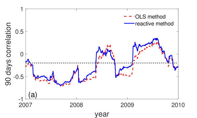
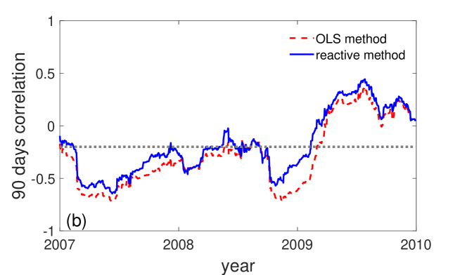
Figure 5: Ninety-day correlation of the low volatility factor with the stock index in the European market (a) and in the USA market (b). Solid and dashed lines present the proposed the reactive beta model and the OLS methodology, respectively. The dotted horizontal line shows the selection bias of $-19.10\%$, as shown in Appendix A. A time frame surrounding the financial crisis is chosen. Period: 2007-2010.

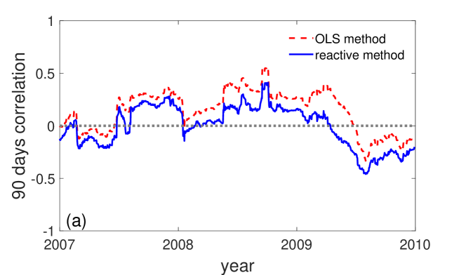
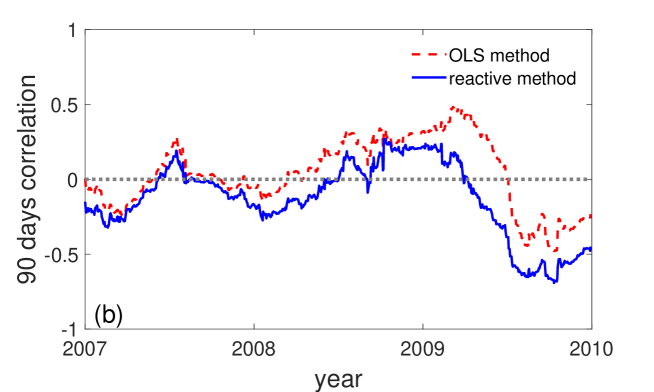
Figure 6: Ninety-day correlation of the short-term reversal factor with the stock index in the European market (a) and in the USA market (b). Solid and dashed lines present the proposed Reactive beta model and the OLS methodology, respectively. A time frame surrounding the financial crisis is chosen. Period: 2007-2010.

4 Robustness Checks

This section presents robustness check analysis by comparing the quality of several methods for beta measurements against the reactive beta model. We build the comparative analysis based on two important articles in order to explore two aspects of the beta estimation. Chan and Lakonishok (1992) enable to assess robustness statistics of some alternatives methods to classical ordinary least square (OLS) when assuming implicitly that betas are static and returns are homoscedastic. This section extends their work by including alternative dynamics beta estimators to be coherent with our reactive model and with the work by Engle (2016) that demonstrates that the betas are significantly time-varying using dynamic conditional betas. The presentation of the models and methods are located in the Appendix B.1.

4.1 Monte Carlo simulations

In financial research, one often resorts to simulated data to estimate the error of measurements. For instance, Chan and Lakonishok (1992) built their main results on numerical simulation while applying real data for simple comparison between betas estimated with OLS and quantile regression (QR).

The comparative analysis is based on a two-step procedure. The first step simulates returns using different models that capture some markets patterns and the second step estimates the beta from simulated returns by using our reactive method and alternative methods. We tested the same estimators as used by Chan and Lakonishok (1992) that includes the OLS, the minimum absolute deviation (ABSD), and the Trimean quantile regression (TRM). We also added two variations of the dynamical conditional correlation (DCC) which has become a mainstream model to measure conditional beta when beta is stochastic (Bollerslev et al., 1988; Bollerslev, 1990; Engle, 2002; Cappiello et al., 2006). We analyze the error of measurements that we defined as the difference between the measured beta and the true beta of simulated data.

4.1.1 The first step: simulation

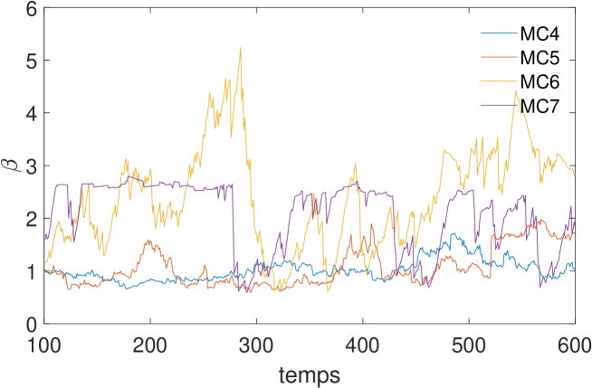
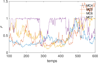
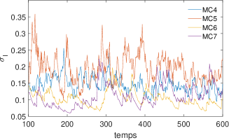
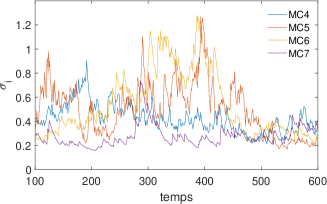
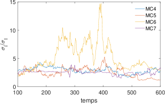
Figure 7: Simulated paths for the models MC4 – MC7. True conditional beta (top), true conditional correlation (middle left), true conditional stock index volatility (middle right), true conditional single stock volatility (bottom left), true conditional relative volatility (bottom right) are plotted. Paths limited to 500 days, that are independent from model to model, capture the same order of magnitude of variation in volatilities, beta and correlation.

The first step simulates 30,000 paths of $T$=1,000 consecutive returns for both the stock index and the single stock. It allows also to generate 1,000 conditional “true” expected beta per path (Fig. 7). To that end, following Chan and Lakonishok (1992), normally distributed residuals and Student-t distributed residuals are considered to take into consideration robustness of different methods to outliers.

In our setting, we implemented seven Monte Carlo simulations for the returns $r_{i}$ and $r_{I}$. We targeted in simulations the realistic case of an unconditional single stock annualized volatility of 40%, an unconditional stock index volatility of 15% and an unconditional beta of 1. That is important to target the realistic correlation between the index and the stock of 0.4. Indeed the relative precision of the beta measurement is inversely proportional to the square root of the number of returns when correlation is close to zero. First, we consider the naive version of the market model, based on Eq. (11), that we call “the basic market model” For the case of constant beta, as in paper by Chan and Lakonishok (1992), the simulated data are based on the hypothesis of a null intercept and beta is equal to $1$ to characterize the ideal case with a Gaussian (MC1) or a t-student distribution (MC2) for residuals. In the most simple reactive version of the market model that we call “the reactive market model”, normalized returns $\tilde{r}_{i}$ and $\tilde{r}_{I}$ are first generated randomly through Eq. (12) with a normalized beta set to 1. Then, based on the level $L_{s}$, $L_{is}$ that are respectively the slow moving averages of the stock index and the stock prices defined in Eq. (1), we generate $\delta I$ and $\delta S$ defined in Eq. (6), then $r_{i}$ and $r_{I}$, and finally update $L_{s}$ and $L_{is}$ . That model is sufficient to capture the leverage effect on beta with increasing beta as soon as single stock underperforms the stock index. Even if the normalized beta is set to unity (MC3 and MC4), the denormalized beta in Eq. (13) becomes time dependent (Fig. 7). As previously, MC3 and MC4 differ by the distribution of residuals, Gaussian (MC3) versus Student-t (MC4).

For the case of time-varying beta (MC 3 to 5), we used two versions of the reactive market model in Eq. (12): the reduced version with only the leverage effect components that is enough to generate stochastic beta in Eq. (13), and the full version with all components including the nonlinear beta elasticity. For the full version (MC5), we generated stochastic $\tilde{\sigma}_{i}$ and $\tilde{\sigma}_{I}$ that generate $\tilde{r}_{i}$ and $\tilde{r}_{I}$ from Eq. (12) using the normalized beta fixed to $\mathcal{F}(t)\mathcal{L}(t)$ (see definitions in Eqs. (31) and (21)). That allows to generate returns that capture the leverage effect pattern and the empirical non-linear beta elasticity (Fig. 3 and Fig. 4).

For the case of time-varying beta (MC 6 to 7), we used another way to generate random returns that capture a time-varying beta through the implementation of the dynamic conditional correlation (DCC) model (Engle, 2002), which generalizes the GARCH(1,1) process to two dimensions. This is a mainstream model which has two variations: symmetric and asymmetric, the latter capturing the leverage effect. Symmetric and asymmetric versions of DCC model are denoted as MC6 and MC7.

To summarize, seven Monte Carlo simulations:

• MC 1: The basic market model in Eq. (12) where residuals ($\epsilon_{i}$) are normally distributed and constant beta is set to 1.

• MC 2: The basic market model in Eq. (12) where residuals ($\epsilon_{i}$) follow a Student-t distribution (with three degrees of freedom) and constant beta is set to 1.

• MC 3: The reduced reactive market model in Eq. (12) where residuals ($\tilde{\epsilon}_{i}$) are normally distributed with constant volatilities ($\tilde{\sigma}_{i}$, $\tilde{\sigma}_{I}$) and constant renormalized beta ($\tilde{\beta}$) set to 1 but the denormalized beta is now depending on time (Fig 7). The conditional beta ($\beta$) is now a mean reversion process with a relaxation time $1/\lambda_{s}=50$ days. MC3 uses only the leverage effect component but not the nonlinear beta elasticity.

• MC 4: The reduced reactive market model in Eq. (12) where residuals ($\tilde{\epsilon}_{i}$) follow a Student-t distribution (with three degrees of freedom) with constant relative volatility and constant renormalized beta set to 1.

• MC 5: The full reactive market model in Eq. (12) where residuals ($\tilde{\epsilon}_{i}$) follow a Student-t distribution (with three degrees of freedom) whose standard deviation ($s_{i}$) is stochastic and where the normalized stock index return ($\tilde{r}_{I}$) is a Gaussian whose standard deviation ($s_{I}$) is also stochastic. We suppose that $\log(s_{I})$ and $\log(s_{i})-\log(S_{I})$ follow two independent Ornstein-Uhlenbeck processes (with the relaxation time of 100 days and the volatility of volatility of 0.04). In that way the stock index annualized volatility could jump up to 40%. Normalized beta, that was set to 1 in MC4, is now set to $\mathcal{F}(t)\mathcal{L}(t)$ to take into account the nonlinear beta elasticity (see definitions in Eqs. (31) and (21)). Both leverage effect and stochastic normalized volatilities make the beta defined in Eq. (36) )and volatilities time-depended (Fig. 7).

• MC 6: The symmetric DCC model in two dimensions, which generates volatilities of volatilities and correlation of similar amplitude as MC5 (Fig. 7).

• MC 7: The ADCC model in two dimensions, which generates volatilities of volatilities and correlation of similar amplitude as MC5 (Fig. 7).

In Fig. 7, we plot a Monte Carlo path generated for true beta for MC 3 to 7 (MC1 and MC2 are excluded as they generate true beta of 1). We also plot the conditional correlation and volatilities that are highly volatile and make the estimation of the conditional beta complicated.

4.1.2 The second step: measurements

The second step is devoted to the analysis of the error measurement of the beta estimations defined as the difference between the measured beta and the true beta of simulated data. In our setting, we test 5 alternative beta estimations that should replicate as close as possible the true beta. Notice that in all five configurations, we use an exponentially weighted scheme to give more weight to recent observations to be in line with the reactive market model ($1/\lambda_{\beta}=90$). As a consequence, in a path of $T$=1,000 generated returns, only the 90 last returns really matters (note that Chan and Lakonishok (1992) based their statistics on 35 returns with an equal weight scheme). The first alternative method is the Ordinary Least Square (OLS) of the returns which was also implemented in the empirical test based on real data. Note that the OLS would give the same measurement than our reactive method if parameters were set differently ($\lambda_{s}=1$, $\lambda_{f}=1$, $l=l^{\prime}=0$, $f=0$). The square errors in the OLS are weighted by $(1-\lambda_{\beta})^{T-t}$. The second method estimates the beta by using the Minimum Absolute Deviation (MAD) that is supposed to be less sensitive to outliers as absolute errors instead of square errors are minimized. The absolute errors are weighted by $(1-\lambda_{\beta})^{T-t}$. The third alternative is the beta computed from the Trimean quantile regression (TRM) that is reputed to be more robust to outliers according to Chan and Lakonishok (1992). The absolute errors are also weighted by $(1-\lambda_{\beta})^{T-t}$. The fourth and fifth methods are the conditional beta computed from the DCC model. The DCC method was calibrated using the same exponential $(1-\lambda_{\beta})^{T-t}$ weights introduced in the log-likelihood function to extract the optimal unconditional volatilities and correlations, while other parameters such as the relaxation time and volatilities of volatilities and volatilities of correlations were set to the values that were used for Monte Carlo simulation.

We summarize the reactive method and the five alternative methods that were implemented to estimate the beta:

• $\beta_{OLS}$: beta estimated by the Ordinary Least Square method;

• $\beta_{MAD}$: beta estimated by the Minimum Absolute Deviation method;

• $\beta_{TRM}$: beta estimated by the Trimean Quantile regression;

• $\beta_{DCC}$: $T^{\rm th}$ conditional beta estimated by using the DCC model;

• $\beta_{ADCC}$: $T^{\rm th}$ conditional beta estimated by using the ADCC model;

• $\beta_{R}$: beta estimated by the reactive method in Eq. (36).

4.1.3 The statistics

We analyze for every path the error of measurement defined as the difference between the measured beta based on different methods applied to $T$ returns and the true value of beta at time $T$.

To assess the quality of different methods, we use three statistics following Chan and Lakonishok (1992). The first statistics is the bias and gives the average error of measurement. Yielding the bias is more informative than simply yielding an estimated average estimation of beta as in our case the theoretical expected simulated conditional beta is not always 1 but fluctuates around 1 for time-varying models from MC3 to MC6. As we focused on capturing the leverage effect in the beta measurement we also define winner (loser) stocks that are the stocks that have outperformed (underperformed) the stock index during the last month. Due to the leverage effect, the OLS method is expected to underestimate beta for loser stocks and to overestimate beta for winner stocks. It would be interesting to see how robust is the improvement of the reactive beta. We therefore measure the average error among the loser and winner stocks. The loser and winner biases are related to the bias in hedging of the short term reversal strategy measured on real data and could confirm the robustness of the empirical measurements. We also define the low (high) beta stocks that are the stocks whose conditional true beta is lower (higher) than 1. We measure the average error among low and high beta stocks that are related to the bias in hedging of the low beta strategy measured from real data and could confirm the robustness of the beta measurement when adding the component describing the nonlinear beta elasticity.

The second statistics is the ABSolute Deviation (ABSD) of measurement. It reflects the average absolute errors such that the positive and negative sign errors cannot be mutually compensated. It is a measurement of the robustness. The third statistics, that is equivalent to ABSD, is the inverse of the variance of the errors of measurement ($\frac{V_{OLS}}{V_{m}}$) to characterize the relative robustness of the alternative beta estimation. The alternative beta method (with subscript $m$) that brings the highest improvement is the one with the highest ratio.

The three statistics that were implemented are summarized:

• Statistics 1: the bias, the winner bias and the loser bias, the low bias and the high bias;

• Statistics 2: the absolute deviation of measurement (ABSD);

• Statistics 3: the relative variance statistics $\frac{V_{OLS}}{V_{m}}$.

4.2 Empirical tests

We summarize statistics in Table 2. We see that all methods are unbiased on average in most Monte Carlo simulations. But this is misleading as biases from one group of stocks can be significant and offset others.

4.2.1 Winner and loser bias

The estimated $\beta_{DCC}$ and $\beta_{ADD}$ appear to be biased as soon as fat tails are included (MC2).

The reactive beta is the only one to be unbiased for winner and loser stocks when the leverage effect is introduced in Monte Carlo (MC 3, 4, 5). The biases for winner stocks and loser stocks are significant for all methods except for the reactive beta. The biases are amplified when a fat tail of residuals distribution is introduced (MC 4). Winner/loser biases can reach 14%. That is in line with the empirical test implemented on real data where we see that the reactive method reduces the bias of hedging of the short-term reversal strategy (Tab. 1).

When all components that deviate from the Gaussian market model are mixed in MC5 (fat tails, nonlinear beta elasticity, stochastic volatilities, leverage effect) we see a kind of cocktail effect as bias is generated for most methods on average and not only in some groups of stocks. The reactive method provides the best results and is the only method that has no bias. $\beta_{MAD}$ and $\beta_{TRM}$ that were supposed to be robust appear to perform very badly with high bias (average, loser or winner) as soon as stochastic volatility is added that is confirmed with MC6 and MC7.

We also see that the reactive model looks to be incompatible with the DCC or ADCC model. Indeed MC5 generates high bias for $\beta_{DCC}$ and $\beta_{ADD}$ in the winner and loser stocks even if the leverage effect and the dynamic beta are implemented in the ADCC. In the same way MC 6 generates bias for the reactive method that are even amplified when leverage effect is generated through MC7. We can wonder which model is the most realist. Both ADCC and the reactive model capture the volatility clustering and leverage effect patterns but their dynamics is in reality very different. In the reactive model, volatility increases as soon as price decreases, and decreases as soon as price increases whereas ADCC needs to see its volatility increase a negative return, higher than expected ($\gamma\left(\sigma_{i}^{2}[\xi_{i}^{-}(t)]^{2}-\tilde{\sigma}_{i}^{2}\right)>0$, see Eqs. (67, 69)). The reactive beta model has its three components that were fitted to three well identified effect (the specific leverage through the retarded effect, the systematic leverage through the panic effect and the non linear beta elasticity) whose main parameters appears to be stable and universal for all markets. Bouchaud et al. (2001) measured most of the parameters for 7 main stock indexes. Relaxation time is around 1 week for the panic effect ($\lambda_{s}=0.1484$), relaxation is 40 days for the retarded effect ($\lambda_{s}=0.0241$), the leverage parameter for the panic effect is $l=8$. The systematic leverage parameter $\ell-\ell^{\prime}=0.91$ was the only one to have been measured through the implied correlation only from the US market. The parameters of the beta elasticity were measured similar for both the European and the US market. The different thresholds are $0.5$ and $1.6$ in beta of the non linear beta elasticity separating low beta stocks from speculative stocks). Parameters $a$, $b$, $\gamma$, $a_{\rho}$, $b_{\rho}$, $\gamma_{\rho}$ of the DCC and ADCC were based on the work by Sheppard (2017) but $b$ and $b_{\rho}$ which are the “decay coefficients”, describe relaxation times of 10 days and 13 days that are different from those used in the reactive volatility model.

4.2.2 High and low beta bias

The reactive beta is the only one that reduces the bias for low and high beta stock when stochastic volatility is introduced and when the empirical nonlinear beta elasticity is implemented (MC 5). That is in line with the empirical test implemented on real data where we see that the reactive method reduces the bias of hedging of the low volatility strategy (Tab. 1).

4.2.3 ABSD and $V_{OLS}/V_{m}$

The $\beta_{OLS}$, that is the theoretical optimal estimation for Monte Carlo simulated returns with the Gaussian market model (MC1), gives similar statistics to that of the reactive beta for the MC3. In this case (MC3), the reactive method outperforms the other considered methods. The ABSD of 0.17 is entirely explained by irreducible statistical noise that is intrinsic to any regression based on approximately 90 points with a weak correlation.

When a fat tail is incorporated to the residual (MC4), the ABSD of the reactive beta is increased and becomes intermediate between the ABSD of $\beta_{OLS}$, $\beta_{MAD}$ and $\beta_{TRM}$. $\beta_{MAD}$ and $\beta_{TRM}$ are more robust in presence of fat tails. The reactive beta is expected to be as sensitive as the OLS would be due to the outliers. The reactive method could be still improved if a TRM regression was implemented instead of the classical OLS to measure the normalized beta between normalized returns. When stochastic volatility and correlation are introduced (MC5, MC6 and MC7), the reactive beta becomes as robust as $\beta_{MAD}$ and $\beta_{TRM}$ based on ABSD.

Method	Bias	Winner Bias	Loser Bias	Low Bias	High Bias	ABSD	Vols/Vm
MC1 Gaussian basic market model
$\beta_{OLS}$	-0.00	-0.00	-0.00			0.16	1.00
$\beta$ Reactive	0.00	-0.05*	0.05*			0.18	0.79
$\beta_{DCC}$	0.04*	0.05*	0.03*			0.23	0.51
$\beta_{ADCC}$	0.09*	0.01	0.17*			0.25	0.44
$\beta_{MAD}$	-0.00	0.00	-0.01			0.20	0.65
$\beta_{TRM}$	-0.00	0.00	-0.01			0.20	0.68
MC2 t-Student basic market model
$\beta_{OLS}$	-0.00	0.01	-0.01			0.28	1.00
$\beta$ Reactive	0.01	-0.06*	0.08*			0.31	0.82
$\beta_{DCC}$	0.13*	0.14*	0.12*			0.39	0.67
$\beta_{ADCC}$	0.25*	0.15*	0.35*			0.46	0.57
$\beta_{MAD}$	-0.00	-0.00	-0.00			0.22	2.18
$\beta_{TRM}$	-0.00	-0.00	-0.00			0.22	2.24
MC3 Gaussian reduced reactive market model
$\beta_{OLS}$	-0.00	0.07*	-0.07*	0.07*	-0.07*	0.19	1.00
$\beta$ Reactive	-0.00	0.02*	-0.02*	0.02*	-0.02*	0.17	1.27
$\beta_{DCC}$	0.04*	0.10*	-0.02	0.11*	-0.02	0.24	0.62
$\beta_{ADCC}$	0.09*	0.06*	0.12*	0.07*	0.11*	0.24	0.66
$\beta_{MAD}$	-0.01	0.06*	-0.08*	0.06*	-0.08*	0.22	0.73
$\beta_{TRM}$	-0.01	0.06*	-0.08*	0.06*	-0.08*	0.22	0.75
MC4 t-Student reduced reactive market model
$\beta_{OLS}$	0.01	0.13*	-0.11*	0.12*	-0.10*	0.35	1.00
$\beta$ Reactive	-0.01	0.02	-0.04*	0.03	-0.05*	0.31	1.30
$\beta_{DCC}$	0.12*	0.22*	0.02	0.27*	-0.01	0.47	0.84
$\beta_{ADCC}$	0.26*	0.24*	0.28*	0.30*	0.21*	0.52	0.83
$\beta_{MAD}$	-0.03*	0.09*	-0.14*	0.10*	-0.14*	0.27	2.68
$\beta_{TRM}$	-0.03*	0.09*	-0.14*	0.10*	-0.14*	0.27	2.76
MC5 t-Student full reactive market model
$\beta_{OLS}$	-0.01	0.13*	-0.14*	0.14*	-0.22*	0.50	1.00
$\beta$ Reactive	-0.04*	-0.00	-0.07*	0.05*	-0.17*	0.41	1.42
$\beta_{DCC}$	-0.01	0.10*	-0.12*	0.20*	-0.32*	0.52	1.31
$\beta_{ADCC}$	0.10*	0.10*	0.11*	0.29*	-0.17*	0.54	1.32
$\beta_{MAD}$	-0.09*	0.04*	-0.22*	0.09*	-0.37*	0.38	2.43
$\beta_{TRM}$	-0.09*	0.04*	-0.22*	0.09*	-0.36*	0.37	2.46
MC6 Gaussian symmetric DCC model
$\beta_{OLS}$	-0.11*	-0.10*	-0.11*	0.06*	-0.27*	0.32	1.00
$\beta$ Reactive	-0.07*	-0.11*	-0.02	0.09*	-0.23*	0.33	0.93
$\beta_{DCC}$	-0.01	-0.00	-0.02*	-0.01	-0.01	0.16	4.09
$\beta_{ADCC}$	0.02*	-0.08*	0.12*	0.05*	-0.01	0.22	2.06
$\beta_{MAD}$	-0.14*	-0.13*	-0.15*	0.04*	-0.32*	0.34	0.89
$\beta_{TRM}$	-0.14*	-0.13*	-0.15*	0.04*	-0.32*	0.34	0.90
MC7 Gaussian asymmetric DCC model
$\beta_{OLS}$	-0.09*	0.03	-0.24*	0.09*	-0.25*	0.30	1.00
$\beta$ Reactive	-0.07*	0.02	-0.17*	0.10*	-0.21*	0.27	1.21
$\beta_{DCC}$	-0.04*	0.04*	-0.15*	-0.00	-0.08*	0.21	2.08
$\beta_{ADCC}$	-0.01	-0.01	-0.01	-0.00	-0.01	0.15	3.74
$\beta_{MAD}$	-0.13*	-0.02	-0.28*	0.06*	-0.29*	0.32	0.92
$\beta_{TRM}$	-0.13*	-0.01	-0.28*	0.06*	-0.29*	0.32	0.92

Table 2: Monte-Carlo robustness test. Statistics are provided for seven Monte Carlo simulations and six different methods to estimate the beta. We estimated the statistics such as the bias that is the average error of beta measurement; winner/loser biases are the biases among winner/loser stocks. Low/High biases are the biases among low/high beta stocks. * indicates a bias superior to 3 standard deviation. ABSD is the average of the error in absolute value. Vols/Vm is the variance of the error in the OLS case divided by the variance of the error.

5 Open problems in other fields

The estimated beta is used in a wide range of financial applications, which includes security valuation, asset pricing, portfolio management and risk management. This extends also to corporate finance in many applications such like financing decisions to quantify risk associated with debt, equity and asset and for firm valuation when discounting cash-flows using the weighted average cost of capital. The most likely reason is that the beta describes systematic risk that could not be diversified and that should should be remunerated. However as explained, the OLS estimator of beta is subject to measurement errors, which include the presence of outliers, time dependence, the leverage effect, and the departure from normality.

5.1 Asset Pricing

Bali et al. (2017) apply the DCC model by Engle (2016) to assess the cross-sectional variation in expected stock returns. They estimate the conditional beta for the S&P 500 using daily data for each year from 1963 to 2009. They test if the betas have predictive power for the cross-section of individual stocks returns over the next on to five days. They show that there is no link between the unconditional beta and the cross-section of expected returns. Most remarkably, they also show that the time-varying conditional beta is priced in the cross-section of daily returns. At the portfolio level, they indicate that a long-short trading strategy buying the highest conditional beta stocks and selling the lowest conditional beta stocks yields average returns of 8% per year. So conditional CAPM is empirically valid whereas unconditional CAPM is empirically not valid. Moreover they showed that conditional beta when comparing to unconditional beta would not have significant pricing effect on major anomalies (size, book, momentum,…). So one can see that DCC greatly improves the empirical validation of the CAPM but does not change pricing of anomalies. We expect that the reactive method can bring further improvements. According to our robustness tests in Sec. 4, the leverage effect and the nonlinear beta elasticity could also generate bias in the DCC estimation. As our reactive method was designed to correct for these biases, its use can help to reveal pricing effects of the dynamic beta on major anomalies. This point is an interesting perspective for future research.

5.2 Corporate Finance

To determine a fair discount rate for valuing cash-flows, the firm’s manager must select the appropriate beta of the project given that the discount rate remains constant over time while the project may exhibit significant variation over time and leverage effect due to the debt-to-equity ratio. As such, Ang and Liu (2004) discuss how to discount cash-flows with time-varying expected returns in traditional set-up. For instance, the traditional dividend discount model assumes that the expected return along with the expected rate of cash-flow growth are set constant while they are time-varying and correlated. In practice, in the first step, the manager computes the expected future cash-flows from financial forecasts and then in a second step, the manager uses a constant discount rate, usually relying on the CAPM to discounting factor. In contrast, Ang and Liu (2004) derive a valuation formula that incorporates correlation between stochastic cash-flows, betas and risk premiums. They show that the greater the magnitude of the difference between the true discount rates and the constant discount rate, the greater the project’s misvaluation. They even show that when computing perpetuity values from the discounting model, the potential mispricing can even get worse. They conclude that accounting for time-varying expected returns can lead to different prices from using a constant discount rate from the traditional unconditional CAPM. The impact of the leverage effect and of the non-linear elasticity of beta on potential mispricing should be investigated.

6 Conclusion

We propose a reactive beta model with three components that account for the specific leverage effect (when a stock underperforms, its beta increases), the systematic leverage effect (when a stock index declines, correlations increase), and beta elasticity (when relative volatility increases, the beta increases). The three components were fitted and incorporated through elaborate statistical measurements. An empirical test is run from 2000 to 2015 with exhaustive data sets including both American and European securities. We compute the bias in hedging the most popular market neutral strategies (low volatility, momentum and capitalization) using the standard approach of the beta measurement and the reactive beta model. Our main findings emphasize the ability of the reactive beta model to significantly reduce the biases of these strategies, particularly during stress periods. Robustness check confirms that the reactive beta is not biased when the leverage effect and beta elasticity are introduced and appear to be robust when volatility of volatility and volatility of correlation are introduced.

Appendix A Selection bias

Here, we provide some evidence that the bias in beta of the low volatility factor comes from the selection bias: selection of the bottom beta stocks yields the stocks whose beta is underestimated.

The measured beta $\beta_{im}$ of stock $i$ is obtained by a standard linear regression of the $i$-th stock returns, $r_{i}$, to the stock index returns, $r_{I}$,

$$r_{i}=\beta_{im}r_{I}+\epsilon_{i},$$ (37)

where $\epsilon_{i}$ is the residual return. We suppose that the measured beta of the stock $i$, $\beta_{im}$, is affected by noise,

$$\beta_{im}=\beta_{iT}+\eta_{i},$$ (38)

where $\beta_{iT}$ is the true beta (which is unknown), and $\eta_{i}$ is the error of the measurement inherent to the linear regression. The standard deviation of $\eta_{i}$, $\sigma_{\eta_{i}}$, depends on the average correlation between the single stock $i$ and the stock index and on the number $n$ of independent points used for the regression (which we set at $n=\frac{1}{\lambda_{\beta}}=90$):

$$\sigma_{\eta_{i}}=\frac{\sigma_{\epsilon i}}{\sigma_{I}}\,\frac{1}{\sqrt{n}},$$ (39)

where $\sigma_{\epsilon i}$ is the standard deviation of the residual returns $\epsilon_{i}$. Averaging the above relation over all stocks, we obtain

$$\sigma_{\eta}=\frac{\langle\sigma_{\epsilon i}\rangle}{\sigma_{I}}\sqrt{\lambda_{\beta}},$$ (40)

where $\langle\sigma_{\epsilon i}\rangle$ denotes the average. According to Eq. (37), the standard deviation of the stock returns, $\sigma_{i}$, is

$$\sigma_{i}=\sqrt{\beta_{im}^{2}\sigma_{I}^{2}+\sigma_{\epsilon i}^{2}}\approx\sigma_{\epsilon i},$$ (41)

because $(\beta_{im}\sigma_{I}/\sigma_{i})^{2}\ll 1$ (stocks are much more volatile than the index). We thus obtain

$$\sigma_{\eta}\approx\frac{\langle\sigma_{i}\rangle}{\sigma_{I}}\sqrt{\lambda_{\beta}}.$$ (42)

The low volatility factor is 50% long of the 30% top $\beta_{im}$ stocks and 50% short of the 30% bottom $\beta_{im}$ stocks (here, we consider only one sector for simplicity). We adjust the most volatile leg to target a beta neutral factor if we suppose that $\eta_{i}$ are null. In reality, when taking into account the difference between the measured and the true beta, we obtain the beta of the low volatility factor as:

$$\beta_{\textrm{low factor}}=-50\%\langle\beta_{iT}|i\in\textrm{Bottom}\rangle+50\%\frac{\langle\beta_{im}|i\in\textrm{Bottom}\rangle}{\langle\beta_{im}|i\in\textrm{Top}\rangle}\langle\beta_{iT}|i\in\textrm{Top}\rangle.$$ (43)

This is essentially the beta neutral condition that we impose when constructing the factor (see Appendix B). Here, $\langle\beta_{im}|i\in\textrm{Bottom}\rangle$ is the average of the measured beta over the stocks $i$ in the 30% bottom in the measured beta values $\beta_{im}$ (similar for other averages).

Defining $\Delta\beta_{B}$ and $\Delta\beta_{T}$ as

$$\langle\beta_{iT}|i\in\textrm{Bottom}\rangle=\langle\beta_{im}|i\in\textrm{Bottom}\rangle+\Delta\beta_{B},$$ (44)

$$\langle\beta_{iT}|i\in\textrm{Top}\rangle=\langle\beta_{im}|i\in\textrm{Top}\rangle+\Delta\beta_{T},$$ (45)

we rewrite Eq. (43) as

$$\beta_{\textrm{low factor}} = -50\%\left(\langle\beta_{im}|i\in\textrm{Bottom}\rangle+\Delta\beta_{B}\right)+50\%\frac{\langle\beta_{im}|i\in\textrm{Bottom}\rangle}{\langle\beta_{im}|i\in\textrm{Top}\rangle}\left(\langle\beta_{im}|i\in\textrm{Top}\rangle+\Delta\beta_{T}\right)$$ (46)

$$= -50\%\Delta\beta_{B}+50\%\frac{\langle\beta_{im}|i\in\textrm{Bottom}\rangle}{\langle\beta_{im}|i\in\textrm{Top}\rangle}\Delta\beta_{T}.$$

Given that $\langle\beta_{im}|i\in\textrm{Bottom}\rangle\ll\langle\beta_{im}|i\in\textrm{Top}\rangle$ (as the $\beta_{im}$ in the top quantile are higher than the $\beta_{im}$ in the bottom quantile), we obtain the following approximation

$$\beta_{\textrm{low factor}}\approx-50\%\Delta\beta_{B}.$$ (47)

If one knew the true $\beta_{iT}$ values and used them for constructing the low volatility factor, the excess $\Delta\beta_{B}$ would be zero. However, the true values are unknown, and one uses the measured beta $\beta_{im}$ that creates a selection bias and the nonzero $\Delta\beta_{B}$, as shown below.

To estimate $\Delta\beta_{B}$, we consider the true beta $\beta_{iT}$ and the measurement error $\eta_{i}$ as independent random variables and replace the average over stocks by the following conditional expectation

$$\Delta\beta_{B}=\langle\beta_{iT}-\beta_{im}|i\in\textrm{Bottom}\rangle\approx{\mathbb{E}}\{\beta_{iT}-\beta_{im}|i\in\textrm{Bottom}\}=B.$$ (48)

We have, then,

$$-B = {\mathbb{E}}\{\eta_{i}|i\in\textrm{Bottom}\}=\int\limits_{-\infty}^{\infty}\eta\,{\mathbb{P}}\{\eta_{i}\in(\eta,\eta+d\eta)|i\in\textrm{Bottom}\}$$ (49)

$$= \int\limits_{-\infty}^{\infty}\eta\,\frac{{\mathbb{P}}\{\eta_{i}\in(\eta,\eta+d\eta),\leavevmode\nobreak\ i\in\textrm{Bottom}\}}{{\mathbb{P}}\{i\in\textrm{Bottom}\}},$$

where we wrote explicitly the conditional probability. The denominator is precisely the threshold determining the bottom quantile, ${\mathbb{P}}\{i\in\textrm{Bottom}\}=p$, which we set to $30\%$. We thus obtain

$$-B=\frac{1}{p}\int\limits_{-\infty}^{\infty}\eta\,{\mathbb{P}}\{\eta_{i}\in(\eta,\eta+d\eta),\leavevmode\nobreak\ \beta_{im}-\beta_{0}<Q\},$$ (50)

where the event $i\in\textrm{Bottom}$ is equivalently written as $\beta_{im}<\beta_{0}+Q$, where $Q$ is the value of the measured beta that corresponds to the quantile $p$, and $\beta_{0}$ is the mean of $\beta_{im}$. Using Eq. (38) and the assumption that $\beta_{iT}$ and $\eta_{i}$ are independent, one obtains

$$-B = \frac{1}{p}\int\limits_{-\infty}^{\infty}\eta\,{\mathbb{P}}\{\eta_{i}\in(\eta,\eta+d\eta),\leavevmode\nobreak\ \beta_{iT}-\beta_{0}<Q-\eta\}$$ (51)

$$= \frac{1}{p}\int\limits_{-\infty}^{\infty}\eta\,{\mathbb{P}}\{\eta_{i}\in(\eta,\eta+d\eta)\}\,{\mathbb{P}}\{\beta_{iT}-\beta_{0}<Q-\eta\}.$$

To obtain some quantitative estimates, we make a strong assumption that both $\beta_{iT}$ and $\eta_{i}$ are Gaussian variables, with means $\beta_{0}$ and $0$ and standard deviations $\sigma_{\beta}$ and $\sigma_{\eta}$, respectively. We then obtain

$$-B=\frac{1}{p}\int\limits_{-\infty}^{\infty}d\eta\,\eta\,\frac{\exp(-\eta^{2}/(2\sigma_{\eta}^{2}))}{\sqrt{2\pi}\,\sigma_{\eta}}\Phi\bigl{(}(Q-\eta)/\sigma_{\beta}\bigr{)},$$ (52)

where

$$\Phi(x)=\int\limits_{-\infty}^{x}dy\,\frac{e^{-y^{2}/2}}{\sqrt{2\pi}}$$ (53)

is the cumulative Gaussian distribution. Changing the integration variable, one obtains

$$-B=\frac{\sqrt{2}\sigma_{\eta}}{p\sqrt{\pi}}\int\limits_{-\infty}^{\infty}dx\,x\,\exp(-x^{2})\Phi\bigl{(}(Q-x\sqrt{2}\sigma_{\eta})/\sigma_{\beta}\bigr{)}.$$ (54)

Integrating by parts and omitting technical computations, we obtain

$$B=\frac{\sqrt{2}\sigma_{\eta}}{p\sqrt{\pi}}\,\frac{\sigma_{\eta}}{2\sigma_{\beta}\sqrt{1+b^{2}}}\exp\biggl{(}-\frac{a^{2}}{1+b^{2}}\biggr{)},$$ (55)

where $a=Q/(\sqrt{2}\sigma_{\beta})$ and $b=\sigma_{\eta}/\sigma_{\beta}$. Setting

$$Q=\sigma_{\beta}\sqrt{2}\,q,\qquad q=\textrm{erf}^{-1}(2p-1),$$ (56)

we obtain

$$B=\frac{\sigma_{\eta}}{p\sqrt{2\pi}}\,\frac{1}{\sqrt{1+(\sigma_{\beta}/\sigma_{\eta})^{2}}}\exp\biggl{(}-\frac{q^{2}}{1+(\sigma_{\eta}/\sigma_{\beta})^{2}}\biggr{)},$$ (57)

from which

$$\beta_{\textrm{low factor}}\approx-50\%\frac{\sigma_{\eta}}{p\sqrt{2\pi}}\,\frac{1}{\sqrt{1+(\sigma_{\beta}/\sigma_{\eta})^{2}}}\exp\biggl{(}-\frac{q^{2}}{1+(\sigma_{\eta}/\sigma_{\beta})^{2}}\biggr{)}.$$ (58)

From the data for the USA, we estimate the standard deviation of the measured beta ($\sigma_{\beta}=0.43$), the volatility of the stock index ($\sigma_{I}=19.77\%$), the volatility of the low volatility factor ($3.46\%$), and $\langle\sigma_{i}\rangle/\sigma_{I}=1.53$. Setting $\lambda_{\beta}=1/90$, we obtain from Eq. (42) $\sigma_{\eta}=1.53\,\sqrt{1/90}=0.1613$. For $p=0.3$ (bottom $30\%$), we obtain $q=-0.3708$ and, thus, $\beta_{\textrm{low factor}}\approx 0.0334$ from Eq. (58). Finally, we conclude that $\rho_{\textrm{low factor}}=3.34\%\frac{19.77\%}{3.46\%}=19.1\%$.

Appendix B Construction of the beta-neutral factors

We implement the four most popular strategies as four beta-neutral factors that are constructed as follows. First, we split all stocks into six supersectors of similar sizes to minimize sectorial correlations. For each trading day, the stocks of the chosen supersector are sorted according to the indicator (e.g., the capitalization) available the day before (we use the publication date and not the valuation date). The related indicator-based factor is formed by buying the first $pN$ stocks in the sorted list and shorting the last $pN$ stocks, where $N$ is the number of stocks in the considered supersector, and $p$ is a chosen quantile level. As described in Sec. 3.2, we use $p=0.15$ for short-term reversal and long-term momentum factors and $p=0.30$ for the capitalization and low volatility factors. The other stocks (with intermediate indicator values) are not included (weighted by $0$). To reduce the specific risk, the weights of the selected stocks are set inversely proportional to the stock’s volatility $\sigma_{i}$, whereas the weights of the remaining stocks are $0$. Moreover, the inverse stock volatility is limited to reduce the impact of extreme specific risk. Each trading day, we recompute the weight $w_{i}$ as follows

$$w_{i}=\left\{\begin{array}[]{c l}+\mu_{+}\min\{1,\sigma_{\rm mean}/\sigma_{i}\},&\qquad\textrm{if $i$ belongs to the first $pN$ stocks in the sorted list},\\ -\mu_{-}\min\{1,\sigma_{\rm mean}/\sigma_{i}\},&\qquad\textrm{if $i$ belongs to the last $pN$ stocks in the sorted list},\\ 0,&\qquad\textrm{otherwise,}\\ \end{array}\right.$$ (59)

where $\sigma_{\rm mean}=\frac{1}{N}(\sigma_{1}+\ldots+\sigma_{N})$ is the mean estimated volatility over the cluster of sectors. In this manner, the weights of low-volatility stocks are reduced to avoid strongly unbalanced portfolios concentrated in such stocks. The two common multipliers, $\mu_{\pm}$, are used to ensure the beta market neutral condition:

$$\sum\limits_{i=1}^{N}\beta_{i}w_{i}=0,$$ (60)

where $\beta_{i}$ is the sensitivity of stock $i$ to the market obtained either by an OLS or by our reactive method. In every case, the method to estimate beta uses the rolling daily returns and only past information to avoid the look-ahead bias. If the aggregated sensitivity of the long part of the portfolio to the market is higher than that of the short part of the portfolio, its weight is reduced by the common multiplier $\mu_{+}<\frac{1}{2pN}$, which is obtained from Eq. (60) by setting $\mu_{-}=\frac{1}{2pN}$ (which implies that the sum of absolute weights $|w_{i}|$ does not exceed $1$). In the opposite situation (when the short part of the portfolio has a higher aggregated beta), one sets $\mu_{+}=\frac{1}{2pN}$ and determines the reducing multiplier $\mu_{-}<\frac{1}{2pN}$ from Eq. (60). The resulting factor is obtained by aggregating the weights constructed for each supersector. We emphasize that the factors are constructed on a daily basis, i.e., the weights are re-evaluated daily based on updated indicators. However, most indicators do not change frequently, so the transaction costs related to changing the factors are not significant.

B.1 Appendix C: Description of alternative methods

B.1.1 Unconditional beta

The theory.

Chan and Lakonishok (1992) produce an empirical analysis that describes various robust methods for estimating constant beta as they provide an alternative to Ordinary Least Squares (OLS). Their method is built the work Koenker (1978) that provides robust alternatives to the sample mean using more complex linear combination of order statistics in order to face the case of non-Gaussian errors, which are the source of outliers. Instead of minimizing the sum of squared residuals, they consider an estimator that is based on minimizing the criterion including a penalty function $\varrho$ on the residuals $\epsilon$:

$$\sum_{t=1}^{T}\varrho_{\theta}(\epsilon_{t})$$ (61)

for $\varrho_{\theta}(\epsilon_{t})=\theta\left|\epsilon_{t}\right|$ if $\epsilon_{t}\geq 0,$ or $(1-\theta)\left|\epsilon_{t}\right|$ if $\epsilon_{t}<0$, where $0<\theta<1$.

Chan and Lakonishok (1992) minimize the sum of absolute deviations of the residuals $\epsilon_{it}$ from the market model, instead of the sum of squared deviations. The resulting minimum absolute deviations (MAD) estimator of the regression parameters corresponds to the special case of $\theta=1/2$ where half of the observations lie above the line, while half lie below. More generally, large or small values of the weight $\theta$ attach a penalty to observations with large positive or negative residuals. Varying $\theta$ between 0 and 1 yields a set of regression quantile estimates $\hat{\beta(\theta)}$ that is analogous to the quantiles of any sample of data. However, they recognize that MAD does not prove itself to be a clearly superior method and suggest that it may be improved via linear combinations of sample quantiles such like trimmed means.

For that reason, Chan and Lakonishok (1992) test different combinations of regressions quantiles serving as the basis for the robust estimators. They discuss the general case of trimmed regression quantile (TRQ) given as a weighted average of the regression quantile statistics:

$$\hat{\beta}_{\alpha}=(1-2\alpha)^{-1}\int_{\alpha}^{1-\alpha}\hat{\beta}(\theta)d\theta$$ (62)

where $0<\alpha<1/2$ and $0<\theta<1$.

More specifically, Chan and Lakonishok (1992) suggest a more straightforward and equivalent method that considers estimators that are finite linear combinations of regression quantiles (QR) and computationally simpler:

$$\beta_{\omega}=\sum_{i=1}^{N}\omega_{i}\hat{\beta}(\theta_{i})$$ (63)

where weights $0<\omega_{i}<1$, $i=1,...,N$ and $\sum_{i=1}^{N}\omega_{i}=1$. The specific case of weighted average is given by the Tukey’s trimean (TRM) estimator:

$$\hat{\beta}_{TRM}=0.25\hat{\beta}(1/4)+0.5\hat{\beta}(1/2)+0.25\hat{\beta}(3/4)$$ (64)

The application.

Their analysis is based mainly on simulated returns data although they add some tests with actual returns data. The main advantages of a simulation are that the true values of the underlying parameters are known, and that the extent of departures from normality can be controlled. They begin with a baseline simulation with 25,000 replications using data generated from a normal distribution and they also consider the case where the residual term is drawn from a Student-distribution with three degrees of freedom in order to explain the observed leptokurtosis in daily returns data. We follow the same methodology to assess the quality of the OLS, the MAD and the TRM beta estimators using Gaussian and t-Student residuals in the seven types of Monte Carlo simulations (MC1,…,MC7).

To replicate the exponential weight scheme of the reactive model ($\lambda_{\beta}=1/90$), Eq. (61) is replaced by

$$\sum_{t=1}^{T}\left(1-\lambda_{\beta}\right)^{T-t}\varrho_{\theta}(\epsilon_{t})$$ (65)

B.1.2 Conditional Beta

The theory.

The first application of time-varying beta was proposed in Bollerslev et al. (1988) since the beta was computed as the ratio of the conditional covariance to the conditional variance. Engle (2002) generalizes Bollerslev (1990) constant correlation model by making the conditional correlation matrix time-dependent with the Dynamic Conditional Correlation (DCC) model that constrains the time-varying conditional correlation matrix to be positive definite and the number of parameters to grow linearly by a two step procedure. The first step requires the GARCH variances to be estimated univariately. Their parameter estimates remains constant for the next step. The second stage is estimated conditioning on the parameters estimated in the first stage.

Hereafter, we extend the modeling of the DCC beta for inclusion of an asymmetric term in the conditional variance equation. In the case of asymmetry in the conditional variance, we select the GJR-GARCH(1,1) specification by Glosten et al. (1993), which assumes a specific parametric form with leverage effect in the conditional variance (DCC-GJR beta). The basic idea is that negative shocks at period $(t-1)$ have a stronger impact in the conditional variance at period $t$ than positive shocks. Notice that even though the conditional distribution is Gaussian, the corresponding unconditional distribution can still present excess kurtosis.

We select the ADCC model by Cappiello et al. (2006) to incorporate asymmetry in correlation. The case mixing asymetry in both located in the variance equation (GJR-GARCH) and in the correlation equation (ADCC) is examined (ADCC-GJR GARCH). In our paper the symmetric GARCH DCC will be called simply DCC and the asymmetric ADCC-GJR will be called simply ADCC

Let us consider $r_{i}$ and $r_{I}$ as the returns of a single stock and the stock index, respectively. We assume that their respective conditional variances follow a (GJR-)GARCH(1,1) specification. The stock return $r_{i}$ is defined by its conditional volatility, $\sigma_{i}$, and a zero-mean white noise $\xi_{i}(t)$:

$$r_{i}(t)=\sigma_{i}(t-1)\xi_{i}(t)$$ (66)

The conditional variation specification of the stock return is the following:

$$\sigma_{i}^{2}(t)=(1-a-b-\gamma/2)\tilde{\sigma}_{i}^{2}+a\sigma_{i}^{2}(t-1)[\xi_{i}(t)]^{2}+b\sigma_{i}^{2}(t-1)+\gamma\sigma_{i}^{2}[\xi_{i}^{-}(t)]^{2}$$ (67)

where $\tilde{\sigma}_{i}$ is the unconditional volatility, and $a$, $b$, and $\gamma$ are parameters reflecting respectively, the ARCH, GARCH and asymmetry effects. When $\gamma=0$, the specification collapses to a GARCH model, otherwise, it stands for the GJR-GARCH model, where the asymmetric term is defined such as $\xi_{i}^{-}(t)=\xi_{i}(t)$ if $\xi_{i}(t)>0$, otherwise $\xi_{i}^{-}(t)=0$.

The stock index return $r_{I}$ is defined by its conditional volatility, $\sigma_{I}$, and a zero-mean white noise $\xi_{I}(t)$ that is correlated to $\xi_{i}(t)$:

$$r_{I}(t)=\sigma_{I}(t-1)\xi_{I}(t)$$ (68)

The conditional variance specification of the stock index return is the following:

$$\sigma_{I}^{2}(t)=(1-a-b-\gamma/2)\tilde{\sigma}_{I}^{2}+a\sigma_{I}^{2}(t-1)[\xi_{I}(t)]^{2}+b\sigma_{I}^{2}(t-1)+\gamma\sigma_{I}^{2}[\xi_{I}^{-}(t)]^{2}$$ (69)

We define the normalized conditional variance diagonal terms such as:

$$q_{ii}(t)=(1-a_{\rho}-b_{\rho}-\gamma_{\rho}/2)+a_{\rho}\xi_{i}(t-1)\xi_{i}(t-1)+b_{\rho}q_{ii}(t-1)+\gamma_{\rho}\xi_{i}^{-}(t-1)\xi_{i}^{-}(t-1)$$ (70)

$$q_{II}(t)=(1-a_{\rho}-b_{\rho}-\gamma_{\rho}/2)+a_{\rho}\xi_{I}(t-1)\xi_{I}(t-1)+b_{\rho}q_{II}(t-1)+\gamma_{\rho}\xi_{I}^{-}(t-1)\xi_{I}^{-}(t-1)$$ (71)

The normalized conditional covariance term $q_{iI}(t)$ is given by:

$$q_{iI}(t)=(1-a_{\rho}-b_{\rho}-\gamma_{\rho}/4)\tilde{\rho}+a_{\rho}\xi_{i}(t-1)\xi_{I}(t-1)+b_{\rho}q_{iI}(t-1)+\gamma_{\rho}\xi_{i}^{-}(t-1)\xi_{I}^{-}(t-1)$$ (72)

When $\gamma_{\rho}=0$, the specification collapses to a DCC model, otherwise it stands for the ADCC model, where the asymmetric term is defined such as $\xi_{i}^{-}(t)=\xi_{i}(t)$ if $\xi_{i}(t)>0$, otherwise $\xi_{i}^{-}(t)=0$.

The conditional correlation between $\xi_{I}(t+1)$ and $\xi_{i}(t+1)$ is then updated by:

$$\rho_{iI}(t)=q_{iI}(t)/\sqrt{q_{II}(t)q_{ii}(t)}$$ (73)

The beta DCC and beta ADCC estimation are defined in the same way:

$$\beta_{DCC}(t)=\rho_{iI}(t)\sigma_{i}(t)/\sigma_{I}(t)$$ (74)

The log-likelihood function is optimized to calibrate the parameters $\tilde{\rho}$, $\tilde{\sigma}_{I}$ and $\tilde{\sigma}_{i}$ for estimation:

$$L_{DCC}=\frac{1}{2}\sum_{t}^{T}\left(L_{V}(t)+L_{C}(t)\right)$$ (75)

$$L_{V}(t)=-2\log(2\pi)-\xi_{I}(t)^{2}-\xi_{i}(t)^{2}-2\log(\sigma_{I}(t))-2\log(\sigma_{i}(t))$$ (76)

$$L_{C}(t)=-\log(det(R(t)))-U^{\prime}(t)R(t)^{-1}U(t)-U^{\prime}(t)U(t)$$ (77)

with $det$ as the determinant of a matrix, and

$$R(t)=\begin{bmatrix}1&\rho_{iI}(t)\\ \rho_{iI}(t)&1\end{bmatrix},\qquad U(t)=\begin{bmatrix}\xi_{i}(t)\\ \xi_{I}(t)\end{bmatrix}$$ (78)

The application.

For Monte Carlo simulation purposes:

• $\xi_{i}(t)$ is either generated randomly in MC6 and MC7 according to a standard Gaussian or measured through returns $r_{i}(t)$ and $\sigma_{i}(t-1)$ for beta DCC estimation.

• $\gamma=0$ for MC6 and beta DCC estimation but $\gamma>0$ for MC7 and beta ADCC that captures the asymmetry term of the GJR-GARCH.

• $\xi_{I}(t)$ is either generated randomly in MC6 and MC7 according to a standard Gaussian random variable that is correlated to the random variable $\xi_{i}(t)$ (correlation between $\xi_{i}(t)$ and $\xi_{I}(t)$ is $\rho_{iI}(t-1)$) or measured through returns $r_{I}(t)$ and $\sigma_{I}(t-1)$ for beta DCC estimation.

• $\gamma_{\rho}=0$ for MC6 and beta DCC but $\gamma_{\rho}>0$ for MC7 and beta ADCC that captures the asymmetry term of the ADCC.

The fixed parameters that are supposed to be known when testing the beta DCC are set to US market estimates by from Sheppard (2017):

• fixed parameters for univariate symmetric GARCH(1,1) process (MC6, i.e. DCC):

  $b=0.89$, $b$ is the decay coefficient and $1/(1-b)$ is related to the number of days the process needs to mean revert;

  $a=0.099$ would describe the level of the volatility of the volatility.

• fixed parameters for univariate asymmetric GJR-GARCH(1,1,1) process (MC7, i.e., ADCC):

  $b=0.901$, $b$ is the decay coefficient and $1/(1-b)$ is related to the number of days the process needs to mean revert;

  $a=0.0$, $a+\gamma/2$ describe the level of the volatility of the volatility;

  $\gamma=0.171$, $\gamma$ would describe the asymmetry.

The fixed parameters that are supposed to be known when testing the beta DCC and betas ADCC are set to US market estimates from Cappiello et al. (2006):

• fixed parameters for the symmetric cross term process (MC6, i.e., DCC):

  $b_{\rho}=0.9261$, $b_{\rho}$ is the decay coefficient and is linked to the relaxation time;

  $a_{\rho}=0.0079$ would describe the level of the volatility.

• fixed parameters for the asymmetric cross term process (MC7, i.e., ADCC):

  $b_{\rho}=0.9512$, $b_{\rho}$ is the decay coefficient and is linked to the relaxation time;

  $a_{\rho}=0.0020$, $a_{\rho}+\gamma_{\rho}/4$ would describe the level of the volatility of the correlation;

  $\gamma_{\rho}=0.0040$, $\gamma_{\rho}$ would describe the asymmetry.

The fixed parameters that are not known when testing the beta DCC and estimated through optimization of log-likelihood are set by MC simulation to:

• $\tilde{\rho}=0.15/0.4$, unconditional correlation;

• $\tilde{\sigma}_{I}=0.15/\sqrt{255}$, $\tilde{\sigma}_{i}=0.4/\sqrt{255}$ unconditional stock index volatility;

• $\tilde{\sigma}_{i}=0.4/\sqrt{255}$ unconditional single stock volatility.

To replicate the exponential weight scheme in the reactive model ($\lambda_{\beta}=1/90$), Eq. (75) is replaced by

$$L_{DCC}=\frac{1}{2}\sum_{t}^{T}\left(1-\lambda_{\beta}\right)^{T-t}\left(L_{V}(t)+L_{C}(t)\right)$$ (79)

References

- Acharyaa and Pedersen (2005) Acharyaa, V., and L. H., Pedersen. “Asset Pricing with Liquidity Risk.” Journal of Financial Economics, 77 (2005), pp. 375-410.
- Agarwal and Naik (2004) Agarwal, V., and N. Y. Naik. “Risks and Portfolio Decisions Involving Hedge Funds.” Review of Financial Studies, 17 (2004), pp. 63-98.
- Amihud (2002) Amihud, Y. “Illiquidity and Stock Returns: Cross-section and Time-series Effects.” Journal of Financial Markets, 5 (2002), pp. 31-56.
- Ang and Liu (2004) Ang, A., and J. Liu. “How to Discount Cashflows with Time-Varying Expected Returns.” Journal of Finance, 59, 6 (2004), pp. 2745-2783.
- Ang and Chen (2007) Ang, A., and J. Chen. “CAPM over the Long Run: 1926-2001.” Journal of Empirical Finance, 14 (2007), pp. 1-40.
- Ang et al. (2006) Ang, A., R. Hodrick, Y. Xing, and X. Zhang. “The Cross-Section of Volatility and Expected Returns.” Journal of Finance, 61 (2006), pp. 259-299.
- Ang et al. (2009) Ang, A., R., Hodrick, Y. Xing, and X. Zhang. “High Idiosyncratic Volatility and Low Returns: International and Further U.S. Evidence.” Journal of Financial Economics, 91 (2009), pp. 1-23.
- Ang et al. (2013) Ang, A., A. Shtauber, and P. C. Tetlock. “Asset Pricing in the Dark: The Cross-Section of OTC Stocks.” Review of Financial Studies, 26 (2013), pp. 2985-3028.
- Asness et al. (2001) Asness, C., R. Krail, and J. Liew. “Do Hedge Funds Hedge?” Journal of Portfolio Management, 28 (2001), pp. 6-19.
- Baker et al. (2013) Baker, M., B. Bradley, and R. Taliaferro. “The Low Beta Anomaly: A Decomposition into Micro and Macro Effects.” Working paper, Harvard Business School, 2013.
- Bali et al. (2017) Bali, T. G. and R. F. Engle, and Y. Tang. “Dynamic Conditional Beta Is Alive and Well in the Cross Section of Daily Stock Returns.” Management Science, 63, 11 (2017), pp. 3760-3779.
- Banz (1981) Banz, R. W. “The Relationship Between Return and Market Value of Common Stocks.” Journal of Financial Economics, 9 (1981), pp. 3-18.
- Bekaert and Wu (2000) Bekaert, G., and G. Wu. “Asymmetric Volatility and Risk in Equity Markets.” Review of Financial Studies, 13 (2000), pp. 1-42.
- Black (1972) Black, F. “Capital Market Equilibrium with Restricted Borrowing.” Journal of Business, 4 (1972), pp. 444-455.
- Black et al. (1972) Black, F., M. Jensen, and M. Scholes. “The Capital Asset Pricing Model: Some Empirical Tests.” In Studies in the Theory of Capital Markets, edited by Michael Jensen. New York: Praeger, 1972.
- Black (1976) Black, F. “Studies in Stock Price Volatility Changes.” American Statistical Association, Proceedings of the Business and Economic Statistics Section, 177-181, 1976.
- Blume (1971) Blume, M. E. “On the Assessment of Risk.” Journal of Finance, 26 (1971), pp. 1-10.
- Bollerslev et al. (1988) Bollerslev, T., R. Engle, and J. Wooldridge. “A Capital Asset Pricing Model with Time-Varying Covariances.” Journal of Political Economy, 96 (1988), pp. 116-131.
- Bollerslev (1990) Bollerslev, T. “Modelling the coherence in short-run nominal exchange rates: A multivariate generalized ARCH model.” Review of Economics and Statistics, 72 (1990), pp. 498-505.
- Bouchaud et al. (2001) Bouchaud, J.-P., A. Matacz, and M. Potters. “Leverage Effect in Financial Markets: The Retarded Volatility Model.” Physical Review Letters, 87 (2001), pp. 1-4.
- Bussière et al. (2015) Bussière, M., M. Hoerova, and B. Klaus. “Commonality in Hedge Fund Returns: Driving Factors and Implications.” Journal of Banking & Finance, 54 (2015), pp. 266-280.
- Campbell and Hentchel (1992) Campbell, J. Y., and L. Hentchel, “No News is Good News: An Asymmetric Model of Changing Volatility in Stock Returns.” Journal of Financial Economics, 31 (1992), pp. 281-318.
- Cappiello et al. (2006) Cappiello, L., R. Engle, and K. Sheppard. “Asymmetric Dynamics in the Correlations of Global Equity and Bond Returns.” Journal of Financial Econometrics, 4 (2006), pp. 537-572.
- Carhart (1997) Carhart, M. “On Persistence in Mutual Fund Performance.” Journal of Finance, 52 (1997), pp. 57-82.