Numerical study of the transverse stability of the Peregrine solution

Abstract.

We generalise a previously published approach based on a multi-domain spectral method on the whole real line in two ways: firstly, a fully explicit 4th order method for the time integration, based on a splitting scheme and an implicit Runge–Kutta method for the linear part, is presented. Secondly, the 1D code is combined with a Fourier spectral method in the transverse variable both for elliptic and hyperbolic NLS equations. As an example we study the transverse stability of the Peregrine solution, an exact solution to the one dimensional nonlinear Schrödinger (NLS) equation and thus a $y$-independent solution to the 2D NLS. It is shown that the Peregrine solution is unstable against all standard perturbations, and that some perturbations can even lead to a blow-up for the elliptic NLS equation.

1. Introduction

Nonlinear Schrödinger (NLS) equations, see [28] for general references, of the form

(1) $$i\partial_{t}u+u_{xx}+\kappa u_{yy}+V(|u|^{2},x)u=0,$$

where $u=u(x,t):\mathbb{R}\times\mathbb{R}^{d}\mapsto\mathbb{C}$, $\kappa=\pm 1$, are omnipresent as asymptotic models for modulation of waves in applications such as hydrodynamics, nonlinear optics and Bose-Einstein condensates. Here we concentrate on the cubic NLS ($V=2|u|^{2}$) in $d=2$ dimensions in the elliptic focusing case ($\kappa=1$) and the hyperbolic case ($\kappa=-1$). Despite the importance of the NLS equations in applications, they are notoriously difficult to treat numerically. This is due to the fact that solutions can have zones of rapid modulated oscillations, called dispersive shock waves (DSWs), and that the focusing elliptic version (1) is $L^{2}$ critical. This means that the equation can have an $L^{\infty}$ blow-up in finite time for initial data on $H^{1}(\mathbb{R}^{2})$ with an $L^{2}$ norm larger than the one of the ground state. The reader is referred to [25, 28] for an asymptotic description of the blow-up. For numerical approaches for DSWs in this context see for instance [19] and references therein, for blow-up in NLS see [28] and more recently [22], for a numerical study of the hyperbolic NLS [21].

These problems are only aggravated if one wants to study solutions such as the Peregrine solution [27] to the cubic 1D NLS,

(2) $$u_{Per}=\left(1-\frac{4(1+4it)}{1+4x^{2}+16t^{2}}\right)e^{2it},$$

see [12] for generalizations thereof, which do not vanish asymptotically for $|x|\to\infty$, but which tend algebraically to a constant in modulus. Such solutions are often discussed as a model for rogue waves: It is claimed that the Peregrine solution has been observed experimentally in rogue wave experiments in hydrodynamics [8, 9, 10], in plasma physics [2] and in nonlinear optics [18]. However, recently it has been shown numerically in [17, 4, 20] that the Peregrine solution is unstable, and its orbital instability in the 1D NLS has been rigorously proven by Munõz [26]. Interesting remarks on the Peregrine solution can be also found in [24]. For alternative approaches via NLS equations to rogue wave phenomena see for instance [1] and [6, 5].

For rapidly decreasing or periodic initial data the standard numerical approach is to use Fourier methods, see [19] and references. Initial data with compact support allow the application of perfectly matched layers [3, 36] or transparent boundary conditions [37] (based on [7]) to avoid unwanted reflections at the boundaries of the computational domains. The latter techniques, with some modification, can be successfully used in the case of algebraically decreasing data as in (2). For example, in [4] one of the authors presents a multi-domain spectral approach with a compactification of the infinite interval, i.e., where infinity is a regular point on the grid. The use of spectral methods for Schrödinger equations is recommended since the latter are purely dispersive equations. This means that the introduction of numerical dissipation should be strongly limited if dispersive effects like rapid oscillations are of interest.

In order to study the transverse stability of the Peregrine solution, in this paper we extend the approach of [4] to the 2D NLS for perturbations which are periodic or rapidly decreasing in $y$. To this end the 1D approach in [4] is changed in two ways: firstly, we use a Fourier spectral method in $y$ together with the original approach in 1D from [4] which gives a spectral method both in $x$ and $y$, adapted to solutions with an algebraic decay in $x$ to a finite value at infinity, and rapidly decreasing or periodic in $y$. Secondly, we replace the implicit fourth order Runge-Kutta (IRK4) method for the time integration in [4] with a fourth order splitting where the IRK4 method will be only applied to the linear part of the equation, which can be explicitly solved since it is a linear relation. This leads to a fully explicit method the accuracy of which is studied at the example of the Peregrine solution.

The Peregrine solution can be seen as an exact $y$-independent, and thus not localized in $y$, solution to the 2D NLS equation (1). With the code presented in this paper, we are able to study transverse perturbations of the Peregrine solution in 2D. We consider various types of such perturbations, both localised and non-localised in $x$, and this for the elliptic and the hyperbolic NLS. It is shown that the Peregrine solution is unstable against all studied perturbations, and that in certain cases even a blow-up can be observed.

The paper is organized as follows: in Section 2 we present the numerical approach for the time integration for the 1D code and test its convergence for the example of the Peregrine solution; the code is then extended to 2D. In Section 3 we consider perturbations of the Peregrine solution localized in $x$ for the elliptic NLS equation. Perturbations not localized in $x$ are studied in Section 4. Similar perturbations are considered for the hyperbolic NLS in section 5. We add some concluding remarks in section 6.

2. Numerical approach

In this section we summarise the numerical approaches applied in this paper. Firstly, we recall the main features of the 1D code [4], then we present a fully explicit variant for the time integration scheme of the code and test it at the example of the Peregrine solution. The resulting code is generalised to the 2D NLS (1) where the dependence on the transverse variable $y$ is treated with Fourier methods.

2.1. Spatial discretisation

Spectral methods, see for instance [30] and references therein, are an attractive choice for the numerical solution of partial differential equations (PDEs), in particular in higher dimensions, because of their excellent approximation properties for smooth functions. If the function to be approximated is analytic on the considered interval, the numerical error whilst applying spectral methods is known to decrease exponentially with the resolution, a feature which is called spectral convergence. An interesting additional advantage of spectral methods is that they minimize the introduction of numerical dissipation in the approximated PDEs. This is especially attractive in the present context of dispersive PDEs where dissipation could suppress the dispersive effects one wants to study as DSWs.

The basic idea of spectral methods is to approximate a function on a given interval by a set of global functions on this interval. The best known such method works for a periodic setting and is the truncated Fourier series, i.e., a trigonometric polynomial. It is well known that the numerical error in approximating an analytic periodic function via a truncated Fourier series decreases exponentially with the number of terms in this sum. In a finite precision approach the same is true for rapidly decreasing functions if the period is chosen large enough that the function and its first derivatives vanish with numerical precision at the domain boundaries. This is the approach we will use for the variable $y$.

Nevertheless, Fourier techniques are also known to be much less efficient in the case of discontinuous periodic functions. In this case the numerical error in approximating the function via a truncated Fourier series is known to decrease only linearly with the number of terms in the sum, and there is a Gibbs phenomenon at the discontinuity in this case. Thus, it is considerably better to approximate functions which are only smooth on intervals by a sum of polynomials there. Slowly decreasing functions on the whole real line can be spectrally treated through a compactification of the external domain, namely

(3) $$x\in x_{0}[-1,1],\quad s=1/x\in[-1,1]\frac{1}{x_{0}},$$

where $x_{0}>0$ is some constant. This means we cover the real line with two domains which are both mapped to the interval $[-1,1]$.

Remark 2.1.

Note that in such a multi-domain method, in principle an arbitrary number of intervals can be used. This allows to allocate resolution were needed, whereas a compactification of the real line to a simple domain, for instance as in [13] or via the well known map $s=\arctan(x)$, imposes the distribution of the numerical resolution for a given discretisation. If infinity is not a regular point as here, one can also use two infinite intervals as in [4], $]-\infty,-x_{0}]$ and $[x_{0},\infty[$. In the context of finite element methods, such intervals are called infinite elements. Compactification techniques are standard for elliptic equations, for instance in astrophysics, see [33] for a similar approach as here.

For the case of the 1D NLS, this means that we solve in interval I ($x\in x_{0}[-1,1]$) the equation

(4) $$iu^{I}_{t}+u^{I}_{xx}+2|u^{I}|^{2}u^{I}=0,$$

and in domain II ($s\in[-1,1]/x_{0}$)

(5) $$iu^{II}_{t}+s^{4}u^{II}_{ss}+2s^{3}u^{II}_{s}+2|u^{II}|^{2}u^{II}=0.$$

Put together domain I and II cover the whole real line, and the solution $(u^{I},u^{II})$ has to be at least $C^{1}(\mathbb{R})$ and thus in particular to be differentiable at the domain boundaries. This implies the conditions

(6) $$u^{I}(\pm x_{0})=u^{II}(\pm 1/x_{0}),\quad u^{I}_{x}(\pm x_{0})=-u^{II}_{s}(\pm 1/x_{0})/x_{0}^{2}.$$

On each of the two domains we introduce standard Chebyshev collocation points, $x_{n}=x_{0}\cos(n\pi/N_{I})$, $n=0,1,\ldots,N_{I}$, and $s_{n}=\cos(n\pi/N_{II})/x_{0}$, $n=0,1,\ldots,N_{II}$, $N_{I},N_{II}\in\mathbb{N}$ and approximate the considered function by the Lagrange interpolation polynomial sampled at the collocation points. The derivatives of the function $u$ are approximated by the derivatives of the Lagrange polynomial which leads to the action of a Chebyshev differentiation matrix $D$ on the function, see the discussion in [30, 32]. This means that the PDEs (4) and (5) are approximated by the finite dimensional system of ordinary differential equations (ODEs)

$$u^{I}_{t} =iD_{x}^{2}u^{I}+2i|u^{I}|^{2}u^{I},$$

(7) $$u^{II}_{t} =iD_{s}^{2}u^{II}+2i|u^{II}|^{2}u^{II},$$

where in an abuse of notation we have used the same symbols for the functions $u^{I}(x)$ and the vector with the components $u^{I}(x_{n})$, $n=0,1,\ldots,N$, and similarly for $u^{II}$. Note that we always use an even number of points $N_{II}+1$ in domain II in order to make sure that infinity is not a grid point. This simplifies the treatment of the singularity in the equation for $u^{II}$.

This approach can be generalised to two spatial dimensions in the following way, where we assume that $u(x,y)$ is either periodic or rapidly decreasing in $y$: in this case, after the discretisation in $x$, the components of vector $u^{I}_{n}$ depend on $y$ (the case for $u^{II}$ is completely analogous). The $y$-dependence is then approximated via a truncated Fourier series for $y\in L_{y}[-\pi,\pi]$,

$$u^{I}_{n}(y)\approx\sum_{k=-M/2+1}^{M/2}\hat{u}^{I}_{nm}\exp(2\pi iky/L_{y}/M).$$

This means we discretise also $y$, $y_{1},\ldots,y_{M}$ and use a Fast Fourier transform (FFT) to compute the discrete Fourier transform of $u^{I}_{n}$. Derivatives in $y$ are then approximated in standard way by multiplication of the Fourier coefficients in the sum by a factor $ik$. This yields a spectral method in both $x$ and $y$, i.e., a combined Chebyshev-Fourier approach for the spatial coordinates. Since for a function both analytic in $x$ and $y$, the Chebyshev and the Fourier coefficients have to decrease exponentially, we can control the spatial resolution of the solution via the behavior of the spectral coefficients. Note that the Chebyshev coefficients can be computed with a Fast Cosine Transform which is close to the FFT, see [30].

2.2. Explicit time integration scheme

The spatial discretisation of the previous subsection leaves us with a finite dimensional ODE system of the form

(8) $$U_{t}=\mathcal{L}U+\mathcal{N}[U],$$

where $U$ is an $(N_{I}+N_{II}+2)\times M$ dimensional matrix, $\mathcal{L}$ is a linear operator formed essentially by a discretised version of the Laplace or d’Alembert operator in (1), and where $\mathcal{N}[U]$ is a nonlinear operator free of derivatives. Since there are second derivatives in the linear part of NLS equations, the resulting system is stiff which means that explicit time integration schemes will be inefficient since stability conditions would impose severe restrictions on the size of the time steps. This is especially true since the operator $D_{x}^{2}$ has a conditioning of order $N_{I}^{4}$, see for instance the discussion in [30], and similarly for $s^{4}D_{s}^{2}+2s^{2}D_{s}$.

We therefore chose in [4] an implicit time integration scheme to address these stability issues. Concretely, we apply a fourth order Runge-Kutta (IRK4) scheme, the Hammer-Hollingsworth method, a 2-stage Gauss scheme. The general formulation of an $s$-stage Runge–Kutta method for the initial value problem $y^{\prime}=f(y,t),\,\,\,\,y(t_{0})=y_{0}$ is as follows:

(9) $$y_{n+1}=y_{n}+h\underset{i=1}{\overset{s}{\sum}}\,b_{i}K_{i},$$

(10) $$K_{i}=f\left(t_{n}+c_{i}h,\,y_{n}+h\underset{j=1}{\overset{s}{\sum}}\,a_{ij}K_{j}\right),$$

where $b_{i},\,a_{ij},\,\,i,j=1,...,s$ are real numbers and $c_{i}=\underset{j=1}{\overset{s}{\sum}}\,a_{ij}$. For the IRK4 method used here, one has $c_{1}=\frac{1}{2}-\frac{\sqrt{3}}{6}$, $c_{2}=\frac{1}{2}+\frac{\sqrt{3}}{6}$, $a_{11}=a_{22}=1/4$, $a_{12}=\frac{1}{4}-\frac{\sqrt{3}}{6}$, $a_{21}=\frac{1}{4}+\frac{\sqrt{3}}{6}$ and $b_{1}=b_{2}=1/2$.

The system following from (10) for (8) is written in the form

$$(\hat{1}-ha_{11}\mathcal{L})K_{1} =\mathcal{L}U(t_{n})+ha_{12}\mathcal{L}K_{2}+\mathcal{N}\left[U(t_{n})+h\sum_{j=1}^{2}a_{1j}K_{j}\right],$$

(11) $$(\hat{1}-ha_{22}\mathcal{L})K_{2} =\mathcal{L}U(t_{n})+ha_{21}\mathcal{L}K_{1}+\mathcal{N}\left[U(t_{n})+h\sum_{j=1}^{2}a_{2j}K_{j}\right].$$

The matching conditions (6) are implemented via a $\tau$-method, see [4]. The resulting implicit system for $K_{1}$ and $K_{2}$ requires an iterative solution. For this we used a simplified Newton method to invert the operators of the left hand side of (11) and get the new $K_{1}$ and $K_{2}$). The iteration converges rapidly in simple cases, but can take more than 100 iterations to reach high precision in some of the examples discussed in the following.

In the linear case $U_{t}=\mathcal{L}U$, the solution to (11) can be written in the form

(12) $$\mathcal{L}_{+}\mathcal{L}_{-}(K_{1}+K_{2})=\left(\hat{1}-\frac{h}{2}\mathcal{L}+\frac{h^{2}}{12}\mathcal{L}^{2}\right)(K_{1}+K_{2})=2\mathcal{L}U(t_{n}),$$

where

$$\mathcal{L}_{\pm}=\hat{1}-\frac{1}{4}\left(1\pm\frac{i}{\sqrt{3}}\right)h\mathcal{L}.$$

An inversion of the operator containing $\mathcal{L}^{2}\propto D_{x}^{4}$ is not recommended since the conditioning of the matrix $D_{x}^{4}$ would be of the order $N_{I}^{8}$. Furthermore, in order to get a unique solution, one would have to impose a $C^{3}$ condition at the domain boundaries which is in itself problematic. Therefore we used in [4] even in the linear case the iterative approach based on (11). In this paper however, we are solving (12) by inverting first $\mathcal{L}_{+}$ and then $\mathcal{L}_{-}$ in (12), each of them with a $C^{1}$ condition. Thus we only have to deal with the conditioning of the operator $D_{x}^{2}$, but in contrast to the iterative approach we have to do that twice. In practice this implies, as will be discussed in more detail below for the Peregrine example, that the maximally achievable accuracy is of the order of $10^{-8}$ instead of $10^{-11}$ in the iterative solution. Nevertheless this is more than sufficient for our purposes, and it is significantly more efficient as no iterations are needed. Thus we have a fully explicit scheme though we apply an implicit scheme in the linear part since the resulting equation can be explicitly solved in this case.

Using this approach for the nonlinear system (11) can be done through splitting, i.e., to split the equation into the linear part (12) and the nonlinear part $U_{t}=\mathcal{N}[U]$ which can be integrated explicitly. The linear part will then be integrated with IRK4 in the form (12). The motivation for splitting methods comes from the Trotter-Kato formula [31, 16]

(13) $${\lim}_{n\rightarrow\infty}\left(e^{-tA/n}e^{-tB/n}\right)^{n}=e^{-t\left(A+B\right)}$$

where $A$ and $B$ are certain unbounded linear operators, for details see [16].

The idea of these methods for an equation of the form $U_{t}=\left(A+B\right)U$ is to write the solution as

$$U(t)=\exp(c_{1}tA)\exp(d_{1}tB)\exp(c_{2}tA)\exp(d_{2}tB)\cdots\exp(c_{k}tA)\exp(d_{k}tB)u(0)$$

where $(c_{1},\,\ldots,\,c_{k})$ and $(d_{1},\,\ldots,\,d_{k})$ are sets of real numbers that represent fractional time steps. Yoshida [34] gave an approach which produces split step methods of any even order. We apply here a fourth order splitting. Combined with IRK4 for the linear step, this gives a fourth order splitting scheme for NLS with an inexact solution of the linear step via an implicit fourth order method. However, the latter can be done explicitly because of the linearity of the equation. The nonlinear step can be integrated as usual for NLS in explicit form since for the equation $iu_{t}+|u|^{2}u=0$, $|u|$ is constant in time. Thus we get in total a fully explicit scheme which, especially in two dimensions, is much more efficient than the IRK4 scheme for the full equation with an iterative solution.

The numerical accuracy of the time integration can be controlled via the conserved quantities of the NLS equation of which there are 3 in two dimensions (the 1D cubic NLS is of course completely integrable and thus has an infinite number of conserved quantities). Since we want to treat solutions as the Peregrine solution which do not tend to zero at infinity, but satisfy $\lim_{|x|\to\infty}|u|=\lambda$, we consider a combination of the energy and the $L^{2}$ norm which is defined in such cases and which is a conserved quantity of NLS,

(14) $$E[u]=\int_{\mathbb{R}^{2}}\left(|u_{x}|^{2}+\kappa|u_{y}|^{2}-|u|^{2}(|u|^{2}-\lambda^{2})\right).$$

Due to unavoidable numerical errors, this quantity will not be exactly conserved in actual computations. However the relative (with respect to the initial value) conserved $E[u]$ gives an indication of the numerical error (as discussed in [19], it typically overestimates the numerical accuracy by one to two orders of magnitude). Note that (14) is not defined for the Peregrine solution on $\mathbb{R}^{2}$. But it is for $\mathbb{R}\times\mathbb{T}$, the situation we study in this paper.

2.3. Test

As a test of the above code we use the Peregrine solution (2) which can be seen as a $y$ independent solution of the 2D NLS equation. Since this solution does not test the $y$ dependence in the code, the results are the same as with the 1D code, and we concentrate on the latter to study the dependence of the numerical error on the time step. Concretely we impose the initial data $u(x,0)=u_{Per}(x,0)$ and solve the NLS equation for these initial data. The numerical and the exact solution are compared for $t=1$, as the numerical error $\Delta$ we take the $L^{\infty}$ norm of the difference between both solutions. We always use $N_{I}=80$ and $N_{II}=75$ collocation points in the respective domains, and vary the number $N_{t}$ of time steps between $100$ and $1500$.

Remark 2.2.

Note that the results in 2D could be different from the presented ones below in 1D due to numerical instabilities, in particular for the focusing elliptic NLS known for a modulational instability. We have tested in detail that this is not the case as long as sufficient resolution in $y$ is provided which is always the case in the examples in the following sections. Thus we could restrict the convergence study in $t$ to the 1D case in order to allocate less computational resources.

The Chebyshev coefficients when representing the Peregrine solution in the form $u_{Per}(x,0)=\sum_{n=0}^{N}c_{n}T_{n}(x)$ where $T_{n}(x)$, $n=0,1,\ldots$ are the Chebyshev polynomials can be seen on the left of Fig. 1, the coefficients at the final time on the right of the same figure. This shows that the solution is always well resolved in space since the Chebyshev coefficients decrease in both domains to the order of the rounding error which is of the order of $10^{-15}$. Note that for larger values of the number of Chebyshev polynomials, the coefficients would just saturate more as in the case of the domain I coefficients on the right of figure 1, and for the coefficients in domain II on the left of the same figure.

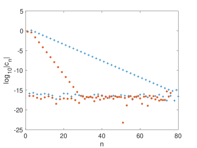
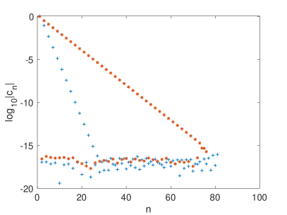
Figure 1. Chebyshev coefficients for the Peregrine solution given by ‘+’ in domain I and ‘*’ in domain II, on the left for $t=0$, on the right for $t=1$.

In Fig. 2 we show the $L^{\infty}$ norm of the difference between numerical and exact solution for $t=1$ in dependence of the number of time steps $N_{t}$. It can be seen that this is a fourth order method by comparing it to a straight line with slope $-4$ in the same figure. Below an accuracy of the order of $10^{-6}$ the convergence becomes slower than this since the conditioning of the Chebyshev differentiation matrices becomes important. This shows that numerical errors below $10^{-6}$ can be easily reached, but that for higher precisions the code from [4] based on an iterative approach has to be used. On the right of Fig. 2 we show the numerically computed quantity (14) in dependence of $N_{t}$. It shows a very similar behavior as the error $\Delta$ and is only slightly larger. Note that we cannot consider a relative error here since $E[u]$ (14) vanishes for the Peregrine solution.

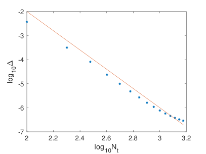
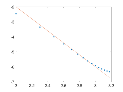
Figure 2. The $L^{\infty}$ norm of the difference between the numerical NLS solution for Peregrine initial data and the Peregrine solution for $t=1$ on the left, and the numerically computed $E[u]$ (14) on the right; the red line has in both cases slope $-4$.

3. Localized perturbations

In this section we consider localized perturbations of the Peregrine solution for the elliptic NLS equation ($\kappa=1$). Note that this equation does not play a role in the context of the water waves where only hyperbolic NLS equations are important, see the discussion in [23]. But the elliptic NLS equation plays a role in the context of nonlinear optics where the Peregrine solution has been recently observed in 1D, see [18]. It is also mathematically interesting.

Concretely we study the time evolution of the 2D elliptic NLS equation for the initial data

(15) $$u(x,y,0)=u_{Per}(x,0)+c\exp(-(x-x_{0})^{2}-y^{2})$$

with $c\in\mathbb{C}$ being a constant. We consider the 4 cases $x_{0}=0,-1$ and $c=\pm 0.1$. All examples are computed with $N_{I}=100$ and $N_{II}=101$ polynomials for the $x$-dependence, $N_{y}=2^{7}$ Fourier modes for $y=3[-\pi,\pi]$ and $N_{t}=1000$ time steps. Note that larger values of these parameters have only an effect on the solution below plotting accuracy, i.e., the resulting figures would be indistinguishable from the ones shown.

We first consider the case $x_{0}=-1$ and $c=0.1$ in Fig. 3, on the left the initial condition, on the right the solution for $t=0.5$. The solution is clearly unstable in the sense that the initial perturbations grow.

Figure 3. Solution to the 2D NLS equation for the initial data $u(x,y,0)=u_{Per}(x,t_{0})+0.1\exp(-(x+1)^{2}-y^{2})$ for $t=0$ on the left and $t=0.5$ on the right.

To show that the solution does not stay close to the Peregrine solution, we show in Fig. 4 the solutions for $t=0.5$ and for $y=0$ (minimal modulus of $u$ for $x=0$ and $t=0.5$) and $y=1.6199$ (one of the maxima of $|u|$ for $x=0$ and $t=0.5$) together with the Peregrine solution.

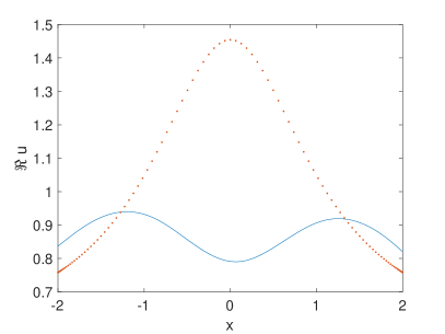
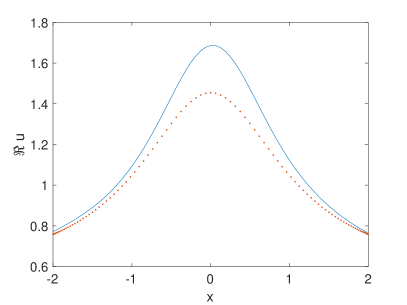
Figure 4. Real part of the solution to the 2D NLS equation for the initial data $u(x,y,0)=u_{Per}(x,t_{0})+0.1\exp(-(x+1)^{2}-y^{2})$ for $t=0.5$, on the left for $y=0$, on the right for $y=1.6199$; the Peregrine solution for the same time is shown as a dotted line.

The situation is similar in the case $x_{0}=-1$ and $c=-0.1$ as can be seen in Fig. 5: on the left the modulus of the solution for $t=0.5$ is shown, on the right the solution for $y=0$ together with the Peregrine solution (dotted). Again the perturbed solution does not stay close to the Peregrine solution.

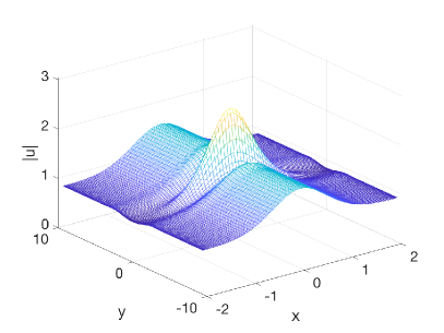
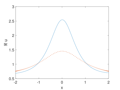
Figure 5. Solution to the 2D NLS equation for the initial data $u(x,y,0)=u_{Per}(x,t_{0})-0.1\exp(-(x+1)^{2}-y^{2})$ for $t=0.5$ on the left, and the real part of the solution at the same time for $y=0$ on the right together with the Peregrine solution (dotted).

The solution for the initial data (15) for $x_{0}=0$ and $c=0.1$ (on the left of Fig. 6) at time $t=0.5$ can be seen on the right of Fig. 6. The initial perturbations appear once more to grow in time.

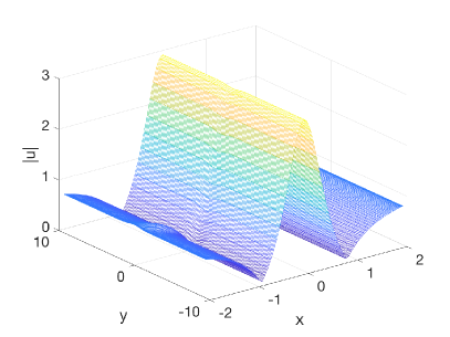
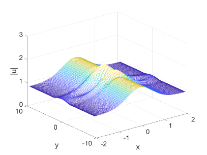
Figure 6. Solution to the 2D NLS equation for the initial data $u(x,y,0)=u_{Per}(x,t_{0})-0.1\exp(-(x-1)^{2}-y^{2})$ for $t=0$ on the left and $t=0.5$ on the right.

In Fig. 7 we show the solution on the right of Fig. 6 for $y=0$ and for $y=1.7671$, one of the maxima of the modulus of $u$ for $x=0$ together with the Peregrine solution.

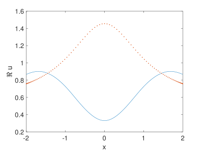
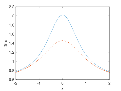
Figure 7. Real part of the solution to the 2D NLS equation for the initial data $u(x,y,0)=u_{Per}(x,t_{0})+0.1\exp(-x^{2}-y^{2})$ for $t=0.5$, on the left for $y=0$ and on the right for $y=1.7671$; the Peregrine solution for the same time is shown as a dotted line.

The situation changes somewhat in the case $x_{0}=0$ and $c=-0.1$. In this case the solution appears to blow up for $t\sim 0.49$ (the relative $E[u]$ conservation drops in this case below $10^{-3}$ and the code is stopped). The solution for $t=0.49$ can be seen on the left of Fig. 8. The $L^{\infty}$ norm of the solution in dependence of time on the right of the same figure also indicates a blow-up. This would imply that the Peregrine solution is strongly unstable as a solution to the 2D focusing elliptic NLS equation.

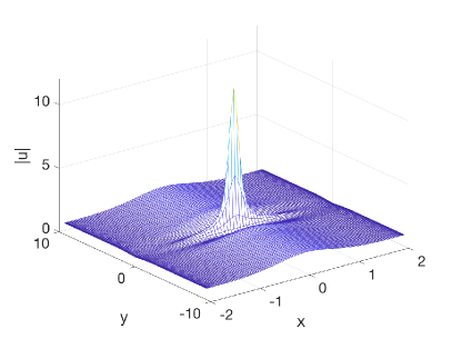
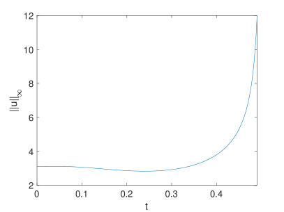
Figure 8. Solution to the 2D NLS equation for the initial data $u(x,y,0)=u_{Per}(x,t_{0})-0.1\exp(-x^{2}-y^{2})$ for $t=0.49$ on the left and the $L^{\infty}$ norm of the solution in dependence of time on the right.

4. Nonlocalized perturbations

In this section we study perturbations nonlocalized in $x$, but localized in $y$ of the Peregrine solution $u_{Per}$ of the form $u(x,t_{0})=(\sigma-\exp(-y^{2}))u_{Per}(x,t_{0})$, where $\sigma\sim 1$. The same numerical parameters as in the previous section are applied. We concentrate again on the elliptic case $\kappa=1$.

The solution for the case $\sigma=0.9$ (in Fig. 9 on the left) can be seen for $t=0.5$ in Fig. 9 on the right. Clearly the initial perturbations grow.

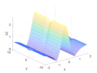
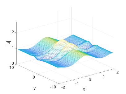
Figure 9. Solution to the 2D NLS equation for the initial data $(0.9-\exp(-y^{2}))u_{Per}(x,t_{0})$ for $t=0$ on the left and for $t=0.5$ on the right.

In Fig. 10 we show the solution on the right of Fig. 9 for $y=0$ and $y=2.0617$ (the maximum of the modulus of $|u|$) together with the dotted Peregrine solution. It can be seen that the perturbed NLS solution does not stay close to the latter.

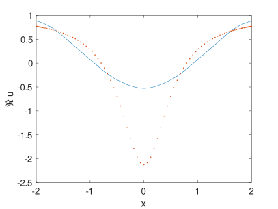
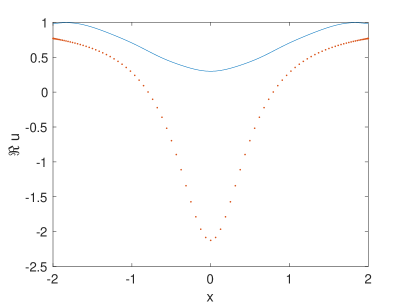
Figure 10. Real part of the solution to the 2D NLS equation for the initial data $(0.9-\exp(-y^{2}))u_{Per}(x,t_{0})$ for $t=0.5$ together with the dotted Peregrine solution, on the left for $y=0$, on the tight for $y=2.0617$.

The solution for the case $\sigma=1.1$ can be seen at different times in Fig. 11. The initial perturbation obviously grows, and the formed structures appear even to blow up in this case for $t\sim 0.4$.

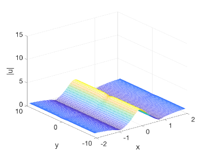
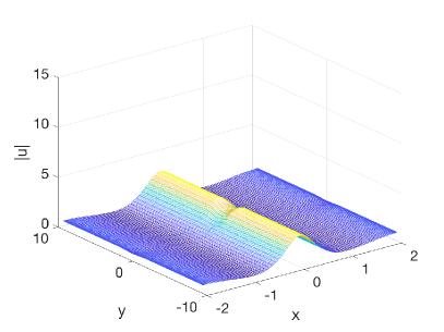
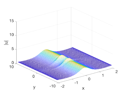
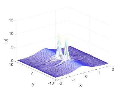
Figure 11. Solution to the 2D NLS equation for the initial data $(1.1-\exp(-y^{2}))u_{Per}(x,t_{0})$ for $t=0$, $t=0.134$, (left respectively right in the upper row), and $t=0.268$ and $t=0.4$ (left respectively right in the lower row).

A blow-up is suggested also by the $L^{\infty}$ norm of the solution which seemingly diverges as can be seen on the left of Fig. 12. The spectral coefficients on the right of the same figure also indicate a loss of resolution because of said blow-up.

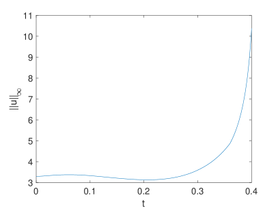
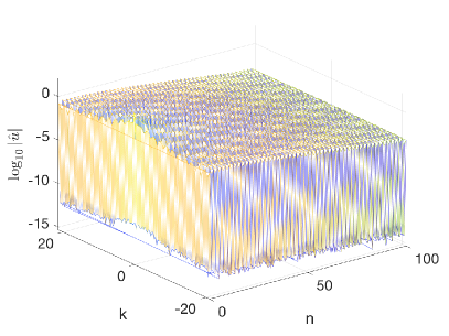
Figure 12. $L^{\infty}$ norm of the solution to the 2D NLS equation for the initial data $(1.1-\exp(-y^{2}))u_{Per}(x,t_{0})$ in dependence of $t$ on the left, and the spectral coefficients of the solution in domain I for the solution at $t=0.4$ on the right.

A blow-up once more suggests that the Peregrine solution is strongly unstable as a solution to the 2D focusing elliptic NLS equation. Whereas this is numerically difficult to decide, the solution is clearly unstable in the sense that it does not stay close to the exact solution at the same time as can be seen in Fig. 13, where the solution for two values of $y$ corresponding to the shown minimum $y=0$ and the maximum $y\sim 1.7671$ of $|u|$ in blue and the corresponding Peregrine solution in red is given.

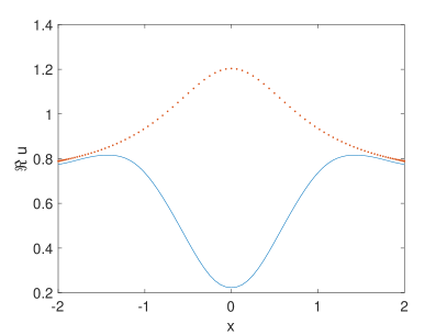
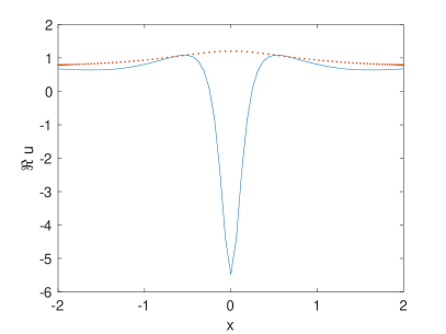
Figure 13. Real part of the solution to the 2D NLS equation for the initial data $(1.1-\exp(-y^{2}))u_{Per}(x,t_{0})$ in blue for $y=0$ the left, and for $y=1.7671$ on the right, and the respective Peregrine solution in red.

5. Hyperbolic nonlinear Schrödinger equation

In this section we study some of the examples of the previous sections in the context of the hyperbolic NLS equation. Since the Peregrine solution is again unstable against all considered perturbations, we concentrate on the localized perturbations (15) here, and show only the solution at the final time. No indication of blow-up is found in this case.

As detailed for instance in [23], hyperbolic NLS or Davey-Stewartson equations appear in the modulational regime of the water waves. Since the hyperbolic NLS equation has one focusing and one defocusing direction, no blow-up is to be expected in this case. Numerically this was confirmed in [21], for analytic results see [29]. The defocusing character of the $y$-direction implies that the numerical resolution is higher for the examples here (the Fourier coefficients in $y$ decrease to lower values), though we use the same numerical parameters as in section 3, where also plots of the initial configurations can be found.

As in Fig. 3 for the elliptic NLS equation, we first consider the case $x_{0}=-1$ and $c=\pm 0.1$ in (15). The solutions for $t=0.5$ are shown in Fig. 14. Again the perturbations do not disappear.

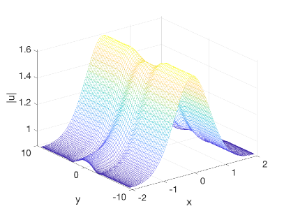
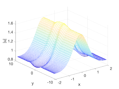
Figure 14. Solution to the hyperbolic NLS equation for the initial data $u(x,y,0)=u_{Per}(x,t_{0})\pm 0.1\exp(-(x+1)^{2}-y^{2})$ for $t=0.5$, on the left for the $+$ sign, on the right for the $-$ sign.

Of special interest is the situation of the initial data (15) for $x_{0}=0$ and $c=\pm 0.1$ since a blow-up was conjectured in the case with the $-$ sign, see Fig. 8. As can be seen in Fig. 15, there is no indication of a blow-up in this case for either sign of the initial data. The solution appears to be simply dispersed, but the initial perturbations do not decrease.

Figure 15. Solution to the hyperbolic NLS equation for the initial data $u(x,y,0)=u_{Per}(x,t_{0})\pm 0.1\exp(-x^{2}-y^{2})$ for $t=0.5$, on the left for the $+$ sign, on the right for the $-$ sign.

6. Conclusion

In this paper we have presented a numerical approach to the 2D cubic NLS equation (both in the elliptic and hyperbolic case) based on a multi-domain spectral approach with a compactified exterior domain in the $x$-coordinate (which allows to treat infinity as a finite point) and a Fourier spectral method in the coordinate $y$. This provides a spectral approach in both spatial coordinates which allows to achieve a numerical error exponentially decreasing with the resolution for functions periodic or rapidly decreasing in $y$ and rational and bounded at infinity in $x$. For the time integration a fully explicit fourth order method was presented based on a 4th order splitting scheme and an IRK4 method for the linear step.

This code allows to treat perturbations of the Peregrine solution with high precision and efficiency. In the examples studied the known instability of the Peregrine solution in 1D is shown to be amplified in 2D, also in the hyperbolic case which has one defocusing direction. All considered perturbations grow in time. In addition, numerical evidence for strong instability of the Peregrine solution in the elliptic case is presented: the solution appears to blow up in finite time if the initial data have an $E[u]$ (14) (which is finite on the considered torus in $y$) smaller than the one of the Peregrine solution.

It is left for a future project to develop better time integration schemes for the proposed spatial discretisation. An interesting approach would be to use exponential integrators as in [15, 14, 19] for which an efficient computation of matrix exponentials will be needed. In particular it will be necessary to filter the unphysical eigenvalues of the Chebyshev differentiation matrices, see the discussion in [30].

References

- [1] M.J. Ablowitz and T.P. Horikis, Interacting nonlinear wave envelopes and rogue wave formation in deep water, Physics of Fluids 27, 012107 (2015); https://doi.org/10.1063/1.4906770
- [2] H. Bailung, S. K. Sharma, and Y. Nakamura, Observation of Peregrine solitons in a multicomponent plasma with negative ions, Phys. Rev. Lett. 107, 255005 (2011).
- [3] J. Bérenger. A perfectly matched layer for the absorption of electromagnetic waves. J. Comput. Phys. 114, 185-200 (1994).
- [4] M. Birem and C. Klein, Multidomain spectral method for Schrödinger equations, Adv. Comp. Math. DOI 10.1007/s10444-015-9429-9 (2015)
- [5] J. Bona and J.-C. Saut, Dispersive Blow-Up II. Schrödinger-Type Equations, Optical and Oceanic Rogue Waves, Chinese Annals of Math. Series B, 31, (6), 793-810 (2010).
- [6] J.L. Bona, G. Ponce, J.-C. Saut, C. Sparber, Dispersive blow-up for nonlinear Schr dinger equations revisited, JMPA, 102, 782–811 (2014).
- [7] Boutet de Monvel, A., Fokas, A.S., Shepelsky, D.: Analysis of the global relation for the nonlinear Schro ?dinger equation on the half-line. Lett. Math. Phys. 65, 199 212 (2003)
- [8] A. Chabchoub, N. P. Hoffmann, and N. Akhmediev, Rogue wave observation in a water wave tank, Phys. Rev. Lett., 106, 204502 (2011).
- [9] A. Chabchoub, N. Hoffmann, M. Onorato, and N. Akhmediev, Super rogue waves: observation of a higher-order breather in water waves, Phys. Rev. X 2, 011015 (2012).
- [10] A. Chabchoub, N. Hoffmann, H. Branger, C. Kharif, and N. Akhmediev, Experiments on wind-perturbed rogue wave hydrodynamics using the Peregrine breather model, Physics of Fluids, 25, DOI: 10.1063/1.4824706 (2013).
- [11] A. Chabchoub, K. Mozumi, N. Hoffmann, A.V. Babanin, A. Toffoli, J.N. Steer, T.S. van den Bremer, N. Akhmediev, M. Onorato, and T. Waseda, Directional soliton and breather beams PNAS, 116 (20) 9759-9763, 2019.
- [12] P. Dubard, P. Gaillard, C. Klein, and V.B. Matveev, On multi-rogue wave solutions of the NLS equation and positon solutions of the KdV equation, Eur. Phys. J. Special Topics, 185, 247–258 (2010).
- [13] Grosch, C.E., Orszag, S.A.: Numerical solution of problems in unbounded regions: coordinate transforms. J. Comput. Phys. 25, 273 296 (1977)
- [14] M. Hochbruck and A. Ostermann, Exponential integrators, Acta Numerica (2010), pp. 209 286.
- [15] A.-K. Kassam and L. Trefethen, Fourth-Order Time-Stepping for stiff PDEs, SIAM J. Sci. Comput., 26 (2005), pp. 1214 1233.
- [16] T. Kato, Trotter’s product formula for an arbitrary pair of self-adjoint contraction semigroups, vol. 3, Academic Press, Boston, 1978, pp. 185 195.
- [17] U. Al Khawaja, H. Bahlouli, M. Asad-uz-zaman, S.M. Al-Marzoug, Modulational instability analysis of the Peregrine soliton, Commun Nonlinear Sci Numer Simulat 19, 2706 2714 (2014).
- [18] B. Kibler, J. Fatome, C. Finot, G. Millot, F. Dias, G. Genty, N. Akhmediev, and J. M. Dudley, The Peregrine soliton in nonlinear fibre optics, Nat. Phys. 6, 790–795 (2010).
- [19] C. Klein, Fourth order time-stepping for low dispersion Korteweg-de Vries and nonlinear Schrödinger equation, ETNA, 29, 116–135 (2008).
- [20] C. Klein and M. Haragus, Numerical study of the stability of the Peregrine breather, Annals of Mathematical Sciences and Applications, 2(2), 217-239 (2017).
- [21] C. Klein and J.-C. Saut, A numerical approach to Blow-up issues for Davey-Stewartson II type systems, Comm. Pure Appl. Anal. 14:4, 1443–1467 (2015)
- [22] C. Klein and N. Stoilov, A numerical study of blow-up mechanisms for Davey-Stewartson II systems, Stud. Appl. Math., DOI : 10.1111/sapm.12214 (2018)
- [23] D. Lannes, Water waves: mathematical theory and asymptotics, Mathematical Surveys and Monographs, vol 188 (2013), AMS, Providence.
- [24] Y.C. Li, On the so-called rogue waves in the nonlinear Schrödinger equation, preprint, arXiv:1511.00620v1 (2015)
- [25] F. Merle and P. Raphael. On universality of blow-up profile for l2 critical nonlinear Schrödinger equation. Inventiones Mathematicae, 156:565 672, 2004.
- [26] C. Muñoz, Instability in nonlinear Schrödinger breathers, Proyecciones Vol. 36, no. 4 (2017) 653 683.
- [27] D.H. Peregrine, Water waves, nonlinear Schrödinger equations and their solutions, J. Austral. Math. Soc. B, 25, 16–43, DOI:10.1017/S0334270000003891 (1983).
- [28] C. Sulem and P.L. Sulem. The nonlinear Schrödinger equation. Springer, 1999.
- [29] N. Totz, Global well-posedness of 2D non-focusing Schrödinger equations via rigorous modulation approximation, J. Dif. Equat. 261:2251 2299 (2016).
- [30] L. N. Trefethen, Spectral Methods in Matlab, SIAM, Philadelphia, PA, 2000.
- [31] H. Trotter, On the Product of Semi-Groups of Operators, Proceedings of the American Mathematical Society, 10 (1959), pp. 545 551.
- [32] Weideman, J.A.C. and Reddy, S.C., A Matlab differentiation matrix suite, ACM TOMS, 26 (2000), 465–519.
- [33] www.lorene.obspm.fr
- [34] H. Yoshida, Construction of higher Order symplectic Integrators, Physics Letters A, 150 (1990), pp. 262–268.
- [35] V.E. Zakharov and A.B. Shabat, Exact theory of two-dimensional self-focusing and one-dimensional selfmodulation of waves in nonlinear media. Sov. Phys. JETP, 34(1), 62–69 (1972); translated from Zh. Eksp. Teor. Fiz. 1, 118–134 (1971).
- [36] C. Zheng. A perfectly matched layer approach to the nonlinear Schrödinger wave equations. J. Comput. Phys. 227, 537-556 (2007).
- [37] C. Zheng, Exact nonreflecting boundary conditions for one-dimensional cubic nonlinear Schrödinger equations, J. Comput. Phys. 215, 552-565 (2006).