On resilience and connectivity of secure wireless sensor networks under node capture attacks

Abstract

Despite much research on probabilistic key predistribution schemes for wireless sensor networks over the past decade, few formal analyses exist that define schemes’ resilience to node-capture attacks precisely and under realistic conditions. In this paper, we analyze the resilience of the $q$-composite key predistribution scheme, which mitigates the node capture vulnerability of the Eschenauer–Gligor scheme in the neighbor discovery phase. We derive scheme parameters to have a desired level of resiliency, and obtain optimal parameters that defend against different adversaries as much as possible. We also show that this scheme can be easily enhanced to achieve the same “perfect resilience” property as in the random pairwise key predistribution for attacks launched after neighbor discovery. Despite considerable attention to this scheme, much prior work explicitly or implicitly uses an incorrect computation for the probability of link compromise under node-capture attacks and ignores real-world transmission constraints of sensor nodes. Moreover, we derive the critical network parameters to ensure connectivity in both the absence and presence of node-capture attacks. We also investigate node replication attacks by analyzing the adversary’s optimal strategy.

I Introduction

I-A Background

Wireless sensor networks (WSNs) deployed in hostile environments are subject to adversary attacks that can lead to sensor capture [17, 8, 7, 11]. Sensors are particularly vulnerable to such attacks because their physical protection is limited by low-cost considerations and their operation is unattended [11, 29, 7]. As a result of such attacks, all secret keys of a captured node are discovered by an adversary. Although random key predistribution schemes can be successfully used to secure communications in WSNs, they are often not explicitly designed to address node-capture vulnerabilities, and hence their resilience to such attacks is seldom analyzed formally. The main goal of this paper is to provide precise analytical results for resilience to node capture of one of the best known random key predistribution schemes, namely the $q$-composite extension of the basic Eschenauer and Gligor scheme [17] (hereafter referred to as the EG scheme), which was proposed by Chan et al. [8].

Background. The EG scheme [17], which is widely considered to be the basic random key predistribution mechanism, works as follows. For a WSN with $n$ nodes, in the key predistribution phase, a large key pool consisting of $P_{n}$ cryptographic keys is used to select uniformly at random $K_{n}$ distinct keys for each sensor node. These $K_{n}$ keys constitute the key ring of a sensor, and are installed in the sensor’s memory. After deployment, two sensors establish secure communication over an existing link if and only if their key rings have at least one key in common. Common keys are found in the neighbor discovery phase whereby a random constant is enciphered in all keys of a node and broadcast along with the resulting ciphertext block in a given area limited by the transmission power/range; i.e., in a local neighborhood. ${P}_{n}$ and $K_{n}$ are both functions of $n$ for generality, with the natural condition $1\leq K_{n}\leq P_{n}$.

According to the $q$-composite extension of the EG scheme [8], a secure link between two sensors is established if they share at least $q$ key(s) in their key rings, where $1\leq q\leq K_{n}$. Clearly, the $q$-composite scheme with $q=1$ reduces to the EG scheme. The $q$-composite scheme with $q\geq 2$ outperforms the EG scheme in terms of resilience (defined below) to small-scale sensor capture attacks while trading off increased vulnerability in the presence of large-scale attacks.

In addressing the resilience to node-capture attacks, we adopt the metric proposed by Chan et al. [8] where an adversary captures some random set of $m$ nodes. Communication between two arbitrary nodes, which are not among these $m$ nodes and have a secure communication link in between, may still be compromised (in particular be decrypted) by the adversary under the EG scheme and its $q$-composite version due to key collisions that can be generated during the predistribution phase. Thus, capturing nodes enables an adversary to compromise communications between non-captured nodes which happen to use keys that are also shared by captured nodes. We denote the probability of such compromise by $p_{\textnormal{compromised}}$ and, following Chan et al. [8], we say that a random key predistribution scheme is “perfectly resilient” to node-capture attacks if $p_{\textnormal{compromised}}=0$. This implies that only communications between a captured node and its direct neighbors are compromised in a perfectly resilient scheme. Hence, analysis of prefect resilience of a scheme must account for the number of neighbors of any captured node (e.g., minimum, average) to assess inherent vulnerability to node capture. Specifically, resilience analysis must explicitly address the connectivity property of a key graph arising from a key predistribution scheme under the classic disk model of communication [21, 22, 31, 12], which enables the computation of the number of neighbors of a captured sensor under realistic transmission constraints.

I-B Motivation

Why the $q$-composite scheme matters?

Although many key predistribution schemes have been proposed in the literature [5, 3, 14, 23, 15], we explain that the $q$-composite scheme matters as follows.

• Although there are other key predistribution schemes that by design are perfectly resilient after the neighbor discovery phase, the basic EG scheme and $q$-composite scheme can also be easily extended to be perfectly resilient after the neighbor discovery phase.

• Schemes are still vulnerable during the neighbor discovery phase, even being perfectly resilient after the neighbor discovery phase. In terms of resilience against node capture during the neighbor discovery stage, the $q$-composite scheme often outperforms the EG scheme and many other schemes.

We now discuss the above points ① and ② respectively. We look at ① first. Although the basic EG scheme and the $q$-composite scheme are not perfectly resilient, they can be easily extended to become perfectly resilient after neighbor discovery. For example, after the neighbor discovery phase of the EG scheme ends and two neighbor nodes identified by $ID_{i}$ and $ID_{j}$ discover that they share key $k_{ij}$, they can each compute a new shared key $K_{ij}=hash(ID_{i}||ID_{j}||k_{ij})$, where $i<j$ and $hash(\cdot)$ is a cryptographic hash function with pseudo-random output, and erase the old key $k_{ij}$. $K_{ij}$ is statistically unique (i.e., up to the birthday bounds) and hence the EG scheme becomes perfectly resilient by the above definition. Clearly, its $q$-composite version also becomes perfectly resilient if we include the uniquely ordered $q$ keys in the hash operation instead of the single key $k_{ij}$.

We now explain the above point ②. The $q$-composite scheme increases [8] the resilience of the EG scheme in the neighbor discovery phase where perfect resilience cannot hold; i.e., when $p_{\textnormal{compromised}}>0$. This is important since many random key predistribution schemes are also vulnerable to node capture in their neighbor-discovery phase even when they are perfectly resilient after neighbor discovery, and yet their vulnerabilities cannot be easily mitigated. For example, the random pairwise-key predistribution scheme of Chan et al. [8] is perfectly resilient and yet vulnerable to non-local communication compromise. In this scheme, prior to deployment, each sensor is matched up with a certain number of other randomly selected sensors. Then for each pair of sensors that are matched together, a pairwise key is generated and loaded in both sensors’ key rings. After deployment, any two nodes sharing a common pairwise key establish secure communication in the actual neighbor-discovery phase. Following neighbor discovery, each node erases its locally unused keys; i.e., keys that are shared with remote sensors located outside the transmission radius of a sensor. However, before these keys are erased, an adversary can capture and use them in his/her nodes strategically placed at various locations in the network to establish connections to sensors that are unreachable to remote legitimate neighbors; e.g., the adversary’s nodes can broadcast encrypted messages at these locations, find and connect to legitimate local sensor nodes.

Other pairwise predistribution schemes such as the ones by Liu and Ning [23] are constructed on a polynomial-based key predistribution protocol, while the scheme by Du et al. [15] is built on a threshold key exchange protocol. Both schemes exhibit the following threshold resilience property: after the adversary has captured some $m$ number of nodes, the fraction of compromised communications among non-captured nodes is close to $0$ for $m$ less than a certain threshold and sharply grows toward $1$ when $m$ surpasses the threshold. The larger $m$, the more sensor energy these schemes use for shared key generation. Thus, these schemes are not applicable in environments where $m$ is on the order of tens and hundreds of nodes. For this reason, threshold key predistribution schemes are less relevant to our analysis, despite their other interesting properties.

What are the limitations of prior work on the $q$-composite scheme in the literature?

Since the introduction of the $q$-composite scheme, it has received tremendous interest in the literature over the past decade [5, 3, 6, 23, 15]. However, prior researches have a few limitations which can be possibly addressed only via very recent advances. We discuss these limitations in terms of resiliency against node capture, network connectivity and replication attacks, respectively.

• Resilience against node capture in much prior studies: Incorrect analysis of link compromise. It was only recently discovered [33] that the computation of the probability of link compromise, $p_{\textnormal{compromised}}$, was incorrectly computed more than a decade ago by Chan et al. [8]. Hence, most prior work [23, 9, 31, 29, 30] used the incorrect computation either explicitly or implicitly, yielding inaccurate or even misleading results.

• Connectivity analysis in much prior studies: No consideration of transmission constraints, or relatively weak results when there is consideration. The analysis of resilience (even perfect resilience) of a scheme must account for the number of neighbors of any captured node to assess inherent vulnerability to node capture. Hence, resilience analysis must explicitly address connectivity of a key graph arising from key predistribution. This builds the connection between resilience and connectivity. In fact, connectivity analysis of the secure sensor network under key predistribution is also of significant virtue in its own because network-wide communication requires connectivity. Given the importance of network connectivity, there have been considerable studies on this issue [12, 2, 21, 22, 37]. However, few results address physical transmission constraints because considering both the security aspect (i.e., the key predistribution scheme) and transmission constraints will render the study much more challenging. Transmission constraints reflect real-world implementations of WSNs in which sensors have limited transmission capabilities so two remote sensors may not be able to communicate directly. Even under the classic disk model of communication where two sensors have to be within a certain distance from each other to communicate, connectivity analysis of secure sensor networks is difficult. Because of the difficulty, limited studies that consider secure connectivity under the disk model all present quite weak results. Note that the topology induced by the $q$-composite scheme is a key graph in which each of $n$ nodes selects $K_{n}$ number of keys uniformly at random from a common pool of $P_{n}$ keys, and two nodes establish an edge upon sharing at least $q$ keys (we denote the above key graph by $G_{q}(n,K_{n},P_{n})$). The disk model induces the so-called random geometric graph in which any two of $n$ uniformly distributed nodes on an area $\mathcal{A}$ have an edge in between if and only if their distance is at most some value, say $r_{n}$ (we denote the above random geometric graph $G_{RGG}(n,r_{n},\mathcal{A})$). Then the topology of a secure sensor network deploying the $q$-composite scheme under the disk model is given by the intersection of the key graph and the random geometric graph; i.e., a secure link exists only when the two nodes have an edge in the key graph and also have an edge in the random geometric graph. The reason is that a secure link between two sensors require them to share at least $q$ keys and also to be within distance $r_{n}$. For this graph intersection $G_{q}(n,K_{n},P_{n})\hskip 2.0pt{\cap}\hskip 2.0ptG_{RGG}(n,r_{n},\mathcal{A})$, due to the intertwining of the key graph and the random geometric graph, it is extremely difficult to obtain strong connectivity result. To illustrate the difficultly, we discuss a related yet simper problem that had been open for 18 years. Let us replace the key graph with a much simpler graph, the renowned Erdős–Rényi graph [16] $G_{ER}(n,p_{n})$, which is defined on $n$ nodes such that any two nodes establish an edge in between independently with the same probability $p_{n}$. This graph is much simpler than the key graph because it removes the edge dependencies [32]. Then we consider the graph intersection $G_{ER}(n,p_{n})\hskip 2.0pt{\cap}\hskip 2.0ptG_{RGG}(n,r_{n},\mathcal{A})$. After establishing connectivity result of $G_{RGG}(n,r_{n},\mathcal{A})$, Gupta and Kumar [20] in 1998 proposed a conjecture for connectivity of $G_{ER}(n,p_{n})\hskip 2.0pt{\cap}\hskip 2.0ptG_{RGG}(n,r_{n},\mathcal{A})$ (for the details of this conjecture, see Page I-D where we discuss related work). Despite many attempts to address this conjecture, it was resolved by Penrose [26] not until 2016. The difficulty is to analyze the connection structure when two distinct types of random graphs intersect: even individual graphs are highly connected, the resulting topology can become disconnected after intersection. We resolve an analog of the above conjecture for connectivity in $G_{q}(n,K_{n},P_{n})\hskip 2.0pt{\cap}\hskip 2.0ptG_{RGG}(n,r_{n},\mathcal{A})$, the intersection of the key graph and the random geometric graph. In particular, we show the connectivity has a sharp transition when the probability of a secure link is $\frac{\ln n}{n}$. To summarize, our strong connectivity result of the studied secure sensor network $G_{q}(n,K_{n},P_{n})\hskip 2.0pt{\cap}\hskip 2.0ptG_{RGG}(n,r_{n},\mathcal{A})$ is not obtained in the literature due to the difficulty of analyzing graph intersection. Prior results either ignore transmission constraints to analyze just the key graph, or consider the graph intersection but obtain relatively weak results (more details in Section I-D).

• Node-replication attacks in prior studies: Lack of formal or tractable analyses to determine the adversary’s optimal strategy. Although our main focus is to analyze node-capture resiliency and connectivity of the $q$-composite scheme, we also discuss node-replication attacks on the scheme (following Review 1’s suggestion). After node capture, the adversary can deploy replica nodes of compromised nodes by extracting keys from compromised nodes and then inserting some keys into the memory of replica nodes. Prior studies have investigated node-replication attacks, but most researches lacked formal analyses [24, 10, 38]. Limited studies have formally addressed node replication, but existing expressions to quantify node-replication attack are complex [19], making it intractable to determine the adversary’s optimal strategy to maximize node-replication attack given limited resource.

I-C Summary of Our Results

Our main results can be summarized as follows:

• We analyze the $q$-composite scheme’s resilience against node-capture attacks. We derive a tractable expression for the fraction of compromised communications under node capture, identify scheme parameters to have a desired level of resiliency, and obtain optimal parameters that defend against different adversaries as much as possible.

• We study connectivity of sensor networks with the $q$-composite scheme under real-world transmission constraints. We derive the critical conditions to guarantee secure network connectivity with high probability (i.e., with a probability converging to $1$ as the network size goes to infinity).

• For node-replication attacks, we investigate the adversary’s optimal strategy.

I-D Comparison with Related Work

We will first explain the improvements of this paper over related studies, and then discuss additional related work.

Improvement over prior work in terms of resiliency analysis against node capture. For a secure sensor network using the EG scheme [17] (i.e., the $q$-composite scheme with $q=1$), Di Pietro et al. [13, 14] prove that if $\frac{P_{n}}{K_{n}}=\Omega(n)$, the network is resilient in the sense that an adversary capturing sensors at random has to obtain at least a constant fraction of nodes of the network in order to compromise a constant fraction of secure links. We obtain the corresponding result for general $q$. Chan et al. [8] show that for the $q$-composite scheme, larger $q$ outperforms smaller $q$ in terms of resilience against small-scale sensor capture attacks while trading off increased vulnerability in the presence of large-scale attacks, but no analytical result that identifies the optimal $q$ is given. Furthermore, their computation is shown to be incorrect by Yum and Lee [33] recently. In contrast, we formally obtain optimal $q$ that defends against different adversaries as much as possible. Although Yum and Lee [33] have provided the correct expression to quantify node capture, but the expression is complex and intractable to analyze. We significantly simplify the expression via an asymptotic analysis, and this enables us to identify optimal scheme parameters.

Improvement over prior work in terms of connectivity analysis. Many studies on connectivity in secure sensor networks ignore real-world transmission constraints [12, 2, 8] because considering both the security aspect (i.e., the key predistribution scheme) and transmission constraints will render the analysis much more challenging. Because of the challenges, limited studies incorporating transmission constraints often present quite weak results [21, 22]. In the special case of $q=1$, Krzywdziński and Rybarczyk [22], and Krishnan et al. [21] recently show upper bounds $\frac{8\ln n}{n}$ and $\frac{2\pi\ln n}{n}$ for the critical threshold that the edge probability (i.e., the probability of a secure link between two sensors) takes for connectivity, while we prove the exact threshold as $\frac{\ln n}{n}$ for general $q$. The threshold is identified because we derive a sharp zero-one law for connectivity. Intuitively, a sharp zero–one law means that as the edge probability surpasses (resp., falls below) the critical value and grows (resp., declines) further, the network immediately becomes asymptotically connected (resp., disconnected). Chan and Fekri [9] approximate the key graph of the $q$-composite scheme by an Erdős–Rényi graph. However, there is a lack of rigorous argument for this approximation. A formal argument is needed because an Erdős–Rényi graph and a key graph used to represent the $q$-composite scheme are quite different; e.g., edges are all independent in the former but are not in the latter [32, 4, 36]. In this paper, we rigorously bridge these two graphs (we provide the details in Section VI of the full version [34] due to space limitation).

Improvement over prior work in terms of replication attack analysis. For node-replication attacks, prior researches either lack formal analyses [24, 10, 38], or provide intractable analyses [19]. We close this gap by presenting a simple asymptotic analysis, which further enables us to determine the adversary’s optimal strategy.

Other related studies. Key predistribution schemes by Liu and Ning [23] and Du et al. [15] have the threshold behavior: the probability of link compromise is close to $0$ under small-scale attacks but becomes close to $1$ after more than a threshold number of nodes are captured. Alarifi and Du [1] investigate data and code obfuscation techniques to improve resilience against node capture. Yang et al. [30] propose an approach of binding keys to geographic locations to improve the resilience against node capture. Defense mechanisms are also discussed by Vu et al. [29]. Conti et al. [11] introduce techniques to detect node-capture attacks. Bonaci et al. [7] apply control theory to model network behavior under node capture. Tague and Poovendran [28] evaluate node-capture attacks in sensor networks by decomposing them into collections of primitive events.

Erdős and Rényi [16] analyze connectivity in the classical Erdős–Rényi graph [16] $G_{ER}(n,p_{n})$ (the graph is named after them), while Gupta and Kumar [20] address a random geometric graph $G_{RGG}(n,r_{n},\mathcal{A})$. Both studies show that a critical threshold of connectivity in either graph is that the edge probability equals $\frac{\ln n}{n}$; i.e., $G_{ER}(n,p_{n})$ is connected (resp., disconnected) if $p_{n}\sim\frac{a\ln n}{n}$ for some constant $a>1$ (resp., some constant $a<1$), while $G_{RGG}(n,r_{n},\mathcal{A})$ is connected (resp., disconnected) if $\pi{r_{n}}^{2}\sim\frac{a\ln n}{n}$ for some constant $a>1$ (resp., some constant $a<1$). Gupta and Kumar [20] conjecture that the intersection $G_{ER}(n,p_{n})\hskip 2.0pt{\cap}\hskip 2.0ptG_{RGG}(n,r_{n},\mathcal{D})$ will also have a similar connectivity result where a critical threshold of connectivity is that the edge probability $\pi{r_{n}}^{2}p_{n}$ equals $\frac{\ln n}{n}$. Despite the seemingly simple extension, the Gupta–Kumar conjecture had been open for 18 years (1998–2016) before being confirmed by Penrose’s recent ground-breaking work [26].

I-E Organization and Notation

Roadmap. The rest of the paper is organized as follows. We introduce useful notation below. In Section II, we analyze the resilience of the $q$-composite scheme against node capture. Section III presents connectivity results of a sensor network under the $q$-composite scheme, in consideration of sensors’ limited transmission ranges. We quantify node-replication attacks in Section IV. Section V provides analytical details for resilience. We conclude the paper in Section VI.

Notation. Throughout the paper, $q$ is an arbitrary positive integer and does not scale with $n$, the number of nodes in the sensor network. We define $p_{s}$ as the probability that the key rings of two sensors share at least $q$ keys in the $q$-composite scheme, where the subscript “s” means “secure”. $p_{s}$ is a function of the parameters $K_{n},P_{n}$ and $q$. All limits are taken with $n\to\infty$. We use the standard asymptotic notation $o(\cdot),O(\cdot),\omega(\cdot),\Omega(\cdot),\Theta(\cdot)$ and $\sim$; see [35, Page 2-Footnote 1]. In particular, for two positive sequences $x_{n}$ and $y_{n}$, the relation $x_{n}\sim y_{n}$ signifies $\lim_{n\to\infty}(x_{n}/y_{n})=1$.

II Resilience of $q$-Composite Scheme
against Node Capture

We now rigorously evaluate the resilience against node capture in sensor networks employing the $q$-composite scheme. We consider the case where the adversary has captured some random set of $m$ nodes. Throughout the rest of the paper, we let $p_{\textnormal{compromised}}$ denote the probability that secure communication between two non-captured nodes is compromised by the adversary (we often refer to this probability as probability of link compromise). Due to node homogeneity, $p_{\textnormal{compromised}}$ is also the fraction of compromised communications among non-captured nodes. In the work proposing the $q$-composite scheme, Chan et al. [8] have already computed $p_{\textnormal{compromised}}$. Unfortunately, this computation, cited in numerous following studies [9, 23, 31, 29, 30], is shown to be incorrect by Yum and Lee [33] recently. Both the incorrect and correct formulas are quite involved, so we defer presenting them to Section V-A. Given the correct yet complex formula, it is still challenging to interpret how $p_{\textnormal{compromised}}$ varies with respect to the parameters. To this end, we significantly simplify $p_{\textnormal{compromised}}$ via an asymptotic analysis, and this enables us to identify scheme parameters to have a desired level of resiliency, and to choose optimal parameters that defend against different adversaries as much as possible. The intuition of our analysis is that although $p_{\textnormal{compromised}}$ is complex for finite $n$, we manage to derive simple asymptotic result of $p_{\textnormal{compromised}}$. Despite simple asymptotics obtained, the analysis to derive the result turns out to be non-trivial since it involves significant simplification of a complex expression.

II-A Summary of Results

We now summarize the main results formally. First, we identify the condition for negligible probability of link compromise, where a probability is negligible if it converges to $0$ as $n\to\infty$.

Theorem 1 (Conditions for negligible probability of link compromise).

The probability $p_{\textnormal{compromised}}$ of link compromise is negligible if $m\Big{/}\big{(}\frac{P_{n}}{K_{n}}\big{)}$ is negligible. In other words, if

$$m=o\bigg{(}\frac{P_{n}}{K_{n}}\bigg{)},$$ (1)

then $p_{\textnormal{compromised}}=o(1).$

Intuitively, Theorem 1 exhibits the following finding: to compromise a constant fraction of communication links between non-captured nodes in the network, the adversary has to capture at least some number of nodes such that these nodes combined have a number of keys at least a constant fraction of the key pool. An immediate implication of Theorem 1 gives the condition of scheme parameters to have a desired level of resiliency: the adversary has to capture a constant fraction of nodes in order to compromise a constant fraction of communication links in the network. Specifically, we obtain Corollary 1 below.

Corollary 1 (Scheme condition to achieve desired resiliency).

If

$$\frac{P_{n}}{K_{n}}=\Omega(n),$$ (2)

then the network has a desired level of resilience against node capture in the sense that the adversary has to capture a constant fraction of nodes in order to compromise a constant fraction of communication links in the network. Put formally, we have $p_{\textnormal{compromised}}=o(1)$ if $m=o(n)$.

Theorem 1 above provides condition for $p_{\textnormal{compromised}}=o(1)$, but there is no detailed expression of $p_{\textnormal{compromised}}$. This is given by Theorem 2 below, which establishes the asymptotically exact probability of link compromise. Theorem 2 will enable to us to optimize scheme parameters to defend against different attackers.

Theorem 2 (Asymptotic probability of link compromise).

Let the notation “$\sim$” denote asymptotic equivalence. Specifically, for two positive sequences $x_{n}$ and $y_{n}$, the relation $x_{n}\sim y_{n}$ means $\lim_{n\to\infty}(x_{n}/y_{n})=1$. We also define $p_{s}$ as the probability that the key rings of two sensors share at least $q$ keys. If

$$m=o\bigg{(}\sqrt{\frac{P_{n}}{{K_{n}}^{2}}}\hskip 2.0pt\bigg{)},$$ (3)

and

$$K_{n}=\omega(1),$$ (4)

then

$$p_{\textnormal{compromised}} \sim\bigg{(}\frac{mK_{n}}{P_{n}}\bigg{)}^{q},$$ (5)

and

$$\frac{p_{\textnormal{compromised}}}{p_{s}} \sim q!\bigg{(}\frac{m}{K_{n}}\bigg{)}^{q}.$$ (6)

Now we use Theorem 2 for optimizing scheme parameters to defend against different adversaries. In particular, we will consider two different adversaries and show how to choose the key-sharing requirement $q$ (two sensors should share at least $q$ keys in order to establish a secure link in between).

To see the impact of $q$ on node-capture attacks, we will fix the key ring size $K_{n}$ and the key-setup probability $p_{s}$. This means that the key pool size $P_{n}$ needs to decrease as $q$ increases. We first consider an adversary who has captured a certain number of nodes, $m$. In other words, given $m$, we study how $p_{\textnormal{compromised}}$ varies with respect to $q$. The result is that there exists an optimal $q$ to minimize $p_{\textnormal{compromised}}$ for an adversary that has captured $m$ nodes. More specifically, we have the following Corollary 2.

Corollary 2 (Minimizing link compromise with respect to $q$ given the number of captured nodes).

To minimize the fraction of communications compromised by an adversary who has captured $m$ nodes, the optimal $q$ is $q^{*}=\max\{\big{\lfloor}\frac{K_{n}}{m}\big{\rfloor},1\}$; i.e., $q^{*}=\big{\lfloor}\frac{K_{n}}{m}\big{\rfloor}$ if $\frac{K_{n}}{m}>1$, and $q^{*}=1$ if $\frac{K_{n}}{m}\leq 1$, where the floor function $\lfloor x\rfloor$ maps a real number $x$ to the largest integer that is no greater than $x$.

We then consider an adversary whose goal is to compromise a certain fraction of communications. We show that there exists an optimal $q$ to maximize the number of nodes needed to be captured by such an adversary (again, the key ring size $K_{n}$ and the key-setup probability $p_{s}$ are both fixed). More specifically, we present Corollary 3 below.

Corollary 3 (Maximizing needed node capture with respect to $q$ given the fraction of link compromise).

To maximize the resource (specifically, to maximize the number of captured nodes) needed for an adversary whose goal is to compromise $p_{\textnormal{compromised}}$ fraction of communications, the optimal $q$ is the solution $q^{\#}$ to maximize $(\frac{p_{\textnormal{compromised}}/p_{s}}{q!})^{1/q}$. The solution $q^{\#}$ is difficult to derive formally, but can given empirically by Table I and illustrated by Figure 1. The above result is obtained by proving that the number of captured nodes needed to compromise $p_{\textnormal{compromised}}$ fraction of communications equals $K_{n}\times(\frac{p_{\textnormal{compromised}}/p_{s}}{q!})^{1/q}$ asymptotically.

TABLE I: This table presents the relationship between $\frac{p_{\textnormal{compromised}}}{p_{s}}$ and $q^{\#}$ which maximizes $(\frac{p_{\textnormal{compromised}}/p_{s}}{q!})^{1/q}$.

$\frac{p_{\textnormal{compromised}}}{p_{s}}$	$[0.5,\infty)$	$[0.222,0.5]$	$[0.094,0.222]$	$[0.038,0.094]$	$[0.016,0.038]$
$q^{\#}$ (i.e., optimal $q$)	1	2	3	4	5

$\frac{p_{\textnormal{compromised}}}{p_{s}}$	$[0.0053,0.016]$	$[0.0023,0.0053]$	$[0.0009,0.0023]$	$\ldots$
$q^{\#}$ (i.e., optimal $q$)	6	7	8	$\ldots$

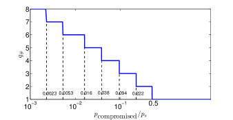
Figure 1: The plot of $q^{\#}$ with respect to ${p_{\textnormal{compromised}}/p_{s}}$, where $q^{\#}$ maximizes $(\frac{p_{\textnormal{compromised}}/p_{s}}{q!})^{1/q}$.

All of our results above will be proved in Section V-D. We now discuss Theorem 2 in particular since it has a set of seemingly complex conditions. Results other than Theorem 2 are less involved and have already been well explained.

II-B Further Explanations of Theorem 2

We will interpret conditions and results of Theorem 2 for a better understanding.

Interpreting (3) (i.e., $m=o\big{(}\sqrt{\frac{P_{n}}{{K_{n}}^{2}}}\hskip 2.0pt\big{)}$). To provide a more intuitive understanding, we discuss (3) below. To compute the probability $p_{\textnormal{compromised}}$ of link compromise under $m$ captured nodes, Bayes’ rule is used by considering the number of different keys in the key rings of the $m$ captured nodes. Specifically, after $A_{\tau}$ denotes the probability that the $m$ captured nodes have $\tau$ different keys in total, and $B_{\tau}$ denotes the conditional probability of link compromise conditioning on the event that the $m$ captured nodes have $\tau$ different keys in total, it is straightforward from Bayes’ rule that $p_{\textnormal{compromised}}=\sum_{\tau}(A_{\tau}B_{\tau})$, where $\tau$ iterates its possible values; i.e., $K_{n}\leq\tau\leq\min\{mK_{n},P_{n}\}$, which holds from the following three points. First, $A_{\tau}$ is at least $K_{n}$ because each node already has $K_{n}$ keys. Second, $A_{\tau}$ may take the maximum $mK_{n}$ when the key rings of the $m$ captured nodes are completely different. Third, an additional note is that the above maximum cannot exceed $P_{n}$ since the whole key pool has $P_{n}$ keys. Now that given $p_{\textnormal{compromised}}=\sum_{\tau}(A_{\tau}B_{\tau})$, because $A_{\tau}$ and $B_{\tau}$ have complex expressions, it makes difficult for us to understand how $p_{\textnormal{compromised}}$ changes with respect to network parameters and how we can choose parameters to minimize $p_{\textnormal{compromised}}$. In order to simplify computing $p_{\textnormal{compromised}}$, we want to provide a simple yet rigorous approximation. To start with, we consider the distribution of $\tau$, the number of different keys in the key rings of the $m$ captured nodes. Since we are mostly concerned with the practical case where the key pool size $P_{n}$ is much larger than the key ring size $K_{n}$ and the captured-node number $m$, it is reasonable to consider that the key rings of the $m$ captured nodes are completely different so that $\tau=mK_{n}$. We want to ensure this event with high probability; i.e., the probability $A_{mK_{n}}$ of this event can be written as $1-o(1)$ (arbitrarily close to $1$ for large $n$). If $A_{mK_{n}}=1-o(1)$, then any $A_{\tau}$ with $\tau<mK_{n}$ will be $o(1)$ (i.e., negligible) since all $A_{\tau}$ sums to $1$. In addition, clearly $B_{\tau}$ increases as $\tau$ increases because link compromise is more likely conditioning on that the $m$ captured nodes have more different keys in total. Given the above, if $A_{mK_{n}}=1-o(1)$, recalling $p_{\textnormal{compromised}}=\sum_{\tau}(A_{\tau}B_{\tau})$, we can use $A_{mK_{n}}B_{mK_{n}}$ and furthermore $B_{mK_{n}}$ to approximate $p_{\textnormal{compromised}}$. Evaluating $B_{mK_{n}}$ is much simpler than computing all $A_{\tau}$ and $B_{\tau}$, and we defer the discussion of $B_{mK_{n}}$ next. Note that here our explanation is intuitive (sometimes not rigorous), but we present a rigorous analysis in Section V.

Now we return to how we can find a condition to ensure $A_{mK_{n}}=1-o(1)$. The probability $A_{mK_{n}}$ is the event that after each captured node selects $K_{n}$ keys uniformly at random from the key pool of $P_{n}$ keys, the total number of different keys selected equals $mK_{n}$. We first discuss a simple intuition using the renowned “birthday paradox” [27]. In “birthday paradox”, each of $m$ persons has a birthday selected randomly from a year (say $P$ days), then it is well known that if $m$ is on the order of $\sqrt{P}$, at least two people celebrate the same birthday with high probability; in contrast, if $m$ is much smaller than $\sqrt{P}$, all people have different birthdays with high probability. This “birthday paradox” example corresponds to the special case of key distribution where each node selects just one key from the key pool (note that the notions of node and key correspond to person and birthday). Hence, if $K_{n}$ is just $1$, we know from the “birthday paradox” that if $m$ is much smaller than $\sqrt{P_{n}}$, all $m$ captured nodes will have different keys with high probability. Now for the general case where $K_{n}$ is not $1$, the intuition thus becomes that if $mK_{n}$ is much smaller than $\sqrt{P_{n}}$ (formally $mK_{n}=o(\sqrt{P_{n}})$), all $m$ captured nodes will have different keys with high probability. In fact, this can also be seen from a simple analysis. Without any restriction, there are $\binom{P_{n}}{K_{n}}$ ways to construct a key ring of each node, and thus $\left[\binom{P_{n}}{K_{n}}\right]^{m}$ ways to construct the key rings of $m$ nodes. Now for the case where $m$ captured nodes together have $mK_{n}$ different keys, there are $\binom{P_{n}}{K_{n}}\binom{P_{n}-K_{n}}{K_{n}}\ldots\binom{P_{n}-(m-1)K_{n}}{K_{n}}$ ways to construct the key rings, since the first node has $\binom{P_{n}}{K_{n}}$ choices, the second node has $\binom{P_{n}-K_{n}}{K_{n}}$ choices in order to not share any key with the first node, and so on. Then $A_{mK_{n}}$ can be given by $\frac{\prod_{j=0}^{m-1}\binom{P_{n}-jK_{n}}{K_{n}}}{\left[\binom{P_{n}}{K_{n}}\right]^{m}}$, and the result $A_{mK_{n}}=1-o(1)$ under $mK_{n}=o(\sqrt{P_{n}})$ can be formally proved. The above condition $mK_{n}=o(\sqrt{P_{n}})$ is precisely (3) after simple arrangements.

To summarize, we introduce (3) so that the $m$ captured nodes together will have $mK_{n}$ different keys with high probability and then we only need to conditioning on this event to provide a rigorous approximation for the probability of link compromise.

Interpreting (5) (i.e., $p_{\textnormal{compromised}}\sim\big{(}\frac{mK_{n}}{P_{n}}\big{)}^{q}$). We have explained above that the $m$ captured nodes together will have $mK_{n}$ different keys with high probability so that $p_{\textnormal{compromised}}=\sum_{\tau}(A_{\tau}B_{\tau})$ can be approximated by $B_{mK_{n}}$, where $B_{mK_{n}}$ is the probability of event $\mathcal{B}_{mK_{n}}$, with $\mathcal{B}_{mK_{n}}$ denoting the event of link compromise conditioning on the event that the $m$ captured nodes have $mK_{n}$ different keys in total. We now analyze $B_{mK_{n}}$ by Bayes’ rule. Let $C_{mK_{n},u}$ denotes the probability of event $\mathcal{B}_{mK_{n}}$ conditioning on the event that two benign nodes share $u$ keys in their key rings. Recall that $p_{s}$ is the probability that two benign nodes share at least $q$ keys in their key rings (i.e., $p_{s}$ is the link-setup probability in the $q$-composite scheme), and $\rho_{u}$ denotes the probability that two benign nodes share exactly $u$ keys in their key rings. Given there is already a link between two benign nodes, the probability that they share exactly $u$ keys is $\frac{\rho_{u}}{p_{s}}$. Given the above, we obtain from Bayes’ rule that $B_{mK_{n}}=\sum_{u=q}^{K_{n}}(C_{mK_{n},u}\cdot\frac{\rho_{u}}{p_{s}})$. In our studied parameter range, $\frac{\rho_{q}}{p_{s}}$ is much greater than $\frac{\rho_{u}}{p_{s}}$ with $u>q$; i.e., given there is already a link between two benign nodes, then it is most likely that they share exactly $q$ keys rather than more than $q$ keys. Hence, we only need to evaluate link compromise in the case where the two benign nodes share exactly $q$ keys. Without any restriction, there are $\binom{P_{n}}{q}$ to select these $q$ keys. To compromise this link, these $q$ keys must fall into the $mK_{n}$ keys that the $m$ captured nodes together have, and there are $\binom{mK_{n}}{q}$ choices to select the $q$ keys. Then the link compromise probability becomes $\frac{\binom{mK_{n}}{q}}{\binom{P_{n}}{q}}$, whose numerator and denominator become roughly $\frac{1}{q!}(mK_{n})^{q}$ and $\frac{1}{q!}{P_{n}}^{q}$ respectively for $mK_{n}$ and $P_{n}$ much greater than $q$. Then we finally obtain the expression $\big{(}\frac{mK_{n}}{P_{n}}\big{)}^{q}$ for $p_{\textnormal{compromised}}$; i.e., (5) follows.

Interpreting (4) (i.e., $K_{n}=\omega(1)$). We need $K_{n}=\omega(1)$ so that $\binom{mK_{n}}{q}$ above becomes $\frac{1}{q!}(mK_{n})^{q}$ asymptotically.

Interpreting (6) (i.e., $\frac{p_{\textnormal{compromised}}}{p_{s}}\sim q!\big{(}\frac{m}{K_{n}}\big{)}^{q}$). We have already interpreted (5) (i.e., $p_{\textnormal{compromised}}\sim\big{(}\frac{mK_{n}}{P_{n}}\big{)}^{q}$) above. Then (6) (i.e., $\frac{p_{\textnormal{compromised}}}{p_{s}}\sim q!\big{(}\frac{m}{K_{n}}\big{)}^{q}$) follows from (5) and (35) on Page 35 (i.e., $p_{s}\sim\frac{1}{q!}\big{(}\frac{{K_{n}}^{2}}{P_{n}}\big{)}^{q}$).

II-C Practicality of the Conditions in the Results

We check the practicality of (2). Recall that $n$ is the number of sensors, the key ring size $K_{n}$ controls the number of keys in each sensor’s memory and $P_{n}$ is the key pool size. In real-world implementations of sensor networks, $K_{n}$ is several orders of magnitude smaller than $P_{n}$ and $n$ due to limited memory and computational capability of sensors, and $P_{n}$ is larger [17, 8, 31] than $n$. Therefore, (2) is practical. In fact, Di Pietro et al. [14] also consider the range of $\frac{P_{n}}{K_{n}}=\Omega(n)$ in the special case of $q=1$. In addition, under (2) and a reasonable assumption that only a small number (in particular $o(n)$) of sensors are captured by the adversary, (1) follows since any $o(n)$ can be expressed as $o\big{(}\frac{P_{n}}{K_{n}}\big{)}$ by (2).

For $m\geq 1$, condition (3) implies $\frac{P_{n}}{{K_{n}}^{2}}=\omega(1)$; i.e., $\frac{{K_{n}}^{2}}{P_{n}}=o(1)$. We check the practicality of (4) (i.e., $K_{n}=\omega(1)$) and $\frac{{K_{n}}^{2}}{P_{n}}=o(1)$. Since $K_{n}$ is often larger than $\ln n$ in real-world implementations [31, 36], the practicality of $K_{n}=\omega(1)$ follows. As mentioned, $P_{n}$ is much larger compared to $K_{n}$, so $\frac{{K_{n}}^{2}}{P_{n}}=o(1)$ also holds in practice. In addition, to have an idea of $m$ in (3), we observe $K_{n}$ is much less than $n$ and $P_{n}$ is larger (but not too much) than $n$ [17, 8, 31], so $\sqrt{\frac{P_{n}}{{K_{n}}^{2}}}$ in (3) is often a fractional order of $n$. Under small-scale node-capture attacks, $m$ satisfies (3).

II-D Experiments

We provide experiments to confirm our theoretical results.

II-D1 Impact of scheme parameters to link compromise by an adversary with a given number of captured nodes

We present Figures 2 and 3 on Page 3 to illustrate the impact of scheme parameters to link compromise by an adversary with a given number of captured nodes. Each figure has four subfigures. In each subfigure, we fix $K$ and $p_{s}$, and study how $p_{\textnormal{compromised}}$ changes with respect to $q$ for different $m$ (we often write $K_{n}$ and $P_{n}$ as $K$ and $P$ when not considering their scalings with $n$). Across subfigures of either Figure 2 or 3, we consider different $K$, and across some subfigures, we also have different sets of $m$ for better discussion (explained soon). Between Figures 2 and 3, we consider different $p_{s}$. Hence, our experiments and the resulting figure plots provide a comprehensive study to validate our theoretical results.

In all 8 subfigures, we observe that:

• for each curve, $p_{\textnormal{compromised}}$ is indeed minimized at $q=\max\{\big{\lfloor}\frac{K}{m}\big{\rfloor},1\}$, which confirms Corollary 2.

For the above point, our plots address the case of $\big{\lfloor}\frac{K}{m}\big{\rfloor}$ being an integer (e.g., $K=40$ with $m=40,20,10$ in Figure 2) as well as the case where $\big{\lfloor}\frac{K_{n}}{m}\big{\rfloor}$ is not an integer (e.g., $K=80$ with $m=30$ in Figure 2, and $K=120$ with $m=50$ in Figure 2). For this reason, some subfigures have different sets of $m$. Furthermore, as explained below, we find that the plots are in agreement with our asymptotic result (6) (i.e., $\frac{p_{\textnormal{compromised}}}{p_{s}}\sim q!\big{(}\frac{m}{K_{n}}\big{)}^{q}$):

• Given $q$, $K$ and $p_{s}$, $p_{\textnormal{compromised}}$ increases with $m$. This can be seen from that in each subfigure, curves with larger $m$ are always above curves with lower $m$.

• Given $q$, $m$ and $p_{s}$, $p_{\textnormal{compromised}}$ decreases with $K$. This can be seen from that for either Figure 2 or 3, from subfigure (a) to (d), the curves become lower and lower as $K$ increases (we compare curves with the same $m$).

• Given $q$, $K$ and $m$, $p_{\textnormal{compromised}}$ increases with $p_{s}$, This can be seen from that the curves in Figure 2 (resp., (b) (c) (d)) are lower than those of Figure 3 (resp., (b) (c) (d)) (we compare curves with the same $m$).

II-D2 Impact of scheme parameters to the required number of captured nodes by an adversary with a given fraction of link compromise as its goal

We further present Figure 4 on Page 3 to illustrate the impact of scheme parameters to the required number of captured nodes by an adversary whose goal is to compromise a given fraction of links. Figure 4 has four subfigures. In each subfigure, we fix $K$ and $p_{s}$, and study how $m$ changes with respect to $q$ for different $p_{\textnormal{compromised}}$. Between subfigures (a) and (b) of Figure 4, we consider different $p_{s}$ with the same $K$ and the same set of $p_{\textnormal{compromised}}$. Compared with subfigures (a) and (b), we then consider a partially different set of $p_{\textnormal{compromised}}$ as well as different $p_{s}$ in Figure 4. We further look at a different $K$ in Figure 4. Hence, our experiments here also provide a comprehensive study.

In all 4 subfigures, we observe that:

• for each curve, $m$ is maximized at Corollary 3’s $q^{\#}$, which is determined by Table I or Figure 1 on Page I given $\frac{p_{\textnormal{compromised}}}{p_{s}}$.

From Corollary 3, $m$ denoting the number of captured nodes needed to compromise $p_{\textnormal{compromised}}$ fraction of communications equals $K\times(\frac{p_{\textnormal{compromised}}/p_{s}}{q!})^{1/q}$ asymptotically. Then

• Given $K$ and $p_{s}$, $m$ increases with $p_{\textnormal{compromised}}$. This can be seen from that in each subfigure, curves with larger $p_{\textnormal{compromised}}$ are always above curves with lower $p_{\textnormal{compromised}}$.

• Given $K$ and $p_{\textnormal{compromised}}$, $m$ decreases with $p_{s}$. This can be seen from that between subfigures (a) and (b) of Figure 4, the curves become lower as $p_{s}$ increases (we compare curves with the same $p_{\textnormal{compromised}}$).

• Given $p_{s}$ and $p_{\textnormal{compromised}}$, $m$ decreases with $K$. This can be seen from that between subfigures (a) and (c) of Figure 4, the curves become higher as $K$ increases (we compare curves with the same $p_{\textnormal{compromised}}$).

Summarizing ①–⑧ above, we conclude that the experiments are in accordance with our theoretical findings.

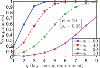
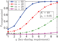
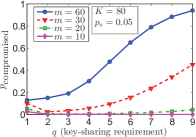
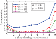
Figure 2: Each subfigure plots the fraction of compromised communications between non-captured nodes, $p_{\textnormal{compromised}}$, with respect to $q$ when $m$ nodes are captured, and we fix $K$ and $p_{s}$ in each subfigure. In different subfigures, we have different $K$ and fix $p_{s}$ as $0.05$. We observe that the $q$ that minimizes $p_{\textnormal{compromised}}$ is in accordance with Corollary 2; more specifically, the optimal $q$ is $\max\{\big{\lfloor}\frac{K_{n}}{m}\big{\rfloor},1\}$, where the floor function $\lfloor x\rfloor$ maps a real number $x$ to the largest integer that is no greater than $x$.

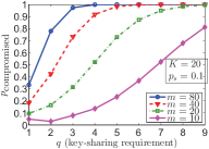
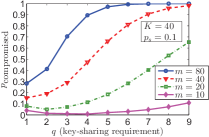
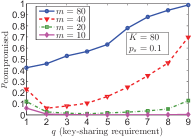
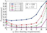
Figure 3: Each subfigure plots the fraction of compromised communications between non-captured nodes, $p_{\textnormal{compromised}}$, with respect to $q$ when $m$ nodes are captured, and we fix $K$ and $p_{s}$ in each subfigure. In different subfigures, we have different $K$ and fix $p_{s}$ as $0.1$. Similar to Figure 2 above, we see that the $q$ that minimizes $p_{\textnormal{compromised}}$ is $\max\{\big{\lfloor}\frac{K_{n}}{m}\big{\rfloor},1\}$ and thus in agreement with Corollary 2.

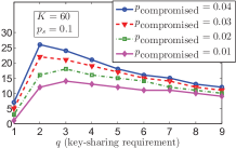
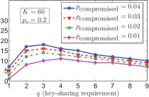
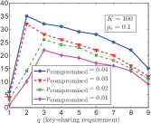
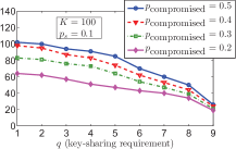
Figure 4: The $y$ axis stands for the number of nodes to be captured to ensure $p_{\textnormal{compromised}}$ fraction of compromised communications between non-captured nodes. In each subfigure, different lines have different $p_{\textnormal{compromised}}$, while different points in each line vary $q$ while fixing $K$ and $p_{\textnormal{compromised}}$. We observe that the $q$ that maximizes $m$ is in accordance with Corollary 3; more specifically, given $\frac{p_{\textnormal{compromised}}}{p_{s}}$, the optimal $q$ is determined by Table I.

III Connectivity under Transmission Constraints

In this section, we investigate connectivity of secure sensor network under transmission constraints.

III-A Modeling a Secure Sensor Network with the $q$-Composite Scheme under Transmission Constraints

We consider an $n$-size secure WSN implementing the $q$-composite key predistribution scheme. Let $\mathcal{V}=\{v_{1},v_{2},\ldots,v_{n}\}$ denote the set of sensors. Prior to deployment, each sensor $v_{i}$ ($1\leq i\leq n$) is assigned a key ring independently and uniformly selected from all $K_{n}$-size subsets of a key pool with size $P_{n}$. The $q$-composite scheme induces a key graph $G_{q}(n,K_{n},P_{n})$ (also known to a random intersection graph [36, 3, 18]), defined on node set $\mathcal{V}$ such that any two distinct nodes $v_{i}$ and $v_{j}$ ($1\leq i<j\leq n$) establish an edge (an event denoted by $K_{ij}$) if and only if they possess at least $q$ key(s) in common.

After the key predistribution, sensors are deployed uniformly and independently in some network field $\mathcal{A}$. To model transmission constraints, we use the classic disk model [21, 22, 31, 12] in which nodes $v_{i}$ and $v_{j}$ can communicate (not necessarily securely) if and only if they are within distance $r_{n}$ (an event denoted by $R_{ij}$). The topology resulted from the disk model is represented by a random geometric graph [21, 22, 26] $G_{RGG}(n,r_{n},\mathcal{A})$.

In secure WSNs above with the $q$-composite scheme under the disk model, nodes $v_{i}$ and $v_{j}$ establish a secure link if and only if events $K_{ij}$ and $R_{ij}$ occur at the same time. Thus, the intersection of graphs $G_{q}(n,K_{n},P_{n})$ and $G_{RGG}(n,r_{n},\mathcal{A})$, denoted by $\mathbb{G}_{q}(n,K_{n},P_{n},r_{n},\mathcal{A})$, represents the topology of secure links. We consider $\mathcal{A}$ as a square of unit area and ignore the boundary effect, so the square is essentially a torus $\mathcal{T}$. Then the network is modeled by graph $\mathbb{G}_{q}(n,K_{n},P_{n},r_{n},\mathcal{T})$. In the rest of the paper, $\mathbb{P}[\mathcal{E}]$ denotes the probability that event $\mathcal{E}$ happens.

III-B Connectivity in the Absence of Node Capture

In the following Theorem 3, we present connectivity results in the absence of node capture.

Theorem 3.

In  graph  $\mathbb{G}_{q}(n,\hskip 1.0ptK_{n},\hskip 1.0ptP_{n},\hskip 1.0ptr_{n},\hskip 1.0pt\mathcal{T})$ with $r_{n}\hskip 1.0pt\leq\hskip 1.0pt\frac{1}{2}$,
$K_{n}=\omega(\ln n)$, $\frac{{K_{n}}^{2}}{P_{n}}=o(1)$ and $\frac{K_{n}}{P_{n}}=o\big{(}\frac{1}{n}\big{)}$, assume that

$$p_{s}\cdot\pi{r_{n}}^{2} \sim a\cdot\frac{\ln n}{n}$$ (7)

holds for some constant $a>0$. Then as $n\to\infty$, we have

$$\mathbb{P}\bigg{[}\begin{array}[]{l}\mathbb{G}_{q}(n,K_{n},P_{n},r_{n},\mathcal{T})\\ \textrm{ is connected.}\end{array}\bigg{]}\to \normalsize 0,\textrm{~{}~{}if $a<1$},$$ (8c)

$$\mathbb{P}\bigg{[}\begin{array}[]{l}\mathbb{G}_{q}(n,K_{n},P_{n},r_{n},\mathcal{T})\\ \textrm{ is connected.}\end{array}\bigg{]}\to 1,\textrm{~{}~{}if $a>1$}.$$ (8f)

Remark 1.

The term (7) is the edge probability of the graph $\mathbb{G}_{q}(n,\hskip 1.0ptK_{n},\hskip 1.0ptP_{n},\hskip 1.0ptr_{n},\hskip 1.0pt\mathcal{T})$ (i.e., the probability of a secure link between two sensors). (8c) and (8f) constitute a sharp zero–one law [31, 25] for connectivity, in the sense that if the edge probability is slightly greater (resp., smaller) than $\frac{\ln n}{n}$, the graph becomes connected (resp., disconnected) quickly. This also implies that in the graph intersection $\mathbb{G}_{q}(n,\hskip 1.0ptK_{n},\hskip 1.0ptP_{n},\hskip 1.0ptr_{n},\hskip 1.0pt\mathcal{T})$, a critical threshold for connectivity is given by the edge probability being $\frac{\ln n}{n}$. This result is similar to that for the intersection of an Erdős–Rényi graph and a random geometric graph discussed on Page I-D. In fact, we will prove the one-law (8f) by bridging these two graph intersections (the details are given in Section VI of the full version [34] due to space limitation).

.

Remark 2.

With $p_{s}\cdot\pi{r_{n}}^{2}$ in (7) replaced by $\frac{1}{q!}\Big{(}\frac{{K_{n}}^{2}}{P_{n}}\Big{)}^{q}$; i.e., with (7) replaced by

$$\frac{1}{q!}\bigg{(}\frac{{K_{n}}^{2}}{P_{n}}\bigg{)}^{q}\cdot\pi{r_{n}}^{2} \sim a\cdot\frac{\ln n}{n},$$ (9)

and with all other conditions in Theorem 3 unchanged, then as $n\to\infty$, (8c) and (8f) still follow. This result is true since (9) and (35) on Page 35 clearly induce (7).

The proof of Theorem 3 is given in Section VI of the full version [34] due to space limitation.

III-C Connectivity in the Presence of Node Capture

We now consider that the adversary has captured some random set of $m$ nodes, where $m<n$. Let the topology formed by the $(n-m)$ non-captured nodes be graph $\mathbb{H}_{q}(n,m,K_{n},P_{n},r_{n},\mathcal{T})$, which is statistically equivalent to the random graph $\mathbb{G}_{q}(n-m,K_{n},P_{n},r_{n},\mathcal{T})$ since the non-captured nodes are uniformly distributed on $\mathcal{T}$. Hence, by replacing $\frac{\ln n}{n}$ with $\frac{\ln(n-m)}{n-m}$ in (7) of Theorem 3, we obtain Theorem 4 below.

Theorem 4.

In graph $\mathbb{H}_{q}(n,m,K_{n},P_{n},r_{n},\mathcal{T})$ with $r_{n}\hskip 1.0pt\leq\hskip 1.0pt\frac{1}{2}$,
$K_{n}=\omega(\ln n)$, $\frac{{K_{n}}^{2}}{P_{n}}=o(1)$ and $\frac{K_{n}}{P_{n}}=o\big{(}\frac{1}{n}\big{)}$, assume that

$$p_{s}\cdot\pi{r_{n}}^{2} \sim a\cdot\frac{\ln(n-m)}{n-m}$$ (10)

holds for some constant $a>0$. Then as $n\to\infty$, we have

$$\mathbb{P}\bigg{[}\begin{array}[]{l}\mathbb{H}_{q}(n,m,K_{n},P_{n},r_{n},\mathcal{T})\\ \textrm{ is connected.}\end{array}\bigg{]}\to \normalsize 0,\textrm{~{}~{}if $a<1$},$$ (11c)

$$\mathbb{P}\bigg{[}\begin{array}[]{l}\mathbb{H}_{q}(n,m,K_{n},P_{n},r_{n},\mathcal{T})\\ \textrm{ is connected.}\end{array}\bigg{]}\to 1,\textrm{~{}~{}if $a>1$}.$$ (11f)

Remark 3.

Similar to Remark 2, with $p_{s}\cdot\pi{r_{n}}^{2}$ in (10) replaced by $\frac{1}{q!}\Big{(}\frac{{K_{n}}^{2}}{P_{n}}\Big{)}^{q}$; i.e., with (10) replaced by

$$\frac{1}{q!}\bigg{(}\frac{{K_{n}}^{2}}{P_{n}}\bigg{)}^{q}\cdot\pi{r_{n}}^{2} \sim a\cdot\frac{\ln(n-m)}{n-m},$$ (12)

and with all other conditions in Theorem 4 unchanged, then as $n\to\infty$, (11c) and (11f) still hold. This result follows because (12) and (35) on Page 35 yield (10).

Based on our results, now we provide design guidelines of secure sensor networks for connectivity.

Design guideline for connectivity in the presence/absence of node capture: In an $n$-size secure wireless sensor network employing the $q$-composite scheme with key ring size $K_{n}$ and key pool size $P_{n}$ and working under the disk model in which two sensors have to be within distance $r_{n}$ for communication,

• in the absence of node capture, from $\frac{1}{q!}\big{(}\frac{{K_{n}}^{2}}{P_{n}}\big{)}^{q}\cdot\pi{r_{n}}^{2}=\frac{\ln n}{n}$ (i.e., replacing “$\sim$” with “$=$” and letting $a=1$ in (9)),

  • the critical key ring size for connectivity is given by

    $$(q!/\pi)^{\frac{1}{2q}}\big{(}n^{-1}\ln n\big{)}^{\frac{1}{2q}}{P_{n}}^{\frac{1}{2}}{r_{n}}^{-\frac{1}{q}},$$ (13)

  • the critical key pool size for connectivity equals

    $$(\pi/q!)^{\frac{1}{q}}(n/\ln n)^{\frac{1}{q}}{K_{n}}^{2}{r_{n}}^{\frac{2}{q}},$$ (14)

  • the critical transmission range for connectivity equals

    $$\sqrt{{q!\ln n}/{(\pi n)}}\cdot\big{(}{P_{n}}/{{K_{n}}^{2}}\big{)}^{q/2}.$$ (15)

• and if $m$ nodes have already been captured, from $\frac{1}{q!}\big{(}\frac{{K_{n}}^{2}}{P_{n}}\big{)}^{q}\cdot\pi{r_{n}}^{2}=\frac{\ln(n-m)}{n-m}$ (i.e., replacing “$\sim$” with “$=$” and letting $a=1$ in (12)),

  • the critical key ring size for connectivity is given by

    $$(q!/\pi)^{\frac{1}{2q}}\big{[}(n-m)^{-1}\ln(n-m)\big{]}^{\frac{1}{2q}}{P_{n}}^{\frac{1}{2}}{r_{n}}^{-\frac{1}{q}},$$ (16)

  • the critical key pool size for connectivity equals

    $$(\pi/q!)^{\frac{1}{q}}[(n-m)/\ln(n-m)]^{\frac{1}{q}}{K_{n}}^{2}{r_{n}}^{\frac{2}{q}},$$ (17)

  • the critical transmission range for connectivity equals

    $$\sqrt{{q!\ln(n-m)}/{[\pi(n-m)]}}\cdot\big{(}{P_{n}}/{{K_{n}}^{2}}\big{)}^{q/2}.$$ (18)

III-D Practicality of Theorem Conditions

We check the practicality of conditions in Theorems 3 and 4. Since the whole region has a unit area, clearly the condition $r_{n}\leq\frac{1}{2}$ holds trivially in practice. $K_{n}$ controls the number of keys in each sensor’s memory. In real-world implementations, $K_{n}$ is often larger [31, 36] than $\ln n$, so $K_{n}=\omega(\ln n)$ follows. As concrete examples, we have $\ln 1000\approx 6.9$, $\ln 5000\approx 8.5$ and $\ln 10000\approx 9.2$. $K_{n}$ is much smaller compared to both $n$ and $P_{n}$ due to constrained memory and computational resources of sensors [17, 8, 31]. Thus, $\frac{{K_{n}}^{2}}{P_{n}}=o(1)$ and $\frac{K_{n}}{P_{n}}=o\big{(}\frac{1}{n}\big{)}$ hold in practice. Also, $P_{n}$ is larger [17, 8, 14] than $n$, so $P_{n}=\omega(n\ln n)$ is also practical. As examples, we have $1000\ln 1000\approx 6907$, $5000\ln 5000\approx 42585$ and $10000\ln 10000\approx 92103$.

III-E Experiments

We present experimental results below to confirm our theoretical results of connectivity. First, in the absence of node capture, we study the connectivity behavior

• when $K$ varies given different $P$ in Figure 5 (on Page 5), given different $n$ in Figure 5, given different $r$ in Figure 5, and given different $q$ in Figure 5,

• when $P$ varies given different $K$ in Figure 6, given different $n$ in Figure 6, given different $r$ in Figure 6, and given different $q$ in Figure 6,

• when $r$ varies given different $K$ in Figure 7, given different $P$ in Figure 7, given different $n$ in Figure 7, and given different $q$ in Figure 7.

For each data point, we generate $500$ independent samples of $\mathbb{G}_{q}(n,K,P,r,\mathcal{T})$, record the count that the obtained graph is connected, and then divide the count by $500$ to obtain the corresponding empirical probability of network connectivity. In each subfigure, we clearly see the transitional behavior of connectivity. Also, we observe that the probability of connectivity

• increases with $n$ (resp., $K$, $r$) while fixing other parameters,

• decreases with $P$ (resp., $q$) while fixing other parameters,

Moreover, in each subfigure, the vertical line presents the critical parameter for connectivity computed from Equations (13) (14) and (15): the critical key ring size in Figures 5 (a)–(d), the critical key pool size in Figures 6 (a)–(d), and the critical transmission range in Figures 7 (a)–(d). Summarizing the above, the experiments have confirmed our Theorem 3.

We then consider the presence of node capture to plot Figures 8 (a)–(d) on Page 5. Given different $m$ (the number of captured nodes), we study the connectivity behavior when $K$ varies in Figure 8, $P$ varies in Figure 8, and $r$ varies in Figure 8, where the data points are generated in the same way descried above (i.e., deriving empirical probabilities from 500 samples). In each subfigure, the vertical line shows the critical parameter for connectivity computed from Equations (16) (17) and (18): the critical key ring size in Figure 8, the critical key pool size in Figure 8, and the critical transmission range in Figure 8. Furthermore, in Figure 8, we vary $m$ given different $K$. In all subfigures, we also observe the transitional behavior of connectivity. Summarizing the above, the experimental results have confirmed our Theorem 3. Figures 8 (a)–(d) have confirmed our Theorem 4.

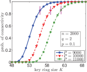
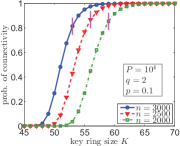
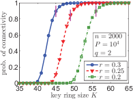
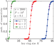
Figure 5: We plot the connectivity probability of the network $\mathbb{G}_{q}(n,\hskip 1.0ptK,\hskip 1.0ptP,\hskip 1.0ptr,\hskip 1.0pt\mathcal{T})$ with the $q$-composite scheme under transmission constraints, with respect to different key ring sizes $K$. Each vertical line presents the critical key ring size given by Eq. (13).

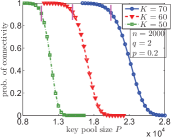
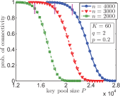
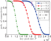
Figure 6: We plot the connectivity probability of the network $\mathbb{G}_{q}(n,\hskip 1.0ptK,\hskip 1.0ptP,\hskip 1.0ptr,\hskip 1.0pt\mathcal{T})$ with the $q$-composite scheme under transmission constraints, with respect to different key pool sizes $P$. Each vertical line presents the critical key pool size given by Eq. (14).

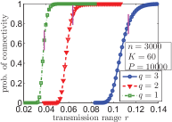
Figure 7: We plot the connectivity probability of the network $\mathbb{G}_{q}(n,\hskip 1.0ptK,\hskip 1.0ptP,\hskip 1.0ptr,\hskip 1.0pt\mathcal{T})$ with the $q$-composite scheme under transmission constraints, with respect to different transmission ranges $r$. Each vertical line presents the critical transmission range given by Eq. (15).

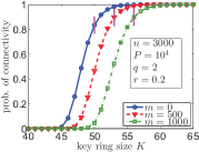
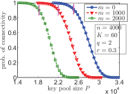
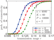
Figure 8: In the case where $m$ nodes have already been captured, we plot the connectivity probability of the network $\mathbb{G}_{q}(n,\hskip 1.0ptK,\hskip 1.0ptP,\hskip 1.0ptr,\hskip 1.0pt\mathcal{T})$ with the $q$-composite scheme under transmission constraints. Each vertical line in subfigures (a) (b) and (c) presents the critical key ring size given by Eq. (13), the critical key pool size given by Eq. (14), and the critical transmission range given by Eq. (15), respectively.

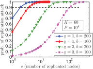
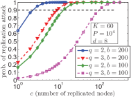
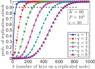
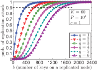
Figure 9: Plots for node replication attacks. We set the density of benign nodes as $d=1$ in subfigures (a) (c) and (d), while considering $d=8$ in subfigure (b).

IV Quantifying Node-Replication Attacks

IV-A Results

In secure sensor networks, a further attack following node capture is the so-called node-replication attack [24, 10, 38, 19]. The idea is that after node capture, the adversary can deploy replicas of compromised nodes by extracting keys from compromised nodes and then inserting some keys into the memory of replica nodes. The resources quantifying the adversary include the number of replicas deployed, and the cost of each replica. To characterize the cost of each replica, a simple metric is the number of keys inserted into its memory (of course, this may not be precise, but it provides qualitative intuition). The more a replica node cost, the more keys it can store. For a resource-limited adversary, it has to tradeoff between the number of replicas deployed, and the amount of keys kept on each replica. Unfortunately, prior studies on node-replication attacks lack of either formal or tractable analyses [24, 10, 38, 19] to determine the adversary’s optimal strategy. We closes this gap and present the following results:

• If $c$ denoting the number of replicas decreases by a factor of $\Delta$, then $b$ denoting the amount of keys on each replica should increase by a factor of $\sqrt[q]{\Delta}$ to achieve the same probability of a successful replication attack.

• If the adversary’s cost function $\textrm{cost}(b,c)$ scales with $b^{p_{b}}c^{p_{c}}$ for some $p_{b},p_{c}$, then the optimal $(b,c)$ to maximize the replication attack subject to the resource constraint $b^{p_{b}}c^{p_{c}}\leq\textrm{budget}$, depends on how the ratio $p_{b}/p_{c}$ compares with $q$. Specifically, the optimal $(b,c)$

  • is given by $b=\lfloor\sqrt[p_{b}]{\textrm{budget}}\rfloor$ and $c=1$ if $p_{b}/p_{c}<q$,

  • is given by $b=1$ and $c=\lfloor\sqrt[p_{c}]{\textrm{budget}}\rfloor$ if $p_{b}/p_{c}>q$, and

  • has many choices if $p_{b}/p_{c}=q$.

  In practice, when we often have $p_{b}/p_{c}<q$ (e.g., $p_{b}=1$, $p_{c}=1$ and $q>1$), then $b=\lfloor\sqrt[p_{b}]{\textrm{budget}}\rfloor$ and $c=1$ become optimal, meaning that the adversary should deploy a small number of high-cost sensors, rather than deploy a large number of low-cost sensors, to maximize the replication attack under a budget.

We now explain the above results (i) and (ii). Let the network density be $d$ (for benign nodes), so that the adversary can put a replica close to $d$ benign nodes on average. We compute the probability that a benign node shares at least $q$ keys with a replica (this will establish a secure link between them and thus induce a successful replication attack). Note that a benign node has $K_{n}$ keys selected from the pool of $P_{n}$ keys, and a replica has $d$ keys out of the same key pool. Then the probability that a benign node shares exactly $i$ keys with a replica is $\frac{\binom{b}{i}\binom{P_{n}-b}{K_{n}-i}}{\binom{P_{n}}{K_{n}}}$ (the idea is the benign node should have $i$ keys the same as the replica, and $K_{n}-i$ keys from the $(P_{n}-b)$-size key set in which the replica does not have a key. Then the probability that a replica and a benign node share at least (resp., less than) $q$ keys is $1-\alpha$ (resp., $\alpha$), where we denote $\sum\limits_{i=0}^{q-1}\frac{\binom{b}{i}\binom{P_{n}-b}{K_{n}-i}}{\binom{P_{n}}{K_{n}}}$ by $\alpha$ for simplicity. Since there are $c$ replicas deployed, and each replica is neighboring $d$ benign nodes on average, then the probability of a successful replication attack, defined as the probability that at least one replica and at least one benign node establish a secure link, can be computed as $1-\alpha^{cd}$. Similar to the result (35) on Page 35 for the link set-up probability $p_{s}$ in the $q$-composite scheme, an asymptotic result of $\alpha$ is $1-\frac{1}{q!}\cdot\frac{b^{q}{K_{n}}^{q}}{{P_{n}}^{q}}$, which we prove in the full version [34] due to space limitation (in fact, it is straightforward to see that $\alpha$ is $1-p_{s}$ if $b$ equals $K_{n}$). Hence, the probability of a successful replication attack (denoted by $p_{\textrm{replication}}$ below) asymptotically equals $1-(1-\frac{1}{q!}\cdot\frac{b^{q}{K_{n}}^{q}}{{P_{n}}^{q}})^{cd}$, which further becomes $\frac{cd}{q!}\cdot\frac{b^{q}{K_{n}}^{q}}{{P_{n}}^{q}}$ since the key pool size $P_{n}$ is much greater than $b$ and $K_{n}$. Then we see that $p_{\textrm{replication}}$ scales linearly with $c$, while scaling with $b^{q}$. This implies result (i); i.e., if $c$ denoting the number of replicas decreases by a factor of $\Delta$, then $b$ denoting the amount of keys on each replica should increase by a factor of $\sqrt[q]{\Delta}$ to achieve the same probability of a successful replication attack. We further obtain result (ii) by considering that the resource-constrained adversary maximizes $b^{q}c$ to maximize $p_{\textrm{replication}}$, subject to the resource constraint $b^{p_{b}}c^{p_{c}}\leq\textrm{budget}$.

IV-B Experiments

We present experiments in Figures 9 (a)–(d) on Page 9 to confirm the above results on replication attacks. In Figures 9 (a) and (b), we vary $c$ (the number of replicated nodes) given different $q$ and $b$ to plot $p_{\textrm{replication}}$. We consider node density $d=1$ in subfigure (a), and $d=8$ in subfigure (b). We also plot the horizontal line that corresponds to $p_{\textrm{replication}}$ being $0.9$. We take subfigure (a) as an example to validate our result (i) above. In Figure 9, after $c$ decreases by a factor of $\Delta$, then $b$ should increase by a factor of $\sqrt[q]{\Delta}$ to achieve the same $p_{\textrm{replication}}$. Let $c(b=100)$ and $c(b=200)$ denote $c$ corresponding to $b=100$ and $b=100$. Then for the upper two lines in Figure 9, given $q=1$, we compare ${\frac{c(b=100)}{c(b=200)}}$ with $2$, and the upper part of Table II shows they are actually equal for the data points presented. For the lower two lines in Figure 9, given $q=3$, we compare $\sqrt[3]{\frac{c(b=100)}{c(b=200)}}$ with $2$, and the lower part of Table II shows they are quite close for the data points presented. Hence, Table II has confirmed our results on replication attacks.

In Figures 9 (c) and (d), we vary $b$ (number of keys on each replica) given different $q$ to plot $p_{\textrm{replication}}$. We consider $c=10$ in subfigure (c), and $c=1$ in subfigure (d), and set node density $d=1$ in both subfigures. Recall that $p_{\textrm{replication}}$ scales with $\frac{cd}{q!}\big{(}\frac{bK_{n}}{P_{n}}\big{)}^{q}$, and thus decreases as $q$ increases for $bK_{n}$ smaller than $P_{n}$. This is confirmed in the plots.

TABLE II: This table confirms our results on replication attacks.

$q=1$ (the upper two lines in Figure 9)
prob	0.7	0.9	0.97	0.99
$c(b=100)$	2	4	6	8
$c(b=200)$	1	2	3	4
$\sqrt[q]{\frac{c(b=100)}{c(b=200)}}$	2	2	2	2
$q=3$ (the lower two lines in Figure 9)
prob	0.3	0.5	0.8	0.9
$c(b=100)$	17	43	75	104
$c(b=200)$	3	6	10	12
$\sqrt[q]{\frac{c(b=100)}{c(b=200)}}$	1.78	1.93	1.96	2.05

V Mathematical Details for
Resilience against Node Capture

We now provide formal details for our results in Section II on the resilience against node capture.

V-A Deriving $p_{\textnormal{compromised}}$

We consider the case where the adversary has captured some random set of $m$ nodes. As defined before, $p_{\textnormal{compromised}}$ is the probability that secure communication between two non-captured nodes is compromised by the adversary. With $\rho_{u}$ denoting the probability that two nodes share exactly $u$ keys in their key rings, for the $q$-composite scheme, Chan et al. [8] calculate $p_{\textnormal{compromised}}$ by

$$p_{\textnormal{compromised}} =\sum_{u=q}^{K_{n}}\bigg{\{}\bigg{[}1-\bigg{(}1-\frac{K_{n}}{P_{n}}\bigg{)}^{m}\bigg{]}^{u}\cdot\frac{\rho_{u}}{p_{s}}\bigg{\}}.$$ (19)

This result used in many studies [9, 23, 31, 29, 30] is unfortunately incorrect as formally shown by Yum and Lee [33]. With $A_{\tau}$ denoting the probability that the $m$ captured nodes have $\tau$ different keys in their key rings in total, where $K_{n}\leq\tau\leq\min\{mK_{n},P_{n}\}$, a correct computation [33] of $p_{\textnormal{compromised}}$ is as follows:

$$p_{\textnormal{compromised}}=\sum_{\tau=K_{n}}^{\min\{mK_{n},P_{n}\}}\Bigg{\{}A_{\tau}\cdot\sum_{u=q}^{K_{n}}\Bigg{[}\frac{\binom{\tau}{u}}{\binom{P_{n}}{u}}\cdot\frac{\rho_{u}}{p_{s}}\Bigg{]}\Bigg{\}},$$ (20)

where

$$A_{\tau} =\binom{P_{n}}{\tau}\cdot\frac{\binom{\tau}{K_{n}}^{m}-\sum_{\lambda=1}^{\tau-K_{n}}(-1)^{\lambda+1}\binom{\tau}{\lambda}\binom{\tau-\lambda}{K_{n}}^{m}}{\binom{P_{n}}{K_{n}}^{m}}.$$ (21)

Under a practical condition $P_{n}\geq 2K_{n}$, from the result [36, Proof of Lemma 2], it follows that

$$\frac{\rho_{u}}{p_{s}} =\frac{1}{u!}\frac{1}{[(K_{n}-u)!]^{2}}\frac{1}{(P_{n}-2K_{n}+u)!}$$

$$\quad\times\Bigg{\{}\sum_{u=q}^{K_{n}}\frac{1}{u!}\frac{1}{[(K_{n}-u)!]^{2}}\cdot\frac{1}{(P_{n}-2K_{n}+u)!}\Bigg{\}}^{-1}.$$ (22)

Substituting (21) and (22) into (20), we derive the exact formula of $p_{\textnormal{compromised}}$ through

$$p_{\textnormal{compromised}}$$

$$=\Bigg{\{}\sum_{u=q}^{K_{n}}\frac{1}{u!}\frac{1}{[(K_{n}-u)!]^{2}}\cdot\frac{1}{(P_{n}-2K_{n}+u)!}\Bigg{\}}^{-1}$$

$$~{}~{}\times\sum_{\tau=K_{n}}^{\min\{mK_{n},P_{n}\}}\Bigg{\{}\binom{P_{n}}{\tau}\sum_{u=q}^{K_{n}}\Bigg{[}\frac{\binom{\tau}{u}}{\binom{P_{n}}{u}}\cdot\frac{1}{u!}\frac{1}{[(K_{n}-u)!]^{2}}$$

$$\quad\times\frac{1}{(P_{n}-2K_{n}+u)!}\Bigg{]}\cdot\frac{\binom{\tau}{K_{n}}^{m}-\sum_{\lambda=1}^{\tau-K_{n}}(-1)^{\lambda+1}\binom{\tau}{\lambda}\binom{\tau-\lambda}{K_{n}}^{m}}{\binom{P_{n}}{K_{n}}^{m}}\Bigg{\}}.$$ (23)

We see that probability $p_{\textnormal{compromised}}$ relies on the parameters $K_{n},P_{n}$ and $q$, but does not directly depend on $n$. However, (23) is too complex to understand how $p_{\textnormal{compromised}}$ varies with respect to the parameters. To this end, we perform an asymptotic analysis in the remainder of this section to study $p_{\textnormal{compromised}}$; i.e., we analyze $p_{\textnormal{compromised}}$ as $n\to\infty$.

V-B Proof of Theorem 1

Recall that probability $p_{\textnormal{compromised}}$ is given by (20). From $P_{n}=\omega(mK_{n})$ which clearly follows from condition (1) (i.e., $m=o\big{(}\frac{P_{n}}{K_{n}}\big{)}$), it then holds (for all $n$ sufficiently large) that $\min\{mK_{n},P_{n}\}=mK_{n}$. Thus, we obtain from (20) that

$$p_{\textnormal{compromised}}=\sum_{\tau=K_{n}}^{mK_{n}}\Bigg{\{}A_{\tau}\cdot\sum_{u=q}^{K_{n}}\Bigg{[}\frac{\binom{\tau}{u}}{\binom{P_{n}}{u}}\cdot\frac{\rho_{u}}{p_{s}}\Bigg{]}\Bigg{\}}.$$ (24)

With $q\leq u\leq K_{n}$, we have

$$\binom{\tau}{u}\Bigg{/}\binom{P_{n}}{u}=\frac{\tau!}{u!(\tau-u)!}\bigg{/}\frac{P_{n}!}{u!(P_{n}-u)!}\leq\frac{\tau^{q}}{{(P_{n}-K_{n})}^{q}}.$$

Hence, from $\sum_{u=q}^{K_{n}}\rho_{u}=p_{s}$, it follows that

$$\sum_{u=q}^{K_{n}}\Bigg{[}\frac{\binom{\tau}{u}}{\binom{P_{n}}{u}}\cdot\frac{\rho_{u}}{p_{s}}\Bigg{]}\leq\sum_{u=q}^{K_{n}}\Bigg{[}\frac{\tau^{q}}{{(P_{n}-K_{n})}^{q}}\cdot\frac{\rho_{u}}{p_{s}}\Bigg{]}=\frac{\tau^{q}}{{(P_{n}-K_{n})}^{q}}.$$ (25)

Substituting (25) and $\sum_{\tau=K_{n}}^{mK_{n}}A_{\tau}=1$ into (24), we establish

$$p_{\textnormal{compromised}}\leq\sum_{\tau=K_{n}}^{mK_{n}}\Bigg{[}A_{\tau}\cdot\frac{\tau^{q}}{{(P_{n}-K_{n})}^{q}}\Bigg{]}\leq\frac{(mK_{n})^{q}}{{(P_{n}-K_{n})}^{q}}=o(1),$$ (26)

where the last step uses $mK_{n}=o(P_{n}-K_{n})$, which holds from condition $m=o\big{(}\frac{P_{n}}{K_{n}}\big{)}$.

V-C Proof of Corollary 1

Corollary 1 follows directly from Theorem 1 because $\frac{P_{n}}{K_{n}}=\Omega(n)$ and $m=o(n)$ together imply $m=o\big{(}\frac{P_{n}}{K_{n}}\big{)}$.

V-D Proof of Theorem 2

From the condition (3) (i.e., $m=o\big{(}\sqrt{\frac{P_{n}}{{K_{n}}^{2}}}\hskip 1.0pt\big{)}$), we find for $n$ sufficiently large that

$$m<\sqrt{\frac{P_{n}}{{K_{n}}^{2}}}=\frac{\sqrt{P_{n}}}{K_{n}}\leq\frac{P_{n}}{K_{n}},$$ (27)

so we further obtain $P_{n}>mK_{n}$ and hence $\min\{mK_{n},P_{n}\}=mK_{n}$. Then (24) still follows here.

As in (24), $p_{\textnormal{compromised}}$ is expressed as a summation of sequential elements with $\tau=K_{n},K_{n}+1,\ldots,mK_{n}$. Clearly, $p_{\textnormal{compromised}}$ is at least the element with $\tau=mK_{n}$; i.e.,

$$p_{\textnormal{compromised}} \geq A_{mK_{n}}\cdot\sum_{u=q}^{K_{n}}\Bigg{[}\frac{\binom{mK_{n}}{u}}{\binom{P_{n}}{u}}\cdot\frac{\rho_{u}}{p_{s}}\Bigg{]}.$$ (28)

The right hand side of (28) is also a summation. We only use its element with $u=q$. Then

$$p_{\textnormal{compromised}} \geq A_{mK_{n}}\cdot\frac{\binom{mK_{n}}{q}}{\binom{P_{n}}{q}}\cdot\frac{\rho_{q}}{p_{s}}.$$ (29)

The expression of $A_{mK_{n}}$ can be obtained from (21) by setting $\tau$ as $mK_{n}$, but it is very complex. We note that $A_{mK_{n}}$ has already been analyzed on Page II-B when we interpret (3). From our analysis therein, $A_{mK_{n}}$ equals $\frac{\prod_{j=0}^{m-1}\binom{P_{n}-jK_{n}}{K_{n}}}{\left[\binom{P_{n}}{K_{n}}\right]^{m}}$. Then it holds for all $n$ sufficiently large that

$$A_{mK_{n}} \geq\left[\frac{\binom{P_{n}-mK_{n}}{K_{n}}}{\binom{P_{n}}{K_{n}}}\right]^{m}\geq\left[\left(\frac{P_{n}-mK_{n}}{P_{n}}\right)^{K_{n}}\right]^{m}$$

$$=\left(1-\frac{mK_{n}}{P_{n}}\right)^{mK_{n}}\stackrel{{\scriptstyle(*)}}{{\geq}}1-\frac{(mK_{n})^{2}}{P_{n}},$$

where step (*) holds because

• $\frac{mK_{n}}{P_{n}}<1$ holds from (27) for all $n$ sufficiently large, and

• for $0\leq x<1$ and positive integer $y$, it holds that $(1-x)^{y}\geq 1-xy$; see our prior work [35, Page 20-Fact 2].

In view of condition (3) (i.e., $m=o\big{(}\sqrt{\frac{P_{n}}{{K_{n}}^{2}}}\hskip 1.0pt\big{)}$), we then have

$$A_{mK_{n}} \geq 1-o(1).$$ (30)

From condition (4), it follows that $mK_{n}=\omega(1)$. Since $q$ does not scale with $n$, then $mK_{n}=\omega(q)$. Therefore,

$$\binom{mK_{n}}{q}\Bigg{/}\binom{P_{n}}{q}=\frac{(mK_{n})!}{q!(mK_{n}-q)!}\bigg{/}\frac{P_{n}!}{q!(P_{n}-q)!}$$

$$\quad\geq\frac{(mK_{n}-q)^{q}}{{P_{n}}^{q}}=\frac{(mK_{n})^{q}}{{P_{n}}^{q}}\cdot[1-o(1)].$$ (31)

Clearly, (3) implies $\frac{{K_{n}}^{2}}{P_{n}}=o(1)$. Under (4) and $\frac{{K_{n}}^{2}}{P_{n}}=o(1)$, we use [36, Lemma 2] to derive

$${\rho_{q}}/{p_{s}} =1-o(1).$$ (32)

Applying (30) (31) and (32) to (29), we establish

$$p_{\textnormal{compromised}} \geq\frac{(mK_{n})^{q}}{{P_{n}}^{q}}\cdot[1-o(1)].$$ (33)

Since $\frac{{K_{n}}^{2}}{P_{n}}=o(1)$ implies $P_{n}=\omega(K_{n})$, we know from (26) that $p_{\textnormal{compromised}}$ is upper bounded by $\big{(}\frac{mK_{n}}{P_{n}}\big{)}^{q}\cdot[1+o(1)]$. This result and (33) together imply (5); i.e.,

$$p_{\textnormal{compromised}} \sim\bigg{(}\frac{mK_{n}}{P_{n}}\bigg{)}^{q}.$$ (34)

By [36, Lemma 2], under $\frac{{K_{n}}^{2}}{P_{n}}=o(1)$ and $K_{n}=\omega(1)$, it holds that

$$p_{s}\sim\frac{1}{q!}\bigg{(}\frac{{K_{n}}^{2}}{P_{n}}\bigg{)}^{q}.$$ (35)

Using (34) and (35), we obtain $\frac{p_{\textnormal{compromised}}}{p_{s}}\sim q!\big{(}\frac{m}{K_{n}}\big{)}^{q}.$ $\blacksquare$

V-E Proving Corollary 2

From Theorem 2, we have $\frac{p_{\textnormal{compromised}}}{p_{s}}\sim q!\big{(}\frac{m}{K_{n}}\big{)}^{q}$. Hence, to minimize $p_{\textnormal{compromised}}$ with respect to $q$ in the asymptotic sense given $p_{s}$, we will minimize $f(q)=q!\big{(}\frac{m}{K_{n}}\big{)}^{q}$. We derive $f(q+1)/f(q)$ as

$$\frac{f(q+1)}{f(q)} =\frac{m(q+1)}{K_{n}}.$$ (36)

Given (36), we obtain the following results.

• If $\frac{K_{n}}{m}<2$, as $q$ increases, the sequence $f(q)$ always increases, as it holds from (36) that
  for $q\geq 1$, then $\frac{f(q+1)}{f(q)}=\frac{m(q+1)}{K_{n}}\geq\frac{2m}{K_{n}}>1$.

• If $\frac{K_{n}}{m}=2$, then $f(1)=f(2)$. For $q\geq 2$, as $q$ increases, the sequence $f(q)$ increases, since we use (36) to derive that
  for $q\geq 2$, then $\frac{f(q+1)}{f(q)}=\frac{m(q+1)}{K_{n}}\geq\frac{3m}{K_{n}}=\frac{3}{2}.$

• If $\frac{K_{n}}{m}>2$, as $q$ increases, the sequence $f(q)$ first decreases, then increases, based on (36). In particular,

  • If $\frac{K_{n}}{m}$ is not an integer, then
    $f(1)>\ldots>f(\lfloor\frac{K_{n}}{m}\rfloor-1)>f(\lfloor\frac{K_{n}}{m}\rfloor)<f(\lfloor\frac{K_{n}}{m}\rfloor+1)<\ldots$, because we obtain from (36) that

    • $f(q+1)<f(q)$ for $q\leq\big{\lfloor}\frac{K_{n}}{m}\big{\rfloor}-1<\frac{K_{n}}{m}-1$, and

    • $f(q+1)>f(q)$ for $q\geq\big{\lfloor}\frac{K_{n}}{m}\big{\rfloor}>\frac{K_{n}}{m}-1$.

    Therefore, $f(q)$ achieves its minimum at $q=\big{\lfloor}\frac{K_{n}}{m}\big{\rfloor}$.

  • If $\frac{K_{n}}{m}$ is an integer, then
    $f(1)>\ldots>f(\frac{K_{n}}{m}-1)=f(\frac{K_{n}}{m})<f(\frac{K_{n}}{m}+1)<\ldots$, since we derive from (36) that

    • $f(q+1)<f(q)$ for $q<\frac{K_{n}}{m}-1$,

    • $f(q+1)=f(q)$ for $q=\frac{K_{n}}{m}-1$, and

    • $f(q+1)>f(q)$ for $q\geq\frac{K_{n}}{m}$.

    In this case, $f(q)$ achieves its minimum at both $q=\frac{K_{n}}{m}-1$ and $q=\frac{K_{n}}{m}$.

To summarize, an optimal $q$ to minimize $f(q)$ and hence minimize $p_{\textnormal{compromised}}$ is $q^{*}=\max\{\big{\lfloor}\frac{K_{n}}{m}\big{\rfloor},1\}$ (if $\frac{K_{n}}{m}$ is an integer greater than $1$, in addition to the above $q^{*}$, another optimal $q$ is $q=\frac{K_{n}}{m}-1$). $\blacksquare$

V-F Proving Corollary 3

From Theorem 2, we have $\frac{p_{\textnormal{compromised}}}{p_{s}}\sim q!\big{(}\frac{m}{K_{n}}\big{)}^{q}$, which implies $m\sim K_{n}\times(\frac{p_{\textnormal{compromised}}/p_{s}}{q!})^{1/q}$. Hence, to maximize $m$ with respect to $q$ in the asymptotic sense given $\frac{p_{\textnormal{compromised}}}{p_{s}}$ and $K_{n}$, the optimal $q$ is the solution to maximize $(\frac{p_{\textnormal{compromised}}/p_{s}}{q!})^{1/q}$. As noted in Corollary 3, the solution of $q$ is difficult to derive formally, but can given empirically by Table I and Figure 1.
   $\blacksquare$

VI Conclusion

The $q$-composite key predistribution scheme is of interest and significance as a mechanism to secure communications in wireless sensor networks. Our work evaluates the resilience of the $q$-composite scheme against node capture. We also derive the critical conditions to guarantee network connectivity with high probability despite node capture by the adversary, taking into account of practical transmission constraints. These results provide design guidelines for secure sensor networks using the $q$-composite scheme.

References

- [1] A. Alarifi and W. Du. Diversify sensor nodes to improve resilience against node compromise. In ACM Workshop on Security of Ad Hoc and Sensor Networks, pages 101–112, 2006.
- [2] S. R. Blackburn and S. Gerke. Connectivity of the uniform random intersection graph. Discrete Mathematics, 309(16), August 2009.
- [3] M. Bloznelis. Degree and clustering coefficient in sparse random intersection graphs. The Annals of Applied Probability, 23(3):1254–1289, 2013.
- [4] M. Bloznelis, J. Jaworski, and V. Kurauskas. Assortativity and clustering of sparse random intersection graphs. Electronic Journal of Probability, 18(38):1–24, 2013.
- [5] M. Bloznelis, J. Jaworski, and K. Rybarczyk. Component evolution in a secure wireless sensor network. Networks, 53:19–26, January 2009.
- [6] M. Bloznelis and T. Łuczak. Perfect matchings in random intersection graphs. Acta Mathematica Hungarica, 138(1-2):15–33, 2013.
- [7] T. Bonaci, L. Bushnell, and R. Poovendran. Node capture attacks in wireless sensor networks: A system theoretic approach. In Proc. IEEE Conference on Decision and Control (CDC), pages 6765–6772, 2010.
- [8] H. Chan, A. Perrig, and D. Song. Random key predistribution schemes for sensor networks. In Proc. IEEE Symposium on Security and Privacy, May 2003.
- [9] K. Chan and F. Fekri. A resiliency-connectivity metric in wireless sensor networks with key predistribution schemes and node compromise attacks. Physical Communication, 1(2):134 – 145, 2008.
- [10] M. Conti, R. Di Pietro, L. V. Mancini, and A. Mei. A randomized, efficient, and distributed protocol for the detection of node replication attacks in wireless sensor networks. In ACM International Symposium on Mobile Ad Hoc Networking and Computing, pages 80–89, 2007.
- [11] M. Conti, R. Di Pietro, L. V. Mancini, and A. Mei. Emergent properties: Detection of the node-capture attack in mobile wireless sensor networks. In Proc. ACM WiSec, pages 214–219, 2008.
- [12] R. Di Pietro, L. V. Mancini, A. Mei, A. Panconesi, and J. Radhakrishnan. Connectivity properties of secure wireless sensor networks. In ACM workshop on Security of Ad hoc and Sensor Networks, pages 53–58, 2004.
- [13] R. Di Pietro, L. V. Mancini, A. Mei, A. Panconesi, and J. Radhakrishnan. Sensor networks that are provably resilient. In Proc. Securecomm, pages 1–10, Aug 2006.
- [14] R. Di Pietro, L. V. Mancini, A. Mei, A. Panconesi, and J. Radhakrishnan. Redoubtable sensor networks. ACM Transactions on Information and Systems Security (TISSEC), 11(3):13:1–13:22, 2008.
- [15] W. Du, J. Deng, Y. S. Han, P. K. Varshney, J. Katz, and A. Khalili. A pairwise key predistribution scheme for wireless sensor networks. ACM Transactions on Information and System Security (TISSEC), 8(2):228–258, May 2005.
- [16] P. Erdős and A. Rényi. On random graphs, I. Publicationes Mathematicae (Debrecen), 6:290–297, 1959.
- [17] L. Eschenauer and V. Gligor. A key-management scheme for distributed sensor networks. In Proc. ACM CCS, 2002.
- [18] J. A. Fill, E. R. Scheinerman, and K. B. Singer-Cohen. Random intersection graphs when : An equivalence theorem relating the evolution of the and models. Random Structures & Algorithms, 16(2):156–176, Mar. 2000.
- [19] H. Fu, S. Kawamura, M. Zhang, and L. Zhang. Replication attack on random key pre-distribution schemes for wireless sensor networks. Computer Communications, 31(4):842–857, 2008.
- [20] P. Gupta and P. R. Kumar. Critical power for asymptotic connectivity in wireless networks. In Proc. IEEE CDC, pages 547–566, 1998.
- [21] B. Krishnan, A. Ganesh, and D. Manjunath. On connectivity thresholds in superposition of random key graphs on random geometric graphs. In Proc. IEEE International Symposium on Information Theory (ISIT), pages 2389–2393, 2013.
- [22] K. Krzywdziński and K. Rybarczyk. Geometric graphs with randomly deleted edges — connectivity and routing protocols. Mathematical Foundations of Computer Science, 6907:544–555, 2011.
- [23] D. Liu and P. Ning. Establishing pairwise keys in distributed sensor networks. In Proc. ACM CCS, pages 52–61, 2003.
- [24] B. Parno, A. Perrig, and V. Gligor. Distributed detection of node replication attacks in sensor networks. In IEEE Symposium on Security and Privacy (S&P’05), pages 49–63. IEEE, 2005.
- [25] M. Penrose. Random Geometric Graphs. Oxford University Press, July 2003.
- [26] M. D. Penrose et al. Connectivity of soft random geometric graphs. The Annals of Applied Probability, 26(2):986–1028, 2016.
- [27] K. Suzuki, D. Tonien, K. Kurosawa, and K. Toyota. Birthday paradox for multi-collisions. In International Conference on Information Security and Cryptology, pages 29–40. Springer, 2006.
- [28] P. Tague and R. Poovendran. Modeling node capture attacks in wireless sensor networks. In Annual Allerton Conference on Communication, Control, and Computing, pages 1221–1224, 2008.
- [29] T. M. Vu, R. Safavi-Naini, and C. Williamson. Securing wireless sensor networks against large-scale node capture attacks. In Proc. ACM ASIACCS, ASIACCS ’10, pages 112–123, 2010.
- [30] H. Yang, F. Ye, Y. Yuan, S. Lu, and W. Arbaugh. Toward resilient security in wireless sensor networks. In Proc. ACM MobiHoc, pages 34–45, 2005.
- [31] O. Yağan. Random Graph Modeling of Key Distribution Schemes in Wireless Sensor Networks. PhD thesis, Dept. of ECE, College Park (MD), June 2011. Available online at http://hdl.handle.net/1903/11910.
- [32] O. Yağan and A. M. Makowski. Random key graphs – can they be small worlds? In Proc. International Conference on Networks and Communications (NETCOM), pages 313 –318, December 2009.
- [33] D. H. Yum and P. J. Lee. Exact formulae for resilience in random key predistribution schemes. IEEE Transactions on Wireless Communications, 11(5):1638–1642, May 2012.
- [34] J. Zhao. On resilience and connectivity of secure wireless sensor networks under node capture attacks (full version). 2016. Available online at https://sites.google.com/site/workofzhao/TIFS-resilience.pdf
- [35] J. Zhao, O. Yağan, and V. Gligor. -connectivity in random key graphs with unreliable links. IEEE Transactions on Information Theory, 61(7):3810–3836, 2015.
- [36] J. Zhao. Topological properties of wireless sensor networks under the -composite key predistribution scheme with unreliable links. Technical Report CMU-CyLab-14-002, CyLab, Carnegie Mellon University, 2014.
- [37] J. Zhao, O. Yağan, and V. Gligor. Connectivity in secure wireless sensor networks under transmission constraints. In Allerton Conference on Communication, Control, and Computing, 2014.
- [38] B. Zhu, V. G. K. Addada, S. Setia, S. Jajodia, and S. Roy. Efficient distributed detection of node replication attacks in sensor networks. In Computer Security Applications Conference (ACSAC), pages 257–267, 2007.