Probabilistic Key Predistribution in Mobile Networks Resilient to Node-Capture Attacks

Abstract

We present a comprehensive analysis on connectivity and resilience of secure sensor networks under the widely studied $q$-composite key predistribution scheme. For network connectivity which ensures that any two sensors can find a path in between for secure communication, we derive the conditions to guarantee connectivity in consideration of (i) node-capture attacks, where the adversary may capture a set of sensors and compromise keys in their memory; (ii) sensor mobility, meaning that sensors can move around so that the network topology may change over time; (iii) physical transmission constraints, under which two sensors have to be within each other’s transmission range for communication; (iv) the boundary effect of network fields; and (v) link unreliability, meaning that links are allowed to be unreliable. In contrast, many prior connectivity analyses of secure sensor networks often ignore the above issues. For resilience, although limited studies have presented formal analysis, it is often assumed that the adversary captures a random set of sensors, whereas this paper allows the adversary to capture an arbitrary set of sensors. We present conditions to ensure unassailability and unsplittability in secure sensor networks under the $q$-composite scheme. Unassailability ensures that an adversary capturing any set consisting of a negligible fraction of sensors can compromise only a negligible fraction of communication links although the adversary may compromise communications between non-captured nodes which happen to use keys that are shared by captured nodes. Unsplittability means that when a negligible fraction of sensors are captured, almost all of the remaining nodes are still securely connected. Based on the results of connectivity, unassailability and unsplittability, we provide useful guidelines for the design of secure sensor networks.

I Introduction

I-A Background and Motivation

Random key predistribution schemes have been widely recognized as appropriate solutions to secure communications in resource-constrained wireless sensor networks [1, 2, 3, 4, 5, 6]. The idea of randomly assigning cryptographic keys to sensors before deployment was proposed in the seminal work of Eschenauer and Gligor [2]. The Eschenauer–Gligor (EG) scheme [2] works as follows. To secure a sensor network with $n$ nodes, in the key predistribution phase, the scheme uses a large key pool comprising $P_{n}$ cryptographic keys to select $K_{n}$ distinct keys uniformly at random for each sensor. These $K_{n}$ keys form the key ring of a sensor, and are inserted into the sensor’s memory. After sensors are deployed, two sensors can securely communicate over an existing link if and only if their key rings share at least one key. Common keys are found via neighbor discovery strategies [2]. We let ${P}_{n}$ and $K_{n}$ be functions of $n$ for generality, with the natural condition $1\leq K_{n}\leq P_{n}$.

Based on the EG scheme [2], Chan et al. [1] propose the $q$-composite key predistribution scheme as an extension. In such $q$-composite scheme, two sensors establish a secure link in between if and only if their key rings have at least $q$ key(s) in common, where $1\leq q\leq K_{n}$. Obviously, the $q$-composite scheme with $q=1$ is the same as the EG scheme. The $q$-composite scheme with $q\geq 2$ performs better than the EG scheme in terms of resilience against small-scale node-capture attacks while trading off heightened vulnerability in the presence of large-scale node-capture attacks. The $q$-composite scheme has been widely investigated in the literature over the last decade [7, 8, 9, 10, 11, 12, 13].

For wireless sensor networks with probabilistic key predistribution, due to the analytical complexity, most work in the literature on connectivity and resilience (explained below) considers only static networks with few exceptions. In this paper, we consider mobile networks in addition to static networks. An example application of probabilistic key predistribution to mobile networks beyond static sensor networks is frequency hopping [14], which is a classic approach for transmitting wireless signals by switching a carrier among different frequency channels. In this application, each node uniformly and independently selects $K_{n}$ secret seeds out of a secret pool consisting of $P_{n}$ secret seeds, and two nodes communicate with each other via frequency hopping only if they share at least certain number of secret seeds.

Although random key predistribution schemes enable secure communications in wireless sensor networks, they are often not explicitly designed to defend against node-capture attacks, which sensor networks deployed in hostile environments are often subject to. The resilience of random key predistribution schemes to node-capture attacks is often analyzed informally, and existing results are often obtained under full visibility without addressing physical transmission constraints, where the full visibility model assumes that any two sensors have a direct communication link in between. We present results on the resilience of the $q$-composite scheme not only under full visibility, but also under physical transmission constraints in which two nodes have to be within a certain distance from each other to communicate.

A metric proposed by Chan et al. [1] to address the resilience to node-capture attacks is the probability (denoted by $p_{\textnormal{compromised}}$) that capturing nodes enables an adversary to compromise communications between non-captured nodes. Such probability $p_{\textnormal{compromised}}$ is non-zero in the EG scheme and its $q$-composite version because non-captured nodes may happen to use keys that are also shared by captured nodes [15, 16]. Clearly, a random key predistribution scheme is perfectly resilient to sensor-capture attacks if $p_{\textnormal{compromised}}$ is alway zero. This implies that only communications between a captured node and its direct neighbors are compromised in a perfectly resilient scheme.

The EG scheme and its $q$-composite version can be easily extended to become perfectly resilient in the Chan et al. [1] sense [17, 18]. For instance, after the neighbor discovery phase of the EG scheme ends, in case that two neighboring nodes identified by $\textnormal{\emph{ID}}_{a}$ and $\textnormal{\emph{ID}}_{b}$ discover that they share key $k_{ab}$, they can each use a cryptographic hash function $hash(\cdot)$ to compute a new shared key $K_{ab}=hash(\textnormal{\emph{ID}}_{a}||\textnormal{\emph{ID}}_{b}||k_{ab})$ for $a<b$, and erase the old key $k_{ab}$. Since $K_{ab}$ is statistically unique up to the birthday bounds, the EG scheme becomes perfectly resilient. Similarly, the $q$-composite scheme can become perfectly resilient if the hash operation includes the uniquely ordered $q$ keys instead of the single key $k_{ab}$.

In mobile sensor networks employing the EG scheme or its $q$-composite version, the key hashing process above is not applicable, since sensors’ neighbor sets change over time as sensors move around. In static sensor networks with the key hashing process, there is still a neighbor discovery phase where perfect resilience cannot hold. Therefore, it is of interest and significance to analyze the resilience of $q$-composite scheme.

In addition to analyzing the resilience of the $q$-composite scheme, we also investigate connectivity properties of secure sensor networks under the $q$-composite scheme, when the adversary may capture a set of sensors. Connectivity means that any two sensors can find a path in between for secure communication. Our connectivity analysis considers many different settings: the network can be static or mobile; we consider the case of no node capture as well as the case of node-capture attacks; limited visibility models considered include the disk model, the link unreliability model, and their combination; under the disk model, we consider both the case ignoring the boundary effect of the network fields as well as the case considering the boundary effect.

I-B Problems

I-B1 Connectivity

Connectivity is a fundamental property that networks are often designed to have.

Definition of Connectivity. A network is connected if each node can find at least one path to reach another node.

For secure sensor networks with the $q$-composite scheme, we obtain the conditions to have the networks connected; i.e., the conditions that any two sensors can find a path in between for secure communication.

I-B2 Unsplittability

Another metric to characterize resiliency is unsplittability proposed by Pietro et al. [16]. The motivation is that even if a negligible (i.e., $o(1)$) fraction of nodes are compromised, almost all of the remaining nodes are still securely connected. Formally, unsplittability is defined as follows.

Definition of Unsplittability. A secure sensor network is unsplittable if with high probability an adversary that has captured an arbitrary set of $o(n)$ sensors cannot partition the network into two chunks, which both have linear sizes of sensors (i.e., $\Theta(n)$ sensors), and either are isolated from each other or only have compromised communications in between (i.e., keys used for communications between the two chucks are all compromised by the adversary).

From the definition above, for a unsplittable secure sensor network, even if $n_{1}=o(n)$ nodes are compromised, we still have a securely connected network consisting of $n-n_{2}$ nodes, where $n_{2}$ can also be written as $o(n)$ despite $n_{2}\geq n_{1}$. The reason for $n_{2}\geq n_{1}$ is that capturing nodes enables an adversary to compromise communications between non-captured nodes which happen to use keys that are also shared by captured nodes.

For secure sensor networks with the $q$-composite scheme, we explore the conditions to have the networks unsplittable.

I-B3 Unassailability

We borrow the notion of unassailability by Mei et al. [19] and present the following definition. Briefly, a secure sensor network is unassailable if $p_{\textnormal{compromised}}$ is $o(1)$ after the adversary has captured $o(n)$ sensors.

Definition of Unassailability. A secure sensor network is unassailable if an adversary that has captured an arbitrary set of $o(n)$ sensors can only compromise $o(1)$ fraction of communication links in the rest of the network; in other words, an adversary has to capture a constant fraction of sensors to compromise a constant fraction of communication links.

For secure sensor networks with the $q$-composite scheme, we derive the conditions to have the networks unassailable.

Many prior studies have analyzed node-captured attacks, but they often consider that the adversary randomly capture sensors. However, in practice, the adversary may tune its node-capture strategy according to its goals. To analyze unassailability, we analyze arbitrary node-capture attacks, in which the adversary can capture an arbitrary set of sensors. The choice of the captured nodes depends on the adversary’s goal and also physical limitations (e.g., some sensors may be easier to be captured than others).

Symbols	Meanings
$P_{n}$	the size of the key pool
$K_{n}$	the number of keys assigned to each sensor before deployment
$q$	the minimum number of keys that two sensors need to share for secure communication over an existing link
$r_{n}$	the distance that two sensors have to be within each other for communication under the disk model
$t_{n}$	the probability that each link is active when links are allowed to be unreliable

TABLE I: Symbols and their meanings.

I-C Contributions

Our work presents a rigorous and comprehensive analysis on resilience and connectivity of secure sensor networks under the $q$-composite key scheme. In particular, we investigate conditions to have unassailability and unsplittability. For network connectivity, we derive the conditions to guarantee connectivity in consideration of (i) node-capture attacks, where the adversary may capture a set of sensors and compromise keys in their memory; (ii) sensor mobility, meaning that sensors can move around so that the network topology may change over time; (iii) physical transmission constraints, under which two sensors have to be within each other’s transmission range for communication; (iv) the boundary effect of network fields; and (v) link unreliability, meaning that links are allowed to be unreliable.

Summary of Results. We summarize our results as follows. Note that all results are in the asymptotic sense.

• Connectivity: We establish the following results for connectivity in secure sensor networks employing the $q$-composite scheme. Note that $r_{n}$ denotes the distance that two sensors have to be within each other for communication under the disk model, and $t_{n}$ denotes the probability that each link is active when links are allowed to be unreliable.
  Connectivity of static networks:

  • A static secure sensor network with the $q$-composite scheme under the disk model on the unit torus without the boundary effect is connected if $\frac{1}{q!}\cdot\frac{{K_{n}}^{2q}}{{P_{n}}^{q}}\cdot\pi{r_{n}}^{2}\geq\frac{c\ln n}{n}$ for any constant $c>1$.

  • A static secure sensor network with the $q$-composite scheme and unreliable links under the disk model on the unit torus without the boundary effect is connected if $\frac{1}{q!}\cdot\frac{{K_{n}}^{2q}}{{P_{n}}^{q}}\cdot\pi{r_{n}}^{2}\cdot t_{n}\geq\frac{c\ln n}{n}$ for any constant $c>1$.

  • A static secure sensor network with the $q$-composite scheme under the disk model on the unit square with the boundary effect is connected if $\frac{1}{q!}\cdot\frac{{K_{n}}^{2q}}{{P_{n}}^{q}}\cdot\pi{r_{n}}^{2}$$\geq\frac{c\ln n}{n}$ for any constant $c>c_{n}^{*}:=\max$$\{1+\ln\frac{P_{n}}{{K_{n}}^{2}}\big{/}\ln n,$$~{}4\ln\frac{P_{n}}{{K_{n}}^{2}}\big{/}\ln n\}$.

  • A static secure sensor network with the $q$-composite scheme and unreliable links under the disk model on the unit square with the boundary effect is connected if $\frac{1}{q!}\cdot\frac{{K_{n}}^{2q}}{{P_{n}}^{q}}\cdot\pi{r_{n}}^{2}\cdot t_{n}\geq\frac{c\ln n}{n}$ for any constant $c>c_{n}^{\#}:=\max\{1+(q\ln\frac{P_{n}}{{K_{n}}^{2}}+\ln\frac{1}{t_{n}})\big{/}\ln n,~{}4(q\ln\frac{P_{n}}{{K_{n}}^{2}}+\ln\frac{1}{t_{n}})\big{/}\ln n\}$.

  Connectivity of mobile networks:

  • A mobile secure sensor network with the $q$-composite scheme under the disk model on the unit torus without the boundary effect and under the i.i.d. mobility model is connected for at least $n^{c-1-\epsilon}$ consecutive time slots from the beginning for an arbitrary positive constant $\epsilon$, if $\frac{1}{q!}\cdot\frac{{K_{n}}^{2q}}{{P_{n}}^{q}}\cdot\pi{r_{n}}^{2}\geq\frac{c\ln n}{n}$ for any constant $c>1$.

  • A mobile secure sensor network with the $q$-composite scheme and unreliable links under the disk model on the unit torus without the boundary effect and under the i.i.d. mobility model is connected for at least $n^{c-1-\epsilon}$ consecutive time slots from the beginning for an arbitrary positive constant $\epsilon$, if $\frac{1}{q!}\cdot\frac{{K_{n}}^{2q}}{{P_{n}}^{q}}\cdot\pi{r_{n}}^{2}\cdot t_{n}\geq\frac{c\ln n}{n}$ for any constant $c>1$.

  • A mobile secure sensor network with the $q$-composite scheme under the disk model on the unit square with the boundary effect and under the i.i.d. mobility model is connected for at least $n^{c-c_{n}^{*}-\epsilon}$ consecutive time slots from the beginning for an arbitrary positive constant $\epsilon$, if $\frac{1}{q!}\cdot\frac{{K_{n}}^{2q}}{{P_{n}}^{q}}\cdot\pi{r_{n}}^{2}\geq\frac{c\ln n}{n}$ for any constant $c>c_{n}^{*}$ with $c_{n}^{*}$ defined above.

  • A mobile secure sensor network with the $q$-composite scheme and unreliable links under the disk model on the unit square with the boundary effect and under the i.i.d. mobility model is connected for at least $n^{c-c_{\#}-\epsilon}$ consecutive time slots from the beginning for an arbitrary positive constant $\epsilon$, if $\frac{1}{q!}\cdot\frac{{K_{n}}^{2q}}{{P_{n}}^{q}}\cdot\pi{r_{n}}^{2}\cdot t_{n}\geq\frac{c\ln n}{n}$ for any constant $c>c_{n}^{\#}$ with $c_{n}^{\#}$ defined above.

  Connectivity under node capture: To obtain the connectivity results for an $n$-size network after the adversary has captured a random set of $m$ nodes out of all $n$ nodes, we just replace $\ln n$ with $\ln(n-m)$, $\frac{\ln n}{n}$ with $\frac{\ln(n-m)}{n-m}$, and $n$ with $(n-m)$ in the above connectivity results (note that we do not replace the “$n$” in $K_{n}$, $P_{n}$, $r_{n}$, $t_{n}$).

• Unassailability:

  • A secure sensor network with the $q$-composite scheme under any communication model is unassailable if ${P_{n}}/{K_{n}}=\Omega(n)$.

• Unsplittability:

  • A secure sensor network with the $q$-composite scheme under full visibility is unsplittable if $\frac{1}{q!}\cdot\frac{{K_{n}}^{2q}}{{P_{n}}^{q}}\geq\frac{c\ln n}{n}$ for any constant $c>1$, $K_{n}=\omega(\ln n)$ and $K_{n}=o\big{(}\min\{\sqrt{P_{n}},\frac{P_{n}}{n}\}\big{)}$.

  • A static secure sensor network with the $q$-composite scheme under the disk model on some area $\mathcal{A}$ is splittable if $r_{n}=o(\sqrt{\mathcal{A}})$.

I-D Roadmap

The rest of the paper is organized as follows. Section II reviews related work. In Section III, we describe the system model. Section IV presents the main results. We provide several useful lemmas in Section V. Afterwards, we establish the theorems in Section VI. We explain simulation results in Section VII. Finally, Section VIII concludes the paper.

II Related Work

Unassailability. Mei et al. [19] introduce the notion of unassailability. However, their work is different from ours in the following aspects: they address the EG scheme whereas we consider the more general $q$-composite scheme; they assume that the adversary knows the key rings of all nodes whereas we do not have such assumption; they enforce the strong assumption that whenever the adversary has compromised one shared key between two sensors, the secure link between the two sensors is compromised even though that compromised key is not used for the secure link. For the EG scheme, Di Pietro et al. [15, 16] have presented conditions to ensure that an adversary has to capture a constant fraction of sensors in order to compromise a constant fraction of communication links. Similar results for the $q$-composite scheme have been obtained by Zhao [17, 18]. However, the difference between [15, 16, 17, 18] and this paper is that [15, 16, 17, 18] consider an adversary randomly capturing sensors, while this paper investigates the more practical case of arbitrary node-capture attacks, in which the adversary can capture an arbitrary set of sensors. In addition to the EG scheme and the $q$-composite scheme, the random pairwise key predistribution scheme of Chan et al. [1] has also received much attention. The unassailability of the pairwise scheme has recently been studied by Yağan and Makowski [20]. The key predistribution schemes by Liu and Ning [12] and Du et al. [3] exhibit the threshold behavior in terms of resilience against node-capture attacks. Techniques to improve the resilience against node capture have been studied in [21, 22, 23, 24, 25, 26].

Unsplittability. For the EG scheme, its unsplittability has been studied by [16]. Note that our unsplittability result is for the more general $q$-composite scheme. Yet, even when we apply our general result to the EG scheme, the obtained result will be stronger than that of [16]. Specifically, since our unsplittability condition for the $q$-composite scheme uses $\frac{1}{q!}\cdot\frac{{K_{n}}^{2q}}{{P_{n}}^{q}}\geq\frac{c\ln n}{n}$ for a constant $c>1$, our unsplittability result applying to the EG scheme (i.e., the $q$-composite scheme with $q=1$) uses $\frac{{K_{n}}^{2}}{{P_{n}}}\geq\frac{c\ln n}{n}$ for a constant $c>1$. In contrast, the unsplittability result of the EG scheme in [16] requires $\frac{{K_{n}}^{2}}{{P_{n}}}\geq\frac{c\ln n}{n}$ for a constant $c>17$. For the random pairwise key predistribution scheme of Chan et al. [1], Yağan and Makowski [20] have recently studied its unsplittability.

Connectivity. Although connectivity of secure sensor networks has been widely investigated in the literature, many prior studies has one or more than one of the following limitations: much research [6, 4, 1] ignores either real-world transmission constraints between sensors or mobility of sensors because analyzing the key predistribution scheme, transmission constraints, and node mobility together makes the analysis very challenging; several researches considering transmission constraints obtain quite weak results [27, 28, 29, 10] or apply to limited settings [17] (e.g., the case ignoring the boundary effect of the network fields); the proof techniques [30] lack formality. Below we discuss some related work in detail.

For a secure sensor network with the $q$-composite scheme under the full visibility, its connectivity has been studied in [30, 10], while its $k$-connectivity has been considered in [29], where $k$-connectivity ensures connectivity despite the failure of any $k-1$ nodes [31, 32]. However, the proof techniques in [30] lack formality (specifically [30, Equation (6.93)]) and are different from those in this paper. The results of connectivity in [29] and $k$-connectivity in [10] address only the narrow and impractical range of $P_{n}=o\big{(}n^{\frac{1}{q}}(\ln n)^{-\frac{3}{5q}}\big{)}$, as explained below. In contrast, from condition set $\Lambda$ in (6), our Theorem 1 considers a more practical range of $P_{n}=\omega(n\ln n)$. We present more details below.

We explain that the result of [10] for connectivity is not applicable to practical sensor networks, whereas our result is applicable. The limitation of [10] is that both $K_{n}$ and $P_{n}$ are required to be quite small in [10] so they will not satisfy the resiliency requirement $\frac{P_{n}}{K_{n}}=\Omega(n)$. More specifically, [10, Equation (2)] enforces

$$\left[(q+2)\binom{K_{n}}{q}^{5}(\ln\ln n)^{2}\right]^{\frac{3K_{n}-q}{3(K_{n}-q)}} \leq(\ln n)^{1-\gamma}$$

$$\text{for a constant }\gamma\in(0,1),$$ (1)

where the notation $s$ and $d$ in [10] correspond to $q$ and $K_{n}$ here.

In (1), the exponent $\frac{3K_{n}-q}{3(K_{n}-q)}$ is greater than $1$ given $K_{n}>q$, since $q$ is a constant and does not scale with $n$ ($q$ is often less than $10$), while $K_{n}$ controls the number of keys on each sensor and is at least a two-digit number for a network comprising thousands of sensors. In fact, if $K_{n}<q$, the $q$-composite scheme is meaningless because each sensor has just $K_{n}$ keys so it is impossible for two sensors to share $q$ keys if $K_{n}<q$. Furthermore, in (1), the base is greater than $1$ for all sufficiently large owing to $\lim_{n\to\infty}\ln\ln n=\infty$. Given the above, we can cancel out the exponent in (1); i.e., (1) implies

$$(q+2)\binom{K_{n}}{q}^{5}(\ln\ln n)^{2}\leq(\ln n)^{1-\gamma}$$

$$\text{for a constant }\gamma\in(0,1).$$ (2)

In view of $\binom{K_{n}}{q}=\frac{1}{q!}\prod_{i=0}^{q-1}(K_{n}-i)\geq\frac{1}{q!}(K_{n}-q)^{q}$, we use (2) to derive

$$K_{n}\leq q+\sqrt[q]{q!}\cdot\sqrt[5q]{\frac{1}{q+2}\cdot\frac{(\ln n)^{1-\gamma}}{(\ln\ln n)^{2}}}$$

$$\text{for a constant }\gamma\in(0,1),$$ (3)

which along with the fact that $q$ is a constant further induces

$$K_{n} =O\left(\sqrt[5q]{\frac{(\ln n)^{1-\gamma}}{(\ln\ln n)^{2}}}\right)=o\left((\ln n)^{\frac{1}{5q}}\right).$$ (4)

To ensure connectivity of a secure sensor network resulted from the $q$-composite key predistribution scheme, with $p_{q}$ denoting the edge probability, both [10] and our work obtain that it is necessary to have $p_{q}=\Omega\big{(}\frac{\ln n}{n}\big{)}$ or equivalently $\frac{1}{q!}\cdot\frac{{K_{n}}^{2q}}{{P_{n}}^{q}}=\Omega\big{(}\frac{\ln n}{n}\big{)}$, since it holds that $\frac{1}{q!}\cdot\frac{{K_{n}}^{2q}}{{P_{n}}^{q}}$ is an asymptotic expression of $p_{q}$ from (18) later. The requirement $\frac{1}{q!}\cdot\frac{{K_{n}}^{2q}}{{P_{n}}^{q}}=\Omega\big{(}\frac{\ln n}{n}\big{)}$ and the condition (4) derived from [10] together imply

$$P_{n} =\frac{{K_{n}}^{2}}{\sqrt[q]{q!\times\Omega\big{(}\frac{\ln n}{n}\big{)}}}=o\left(n^{\frac{1}{q}}(\ln n)^{-\frac{3}{5q}}\right).$$ (5)

However, we explain that (5) is not applicable to practical sensor networks. This paper for general $q$ and Di Pietro et al. [15, 16] for $q=1$ have both proved that the condition $\frac{P_{n}}{K_{n}}=\Omega(n)$ is needed to ensure reasonable network resiliency against node-capture attacks in the sense that an adversary capturing sensors at random has to obtain at least a constant fraction of nodes of the network in order to compromise a constant fraction of secure links. The condition $\frac{P_{n}}{K_{n}}=\Omega(n)$ with $K_{n}\geq 1$ clearly implies $P_{n}=\Omega(n)$, which does not hold for any $P_{n}$ satisfying (5). Hence, we have explained that the result of [10] cannot be used to design secure sensor networks in practice. In contrast, from condition set $\Lambda$ in (6), our theorems apply to a more practical range of $P_{n}=\omega(n\ln n)$. Hence, our results apply to real-world secure sensor networks and provide useful design guidelines.

For connectivity analysis of secure sensor networks taking into transmission constraints, for the EG scheme, Krzywdziński and Rybarczyk [28], and Krishnan et al. [27] recently show upper bounds $\frac{8\ln n}{n}$ and $\frac{2\pi\ln n}{n}$ for the critical threshold that the edge probability (i.e., the probability of a secure link between two sensors) takes for connectivity, while [14] proves the exact threshold as $\frac{\ln n}{n}$. For the $q$-composite scheme with general $q$, [17] has presented connectivity results under transmission constraints. However, the following issues addressed in this paper are not tackled by [17]: the boundary effect of the network fields, the mobility of sensors, the combination of link unreliability and the transmission constraints modeled by the disk model (to be explained in Section III-A2). We note that there are many connectivity studies [5, 4, 33, 34, 35, 36] considering only link unreliability without the disk model (node mobility and node-capture attacks are not considered in these references).

III System Models

All of our studied networks employ the $q$-composite scheme. Clearly, our analysis also applies to the basic Eschenauer–Gligor scheme which has $q=1$. We first discuss the communication models and mobility, and then detail the studied networks.

III-A Communication Models

We consider the following communication models.

III-A1 Full Visibility

The full visibility model assumes that any two sensors have a direct communication link in between. Under such model, a secure link exists between two sensors if and only if they share at least $q$ keys.

III-A2 Disk Model

In the disk model, each node’s transmission area is a disk with a transmission radius $r_{n}$, with $r_{n}$ being a function of $n$ for generality. Two nodes have to be within $r_{n}$ (their distance is at most $r_{n}$) for direct communication. As for the node distribution, the same as much previous work [27, 28, 37, 38], we consider that the $n$ nodes are independently and uniformly deployed in some network region $\mathcal{A}$. We let the region $\mathcal{A}$ be either a torus $\mathcal{T}$ or a square $\mathcal{S}$, each with a unit area. The unit torus $\mathcal{T}$ eliminates the boundary effect (a node on $\mathcal{T}$ “exits” the area from one side appears as reentering from the opposite side). The boundary effect of the unit square $\mathcal{S}$ is that a circle with radius $r_{n}$ centered a point near the boundary of $\mathcal{S}$ may have a part falling outside of $\mathcal{S}$, so a node close to one side and another node close to the opposite side may not have an edge in between on the square $\mathcal{S}$, but may have an edge in between on the torus $\mathcal{T}$ because of wrap-around connections of torus topology.

III-A3 Link Unreliability

Communication links between nodes may not be available due to the presence of physical barriers between nodes or because of harsh environmental conditions severely impairing transmission. To model unreliable links, each link is either active with probability $t_{n}$ or inactive with probability $(1-t_{n})$, where $t_{n}$ is a function of $n$ for generality.

Table I summarizes the symbols and their meanings.

III-B Mobility

In addition to static sensor networks, we also consider mobile sensor networks which are initialized in the same way as static sensor networks. After initialization, sensors may move around. On either the torus or the square, we consider the i.i.d. mobility model, where each node independently picks a new location uniformly at random at the beginning of a time slot and stays at the location in the rest of the time slot. This i.i.d. mobility model clearly yields a uniform node distribution at each time slot. For each mobile network that we consider, given a uniform node distribution at each time slot, we can view the mobile network at a single time slot as an instance of the corresponding static network. A future work is to consider other mobility models [39, 40, 41, 42].

III-C Studied Networks

We summarize our studied networks in Table II. As presented, we consider the following nine secure sensor networks:

• a secure sensor network with the $q$-composite scheme under full visibility (the network can be either static or mobile),

• a static secure sensor network with the $q$-composite scheme under the disk model on the unit torus without the boundary effect,

• a static secure sensor network with the $q$-composite scheme under the disk model on the unit square with the boundary effect,

• a static secure sensor network with the $q$-composite scheme and unreliable links under the disk model on the unit torus without the boundary effect,

• a static secure sensor network with the $q$-composite scheme and unreliable links under the disk model on the unit square with the boundary effect,

• a mobile secure sensor network with the $q$-composite scheme under the disk model on the unit torus without the boundary effect,

• a mobile secure sensor network with the $q$-composite scheme under the disk model on the unit square with the boundary effect,

• a mobile secure sensor network with the $q$-composite scheme and unreliable links under the disk model on the unit torus without the boundary effect, and

• a mobile secure sensor network with the $q$-composite scheme and unreliable links under the disk model on the unit square with the boundary effect.

Settings			Notation for networks
full visibility (static/mobile secure sensor networks)			$\textnormal{network}^{\textnormal{full visibility}}$
static secure sensor networks	disk model	torus	$\textnormal{static-network}^{\textnormal{disk model}}_{\textnormal{unit torus}}$
		square	$\textnormal{static-network}^{\textnormal{disk model}}_{\textnormal{unit square}}$
	disk model w/ unreliable links	torus	$\textnormal{static-network}^{\begin{subarray}{\textnormal{missing}}{\textnormal{disk model}}\\ \textnormal{unit torus}\end{subarray}}_{\textnormal{unreliable links}}$
		square	$\textnormal{static-network}^{\begin{subarray}{\textnormal{missing}}{\textnormal{disk model}}\\ \textnormal{unit square}\end{subarray}}_{\textnormal{unreliable links}}$
mobile secure sensor networks	disk model	torus	$\textnormal{mobile-network}^{\textnormal{disk model}}_{\textnormal{unit torus}}$
		square	$\textnormal{mobile-network}^{\textnormal{disk model}}_{\textnormal{unit square}}$
	disk model w/ unreliable links	torus	$\textnormal{mobile-network}^{\begin{subarray}{\textnormal{missing}}{\textnormal{disk model}}\\ \textnormal{unit torus}\end{subarray}}_{\textnormal{unreliable links}}$
		square	$\textnormal{mobile-network}^{\begin{subarray}{\textnormal{missing}}{\textnormal{disk model}}\\ \textnormal{unit square}\end{subarray}}_{\textnormal{unreliable links}}$

TABLE II: The studied secure sensor networks and their notation, where “w/” is short for “with”. All networks employ the $q$-composite random key predistribution scheme.

Throughout the paper, $q$ is an arbitrary positive integer and does not scale with $n$, the number of nodes in the sensor network. In addition, $\ln$ is the natural logarithm function, the base of which is $e$.

IV Main Results

We present the main results below.

IV-A Connectivity of Secure Sensor Networks

We establish connectivity results for the nine settings of secure sensor networks in Table II. A network is connected if each node can find at least one path to securely communicate with another node. The results are summarized in Table III, and they will be presented as theorems in detail.

Settings			Connectivity results
static/mobile secure sensor networks under full visibility			connected if $\frac{1}{q!}\cdot\frac{{K_{n}}^{2q}}{{P_{n}}^{q}}\geq\frac{c\ln n}{n}$ for any constant $c>1$
static secure sensor networks	disk model	torus	connected if $\frac{1}{q!}\cdot\frac{{K_{n}}^{2q}}{{P_{n}}^{q}}\cdot\pi{r_{n}}^{2}\geq\frac{c\ln n}{n}$ for any constant $c>1$
		square	connected if $\frac{1}{q!}\cdot\frac{{K_{n}}^{2q}}{{P_{n}}^{q}}\cdot\pi{r_{n}}^{2}\geq\frac{c\ln n}{n}$ for any constant $c>c_{n}^{*}$
	disk model w/ unreliable links	torus	connected if $\frac{1}{q!}\cdot\frac{{K_{n}}^{2q}}{{P_{n}}^{q}}\cdot\pi{r_{n}}^{2}\cdot t_{n}\geq\frac{c\ln n}{n}$ for any constant $c>1$
		square	connected if $\frac{1}{q!}\cdot\frac{{K_{n}}^{2q}}{{P_{n}}^{q}}\cdot\pi{r_{n}}^{2}\cdot t_{n}\geq\frac{c\ln n}{n}$ for any constant $c>c_{n}^{\#}$
mobile secure sensor networks	disk model	torus	connected for at least $n^{c-1-\epsilon}$ consecutive time slots if $\frac{1}{q!}\cdot\frac{{K_{n}}^{2q}}{{P_{n}}^{q}}\cdot\pi{r_{n}}^{2}\geq\frac{c\ln n}{n}$ for any constant $c>1$
		square	connected for at least $n^{c-c_{n}^{*}-\epsilon}$ consecutive time slots if $\frac{1}{q!}\cdot\frac{{K_{n}}^{2q}}{{P_{n}}^{q}}\cdot\pi{r_{n}}^{2}\geq\frac{c\ln n}{n}$ for any constant $c>c_{n}^{*}$
	disk model w/ unreliable links	torus	connected for at least $n^{c-1-\epsilon}$ consecutive time slots if $\frac{1}{q!}\cdot\frac{{K_{n}}^{2q}}{{P_{n}}^{q}}\cdot\pi{r_{n}}^{2}\cdot t_{n}\geq\frac{c\ln n}{n}$ for any constant $c>1$
		square	connected for at least $n^{c-c_{n}^{\#}-\epsilon}$ consecutive time slots if $\frac{1}{q!}\cdot\frac{{K_{n}}^{2q}}{{P_{n}}^{q}}\cdot\pi{r_{n}}^{2}\cdot t_{n}\geq\frac{c\ln n}{n}$ for any constant $c>c_{n}^{\#}$

TABLE III: Different settings of secure sensor networks and their connectivity results, where “w/” is short for “with”. Note that $c_{n}^{*}$ is $\max\Big{\{}1+\big{(}\ln\frac{P_{n}}{{K_{n}}^{2}}\big{)}\big{/}\ln n,~{}4\big{(}\ln\frac{P_{n}}{{K_{n}}^{2}}\big{)}\big{/}\ln n\Big{\}}$, $c_{n}^{\#}$ is $c_{n}^{\#}$ is $\max\Big{\{}1+\big{(}q\ln\frac{P_{n}}{{K_{n}}^{2}}+\ln\frac{1}{t_{n}}\big{)}\big{/}\ln n,~{}4\big{(}q\ln\frac{P_{n}}{{K_{n}}^{2}}+\ln\frac{1}{t_{n}}\big{)}\big{/}\ln n\Big{\}}$, and $\epsilon$ is an arbitrary positive constant. All results are in the asymptotic sense to hold with high probability, and thus the conditions in the table only need to hold for all $n$ sufficiently large. Except the result under full visibility which requires conditions on $K_{n}$ and $P_{n}$ in condition set $\Lambda$ in (6) on Page 6 but not the condition $r_{n}=o(1)$ in $\Lambda$, all other results need the whole condition set $\Lambda$.

All results given in Table III rely a set $\Lambda$ of conditions, defined as follows:

$$\textnormal{Condition set }\Lambda:\begin{cases}K_{n}&=\omega(\ln n),\\ K_{n}\hskip 1.0pt&=o\Big{(}\min\big{\{}\sqrt{P_{n}},\frac{P_{n}}{n}\big{\}}\Big{)},\\ \hskip 2.0ptr_{n}&=o(1).\end{cases}$$ (6)

We explain that all conditions in set $\Lambda$ are practical. Note that $K_{n}$ is the number of keys assigned to each sensor before deployment. In real-world implementations, $K_{n}$ is often larger [4, 8] than $\ln n$, so $K_{n}=\omega(\ln n)$ follows. As concrete examples, we have $\ln 1000\approx 6.9$, $\ln 5000\approx 8.5$ and $\ln 10000\approx 9.2$. Since $K_{n}$ is much smaller compared to both $n$ and $P_{n}$ due to constrained memory and computational resources of sensors [2, 1, 4], then $\frac{{K_{n}}^{2}}{P_{n}}=o(1)$ and $\frac{K_{n}}{P_{n}}=o\big{(}\frac{1}{n}\big{)}$ are practical, yielding $K_{n}=o\big{(}\min\{\sqrt{P_{n}},\frac{P_{n}}{n}\}\big{)}$. Note that $K_{n}=\omega(\ln n)$ and $K_{n}=o\big{(}\min\{\sqrt{P_{n}},\frac{P_{n}}{n}\}\big{)}$ together imply $P_{n}=\omega(n\ln n)$, which is also practical since $P_{n}$ is larger than $n$ [2, 1, 16]. As examples, we have $1000\ln 1000\approx 6907$, $5000\ln 5000\approx 42585$ and $10000\ln 10000\approx 92103$. Finally, because we consider a unit area of network region and there are $n$ nodes in this region, the condition $r_{n}=o(1)$ is also practical.

To look at the conditions related to $\frac{\ln n}{n}$ in Table III, we first explain that for each network in Table III, the left hand side of each condition related to $\frac{\ln n}{n}$ in the result is asymptotically equivalent to the edge probability of the network, where the edge probability is the probability that two nodes have an edge in between for direct communication, and is defined for each time slot for mobile networks (note that all nodes are symmetric in each network). Specifically, we have the following under condition set $\Lambda$:

• $\frac{1}{q!}\cdot\frac{{K_{n}}^{2q}}{{P_{n}}^{q}}$ is asymptotically equivalent to the edge probability of $\textnormal{network}^{\textnormal{full visibility}}$,

• $\frac{1}{q!}\cdot\frac{{K_{n}}^{2q}}{{P_{n}}^{q}}\cdot\pi{r_{n}}^{2}$ is a common asymptotic value of the edge probabilities of networks $\textnormal{static-network}^{\textnormal{disk model}}_{\textnormal{unit torus}}$, $\textnormal{static-network}^{\textnormal{disk model}}_{\textnormal{unit square}}$, $\textnormal{mobile-network}^{\textnormal{disk model}}_{\textnormal{unit torus}}$, and $\textnormal{mobile-network}^{\textnormal{disk model}}_{\textnormal{unit square}}$, and

• $\frac{1}{q!}\cdot\frac{{K_{n}}^{2q}}{{P_{n}}^{q}}\cdot\pi{r_{n}}^{2}\cdot t_{n}$ is a common asymptotic value of the edge probabilities of $\textnormal{static-network}^{\begin{subarray}{\textnormal{missing}}{\textnormal{disk model}}\\ \textnormal{unit torus}\end{subarray}}_{\textnormal{unreliable links}}$, $\textnormal{static-network}^{\begin{subarray}{\textnormal{missing}}{\textnormal{disk model}}\\ \textnormal{unit square}\end{subarray}}_{\textnormal{unreliable links}}$, $\textnormal{mobile-network}^{\begin{subarray}{\textnormal{missing}}{\textnormal{disk model}}\\ \textnormal{unit torus}\end{subarray}}_{\textnormal{unreliable links}}$, and $\textnormal{mobile-network}^{\begin{subarray}{\textnormal{missing}}{\textnormal{disk model}}\\ \textnormal{unit square}\end{subarray}}_{\textnormal{unreliable links}}$.

Before explaining the above results ①–③, we first present a useful result (i.e., Lemma 1) and its proof.

Lemma 1.

Let $\mu_{n}(\mathcal{A})$ be the probability that two nodes are within distance $r_{n}$ when they are independently and uniformly distributed in a network region $\mathcal{A}$. Then we have:

• When $\mathcal{A}$ is a torus $\mathcal{T}$ of unit area, $\mu_{n}(\mathcal{A})$ becomes $\mu_{n}(\mathcal{T})$, which is given by

  $$\textstyle{\mu_{n}(\mathcal{T})=\pi{r_{n}}^{2},\text{ for }r_{n}\leq\frac{1}{2}}.$$ (7)

• When $\mathcal{A}$ is a square $\mathcal{S}$ of unit area, $\mu_{n}(\mathcal{A})$ becomes $\mu_{n}(\mathcal{S})$, which satisfies

  $$\textstyle{(1-2{r_{n}})^{2}\cdot\pi{r_{n}}^{2}\leq\mu_{n}(\mathcal{S})\leq\pi{r_{n}}^{2},\text{ for }r_{n}\leq\frac{1}{2}},$$ (8)

  and

  $$\textstyle{\mu_{n}(\mathcal{S})\sim\pi{r_{n}}^{2},\text{ for }r_{n}=o(1)},$$ (9)

where $\mu_{n}(\mathcal{S})\sim\pi{r_{n}}^{2}$ means $\lim_{n\to\infty}\frac{\mu_{n}(\mathcal{S})}{\pi{r_{n}}^{2}}=1$ (i.e., $\mu_{n}(\mathcal{S})$ is asymptotically equivalent to $\pi{r_{n}}^{2}$), and $r_{n}=o(1)$ means $\lim_{n\to\infty}r_{n}=0$.

Proof of Lemma 1:

Our goal is to analyze $\mu_{n}(\mathcal{A})$, which denotes the probability that two nodes are within distance $r_{n}$ when they are independently and uniformly deployed in a network region $\mathcal{A}$. We let $v_{x}$ and $v_{y}$ denote the two nodes, and write their distance as $\text{distance}(v_{x},v_{y})$.

Proving (7) for $\mu_{n}(\mathcal{T})$ on the unit torus $\mathcal{T}$: We consider the case of the unit torus $\mathcal{T}$ here. Note that $\mu_{n}(\mathcal{T})$ means ${\mathbb{P}}\left[{\text{distance}(v_{x},v_{y})\leq r_{n}}\right]$ when nodes $v_{x}$ and $v_{y}$ are independently and uniformly deployed in the unit torus $\mathcal{T}$. Given any location of node $v_{x}$, the event $\text{distance}(v_{x},v_{y})\leq r_{n}$ happens if and only if the random position of node $v_{y}$ is located in the circle centered at node $v_{x}$’s position with a radius of $r_{n}$; this clearly happens with probability $\pi{r_{n}}^{2}$ since the above circle is completely inside the torus $\mathcal{T}$ due to the following three reasons:

• we consider $r_{n}\leq\frac{1}{2}$ in (7);

• the torus $\mathcal{T}$ has no boundary (if we think the torus as a square, then a point “exits” the torus area from one side appears as reentering from the opposite side),

• the circle centered at node $v_{x}$’s position with a radius of $r_{n}$ has an area of $\pi{r_{n}}^{2}$, and the torus $\mathcal{T}$ has an unit area.

Therefore, given any location of $v_{x}$, the event $\text{distance}(v_{x},v_{y})\leq r_{n}$ on the unit torus $\mathcal{T}$ occurs with probability $\pi{r_{n}}^{2}$ when node $v_{y}$ is uniformly deployed in the unit torus $\mathcal{T}$. Now we consider that node $v_{x}$ is also uniformly distributed in the unit torus $\mathcal{T}$, and clearly $\text{distance}(v_{x},v_{y})\leq r_{n}$ still happens with probability $\pi{r_{n}}^{2}$. Hence, we have proved $\mu_{n}(\mathcal{T})=\pi{r_{n}}^{2},\text{ for }r_{n}\leq\frac{1}{2}$; i.e., (7) holds.

Proving (8) for $\mu_{n}(\mathcal{S})$ on the unit square $\mathcal{S}$: We consider the case of the unit square $\mathcal{S}$ here. Note that $\mu_{n}(\mathcal{S})$ means ${\mathbb{P}}\left[{\text{distance}(v_{x},v_{y})\leq r_{n}}\right]$ when nodes $v_{x}$ and $v_{y}$ are independently and uniformly deployed in the unit torus $\mathcal{S}$. Given any location of $v_{x}$, the event $\text{distance}(v_{x},v_{y})\leq r_{n}$ happens if and only if the random position of node $v_{y}$ is located in the circle centered at node $v_{x}$’s position with a radius of $r_{n}$.

We let $C$ denote the center of the unit square $\mathcal{S}$. Then for $r_{n}\leq\frac{1}{2}$, we define $\mathcal{Z}$ as a square centered at $C$ with side length $1-2r_{n}$, as illustrated in Figure 1. If node $v_{x}$’s location is inside $\mathcal{Z}$, we denote it by $v_{x}\in\mathcal{Z}$.

On the one hand, whenever $v_{x}\in\mathcal{Z}$, the circle centered at node $v_{x}$’s position with a radius of $r_{n}$ is completely inside the square $\mathcal{S}$, as shown in Figure 1, so the random position of node $v_{y}$ belongs to this circle with probability $\pi{r_{n}}^{2}$. Hence, given any location of $v_{x}$ which is inside $\mathcal{Z}$, the conditional probability that $v_{x}$ and $v_{y}$ is $\pi{r_{n}}^{2}$, when we consider the uniform distribution of $v_{y}$’s position. Then the conditional probability of $\text{distance}(v_{x},v_{y})\leq r_{n}$ given $v_{x}\in\mathcal{Z}$ is $\pi{r_{n}}^{2}$, for $r_{n}\leq\frac{1}{2}$. Formally, we obtain

$$\textstyle{{\mathbb{P}}\left[{\big{(}\text{distance}(v_{x},v_{y})\leq r_{n}\big{)}\boldsymbol{\mid}(v_{x}\in\mathcal{Z})}\right]=\pi{r_{n}}^{2},\text{ for }r_{n}\leq\frac{1}{2}}.$$ (10)

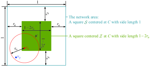
Figure 1: For the position of a node $v_{x}$ satisfying the condition that $v_{x}$’s distance to each edge of the unit square is at least $r_{n}$ with $r_{n}\leq\frac{1}{2}$, given the position of $v_{x}$, the conditional probability that another node $v_{y}$ falls in $v_{x}$’s transmission area is $\pi{r_{n}}^{2}$, since the circle centered at node $v_{x}$’s position with a radius of $r_{n}$ is completely inside the square.

On the other hand, whenever $v_{x}\not\in\mathcal{Z}$, the circle centered at node $v_{x}$’s position with a radius of $r_{n}$ may or may not be completely inside the square $\mathcal{S}$, so the probability that the random position of node $v_{y}$ belongs to the intersection of this circle and the square $\mathcal{S}$ is no greater than $\pi{r_{n}}^{2}$. Hence, given any location of $v_{x}$ which is outside of $\mathcal{Z}$, the conditional probability that $v_{x}$ and $v_{y}$ is at most $\pi{r_{n}}^{2}$, when we consider the uniform distribution of $v_{y}$’s position. Then the conditional probability of $\text{distance}(v_{x},v_{y})\leq r_{n}$ given $v_{x}\not\in\mathcal{Z}$ is no greater than $\pi{r_{n}}^{2}$, for $r_{n}\leq\frac{1}{2}$. Formally, we have

$$\textstyle{{\mathbb{P}}\left[{\big{(}\text{distance}(v_{x},v_{y})\leq r_{n}\big{)}\boldsymbol{\mid}(v_{x}\not\in\mathcal{Z})}\right]\leq\pi{r_{n}}^{2},\text{ for }r_{n}\leq\frac{1}{2}}.$$ (11)

Recall that $\mu_{n}(\mathcal{S})$ denotes $\text{distance}(v_{x},v_{y})\leq r_{n}$ on the unit square $\mathcal{S}$. Clearly, from the law of total probability, we derive

$$\mu_{n}(\mathcal{S})$$

$$={\mathbb{P}}\left[{\text{distance}(v_{x},v_{y})\leq r_{n}}\right]$$

$$={\mathbb{P}}\left[{\big{(}\text{distance}(v_{x},v_{y})\leq r_{n}\big{)}\hskip 2.0pt{\cap}\hskip 2.0pt(v_{x}\in\mathcal{Z})}\right]$$

$$\quad+{\mathbb{P}}\left[{\big{(}\text{distance}(v_{x},v_{y})\leq r_{n}\big{)}\hskip 2.0pt{\cap}\hskip 2.0pt(v_{x}\not\in\mathcal{Z})}\right]$$

$$={\mathbb{P}}\left[{\big{(}\text{distance}(v_{x},v_{y})\leq r_{n}\big{)}\boldsymbol{\mid}(v_{x}\in\mathcal{Z})}\right]\times{\mathbb{P}}\left[{v_{x}\in\mathcal{Z}}\right]$$

$$\quad+{\mathbb{P}}\left[{\big{(}\text{distance}(v_{x},v_{y})\leq r_{n}\big{)}\boldsymbol{\mid}(v_{x}\not\in\mathcal{Z})}\right]\times{\mathbb{P}}\left[{v_{x}\not\in\mathcal{Z}}\right].$$ (12)

Ignoring the term after the plus sign in (12), we further have

$$\mu_{n}(\mathcal{S}) \geq{\mathbb{P}}\left[{\big{(}\text{distance}(v_{x},v_{y})\leq r_{n}\big{)}\boldsymbol{\mid}(v_{x}\in\mathcal{Z})}\right]\times{\mathbb{P}}\left[{v_{x}\in\mathcal{Z}}\right].$$ (13)

Note that $v_{x}$ is uniformly distributed on the square $\mathcal{S}$, whose area denoted by $|\mathcal{S}|$ is given by $|\mathcal{S}|=1$. The square $\mathcal{Z}$ has a side length of $1-2r_{n}$, so its area denoted by $|\mathcal{Z}|$ equals $|\mathcal{Z}|=(1-2{r_{n}})^{2}$. Hence, we obtain

$${\mathbb{P}}\left[{v_{x}\in\mathcal{Z}}\right]=\frac{|\mathcal{Z}|}{|\mathcal{S}|}=\frac{(1-2{r_{n}})^{2}}{1}=(1-2{r_{n}})^{2},\text{ for }r_{n}\leq\textstyle{\frac{1}{2}},$$ (14)

and

$${\mathbb{P}}\left[{v_{x}\not\in\mathcal{Z}}\right]=1-{\mathbb{P}}\left[{v_{x}\in\mathcal{Z}}\right]=1-(1-2{r_{n}})^{2},\text{ for }r_{n}\leq\textstyle{\frac{1}{2}}.$$ (15)

Using (10) and (14) in (13), we get

$$\mu_{n}(\mathcal{S}) \geq\pi{r_{n}}^{2}\times(1-2{r_{n}})^{2},\text{ for }r_{n}\leq\textstyle{\frac{1}{2}}.$$ (16)

Applying (10) (11) (14) and (15) to (12), we establish

$$\mu_{n}(\mathcal{S}) \leq\pi{r_{n}}^{2}\times(1-2{r_{n}})^{2}+\pi{r_{n}}^{2}\times[1-(1-2{r_{n}})^{2}]$$

$$\leq\pi{r_{n}}^{2},\text{ for }r_{n}\leq\textstyle{\frac{1}{2}}.$$ (17)

Summarizing (16) and (17), we have $(1-2{r_{n}})^{2}\cdot\pi{r_{n}}^{2}\leq\mu_{n}(\mathcal{S})\leq\pi{r_{n}}^{2},\text{ for }r_{n}\leq\frac{1}{2}$; i.e., (8) is proved.

Proving (9) for $\mu_{n}(\mathcal{S})$ on the unit square $\mathcal{S}$: Recall that for two positive sequences $x_{n}$ and $y_{n}$, the relation $x_{n}\sim y_{n}$ means $\lim_{n\to\infty}\frac{x_{n}}{y_{n}}=1$. From (8), it follows that $(1-2{r_{n}})^{2}\leq\frac{\mu_{n}(\mathcal{S})}{\pi{r_{n}}^{2}}\leq 1,\text{ for }r_{n}\leq\frac{1}{2}$. Clearly, given $r_{n}=o(1)$, we have $\lim_{n\to\infty}(1-2{r_{n}})^{2}=1$ and also have $r_{n}\leq\frac{1}{2}$ for all $n$ sufficiently large. Summarizing the above results, we clearly obtain $\lim_{n\to\infty}\frac{\mu_{n}(\mathcal{S})}{\pi{r_{n}}^{2}}=1$; i.e., $\mu_{n}(\mathcal{S})\sim\pi{r_{n}}^{2}$. Hence, (9) is proved. $\blacksquare$

We now show results ①–③ of Page III.

We first show the above result ①. By [43, Lemma 1], if $K_{n}=\omega(1)$ and $K_{n}=o\big{(}\sqrt{P_{n}}\big{)}$, then

$$\textstyle{p_{q}\sim\frac{1}{q!}\cdot\frac{{K_{n}}^{2q}}{{P_{n}}^{q}}}.$$ (18)

The asymptotic equivalence (18) above holds for $\textnormal{network}^{\textnormal{full visibility}}$ under condition set $\Lambda$ in (6) on Page 6, since we have $K_{n}=\omega(1)$ and $K_{n}=o\big{(}\sqrt{P_{n}}\big{)}$ from $\Lambda$.

We then explain the result ②. With $\mu_{n}(\mathcal{T})$ (resp., $\mu_{n}(\mathcal{S})$) denoting the probability that two nodes are within distance $r_{n}$ when they are independently and uniformly distributed on the unit torus $\mathcal{T}$ (resp., the unit square $\mathcal{S}$), Lemma 1 above shows $\textstyle{\mu_{n}(\mathcal{T})=\pi{r_{n}}^{2},\text{ for }r_{n}\leq\frac{1}{2}}$, and $\mu_{n}(\mathcal{S})\sim\pi{r_{n}}^{2},\text{ for }r_{n}=o(1)$. We can use Lemma 1 because our condition set $\Lambda$ in (6) on Page 6 has the condition $r_{n}=o(1)$, which implies $r_{n}\leq\frac{1}{2}$ for all $n$ sufficiently large. In words, Lemma 1 says that the probability that two nodes are within distance $r_{n}$ is given by $\pi{r_{n}}^{2}$ on the unit torus $\mathcal{T}$, and is asymptotically equivalent to $\pi{r_{n}}^{2}$ on the unit square $\mathcal{S}$. In each of $\textnormal{static-network}^{\textnormal{disk model}}_{\textnormal{unit torus}}$ and $\textnormal{static-network}^{\textnormal{disk model}}_{\textnormal{unit square}}$, since two nodes have an edge in between if and only if they are within distance $r_{n}$ and also they share at least $q$ keys, then under condition set $\Lambda$, the edge probability is asymptotically equivalent to $\frac{1}{q!}\cdot\frac{{K_{n}}^{2q}}{{P_{n}}^{q}}\cdot\pi{r_{n}}^{2}$ from $\mu_{n}(\mathcal{T})=\pi{r_{n}}^{2}$, $\mu_{n}(\mathcal{S})\sim\pi{r_{n}}^{2}$ and $p_{q}\sim\frac{1}{q!}\cdot\frac{{K_{n}}^{2q}}{{P_{n}}^{q}}$ in (18). Furthermore, at each time slot, mobile networks $\textnormal{mobile-network}^{\textnormal{disk model}}_{\textnormal{unit torus}}$ and $\textnormal{mobile-network}^{\textnormal{disk model}}_{\textnormal{unit square}}$ can be viewed as instances of static networks $\textnormal{static-network}^{\textnormal{disk model}}_{\textnormal{unit torus}}$ and $\textnormal{static-network}^{\textnormal{disk model}}_{\textnormal{unit square}}$, respectively. In view of the above, the result ② is proved.

We now show the result ③. Compared with the networks in the result ②, the networks in the result ③ also consider link unreliability, in which each link is allowed to be inactive with probability $t_{n}$. Multiplying the term $\frac{1}{q!}\cdot\frac{{K_{n}}^{2q}}{{P_{n}}^{q}}\cdot\pi{r_{n}}^{2}$ with $t_{n}$, we obtain $\frac{1}{q!}\cdot\frac{{K_{n}}^{2q}}{{P_{n}}^{q}}\cdot\pi{r_{n}}^{2}\cdot t_{n}$, which is a common asymptotic value of the edge probabilities of the networks in the result ③. Therefore, the result ③ follows.

We have shown the results ① ② and ③ on the asymptotic values of the edge probabilities of the networks in Table III. For each network in Table III, let $\widetilde{\textnormal{edge-prob}}$ denote the used asymptotic value of its edge probability; namely, $\widetilde{\textnormal{edge-prob}}$ is $\frac{1}{q!}\cdot\frac{{K_{n}}^{2q}}{{P_{n}}^{q}}$ for $\textnormal{network}^{\textnormal{full visibility}}$ in the result ①, is $\frac{1}{q!}\cdot\frac{{K_{n}}^{2q}}{{P_{n}}^{q}}\cdot\pi{r_{n}}^{2}$ for the four networks in the result ②, and is $\frac{1}{q!}\cdot\frac{{K_{n}}^{2q}}{{P_{n}}^{q}}\cdot\pi{r_{n}}^{2}\cdot t_{n}$ for the four networks in the result ③. As given in Table III, the conditions related to $\frac{\ln n}{n}$ can be summarized as follows. For $\textnormal{network}^{\textnormal{full visibility}}$ and the four networks on the unit torus, we have the condition that $\widetilde{\textnormal{edge-prob}}\geq\frac{c\ln n}{n}$ for any constant $c>1$. For the four networks on the unit square, we have the condition that $\widetilde{\textnormal{edge-prob}}\geq\frac{c\ln n}{n}$ for any constant $c>\widetilde{c}_{n}$, where $\widetilde{c}_{n}$ is given by

$$\widetilde{c}_{n}:=\max\bigg{\{}1+\Big{(}\ln\big{[}(\widetilde{\textnormal{edge-prob}})^{-1}\big{]}\Big{)}\bigg{/}\ln n,$$

$$\quad\quad\quad\quad\quad\quad\quad 4\Big{(}\ln\big{[}(\widetilde{\textnormal{edge-prob}})^{-1}\big{]}\Big{)}\bigg{/}\ln n\bigg{\}}$$

$$=\begin{cases}1+\Big{(}\ln\big{[}(\widetilde{\textnormal{edge-prob}})^{-1}\big{]}\Big{)}\bigg{/}\ln n,\textnormal{ if }\widetilde{\textnormal{edge-prob}}=\widetilde{\Omega}(n^{-1/3}),\\ 4\Big{(}\ln\big{[}(\widetilde{\textnormal{edge-prob}})^{-1}\big{]}\Big{)}\bigg{/}\ln n,\textnormal{ if }\widetilde{\textnormal{edge-prob}}=\widetilde{O}(n^{-1/3}).\end{cases}$$ (19)

In (19) above, we write a quantity $x_{n}$ as $\widetilde{\Omega}(n^{\alpha})$ for some constant $\alpha$ if $x_{n}\geq n^{\alpha-\epsilon_{1}}$ for all $n$ sufficiently large, where $\epsilon_{1}$ is an arbitrary positive constant. Similarly, a quantity $x_{n}$ is written as $\widetilde{O}(n^{\alpha})$ for some constant $\alpha$ if $x_{n}\leq n^{\alpha+\epsilon_{2}}$ for all $n$ sufficiently large, where $\epsilon_{2}$ is an arbitrary positive constant.

The difference between the condition $c>1$ for networks on the torus, and the condition $c>\widetilde{c}_{n}$ for networks on the square is resulted from the boundary effect of the square.

From (19), we observe a phase transition of $\widetilde{c}_{n}$ when $\widetilde{\textnormal{edge-prob}}$ or the edge probability asymptotically changes from $\widetilde{\Omega}(n^{-1/3})$ to $\widetilde{O}(n^{-1/3})$, or vice versa. The intuition is that to compute the expected number of isolated nodes, in integrating all possible points in unit square $\mathcal{S}$ with the boundary effect, different areas on $\mathcal{S}$ contribute to the dominant part of the integral depending on the edge probability, where a node is non-isolated if it has a link with at least another node, and a node is isolated if it has no link with any other node.

We now present the connectivity results in Table III as more understandable theorems, which are all proved in Section VI. We give first the results of secure sensor networks under full visibility, then the results of static secure sensor networks, and finally those of mobile secure sensor networks. As mentioned before in Section III for the system model, all studied networks employ the $q$-composite scheme.

IV-A1 Connectivity of Secure Sensor Networks with the $q$-Composite Scheme under Full Visibility

Theorem 1 below on connectivity is for the full visibility case. Its proof is provided in Section VI-A.

Theorem 1 (Connectivity of $\textnormal{network}^{\textnormal{full visibility}}$).

Under condition set $\Lambda$ in (6) on Page 6, a secure sensor network with the $q$-composite scheme under full visibility is connected with high probability if $\frac{1}{q!}\cdot\frac{{K_{n}}^{2q}}{{P_{n}}^{q}}\geq\frac{c\ln n}{n}$ for all $n$ sufficiently large, where $c$ is a constant with $c>1$.

As explained in the result ① in Section IV-A, $\frac{1}{q!}\cdot\frac{{K_{n}}^{2q}}{{P_{n}}^{q}}$ is an asymptotic value of the edge probability of $\textnormal{network}^{\textnormal{full visibility}}$. Although Theorem 1 can also be derived using the results in [30], the proof techniques in [30] lack formality (specifically [30, Equation (6.93)]) and are different from those in this paper. In addition, Bloznelis and Rybarczyk [29] (resp., Bloznelis and Łuczak [10]) have recently investigated connectivity (resp., $k$-connectivity) of $\textnormal{network}^{\textnormal{full visibility}}$, but both results after a rewriting address only the narrow and impractical range of $P_{n}=o\big{(}n^{\frac{1}{q}}(\ln n)^{-\frac{3}{5q}}\big{)}$. In contrast, from condition set $\Lambda$ in (6), our Theorem 1 considers a more practical range of $P_{n}=\omega(n\ln n)$. More details can be found in Section II for related work.

IV-A2 Connectivity of Static Secure Sensor Networks with the $q$-Composite Scheme

Theorems 2–5 present connectivity results of static secure sensor networks. Their proofs are deferred to Section VI-B.

IV-A2a Connectivity under the Disk Model on the Torus without the Boundary Effect

Theorem 2 (Connectivity of $\textnormal{static-network}^{\textnormal{disk model}}_{\textnormal{unit torus}}$).

Under condition set $\Lambda$ in (6) on Page 6, a static secure sensor network with the $q$-composite scheme under the disk model on the unit torus without the boundary effect is connected with high probability if $\frac{1}{q!}\cdot\frac{{K_{n}}^{2q}}{{P_{n}}^{q}}\cdot\pi{r_{n}}^{2}\geq\frac{c\ln n}{n}$ for all $n$ sufficiently large, where $c$ is a constant with $c>1$.

As given in the result ② in Section IV-A, $\frac{1}{q!}\cdot\frac{{K_{n}}^{2q}}{{P_{n}}^{q}}\cdot\pi{r_{n}}^{2}$ is asymptotically equivalent to the edge probability of $\textnormal{static-network}^{\textnormal{disk model}}_{\textnormal{unit torus}}$.

IV-A2b Connectivity with Unreliable Links under the Disk Model on the Torus without the Boundary Effect

Theorem 3 (Connectivity of $\textnormal{static-network}^{\begin{subarray}{\textnormal{missing}}{\textnormal{disk model}}\\ \textnormal{unit torus}\end{subarray}}_{\textnormal{unreliable links}}$).

Under condition set $\Lambda$ in (6) on Page 6, a static secure sensor network with the $q$-composite scheme and unreliable links under the disk model on the unit torus without the boundary effect is connected with high probability if $\frac{1}{q!}\cdot\frac{{K_{n}}^{2q}}{{P_{n}}^{q}}\cdot\pi{r_{n}}^{2}\cdot t_{n}\geq\frac{c\ln n}{n}$ for all $n$ sufficiently large, where $c$ is a constant with $c>1$.

As explained in the result ③ in Section IV-A, $\frac{1}{q!}\cdot\frac{{K_{n}}^{2q}}{{P_{n}}^{q}}\cdot\pi{r_{n}}^{2}\cdot t_{n}$ is an asymptotic value of the edge probability of $\textnormal{static-network}^{\begin{subarray}{\textnormal{missing}}{\textnormal{disk model}}\\ \textnormal{unit torus}\end{subarray}}_{\textnormal{unreliable links}}$.

IV-A2c Connectivity under the Disk Model on the Square with the Boundary Effect

Theorem 4 (Connectivity of $\textnormal{static-network}^{\textnormal{disk model}}_{\textnormal{unit square}}$).

Under condition set $\Lambda$ in (6) on Page 6, a static secure sensor network with the $q$-composite scheme under the disk model on the unit square with the boundary effect is connected with high probability if $\frac{1}{q!}\cdot\frac{{K_{n}}^{2q}}{{P_{n}}^{q}}\cdot\pi{r_{n}}^{2}\geq\frac{c\ln n}{n}$ for all $n$ sufficiently large, where $c$ is some constant satisfying for all $n$ sufficiently large that

$$c>c_{n}^{*}:=\max\bigg{\{}1+\bigg{(}\ln\frac{P_{n}}{{K_{n}}^{2}}\bigg{)}\bigg{/}\ln n,\hskip 2.0pt4\bigg{(}\ln\frac{P_{n}}{{K_{n}}^{2}}\bigg{)}\bigg{/}\ln n\bigg{\}}.$$ (20)

As given in the result ② in Section IV-A, $\frac{1}{q!}\cdot\frac{{K_{n}}^{2q}}{{P_{n}}^{q}}\cdot\pi{r_{n}}^{2}$ is asymptotically equivalent to the edge probability of $\textnormal{static-network}^{\textnormal{disk model}}_{\textnormal{unit square}}$.

IV-A2d Connectivity with Unreliable Links under the Disk Model on the Square with the Boundary Effect

Theorem 5 (Connectivity of $\textnormal{static-network}^{\begin{subarray}{\textnormal{missing}}{\textnormal{disk model}}\\ \textnormal{unit square}\end{subarray}}_{\textnormal{unreliable links}}$).

Under condition set $\Lambda$ in (6) on Page 6, a static secure sensor network with the $q$-composite scheme and unreliable links under the disk model on the unit square with the boundary effect is connected with high probability if $\frac{1}{q!}\cdot\frac{{K_{n}}^{2q}}{{P_{n}}^{q}}\cdot\pi{r_{n}}^{2}\cdot t_{n}\geq\frac{c\ln n}{n}$ for all $n$ sufficiently large, where $c$ is some constant satisfying for all $n$ sufficiently large that

$$c>c_{n}^{\#}:=\max\bigg{\{}1+\bigg{(}q\ln\frac{P_{n}}{{K_{n}}^{2}}+\ln\frac{1}{t_{n}}\bigg{)}\bigg{/}\ln n,$$

$$~{}~{}~{}~{}~{}~{}~{}~{}~{}~{}~{}~{}~{}~{}~{}~{}~{}~{}~{}~{}~{}~{}~{}~{}~{}4\bigg{(}q\ln\frac{P_{n}}{{K_{n}}^{2}}+\ln\frac{1}{t_{n}}\bigg{)}\bigg{/}\ln n\bigg{\}}.$$ (21)

As explained in the result ③ in Section IV-A, $\frac{1}{q!}\cdot\frac{{K_{n}}^{2q}}{{P_{n}}^{q}}\cdot\pi{r_{n}}^{2}\cdot t_{n}$ is an asymptotic value of the edge probability of $\textnormal{static-network}^{\begin{subarray}{\textnormal{missing}}{\textnormal{disk model}}\\ \textnormal{unit square}\end{subarray}}_{\textnormal{unreliable links}}$.

IV-A3 Connectivity of Mobile Secure Sensor Networks with the $q$-Composite Scheme

Theorems 6–9 below present connectivity results of mobile secure sensor networks. Their proofs are deferred to Section VI-C. As explained in Section III for the system model, at each time slot, each mobile network can be viewed as an instance of its corresponding static network, and thus its edge probability defined for each time slot also equals that of the corresponding static network.

IV-A3a Connectivity under the Disk Model on the Torus without the Boundary Effect

Theorem 6 (Connectivity of $\textnormal{mobile-network}^{\textnormal{disk model}}_{\textnormal{unit torus}}$).

Under condition set $\Lambda$ in (6) on Page 6, a mobile secure sensor network with the $q$-composite scheme under the disk model on the unit torus without the boundary effect and under the i.i.d. mobility model is connected with high probability for at least $n^{c-1-\epsilon}$ consecutive time slots from the beginning for an arbitrary positive constant $\epsilon$, if $\frac{1}{q!}\cdot\frac{{K_{n}}^{2q}}{{P_{n}}^{q}}\cdot\pi{r_{n}}^{2}\geq\frac{c\ln n}{n}$ for all $n$ sufficiently large, where $c$ is a constant with $c>1$.

As given in the result ② in Section IV-A, $\frac{1}{q!}\cdot\frac{{K_{n}}^{2q}}{{P_{n}}^{q}}\cdot\pi{r_{n}}^{2}$ is asymptotically equivalent to the edge probability of $\textnormal{mobile-network}^{\textnormal{disk model}}_{\textnormal{unit torus}}$. Also, from Theorem 2, the conditions in Theorem 6 also ensure that the corresponding static network $\textnormal{static-network}^{\textnormal{disk model}}_{\textnormal{unit torus}}$ is connected with high probability.

IV-A3b Connectivity with Unreliable Links under the Disk Model on the Torus without the Boundary Effect

Theorem 7 (Connectivity of $\textnormal{mobile-network}^{\begin{subarray}{\textnormal{missing}}{\textnormal{disk model}}\\ \textnormal{unit torus}\end{subarray}}_{\textnormal{unreliable links}}$).

Under condition set $\Lambda$ in (6) on Page 6, a mobile secure sensor network with the $q$-composite scheme and unreliable links under the disk model on the unit torus without the boundary effect and under the i.i.d. mobility model is connected with high probability for at least $n^{c-1-\epsilon}$ consecutive time slots from the beginning for an arbitrary positive constant $\epsilon$, if $\frac{1}{q!}\cdot\frac{{K_{n}}^{2q}}{{P_{n}}^{q}}\cdot\pi{r_{n}}^{2}\cdot t_{n}\geq\frac{c\ln n}{n}$ for all $n$ sufficiently large, where $c$ is a constant with $c>1$.

As explained in the result ③ in Section IV-A, $\frac{1}{q!}\cdot\frac{{K_{n}}^{2q}}{{P_{n}}^{q}}\cdot\pi{r_{n}}^{2}\cdot t_{n}$ is an asymptotic value of the edge probability of $\textnormal{mobile-network}^{\begin{subarray}{\textnormal{missing}}{\textnormal{disk model}}\\ \textnormal{unit torus}\end{subarray}}_{\textnormal{unreliable links}}$. Moreover, from Theorem 3, the conditions in Theorem 7 also ensure that the corresponding static network $\textnormal{static-network}^{\begin{subarray}{\textnormal{missing}}{\textnormal{disk model}}\\ \textnormal{unit torus}\end{subarray}}_{\textnormal{unreliable links}}$ is connected with high probability.

IV-A3c Connectivity under the Disk Model on the Square with the Boundary Effect

Theorem 8 (Connectivity of $\textnormal{mobile-network}^{\textnormal{disk model}}_{\textnormal{unit square}}$).

Under condition set $\Lambda$ in (6) on Page 6, a mobile secure sensor network with the $q$-composite scheme under the disk model on the unit square with the boundary effect and under the i.i.d. mobility model is connected with high probability for at least $n^{c-c_{n}^{*}-\epsilon}$ consecutive time slots from the beginning for an arbitrary positive constant $\epsilon$, if $\frac{1}{q!}\cdot\frac{{K_{n}}^{2q}}{{P_{n}}^{q}}\cdot\pi{r_{n}}^{2}\geq\frac{c\ln n}{n}$ for all $n$ sufficiently large, where $c$ is some constant satisfying $c>c_{n}^{*}$ for all $n$ sufficiently large, with $c_{n}^{*}$ defined in (20).

As given in the result ② in Section IV-A, $\frac{1}{q!}\cdot\frac{{K_{n}}^{2q}}{{P_{n}}^{q}}\cdot\pi{r_{n}}^{2}$ is asymptotically equivalent to the edge probability of $\textnormal{mobile-network}^{\textnormal{disk model}}_{\textnormal{unit square}}$. In addition, from Theorem 4, the conditions in Theorem 8 also ensure that the corresponding static network $\textnormal{static-network}^{\textnormal{disk model}}_{\textnormal{unit square}}$ is connected with high probability.

IV-A3d Connectivity with Unreliable Links under the Disk Model on the Square with the Boundary Effect

Theorem 9 (Connectivity of $\textnormal{mobile-network}^{\begin{subarray}{\textnormal{missing}}{\textnormal{disk model}}\\ \textnormal{unit square}\end{subarray}}_{\textnormal{unreliable links}}$).

Under condition set $\Lambda$ in (6) on Page 6, a mobile secure sensor network with the $q$-composite scheme and unreliable links under the disk model on the unit square with the boundary effect and under the i.i.d. mobility model is connected with high probability for at least $n^{c-c_{n}^{\#}-\epsilon}$ consecutive time slots from the beginning for an arbitrary positive constant $\epsilon$, if $\frac{1}{q!}\cdot\frac{{K_{n}}^{2q}}{{P_{n}}^{q}}\cdot\pi{r_{n}}^{2}\cdot t_{n}\geq\frac{c\ln n}{n}$ for all $n$ sufficiently large, where $c$ is some constant satisfying $c>c_{n}^{\#}$ for all $n$ sufficiently large, with $c_{n}^{\#}$ defined in (21).

As explained in the result ③ in Section IV-A, $\frac{1}{q!}\cdot\frac{{K_{n}}^{2q}}{{P_{n}}^{q}}\cdot\pi{r_{n}}^{2}\cdot t_{n}$ is an asymptotic value of the edge probability of $\textnormal{mobile-network}^{\begin{subarray}{\textnormal{missing}}{\textnormal{disk model}}\\ \textnormal{unit square}\end{subarray}}_{\textnormal{unreliable links}}$. Furthermore, from Theorem 5, the conditions in Theorem 9 also ensure that the corresponding static network $\textnormal{static-network}^{\begin{subarray}{\textnormal{missing}}{\textnormal{disk model}}\\ \textnormal{unit square}\end{subarray}}_{\textnormal{unreliable links}}$ is connected with high probability.

IV-A4 Connectivity under Random Node-Capture Attacks

We present below the connectivity results under random node-capture attacks. After the adversary has captured some random set of $m$ nodes, the remaining network is statistically equivalent to a network initially with $(n-m)$ nodes in the absence of node capture. Hence, by replacing $\ln n$ with $\ln(n-m)$, replacing $\frac{\ln n}{n}$ with $\frac{\ln(n-m)}{n-m}$ and $n$ with $(n-m)$ in the connectivity results in Table III, we obtain the connectivity results in Table IV for an $n$-size network after the adversary has captured a random set of $m$ nodes out of all $n$ nodes. Note that we do not replace the “$n$” in $K_{n}$, $P_{n}$, $r_{n}$, $t_{n}$.

Settings			Connectivity results under a random capture of $m$ nodes
static/mobile secure sensor networks under full visibility			connected if $\frac{1}{q!}\cdot\frac{{K_{n}}^{2q}}{{P_{n}}^{q}}\geq\frac{c\ln(n-m)}{n-m}$ for any constant $c>1$
static secure sensor networks	disk model	torus	connected if $\frac{1}{q!}\cdot\frac{{K_{n}}^{2q}}{{P_{n}}^{q}}\cdot\pi{r_{n}}^{2}\geq\frac{c\ln(n-m)}{n-m}$ for any constant $c>1$
		square	connected if $\frac{1}{q!}\cdot\frac{{K_{n}}^{2q}}{{P_{n}}^{q}}\cdot\pi{r_{n}}^{2}\geq\frac{c\ln(n-m)}{n-m}$ for any constant $c>c_{n}^{*}$
	disk model w/ unreliable links	torus	connected if $\frac{1}{q!}\cdot\frac{{K_{n}}^{2q}}{{P_{n}}^{q}}\cdot\pi{r_{n}}^{2}\cdot t_{n}\geq\frac{c\ln(n-m)}{n-m}$ for any constant $c>1$
		square	connected if $\frac{1}{q!}\cdot\frac{{K_{n}}^{2q}}{{P_{n}}^{q}}\cdot\pi{r_{n}}^{2}\cdot t_{n}\geq\frac{c\ln(n-m)}{n-m}$ for any constant $c>c_{n}^{\#}$
mobile secure sensor networks	disk model	torus	connected for at least $(n-m)^{c-1-\epsilon}$ consecutive time slots if $\frac{1}{q!}\cdot\frac{{K_{n}}^{2q}}{{P_{n}}^{q}}\cdot\pi{r_{n}}^{2}\geq\frac{c\ln(n-m)}{n-m}$ for any constant $c>1$
		square	connected for at least $(n-m)^{c-c_{n}^{*}-\epsilon}$ consecutive time slots if $\frac{1}{q!}\cdot\frac{{K_{n}}^{2q}}{{P_{n}}^{q}}\cdot\pi{r_{n}}^{2}\geq\frac{c\ln(n-m)}{n-m}$ for any constant $c>c_{n}^{*}$
	disk model w/ unreliable links	torus	connected for at least $(n-m)^{c-1-\epsilon}$ consecutive time slots if $\frac{1}{q!}\cdot\frac{{K_{n}}^{2q}}{{P_{n}}^{q}}\cdot\pi{r_{n}}^{2}\cdot t_{n}\geq\frac{c\ln(n-m)}{n-m}$ for any constant $c>1$
		square	connected for at least $(n-m)^{c-c_{n}^{\#}-\epsilon}$ consecutive time slots if $\frac{1}{q!}\cdot\frac{{K_{n}}^{2q}}{{P_{n}}^{q}}\cdot\pi{r_{n}}^{2}\cdot t_{n}\geq\frac{c\ln(n-m)}{n-m}$ for any constant $c>c_{n}^{\#}$

TABLE IV: Different settings of secure sensor networks and their connectivity results under a random capture of $m$ nodes, where “w/” is short for “with”. Note that $c_{n}^{*}$ is $\max\Big{\{}1+\big{(}\ln\frac{P_{n}}{{K_{n}}^{2}}\big{)}\big{/}[\ln(n-m)],~{}4\big{(}\ln\frac{P_{n}}{{K_{n}}^{2}}\big{)}\big{/}[\ln(n-m)]\Big{\}}$, $c_{n}^{\#}$ is $\max\Big{\{}1+\big{(}q\ln\frac{P_{n}}{{K_{n}}^{2}}+\ln\frac{1}{t_{n}}\big{)}\big{/}[\ln(n-m)],~{}4\big{(}q\ln\frac{P_{n}}{{K_{n}}^{2}}+\ln\frac{1}{t_{n}}\big{)}\big{/}[\ln(n-m)]\Big{\}}$, and $\epsilon$ is an arbitrary positive constant. All results are in the asymptotic sense to hold with high probability, and thus the conditions in the table only need to hold for all $n$ sufficiently large. Except the result under full visibility which requires conditions on $K_{n}$ and $P_{n}$ in condition set $\Lambda$ in (6) on Page 6 but not the condition $r_{n}=o(1)$ in $\Lambda$, all other results need the whole condition set $\Lambda$.

IV-B Unsplittability of Secure Sensor Networks with the $q$-Composite Scheme

Recall the definition of unsplittability in Section I-B. A secure sensor network is unsplittable if with high probability an adversary that has captured an arbitrary set of $o(n)$ sensors cannot partition the network into two chunks, which both have linear sizes of sensors, and either are isolated from each other or only have compromised communications in between.

IV-B1 Unsplittability under Full Visibility

Theorem 10.

A secure sensor network with the $q$-composite scheme under full visibility is unsplittable with high probability if $\frac{1}{q!}\cdot\frac{{K_{n}}^{2q}}{{P_{n}}^{q}}\geq\frac{c\ln n}{n}$ for any constant $c>1$, $K_{n}=\omega(\ln n)$ and $K_{n}=o\big{(}\min\{\sqrt{P_{n}},\frac{P_{n}}{n}\}\big{)}$.

By Theorem 1, the conditions in Theorem 10 also ensure that a secure sensor network with the $q$-composite scheme under full visibility is connected with high probability. Intuitively, these conditions to guarantee connectivity in the absence of node capture can also ensure that when $o(n)$ nodes are compromised, almost all of the remaining nodes are still securely connected. More formally, the idea to show Theorem 1 is that even if $n_{1}=o(n)$ nodes are compromised, we still have a securely connected network consisting of $n-n_{2}$ nodes, where $n_{2}$ can also be written as $o(n)$ despite $n_{2}\geq n_{1}$. The reason for $n_{2}\geq n_{1}$ is that capturing nodes enables an adversary to compromise communications between non-captured nodes which happen to use keys that are also shared by captured nodes.

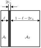
Figure 2: An adversary that has captured all $o(n)$ nodes in the shaded region can partition the network into two chunks $\mathcal{A}_{1}$ and $\mathcal{A}_{2}$, which both have linear sizes of sensors with high probability and are isolated from each other. We let $\ell$ be a constant with $0<\ell<1$, and consider $r_{n}=o(1)$.

IV-B2 Unsplittability under the Disk Model

Theorem 11.

A static secure sensor network with the $q$-composite scheme under the disk model on the unit torus or unit square is splittable with high probability if $r_{n}=o(1)$.

To explain Theorem 11, Figure 2 illustrates that an adversary capturing all $o(n)$ nodes in the shaded region can partition the network into two chunks $\mathcal{A}_{1}$ and $\mathcal{A}_{2}$, which both have linear sizes of sensors with high probability and are isolated from each other. We present the specific details below for an intuitive understanding, and provide the technical proofs in Section VI-E. First, under $r_{n}=o(1)$, we show that the number of nodes in the shaded region (i.e., a rectangle of width $2r_{n}$ and length $1$) contains $o(n)$ nodes with high probability since the area of this region is also $o(1)$. Furthermore, because $\ell$ in Figure 2 is a constant with $0<\ell<1$, the areas of chunks $\mathcal{A}_{1}$ and $\mathcal{A}_{2}$ are both constants, which enable us to prove that each chunk has $\Theta(n)$ nodes (i.e., a constant fraction of the $n$ nodes) with high probability. Finally, it is clear that any node in region $\mathcal{A}_{1}$ and any node in region $\mathcal{A}_{2}$ have a distance at least $2r_{n}$, so the node set in $\mathcal{A}_{1}$ and the node set in $\mathcal{A}_{2}$ have no edge in between.

IV-C Unassailability of Secure Sensor Networks with the $q$-Composite Scheme

Many prior studies have analyzed node-captured attacks, but they often consider that the adversary randomly captures sensors. However, in practice, the adversary may tune its node-capture strategy according to its goal. To analyze unassailability, we consider arbitrary node-capture attacks, in which the adversary can capture an arbitrary set of sensors. Recalling the definition of unassailability in Section I-B, a secure sensor network is unassailable if an adversary that has captured an arbitrary set of $o(n)$ sensors can compromise only $o(1)$ fraction of communication links in the rest of the network; in other words, an adversary has to capture a constant fraction of sensors to compromise a constant fraction of communication links. For the $q$-composite scheme, previous studies have considered random node-capture attacks, but not arbitrary node-capture attacks formally. Hence, no prior work has rigorously established the parameter conditions under which secure sensor networks with the $q$-composite scheme are unassailable. Our Theorem 12 below presents the condition for unassailability of the $q$-composite scheme.

Theorem 12.

A secure sensor network with the $q$-composite scheme under any communication model is unassailable with high probability under ${P_{n}}/{K_{n}}=\Omega(n)$.

Under a different setting, a result similar to Theorem 12 is given in [17, 18], but the result of [17, 18] is not for unassailability which by definition considers arbitrary node-capture attacks. Specifically, [17, 18] considers only random node capture where the adversary captures a random set of $m$ sensors, whereas this paper addresses arbitrary node capture where the adversary captures an arbitrary set of $m$ sensors. The choice of $m$ nodes depends on the adversary’s goal and also physical limitations (e.g., some sensors may be easier to be captured than others). Theorem 12 is proved in Section VI-F.

We check the practicality of ${P_{n}}/{K_{n}}=\Omega(n)$ in Theorem 12. Recall that the key ring size $K_{n}$ denotes the number of keys in each sensor’s memory and $P_{n}$ means the key pool size which the keys on each sensor are selected from. In real-world sensor networks implementations, $K_{n}$ is several orders of magnitude smaller than $n$ due to limited memory and computational capability of sensors, and $P_{n}$ is larger than $n$ [2, 1, 4]. Thus, condition ${P_{n}}/{K_{n}}=\Omega(n)$ is practical.

To find the optimal $q$ that defends against node-capture attacks, we will investigate how $p_{\textnormal{compromised}}$ changes with respect to $q$. Since $p_{\textnormal{compromised}}$ depends on the capture strategy, to study how $p_{\textnormal{compromised}}$ varies with respect to $q$, below we consider the special case where the adversary captures a random set of $m$ sensors. This has been studied in [17], but here we will improve the results of [17]. We state the research question more precisely as follows: given $n$, if we fix the key ring size $K_{n}$ and the key-setup probability $p_{q}$, and vary $q$, the required amount of key overlap, how does the probability $p_{\textnormal{compromised}}$ change asymptotically with respect to $q$?

To answer the above question, we first explain the key-setup probability $p_{q}$ below. In the $q$-composite scheme, noting that all sensors’ key rings are random variables following the same probability distribution, we define the key-setup probability $p_{q}$ as the probability that the key rings of two sensors have at least $q$ keys in common. More specifically, with $\{v_{1},v_{2},\ldots,v_{n}\}$ denoting the set of $n$ sensors in the network, and with $R_{\ell}$ denoting the key ring of sensor $v_{\ell}$ for $\ell=1,2,\ldots,n$, then we have the same value of $\mathbb{P}[|R_{i}\cap R_{j}|\geq q]$ for each pair of different $i,j$ since each $R_{\ell}$ is constructed by selecting $K_{n}$ keys uniformly at random from the key pool $\mathcal{P}_{n}$ of $P_{n}$ keys. This value is denoted by $p_{q}$. Similarly, given $u$, we have the same value of $\mathbb{P}[|R_{i}\cap R_{j}|=u]$ for each pair of different $i,j$ so we define $\rho_{u}$ as $\mathbb{P}[|R_{i}\cap R_{j}|=u]$; i.e., $\rho_{u}$ is the probability that two nodes $v_{i}$ and $v_{j}$ share $u$ keys exactly in their key rings. Then we have $p_{q}=\mathbb{P}[|R_{i}\cap R_{j}|\geq q]=\sum_{u=q}^{K_{n}}\mathbb{P}[|R_{i}\cap R_{j}|=u]=\sum_{u=q}^{K_{n}}\rho_{u}$, where $\rho_{u}$ denoting $\mathbb{P}[|R_{i}\cap R_{j}|=u]$ can be computed as follows. After $R_{i}$ comprising $K_{n}$ keys is chosen from the key pool $\mathcal{P}_{n}$ of $P_{n}$ keys, to have $|R_{i}\cap R_{j}|=u$ with $R_{j}$ of $K_{n}$ keys choosing from $\mathcal{P}_{n}$, we need to select $u$ keys from $R_{i}$ and $(K_{n}-u)$ keys from $\mathcal{P}_{n}\setminus R_{i}$ to construct $R_{j}$, which gives $\binom{K_{n}}{u}\binom{P_{n}-K_{n}}{K_{n}-u}$ possibilities of $R_{j}$. Without $|R_{i}\cap R_{j}|=u$, we have $\binom{P_{n}}{K_{n}}$ possible ways to find $K_{n}$ keys from $\mathcal{P}_{n}$ to form $R_{j}$. Given the above, we have

$$\rho_{u}=\mathbb{P}[|R_{i}\cap R_{j}|=u] =\frac{\binom{K_{n}}{u}\binom{P_{n}-K_{n}}{K_{n}-u}}{\binom{P_{n}}{K_{n}}}$$ (22)

and

$$p_{q}=\mathbb{P}[|R_{i}\cap R_{j}|\geq q] =\sum_{u=q}^{K_{n}}\frac{\binom{K_{n}}{u}\binom{P_{n}-K_{n}}{K_{n}-u}}{\binom{P_{n}}{K_{n}}}.$$ (23)

From (23), $p_{q}$ is a function of the parameters $K_{n},P_{n}$ and $q$. Hence, to fix $p_{q}$, the key pool size $P_{n}$ needs to decrease as $q$ increases.

We now present Theorem 13 below, which gives the optimal $q$ that defends against node-capture attacks.

Theorem 13.

In a secure sensor network with the $q$-composite scheme under any communication model, if the key ring size $K_{n}$ and the key-setup probability $p_{q}$ are both fixed, and conditions $K_{n}=\omega(1)$ and $K_{n}=o\big{(}\sqrt{P_{n}}\big{)}$ hold, after an adversary has captured $m$ sensors with $m=o\Big{(}\sqrt{\frac{P_{n}}{{K_{n}}^{2}}}\hskip 2.0pt\Big{)}$, then the fraction of communications compromised in the rest of the network asymptotically achieves its minimum

• at $q=1$ if $\frac{K_{n}}{m}<2$,

• at both $q=1$ and $q=2$ if $\frac{K_{n}}{m}=2$,

• at $q=\big{\lfloor}{K_{n}}/{m}\big{\rfloor}$ if $\frac{K_{n}}{m}>2$ and ${K_{n}}/{m}$ is not an integer, and

• at both $q={K_{n}}/{m}$ and $q=({K_{n}}/{m})-1$ if ${K_{n}}/{m}$ is an integer greater than $2$.

Theorem 13 improves the result of [17], and is proved in Section VI-G.

IV-D Design guidelines for secure sensor networks

Based on our theorems above, we can provide design guidelines of secure sensor networks to achieve desired resilience and connectivity. We first take $\textnormal{static-network}^{\textnormal{disk model}}_{\textnormal{unit torus}}$ as an example.

From Theorems 2 and 12, for $\textnormal{static-network}^{\textnormal{disk model}}_{\textnormal{unit torus}}$, to ensure i) the network is resilient in the sense that an adversary capturing sensors at random has to obtain at least a constant fraction of nodes of the network in order to compromise a constant fraction of secure links, and ii) the network is connected with high probability, we can enforce ${P_{n}}/{K_{n}}=\Omega(n)$ and $\frac{1}{q!}\cdot\frac{{K_{n}}^{2q}}{{P_{n}}^{q}}\cdot\pi{r_{n}}^{2}\geq\frac{c\ln n}{n}$ with a constant $c>1$, under condition set $\Lambda$ in (6) on Page 6. We recall that $\Lambda$ includes $K_{n}=\omega(\ln n)$, $K_{n}=o\Big{(}\min\big{\{}\sqrt{P_{n}},\frac{P_{n}}{n}\big{\}}\Big{)},$ and $r_{n}=o(1)$. Given the above, we can set $K_{n}=c_{1}(\ln n)^{1+\epsilon_{1}}$ for some $c_{1}$ and small $\epsilon_{1}$, $P_{n}=c_{2}n(\ln n)^{1+\epsilon_{2}}$ for some $c_{2}$ and $\epsilon_{2}>\epsilon_{1}$. Substituting these $K_{n}$ and $P_{n}$ to the above $\frac{1}{q!}\cdot\frac{{K_{n}}^{2q}}{{P_{n}}^{q}}\cdot\pi{r_{n}}^{2}\geq\frac{c\ln n}{n}$, we can set $r_{n}$ such that $\pi{r_{n}}^{2}\geq\frac{q!}{c}\cdot\frac{{c_{2}}^{q}}{{c_{1}}^{2q}}\cdot(\ln n)^{1-q(1+2\epsilon_{1}-\epsilon_{2})}n^{q-1}$.

For $\textnormal{static-network}^{\begin{subarray}{\textnormal{missing}}{\textnormal{disk model}}\\ \textnormal{unit torus}\end{subarray}}_{\textnormal{unreliable links}}$, we can still use $K_{n}$ and $P_{n}$ above, while we set $r_{n}$ such that $\pi{r_{n}}^{2}\cdot t_{n}\geq\frac{q!}{c}\cdot\frac{{c_{2}}^{q}}{{c_{1}}^{2q}}\cdot(\ln n)^{1-q(1+2\epsilon_{1}-\epsilon_{2})}n^{q-1}$, where $t_{n}$ is the probability of a link being active.

For other networks, similarly we can use our theorems to present guidelines for setting the network parameters.

V Useful Lemmas

V-A Coupling between random graphs

We will couple different random graphs together. The idea is converting a problem of one random graph to the corresponding problem in another random graph, in order to solve the original problem. Formally, a coupling [44, 45, 46, 47, 28] of two random graphs $G_{1}$ and $G_{2}$ means a probability space on which random graphs $G_{1}^{\prime}$ and $G_{2}^{\prime}$ are defined such that $G_{1}^{\prime}$ and $G_{2}^{\prime}$ have the same distributions as $G_{1}$ and $G_{2}$, respectively. For notation brevity, we simply say $G_{1}$ is a spanning subgraph (resp., spanning supergraph) of $G_{2}$ if $G_{1}^{\prime}$ is a spanning subgraph (resp., spanning supergraph) of $G_{2}^{\prime}$.

Using Rybarczyk’s notation [44], we write

$$G_{1}\succeq G_{2}\quad(\textrm{resp.},G_{1}\succeq_{1-o(1)}G_{2})$$ (24)

if there exists a coupling under which $G_{2}$ is a spanning subgraph of $G_{1}$ with probability $1$ (resp., $1-o(1)$).

Lemma 2 (Rybarczyk [44]).

For two random graphs $G_{1}$ and $G_{2}$, the following results hold for any monotone increasing graph property $\mathcal{I}$.

• If $G_{1}\succeq G_{2}$, then $\mathbb{P}\big{[}G_{1}\textrm{ has $\mathcal{I}$.}\big{]}\geq\mathbb{P}\big{[}G_{2}\textrm{ has $\mathcal{I}$.}\big{]}$.

• If $G_{1}\succeq_{1-o(1)}G_{2}$, then

  $$\mathbb{P}\big{[}G_{1}\textrm{ has $\mathcal{I}$.}\big{]}\geq\mathbb{P}\big{[}G_{2}\textrm{ has $\mathcal{I}$.}\big{]}-o(1).$$

Lemma 3 (Rybarczyk [44]).

For three random graphs $G_{1}$, $G_{2}$ and $G_{3}$, if $G_{1}\succeq_{1-o(1)}G_{2}$, then $G_{1}\hskip 2.0pt{\cap}\hskip 2.0ptG_{3}\succeq_{1-o(1)}G_{2}\hskip 2.0pt{\cap}\hskip 2.0ptG_{3}$.

We use $G_{q}(n,K_{n},P_{n})$ to represent the graph model induced by the $q$-composite key predistribution scheme. In graph $G_{q}(n,K_{n},P_{n})$ defined on $n$ nodes, each node independently selects $K_{n}$ different keys uniformly at random from the same pool of $P_{n}$ distinct keys, and two nodes establish an edge in between if and only if they have at least $q$ keys in common. Also, an Erdős–Rényi graph [48] $G_{ER}(n,p_{n})$ is defined on a set of $n$ nodes such that any two nodes establish an edge in between independently with probability $p_{n}$. Lemma 4 below relates graph $G_{q}(n,K_{n},P_{n})$ with an Erdős–Rényi graph.

Lemma 4.

If $K_{n}=\omega\big{(}\max\{\ln n,\frac{\sqrt{P_{n}}}{n}\}\big{)}$ and $K_{n}=o\big{(}\min\{\sqrt{P_{n}},\frac{P_{n}}{n}\}\big{)}$, then

$$G_{q}(n,K_{n},P_{n}) \succeq_{1-o(1)}\textstyle{G_{ER}(n,\frac{1}{q!}\cdot\frac{{K_{n}}^{2q}}{{P_{n}}^{q}}\cdot[1-o(1)])}.$$ (25)

To prove Lemma 4, we introduce an auxiliary graph called the binomial $q$-intersection graph $H_{q}(n,s_{n},P_{n})$ [7, 49, 9], which can be defined on $n$ nodes by the following process. There exists a key pool of size $P_{n}$. Each key in the pool is added to each node independently with probability $s_{n}$. After each node obtains a set of keys, two nodes establish an edge in between if and only if they share at least $q$ keys. Clearly, the only difference between binomial $q$-intersection graph $H_{q}(n,s_{n},P_{n})$ and uniform $q$-intersection graph $G_{q}(n,K_{n},P_{n})$ is that in the former, the number of keys assigned to each node obeys a binomial distribution with $P_{n}$ as the number of trials, and with $s_{n}$ as the success probability in each trial, while in the latter graph, such number equals $K_{n}$ with probability $1$.

In [36], we prove Lemma 4 by using Lemmas 5 and 6 below.

Lemma 5.

If $K_{n}=\omega(\ln n)$ and $K_{n}=o\big{(}\sqrt{P_{n}}\big{)}$, with $s_{n}$ set by

$$s_{n}=\textstyle{\frac{K_{n}}{P_{n}}\Big{(}1-\sqrt{\frac{3\ln n}{K_{n}}}\hskip 2.0pt\Big{)}},$$ (26)

then it holds that

$$G_{q}(n,K_{n},P_{n}) \succeq_{1-o(1)}H_{q}(n,s_{n},P_{n}).$$ (27)

Lemma 6.

If $s_{n}P_{n}=\omega(\ln n)$, $n{s_{n}}=o(1)$, $P_{n}{s_{n}}^{2}=o(1)$ and $n^{2}{s_{n}}^{2}P_{n}=\omega(1)$, then there exits some $p_{n}$ satisfying

$$p_{n} =\textstyle{\frac{(P_{n}{s_{n}}^{2})^{q}}{q!}}\cdot[1-o(1)]$$ (28)

such that Erdős–Rényi graph $G_{ER}(n,p_{n})$ [48] obeys

$$H_{q}(n,s_{n},P_{n}) \succeq_{1-o(1)}G_{ER}(n,p_{n}).$$ (29)

V-B Useful results in the literature

Lemma 7 (Erdős and Rényi [48]).

An Erdős–Rényi graph $G_{ER}(n,p_{n})$ is connected with high probability if $p_{n}\geq\frac{c\ln n}{n}$ for all $n$ sufficiently large, where $c$ is a constant with $c>1$.

The following two lemmas present topological properties (including connectivity) of graph $\mathbb{G}(n,p_{n},r_{n},\mathcal{A})$. Graph $\mathbb{G}(n,p_{n},r_{n},\mathcal{A})$ is constructed as follows. Let $n$ nodes be uniformly and independently deployed in some network area $\mathcal{A}$, which is either a unit torus $\mathcal{T}$ or a unit square $\mathcal{S}$. First, two nodes need to have a distance of no greater than $r_{n}$ for having an edge in between, which models the transmission constraints of nodes in wireless networks. Then each edge between two nodes is preserved with probability $p_{n}$ and deleted with probability $1-p_{n}$, to model the link unreliability of wireless links.

Lemma 8 (Penrose [50]).

The following results hold.

• Under $r_{n}=o(1)$, graph $\mathbb{G}(n,p_{n},r_{n},\mathcal{T})$ is connected with high probability if $p_{n}\cdot\pi{r_{n}}^{2}\geq\frac{c\ln n}{n}$ for all $n$ sufficiently large, where $c$ is a constant with $c>1$.

• Under $r_{n}=o(1)$, graph $\mathbb{G}(n,p_{n},r_{n},\mathcal{S})$ is connected with high probability if $p_{n}\cdot\pi{r_{n}}^{2}\geq\frac{c\ln n}{n}$ for all $n$ sufficiently large, where $c$ is a constant satisfying $c>c_{n}^{*}$, with $c_{n}^{*}$ defined in (20).

Lemma 9 (Penrose [50]).

• The following results hold in graph $\mathbb{G}(n,p_{n},r_{n},\mathcal{T})$ under $r_{n}=o(1)$.

  • The expected number of isolated nodes in graph $\mathbb{G}(n,p_{n},r_{n},\mathcal{T})$ is asymptotically equivalent to $ne^{-\pi r_{n}^{2}p_{n}n}$.

  • The probability of graph $\mathbb{G}(n,p_{n},r_{n},\mathcal{T})$ being disconnected is asymptotically equivalent to $1-e^{-\lambda_{1}}$, where $\lambda_{1}$ denotes the expected number of isolated nodes in graph $\mathbb{G}(n,p_{n},r_{n},\mathcal{T})$.

• The following results hold in graph $\mathbb{G}(n,p_{n},r_{n},\mathcal{S})$ under $r_{n}=o(1)$.

  • The expected number of isolated nodes in graph $\mathbb{G}(n,p_{n},r_{n},\mathcal{S})$ is asymptotically equivalent to $ne^{-\pi r_{n}^{2}p_{n}n/\widetilde{c_{n}}}$, where
    $\widetilde{c_{n}}:=\max\big{\{}1+\big{(}\ln\frac{1}{p_{n}}\big{)}\big{/}\ln n,~{}4\big{(}\ln\frac{1}{p_{n}}\big{)}\big{/}\ln n\big{\}}$.

  • The probability of graph $\mathbb{G}(n,p_{n},r_{n},\mathcal{S})$ being disconnected is asymptotically equivalent to $1-e^{-\lambda_{2}}$, where $\lambda_{2}$ denotes the expected number of isolated nodes in graph $\mathbb{G}(n,p_{n},r_{n},\mathcal{S})$.

VI Establishing the Theorems

VI-A Establishing Theorem 1

We denote the graph topology of $\textnormal{network}^{\textnormal{full visibility}}$ by $G_{q}(n,K_{n},P_{n})$, which is known as a kind of random intersection graph [7, 43] in the literature. Graph $G_{q}(n,K_{n},P_{n})$ is constructed on a node set with size $n$ as follows. Each node is independently assigned a set of $K_{n}$ different keys, selected uniformly at random from a pool of $P_{n}$ keys. An edge exists between two nodes if and only if they have at least $q$ keys in common.

From Lemma 4, there exists a coupling under which $G_{q}(n,K_{n},P_{n})$ is an spanning supergraph of an Erdős–Rényi graph $G_{ER}(n,\frac{1}{q!}\cdot\frac{{K_{n}}^{2q}}{{P_{n}}^{q}}\cdot[1-o(1)])$ with high probability, where an Erdős–Rényi graph [48] $G_{ER}(n,p_{n})$ is defined on a set of $n$ nodes such that any two nodes establish an edge in between independently with probability $p_{n}$. Since connectivity is a monotone increasing graph property, we obtain from Lemmas 2 and 4 that

$$\mathbb{P}\big{[}G_{q}(n,K_{n},P_{n})\textrm{ is connected.}\big{]}$$

$$\quad\geq\mathbb{P}\big{[}\textstyle{G_{ER}(n,\frac{1}{q!}\cdot\frac{{K_{n}}^{2q}}{{P_{n}}^{q}}\cdot[1-o(1)])}\textrm{ is connected.}\big{]}-o(1).$$ (30)

Given condition $\frac{1}{q!}\cdot\frac{{K_{n}}^{2q}}{{P_{n}}^{q}}\geq\frac{c\ln n}{n}$ for all $n$ sufficiently large with constant $c>1$, we use Lemma 7 and have

$$\mathbb{P}\big{[}\textstyle{G_{ER}(n,\frac{1}{q!}\cdot\frac{{K_{n}}^{2q}}{{P_{n}}^{q}}\cdot[1-o(1)])}\textrm{ is connected.}\big{]}\geq 1-o(1),$$ (31)

which is substituted into (30) to derive

$$\mathbb{P}\big{[}G_{q}(n,K_{n},P_{n})\textrm{ is connected.}\big{]}\geq 1-o(1).$$ (32)

Hence, $G_{q}(n,K_{n},P_{n})$ is connected with high probability; namely, $\textnormal{network}^{\textnormal{full visibility}}$ is connected with high probability.

Although the above results can also be derived using the results in [30], the proof techniques in [30] lack formality (specifically [30, Equation (6.93)]) and are different from the above proof. In addition, Bloznelis and Rybarczyk [29] (resp., Bloznelis and Łuczak [10]) have recently investigated connectivity (resp., $k$-connectivity) of $\textnormal{network}^{\textnormal{full visibility}}$, but both results after a rewriting address only the narrow and impractical range of $P_{n}=o\big{(}n^{\frac{1}{q}}(\ln n)^{-\frac{3}{5q}}\big{)}$. In contrast, from condition set $\Lambda$ in (6), our Theorem 1 considers a more practical range of $P_{n}=\omega(n\ln n)$. More details can be found in Section II for related work.

VI-B Establishing Theorems 2–5

To establish Theorems 2–5, we use an approach similar to that for proving Theorem 1. Specifically, we will show that the graph topology of each network in Theorems 2–5 is an spanning supergraph of some graph $\mathcal{G}$ with high probability, where graph $\mathcal{G}$ is connected with high probability under the corresponding conditions. Since connectivity is a monotone increasing graph property, we will complete proving Theorems 2–5 by the help of Lemma 2.

For each network on an area $\mathcal{A}$ in Theorems 2–5 ($\mathcal{A}$ is the unit torus $\mathcal{T}$ or the unit square $\mathcal{S}$), we will show that its topology is an spanning supergraph of some graph $\mathbb{G}(n,p_{n},r_{n},\mathcal{A})$ with high probability. Graph $\mathbb{G}(n,p_{n},r_{n},\mathcal{A})$ is constructed as follows. Let $n$ nodes be uniformly and independently deployed in some network area $\mathcal{A}$, which is either a unit torus $\mathcal{T}$ or a unit square $\mathcal{S}$. First, two nodes need to have a distance of no greater than $r_{n}$ for having an edge in between, which models the transmission constraints of nodes in wireless networks. Then each edge between two nodes is preserved with probability $p_{n}$ and deleted with probability $1-p_{n}$, to model the link unreliability of wireless links.

The disk model induces a so-called random geometric graph $G_{RGG}(n,r_{n},\mathbb{A})$, which is defined as follows. Let $n$ nodes be uniformly and independently deployed in a network area $\mathbb{A}$. An edge exists between two nodes if and only if their distance is no greater than $r_{n}$. With each link inactive with probability $t_{n}$, the link unreliability yields an Erdős–Rényi graph $G_{ER}(n,t_{n})$. Then it is clear that graph $\mathbb{G}(n,p_{n},r_{n},\mathcal{A})$ is the intersection of random geometric graph $G_{RGG}(n,r_{n},\mathbb{A})$ and Erdős–Rényi graph $G_{ER}(n,p_{n})$.

Lemma 10.

The following results hold under
$K_{n}=\omega\big{(}\max\{\ln n,\frac{\sqrt{P_{n}}}{n}\}\big{)}$ and $K_{n}=o\big{(}\min\{\sqrt{P_{n}},\frac{P_{n}}{n}\}\big{)}$.

• The graph topology of $\textnormal{static-network}^{\textnormal{disk model}}_{\textnormal{unit torus}}$ is a spanning supergraph of $\mathbb{G}(n,\frac{1}{q!}\cdot\frac{{K_{n}}^{2q}}{{P_{n}}^{q}}\cdot[1-o(1)],r_{n},\mathcal{T})$ with high probability.

• The graph topology of $\textnormal{static-network}^{\begin{subarray}{\textnormal{missing}}{\textnormal{disk model}}\\ \textnormal{unit torus}\end{subarray}}_{\textnormal{unreliable links}}$ is a spanning supergraph of
  $\mathbb{G}(n,\frac{1}{q!}\cdot\frac{{K_{n}}^{2q}}{{P_{n}}^{q}}\cdot t_{n}\cdot[1-o(1)],r_{n},\mathcal{T})$ with high probability.

• The graph topology of $\textnormal{static-network}^{\textnormal{disk model}}_{\textnormal{unit square}}$ is a spanning supergraph of $\mathbb{G}(n,\frac{1}{q!}\cdot\frac{{K_{n}}^{2q}}{{P_{n}}^{q}}\cdot[1-o(1)],r_{n},\mathcal{S})$ with high probability.

• The graph topology of $\textnormal{static-network}^{\begin{subarray}{\textnormal{missing}}{\textnormal{disk model}}\\ \textnormal{unit square}\end{subarray}}_{\textnormal{unreliable links}}$ is a spanning supergraph of
  $\mathbb{G}(n,\frac{1}{q!}\cdot\frac{{K_{n}}^{2q}}{{P_{n}}^{q}}\cdot t_{n}\cdot[1-o(1)],r_{n},\mathcal{S})$ with high probability.

VI-B1 Proving Theorems 2–5 by Lemmas 8 and 10

First, we use Lemma 8 to obtain the connectivity results of different graphs $\mathbb{G}(n,p_{n},r_{n},\mathcal{A})$ in Lemma 10. Note that if $p_{n}\cdot\pi{r_{n}}^{2}\geq\frac{c\ln n}{n}$ for some constant $c>1$ (resp., $c>c_{n}^{*}$), then $p_{n}\cdot\pi{r_{n}}^{2}\cdot[1-o(1)]\geq\frac{c^{\prime}\ln n}{n}$ for all $n$ sufficiently large, where $c^{\prime}$ is any constant satisfying $1<c^{\prime}<c$ (resp., $c_{n}^{*}<c^{\prime}<c$). Then from Lemma 8, under $r_{n}=o(1)$, we have the following results.

• Graph $\mathbb{G}(n,\frac{1}{q!}\cdot\frac{{K_{n}}^{2q}}{{P_{n}}^{q}}\cdot[1-o(1)],r_{n},\mathcal{T})$ is connected with high probability if $\frac{1}{q!}\cdot\frac{{K_{n}}^{2q}}{{P_{n}}^{q}}\cdot\pi{r_{n}}^{2}\geq\frac{c\ln n}{n}$ for any constant $c>1$.

• Graph $\mathbb{G}(n,\frac{1}{q!}\cdot\frac{{K_{n}}^{2q}}{{P_{n}}^{q}}\cdot t_{n}\cdot[1-o(1)],r_{n},\mathcal{T})$ is connected with high probability if $\frac{1}{q!}\cdot\frac{{K_{n}}^{2q}}{{P_{n}}^{q}}\cdot t_{n}\cdot\pi{r_{n}}^{2}\geq\frac{c\ln n}{n}$ for any constant $c>1$.

• Graph $\mathbb{G}(n,\frac{1}{q!}\cdot\frac{{K_{n}}^{2q}}{{P_{n}}^{q}}\cdot[1-o(1)],r_{n},\mathcal{S})$ is connected with high probability if $\frac{1}{q!}\cdot\frac{{K_{n}}^{2q}}{{P_{n}}^{q}}\cdot\pi{r_{n}}^{2}\geq\frac{c\ln n}{n}$ for any constant $c>c_{n}^{*}$.

• Graph $\mathbb{G}(n,\frac{1}{q!}\cdot\frac{{K_{n}}^{2q}}{{P_{n}}^{q}}\cdot t_{n}\cdot[1-o(1)],r_{n},\mathcal{S})$ is connected with high probability if $\frac{1}{q!}\cdot\frac{{K_{n}}^{2q}}{{P_{n}}^{q}}\cdot t_{n}\cdot\pi{r_{n}}^{2}\geq\frac{c\ln n}{n}$ for any constant $c>c_{n}^{\#}$.

Together with Lemma 10 (we will explain that conditions in Lemma 10 all hold), the above results complete proving Theorems 2–5, since any spanning supergraph of a graph that is connected with high probability is also connected with high probability.

We now show that conditions in Lemma 10 all hold. First, condition set $\Lambda$ in (6) on Page 6 hold in Theorems 2–5, so we have $K_{n}=\omega(\ln n)$, $K_{n}=o\big{(}\min\{\sqrt{P_{n}},\frac{P_{n}}{n}\}\big{)}$ and $r_{n}=o(1)$. Therefore, all conditions in Lemma 10 will hold once we prove $K_{n}=\omega\big{(}\frac{\sqrt{P_{n}}}{n}\big{)}$. Note that for each of Theorems 2–5, we always have the condition $\frac{1}{q!}\cdot\frac{{K_{n}}^{2q}}{{P_{n}}^{q}}\cdot\pi{r_{n}}^{2}=\omega\big{(}\frac{\ln n}{n}\big{)}$, which along with $r_{n}=o(1)$ yields $\frac{{K_{n}}^{2}}{P_{n}}=\omega\big{(}\big{(}\frac{\ln n}{n}\big{)}^{1/q}\big{)}=\omega\big{(}\frac{1}{n^{2}}\big{)}$ and thus $K_{n}=\omega\big{(}\frac{\sqrt{P_{n}}}{n}\big{)}$. $\blacksquare$

VI-B2 Proof of Lemma 10

We consider the graph topologies of the networks in Lemma 10 (i.e., those in Theorems 2–5).

First, the $q$-composite key predistribution scheme is modeled by graph $G_{q}(n,K_{n},P_{n})$. The disk model induces the so-called random geometric graph $G_{RGG}(n,r_{n},\mathbb{A})$. Finally, in the presence of link unreliability, since each link is preserved with probability $t_{n}$, the underlying graph of link unreliability is an Erdős–Rényi graph $G_{ER}(n,t_{n})$. Therefore, it is straightforward to see that the graph topologies of the networks in Lemma 10 can be viewed as the intersections of different random graphs. Specifically, we obtain the following:

• The graph topology of network $\textnormal{static-network}^{\textnormal{disk model}}_{\textnormal{unit torus}}$ is $G_{q}(n,K_{n},P_{n})\cap G_{RGG}(n,r_{n},\mathcal{T})$.

• The graph topology of network $\textnormal{static-network}^{\begin{subarray}{\textnormal{missing}}{\textnormal{disk model}}\\ \textnormal{unit torus}\end{subarray}}_{\textnormal{unreliable links}}$ is $G_{q}(n,K_{n},P_{n})\cap G_{RGG}(n,r_{n},\mathcal{T})\cap G_{ER}(n,t_{n})$.

• The graph topology of network $\textnormal{static-network}^{\textnormal{disk model}}_{\textnormal{unit square}}$ is $G_{q}(n,K_{n},P_{n})\cap G_{RGG}(n,r_{n},\mathcal{S})$.

• The graph topology of network $\textnormal{static-network}^{\begin{subarray}{\textnormal{missing}}{\textnormal{disk model}}\\ \textnormal{unit square}\end{subarray}}_{\textnormal{unreliable links}}$ is $G_{q}(n,K_{n},P_{n})\cap G_{RGG}(n,r_{n},\mathcal{S})\cap G_{ER}(n,t_{n})$.

From Lemmas 3 and 4, it follows that

$$G_{q}(n,K_{n},P_{n})\cap G_{RGG}(n,r_{n},\mathcal{T})$$

$$\quad\succeq_{1-o(1)}\textstyle{\mathbb{G}(n,\frac{1}{q!}\cdot\frac{{K_{n}}^{2q}}{{P_{n}}^{q}}\cdot[1-o(1)],r_{n},\mathcal{T})}.$$ (33)

Similarly, we have

$$G_{q}(n,K_{n},P_{n})\cap G_{RGG}(n,r_{n},\mathcal{T})\cap G_{ER}(n,t_{n})$$

$$\quad\succeq_{1-o(1)}\textstyle{\mathbb{G}(n,\frac{1}{q!}\cdot\frac{{K_{n}}^{2q}}{{P_{n}}^{q}}\cdot t_{n}\cdot[1-o(1)],r_{n},\mathcal{T})},$$ (34)

$$G_{q}(n,K_{n},P_{n})\cap G_{RGG}(n,r_{n},\mathcal{S})$$

$$\quad\succeq_{1-o(1)}\textstyle{\mathbb{G}(n,\frac{1}{q!}\cdot\frac{{K_{n}}^{2q}}{{P_{n}}^{q}}\cdot[1-o(1)],r_{n},\mathcal{S})},$$ (35)

and

$$G_{q}(n,K_{n},P_{n})\cap G_{RGG}(n,r_{n},\mathcal{S})\cap G_{ER}(n,t_{n})$$

$$\quad\succeq_{1-o(1)}\textstyle{\mathbb{G}(n,\frac{1}{q!}\cdot\frac{{K_{n}}^{2q}}{{P_{n}}^{q}}\cdot t_{n}\cdot[1-o(1)],r_{n},\mathcal{S})}.$$ (36)

Then the proof of Lemma 10 is completed. $\blacksquare$

VI-C Establishing Theorems 6–9

On either the torus or the square, we consider i.i.d. mobility model. Therefore, for all mobile networks that we consider, the overall node distribution at each time slot is uniform, although the position of each particular node may change over time. Then we can view each mobile network at a single time slot as the corresponding static network. Then we obtain the following Lemma 11 from Lemma 10.

Lemma 11.

The following results hold under $K_{n}=\omega\big{(}\max\{\ln n,\frac{\sqrt{P_{n}}}{n}\}\big{)}$ and $K_{n}=o\big{(}\min\{\sqrt{P_{n}},\frac{P_{n}}{n}\}\big{)}$.

• The graph topology of $\textnormal{mobile-network}^{\textnormal{disk model}}_{\textnormal{unit torus}}$ at any time slot $i$ is a spanning supergraph of
  $\mathbb{G}(n,\frac{1}{q!}\cdot\frac{{K_{n}}^{2q}}{{P_{n}}^{q}}\cdot[1-o(1)],r_{n},\mathcal{T})$ with high probability.

• The graph topology of $\textnormal{mobile-network}^{\textnormal{disk model}}_{\textnormal{unit square}}$ at any time slot $i$ is a spanning supergraph of
  $\mathbb{G}(n,\frac{1}{q!}\cdot\frac{{K_{n}}^{2q}}{{P_{n}}^{q}}\cdot[1-o(1)],r_{n},\mathcal{S})$ with high probability.

• The graph topology of $\textnormal{mobile-network}^{\begin{subarray}{\textnormal{missing}}{\textnormal{disk model}}\\ \textnormal{unit torus}\end{subarray}}_{\textnormal{unreliable links}}$ at any time slot $i$ is a spanning supergraph of
  $\mathbb{G}(n,\frac{1}{q!}\cdot\frac{{K_{n}}^{2q}}{{P_{n}}^{q}}\cdot t_{n}\cdot[1-o(1)],r_{n},\mathcal{T})$ with high probability.

• The graph topology of $\textnormal{mobile-network}^{\begin{subarray}{\textnormal{missing}}{\textnormal{disk model}}\\ \textnormal{unit square}\end{subarray}}_{\textnormal{unreliable links}}$ at any time slot $i$ is a spanning supergraph of
  $\mathbb{G}(n,\frac{1}{q!}\cdot\frac{{K_{n}}^{2q}}{{P_{n}}^{q}}\cdot t_{n}\cdot[1-o(1)],r_{n},\mathcal{S})$ with high probability.

We now use Lemma 11 to demonstrate Theorems 6–9. We first detail the proof of Theorem 6.

We define $\mathcal{C}_{i}$ as the event that network $\textnormal{mobile-network}^{\textnormal{disk model}}_{\textnormal{unit torus}}$ at time slot $i$ is connected.

Let $\lambda$ denote the expected number of isolated nodes in graph $\mathbb{G}(n,\frac{1}{q!}\cdot\frac{{K_{n}}^{2q}}{{P_{n}}^{q}}\cdot[1-o(1)],r_{n},\mathcal{T})$. Then from Lemma 9 below, we have

$$\lambda \sim ne^{-\pi r_{n}^{2}\cdot\frac{1}{q!}\cdot\frac{{K_{n}}^{2q}}{{P_{n}}^{q}}\cdot n}.$$ (37)

Theorem 6 has the following condition:

$$\textstyle{\frac{1}{q!}\cdot\frac{{K_{n}}^{2q}}{{P_{n}}^{q}}\cdot\pi{r_{n}}^{2}\geq\frac{c\ln n}{n}}\textrm{ for some constant }c>1,$$ (38)

which yields

$$ne^{-\pi r_{n}^{2}\cdot\frac{1}{q!}\cdot\frac{{K_{n}}^{2q}}{{P_{n}}^{q}}\cdot n} \leq ne^{-c\ln n}=n^{1-c}.$$ (39)

From (37) (39) and $c>1$, we obtain

$$\lambda \leq n^{1-c}\cdot[1+o(1)],$$ (40)

and

$$\lambda =o(1).$$ (41)

From Lemma 9, we also have

$$\mathbb{P}\Big{[}\textnormal{$\textstyle{\mathbb{G}(n,\frac{1}{q!}\cdot\frac{{K_{n}}^{2q}}{{P_{n}}^{q}}\cdot[1-o(1)],r_{n},\mathcal{T})}$}\textrm{ is not connected.}\Big{]}$$

$$=\big{(}1-e^{-\lambda}\big{)}\cdot[1\pm o(1)]$$

$$\leq 2\big{(}1-e^{-\lambda}\big{)},\textnormal{ for all $n$ sufficiently large}.$$ (42)

Then from (42) and Lemma 11, it follows for all $n$ sufficiently large that

$$\mathbb{P}[\overline{\mathcal{C}_{i}}] \leq 2\big{(}1-e^{-\lambda}\big{)},\textnormal{ for all $n$ sufficiently large},$$ (43)

yielding

$$\mathbb{P}[\mathcal{C}_{i}] \geq 1-2\big{(}1-e^{-\lambda}\big{)}\geq 1-2\lambda,\textnormal{ for all $n$ sufficiently large}.$$ (44)

where the last step uses the inequality $1-e^{-x}\leq x$ for any real $x$.

We now bound the probability of event $\mathcal{C}_{1}\hskip 2.0pt{\cap}\hskip 2.0pt\mathcal{C}_{2}\hskip 2.0pt{\cap}\hskip 2.0pt\cdots\hskip 2.0pt{\cap}\hskip 2.0pt\mathcal{C}_{T}$ (i.e., the event that $\textnormal{mobile-network}^{\textnormal{disk model}}_{\textnormal{unit torus}}$ is connected for at least $T$ consecutive time slots from the beginning. Since we consider the i.i.d. mobility model, the events $\mathcal{C}_{1},\ldots,\mathcal{C}_{T}$ are independent. Then we have

$$\mathbb{P}[\mathcal{C}_{1}\hskip 2.0pt{\cap}\hskip 2.0pt\mathcal{C}_{2}\hskip 2.0pt{\cap}\hskip 2.0pt\cdots\hskip 2.0pt{\cap}\hskip 2.0pt\mathcal{C}_{T}]$$

$$=\mathbb{P}[\mathcal{C}_{1}]\mathbb{P}[\mathcal{C}_{2}]\cdots\mathbb{P}[\mathcal{C}_{T}]$$

$$\geq(1-2\lambda)^{T},$$ (45)

where the last step uses (44).

To evaluate $(1-2\lambda)^{T}$, we apply [31, Fact 2] which considers the Taylor series expansion and have

$$\textstyle{(1-2\lambda)^{T}\geq 1-2\lambda T+\frac{1}{2}(2\lambda)^{2}T^{2}}.$$ (46)

For $T=n^{c-1-\epsilon}$, we use (40) to obtain

$$\lambda T \leq n^{1-c}\cdot[1+o(1)]\cdot n^{c-1-\epsilon}=o(1),$$ (47)

which is substituted into (46) to induce

$$(1-2\lambda)^{T}\geq 1-o(1).$$ (48)

Applying (48) to (45), we establish

$$\mathbb{P}[\mathcal{C}_{1}\hskip 2.0pt{\cap}\hskip 2.0pt\mathcal{C}_{2}\hskip 2.0pt{\cap}\hskip 2.0pt\cdots\hskip 2.0pt{\cap}\hskip 2.0pt\mathcal{C}_{T}]\to 1-o(1).$$ (49)

In view of the fact that probability $\mathbb{P}[\mathcal{C}_{1}\hskip 2.0pt{\cap}\hskip 2.0pt\mathcal{C}_{2}\hskip 2.0pt{\cap}\hskip 2.0pt\cdots\hskip 2.0pt{\cap}\hskip 2.0pt\mathcal{C}_{T}]$ is at most $1$, we obtain from (49) that

$$\mathbb{P}[\mathcal{C}_{1}\hskip 2.0pt{\cap}\hskip 2.0pt\mathcal{C}_{2}\hskip 2.0pt{\cap}\hskip 2.0pt\cdots\hskip 2.0pt{\cap}\hskip 2.0pt\mathcal{C}_{T}]\to 1,\textrm{ as }n\to\infty.$$ (50)

Therefore, network $\textnormal{mobile-network}^{\textnormal{disk model}}_{\textnormal{unit torus}}$ is connected for at least $T=n^{c-1-\epsilon}$ consecutive time slots from the beginning.

The proofs of Theorems 7–9 using Lemma 10 are similar to that of the above proof of Theorem 6. $\blacksquare$

VI-D Proof of Theorem 10

We will prove Theorem 10 by establishing the following: after an adversary captures $m=o(n)$ nodes, with high probability there exist $n-o(n)$ non-captured nodes which form a connected graph using only the non-compromised keys. In particular, we will show with high probability that there exist $L=n-o(n)$ non-captured nodes satisfying that ① each of these $L$ nodes has at least $(1-\alpha)K_{n}$ keys that are not compromised by the adversary, where $\alpha=1-c^{-\frac{1}{6q}}$, and ② these $L$ nodes form a connected graph with each node using its $(1-\alpha)K_{n}$ non-compromised keys to discover neighbors.

We use $\tau$ to denote the number of keys compromised by an adversary that has captured $m=o(n)$ nodes. Clearly, $\tau\leq mK_{n}$ holds. Note that we have $K_{n}=o\big{(}\frac{P_{n}}{n}\big{)}$ from condition $K_{n}=o\big{(}\min\{\sqrt{P_{n}},\frac{P_{n}}{n}\}\big{)}$. Let $X$ be the number of a non-captured node’s keys that are compromised by the adversary. Since each node has $K_{n}$ keys selected from a $P_{n}$-size pool, the expected value of $X$ is $K_{n}\cdot\tau/P_{n}$. From $\tau\leq mK_{n}$, $K_{n}=o\big{(}\frac{P_{n}}{n}\big{)}$ and $m=o(n)$, it holds that

$$\mathbb{E}[X] =K_{n}\cdot\tau/P_{n}=o(K_{n}).$$ (51)

We define $\delta_{n}$ as the probability that a non-captured node has at least $\alpha K_{n}$ keys that are compromised by the adversary. From Markov’s inequality, it follows that

$$\delta_{n} =\textstyle{\mathbb{P}[X\geq\alpha K_{n}]\leq\frac{\mathbb{E}[X]}{\alpha K_{n}}\leq o(\alpha^{-1})=o(1).}$$ (52)

Let $Y$ be the number of non-captured nodes, each of which has at least $(1-\alpha)K_{n}$ keys that are not compromised by the adversary. For two different non-captured nodes $x$ and $y$, independence exists between how the key ring of node $x$ is compromised by the adversary, and how the the key ring of node $y$ is compromised by the adversary. Then it is clear that $Y$ follows a binomial distribution with parameters $n-m$ (the number of trials) and $1-\delta_{n}$ (the success probability in each trial). From Hoeffding’s inequality, for any $\beta_{n}$, we have

$$\mathbb{P}[Y\leq(1-\delta_{n}-\beta_{n})(n-m)] \leq e^{-2{\beta_{n}}^{2}(n-m)}.$$ (53)

Setting $\beta_{n}=n^{-\frac{1}{3}}$, we obtain from (53) and $m=o(n)$ that

$$\mathbb{P}[Y\leq(1-\delta_{n}-n^{-\frac{1}{3}})(n-m)] \leq e^{-2n^{-\frac{2}{3}}(n-m)}=o(1).$$ (54)

Therefore, with $L$ denoting $(1-\delta_{n}-n^{-\frac{1}{3}})(n-m)$, we get

$$\mathbb{P}[Y\geq L] \geq 1-o(1).$$ (55)

From (52) and $m=o(n)$, it holds that

$$L=(1-\delta_{n}-n^{-\frac{1}{3}})(n-m) =n-o(n).$$ (56)

Clearly, (55) and (56) above prove the result ① mentioned at the beginning of the proof; i.e., each of these $L=n-o(n)$ nodes has at least $(1-\alpha)K_{n}$ keys that are not compromised by the adversary.

Now we show the result ②. We use Theorem 1 to show that the $L$ nodes form a connected graph with each node using its $(1-\alpha)K_{n}$ non-compromised keys to discover neighbors. From Theorem 1, we need to have (i) $(1-\alpha)K_{n}=\omega(\ln n)$ and $(1-\alpha)K_{n}=o\big{(}\min\big{\{}\sqrt{P_{n}},\frac{P_{n}}{n}\big{\}}\big{)}$, which both clearly hold from the conditions of Theorem 10, and (ii) $\frac{1}{q!}\cdot\frac{{[(1-\alpha)K_{n}]}^{2q}}{{P_{n}}^{q}}\geq\widetilde{c}\cdot\frac{\ln L}{L}$ for some constant $\widetilde{c}>1$, which we prove below.

As mentioned, $\alpha$ equals $1-c^{-\frac{1}{6q}}$. We choose this value of $\alpha$ since it leads to

$$\textstyle{\frac{1}{q!}\cdot\frac{{[(1-\alpha)K_{n}]}^{2q}}{{P_{n}}^{q}}=c^{-\frac{1}{3}}\cdot\frac{1}{q!}\cdot\frac{{K_{n}}^{2q}}{{P_{n}}^{q}}.}$$ (57)

From (56), we have $L\sim n$ so that $\frac{\ln L}{L}\sim\frac{\ln n}{n}$, which along with $c>1$ yields for all $n$ sufficiently large that

$$\textstyle{\frac{\ln L}{L}\leq c^{\frac{1}{3}}\cdot\frac{\ln n}{n}}.$$ (58)

Then from (57) (58) and condition $\frac{1}{q!}\cdot\frac{{K_{n}}^{2q}}{{P_{n}}^{q}}\geq\frac{c\ln n}{n}$, we obtain for all $n$ sufficiently large that

$$\textstyle{\frac{1}{q!}\cdot\frac{{[(1-\alpha)K_{n}]}^{2q}}{{P_{n}}^{q}}}\geq c^{-\frac{1}{3}}\cdot\textstyle{c\frac{\ln n}{n}\geq c^{\frac{1}{3}}\cdot\frac{\ln L}{L}}.$$ (59)

Thus we can choose constant $\widetilde{c}=c^{\frac{1}{3}}>1$ to have $\frac{1}{q!}\cdot\frac{{[(1-\alpha)K_{n}]}^{2q}}{{P_{n}}^{q}}\geq\widetilde{c}\cdot\frac{\ln L}{L}$ for all $n$ sufficiently large. Then as explained above, result ② is proved from Theorem 1.

In view of results ① and ②, after an adversary captures $m=o(n)$ nodes, with high probability, there exist $n-o(n)$ non-captured nodes, which form a connected graph using only the non-compromised keys. Therefore, with high probability, an adversary that has captured an arbitrary set of $o(n)$ sensors cannot partition the network into two chunks, which both have linear sizes of sensors, and either are isolated from each other or only have compromised communications in between. Then the studied secure sensor network with the $q$-composite scheme under full visibility is unsplittable. $\blacksquare$

VI-E Proof of Theorem 11

We show that under the disk model, an adversary that has captured some set of $o(n)$ sensors can partition the network into two chunks, which both have linear sizes of sensors with high probability and are isolated from each other.

As shown in Figure 3-(a) (Figure 3-(b) is explained later), the adversary captures all nodes in the shaded region $\mathcal{A}_{0}$, which has a width $2r_{n}$ and a length $1$. The region $\mathcal{A}_{1}$ on the left side of the shaded region has a width $\ell$ and a length $1$, while the region $\mathcal{A}_{2}$ on the right side of the shaded area has a width $1-\ell-2r_{n}$ and a length $1$, where $\ell$ is a constant with $0<\ell<1$.

With $|\mathcal{A}_{i}|$ denoting the area of $\mathcal{A}_{i}$ for each $i=0,1,2$, we have $|\mathcal{A}_{0}|=2r_{n}=o(1)$, $|\mathcal{A}_{1}|=\ell=\Theta(1)$ and $|\mathcal{A}_{2}|=1-\ell-2r_{n}=\Theta(1)$. Therefore, to show the number of nodes in $\mathcal{A}_{0}$ is $o(n)$ with high probability, and the numbers of nodes in $\mathcal{A}_{1}$ and $\mathcal{A}_{2}$ are both $\Theta(n)$ with high probability, it suffices to prove the following: for some region $\widetilde{\mathcal{A}}$ as a sub-field of the whole network region $\mathcal{A}$, with $|\widetilde{\mathcal{A}}|$ denoting the area of $\widetilde{\mathcal{A}}$ and with $\widetilde{N}$ denoting the number of nodes in region $\widetilde{\mathcal{A}}$, we have ❶ if $|\widetilde{\mathcal{A}}|=o(1)$, then $\widetilde{N}=o(n)$ holds with high probability, and ❷ if $|\widetilde{\mathcal{A}}|=\Theta(1)$, then $\widetilde{N}=\Theta(n)$ holds with high probability.

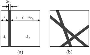
Figure 3: An adversary captures all nodes in the shaded region.

Since all $n$ nodes are uniformly distributed in the whole network region $\mathcal{A}$ with area $1$ ($\mathcal{A}$ is a unit torus or a unit square), then $\widetilde{N}$ (the number of nodes in the region $\widetilde{\mathcal{A}}$) follows a binomial distribution with parameter $n$ as the number of trials, and parameter $|\widetilde{\mathcal{A}}|$ as the success probability in each trial. For any $\nu_{n}>0$, we use Hoeffding’s inequality to have

$$\mathbb{P}[(|\widetilde{\mathcal{A}}|-\nu_{n})n\leq\widetilde{N}\leq(|\widetilde{\mathcal{A}}|+\nu_{n})n]\geq 1-2e^{-2{\nu_{n}}^{2}n}.$$ (60)

Setting $\nu_{n}=n^{-\frac{1}{3}}$, we have $2e^{-2{\nu_{n}}^{2}n}=o(1)$. Then

$$\mathbb{P}[(|\widetilde{\mathcal{A}}|-\nu_{n})n\leq\widetilde{N}\leq(|\widetilde{\mathcal{A}}|+\nu_{n})n]\geq 1-o(1).$$ (61)

Then we have

• if $|\widetilde{\mathcal{A}}|=o(1)$, then $\widetilde{N}\leq(|\widetilde{\mathcal{A}}|+\nu_{n})n=o(n)$ holds with high probability.

• if $|\widetilde{\mathcal{A}}|=\Theta(1)$, it holds with high probability that $(|\widetilde{\mathcal{A}}|-\nu_{n})n\leq\widetilde{N}\leq(|\widetilde{\mathcal{A}}|+\nu_{n})n$. From $|\widetilde{\mathcal{A}}|=\Theta(1)$ and $\nu_{n}=n^{-\frac{1}{3}}$, both $(|\widetilde{\mathcal{A}}|-\nu_{n})n$ and $(|\widetilde{\mathcal{A}}|+\nu_{n})n$ are $\Theta(n)$. Therefore, $\widetilde{N}=\Theta(n)$ follows with high probability.

Therefore, the results ❶ and ❷ above are proved. Returning to Figure 3-(a), as explained before, in view of $|\mathcal{A}_{0}|=o(1)$, $|\mathcal{A}_{1}|=\Theta(1)$ and $|\mathcal{A}_{2}|=\Theta(1)$, we obtain the following: with $N_{i}$ denoting the number of nodes in region $\mathcal{A}_{i}$ for each $i=0,1,2$, we have $N_{0}=o(n)$ with high probability, $N_{1}=\Theta(n)$ with high probability, and $N_{2}=\Theta(n)$ with high probability. Then $\big{\{}N_{0}=o(n)\big{\}}\hskip 2.0pt{\cap}\hskip 2.0pt\big{\{}N_{1}=\Theta(n)\big{\}}\hskip 2.0pt{\cap}\hskip 2.0pt\big{\{}N_{2}=\Theta(n)\big{\}}$ occurs with probability $1-o(1)$ by the union bound. Hence, $\big{\{}N_{0}=o(n)\big{\}}\hskip 2.0pt{\cap}\hskip 2.0pt\big{\{}N_{1}=\Theta(n)\big{\}}\hskip 2.0pt{\cap}\hskip 2.0pt\big{\{}N_{2}=\Theta(n)\big{\}}$ holds with high probability.

From Figure 3-(a), it is clear that any node in region $\mathcal{A}_{1}$ and any node in region $\mathcal{A}_{2}$ have a distance at least $2r_{n}$, so the node set in region $\mathcal{A}_{1}$ and the node set in region $\mathcal{A}_{2}$ have no edge in between. Hence, with high probability, an adversary that has captured $o(n)$ nodes in region $N_{0}$ partitions the network into two chunks, which both have linear sizes of sensors and are isolated from each other. Then the studied static secure sensor network with the $q$-composite scheme under the disk model on the unit torus or unit square is splittable. $\blacksquare$

Remarks:

• The adversary may split the network into multiple chunks instead of just two, as illustrated in Figure 3-(b).

• A future direction is to extended the result to more general topology (here we consider a torus or square).

VI-F Proof of Theorem 12

We will prove Theorem 12 by showing that under ${P_{n}}/{K_{n}}=\Omega(n)$, an adversary that has captured an arbitrary set of $o(n)$ sensors can only compromise $o(1)$ fraction of communication links in the rest of the network.

Suppose the adversary has captured some set of $m$ nodes. The choice of $m$ nodes depends on the adversary’s goal and also physical limitations (e.g., some sensors may be easier to be captured than others). Let $E_{\tau}$ be the event that the $m$ captured nodes have $\tau$ different keys in their key rings in total. It is clear that $K_{n}\leq\tau\leq\min\{mK_{n},P_{n}\}$. Recall that $p_{\textnormal{compromised}}$ is the fraction of compromised communications among non-captured nodes ($p_{\textnormal{compromised}}$ is also the probability that the secure link between two non-captured nodes is compromised). Conditioning on event $E_{\tau}$, let $p_{\textnormal{compromised}}(\tau)$ be the fraction of compromised communications among non-captured nodes (conditioning on event $E_{\tau}$, $p_{\textnormal{compromised}}(\tau)$ is also the probability that the secure link between two non-captured nodes is compromised). By the law of total probability, we have

$$p_{\textnormal{compromised}} =\textstyle{\sum_{\tau=K_{n}}^{\min\{mK_{n},P_{n}\}}\big{\{}\mathbb{P}[E_{\tau}]\cdot p_{\textnormal{compromised}}(\tau)\big{\}}}.$$ (62)

The adversary’s node capture strategy determines $\mathbb{P}[E_{\tau}]$. With $K_{n}\leq\tau\leq\min\{mK_{n},P_{n}\}$, it holds that $\sum_{K_{n}}^{\min\{mK_{n},P_{n}\}}\mathbb{P}[E_{\tau}]=1$. Clearly, as $\tau$ increases, $p_{\textnormal{compromised}}(\tau)$ increases (of course, if $\tau$ reaches $P_{n}$, $p_{\textnormal{compromised}}(\tau)$ becomes $1$ and can not increase anymore). With $K_{n}\leq\tau\leq\min\{mK_{n},P_{n}\}$, then $p_{\textnormal{compromised}}(\tau)$ achieves its maximum when $\tau=\min\{mK_{n},P_{n}\}$. Therefore, for an adversary that has captured any set of $m$ sensors, it is simple to derive from (62) that

$$p_{\textnormal{compromised}} \leq p_{\textnormal{compromised}}(\min\{mK_{n},P_{n}\}).$$ (63)

Under ${P_{n}}/{K_{n}}=\Omega(n)$ and $m=o(n)$, it holds that

$$mK_{n}=o(P_{n}).$$ (64)

Then we have $mK_{n}\leq P_{n}$ and thus $\min\{mK_{n},P_{n}\}=mK_{n}$ for all $n$ sufficiently large, which is used in (63) to derive

$$p_{\textnormal{compromised}} \leq p_{\textnormal{compromised}}(mK_{n}).$$ (65)

In addition, to maximize $p_{\textnormal{compromised}}$ as $p_{\textnormal{compromised}}(mK_{n})$, the adversary can capture some set of $m$ sensors which have $mK_{n}$ different keys in their key rings in total. Therefore, given (65), the proof of Theorem 12 is completed once we demonstrate $p_{\textnormal{compromised}}(mK_{n})=o(1)$.

By Yum and Lee [51], it follows that

$$\textstyle{p_{\textnormal{compromised}}(\tau)=\sum_{u=q}^{K_{n}}\bigg{[}\frac{\binom{\tau}{u}}{\binom{P_{n}}{u}}\cdot\frac{\rho_{u}}{p_{q}}\bigg{]}},$$ (66)

where the expressions of $\rho_{u}$ and $p_{q}$ are given in (22) and (23).

To compute $p_{\textnormal{compromised}}(mK_{n})$, we look at $p_{\textnormal{compromised}}(\tau)$ given in (66). Then we bound the term $\binom{\tau}{u}\Big{/}\binom{P_{n}}{u}$ in (66). With $q\leq u\leq K_{n}$, we obtain

$$\textstyle{\binom{\tau}{u}\big{/}\binom{P_{n}}{u}\leq\frac{\tau^{u}/(u!)}{{(P_{n}-u)}^{u}/(u!)}\leq\frac{\tau^{q}}{{(P_{n}-K_{n})}^{q}}},$$ (67)

which along with $\sum_{u=q}^{K_{n}}\rho_{u}=p_{q}$ is used in (66) to yield

$$p_{\textnormal{compromised}}(\tau)\leq\textstyle{\sum_{u=q}^{K_{n}}\big{[}\frac{\tau^{q}}{{(P_{n}-K_{n})}^{q}}\cdot\frac{\rho_{u}}{p_{q}}\big{]}=\frac{\tau^{q}}{{(P_{n}-K_{n})}^{q}}}.$$ (68)

Setting $\tau$ as $mK_{n}$, we have

$$p_{\textnormal{compromised}}(mK_{n})\leq\textstyle{\frac{(mK_{n})^{q}}{{(P_{n}-K_{n})}^{q}}}=o(1),$$ (69)

where the last step uses $mK_{n}=o(P_{n}-K_{n})$, which holds from (64). $\blacksquare$

VI-G Proof of Theorem 13

Note that different from the case of Theorem 12, in Theorem 13 here, we do not have $mK_{n}\leq P_{n}$ for all $n$ sufficiently large. Hence, we can have (63) only, instead of having (65).

When the adversary captures $m$ nodes randomly, $\mathbb{P}[E_{\tau}]$ is non-zero for all $\tau$ satisfying $K_{n}\leq\tau\leq\min\{mK_{n},P_{n}\}$. Under this random attack, the computation of $p_{\textnormal{compromised}}$ is not that straightforward. Yet, [17] presents an asymptotic expression of $p_{\textnormal{compromised}}$ as Lemma 12 below.

Lemma 12.

If the adversary captures $m$ nodes randomly with $m=o\big{(}\sqrt{\frac{P_{n}}{{K_{n}}^{2}}}\hskip 2.0pt\big{)}$, then $p_{\textnormal{compromised}}$ is asymptotically equivalent to $\big{(}\frac{mK_{n}}{P_{n}}\big{)}^{q}$ under $K_{n}=\omega(1)$ and $K_{n}=o\big{(}\sqrt{P_{n}}\big{)}$.

From Lemma 12, it holds that

$$p_{\textnormal{compromised}} \sim\textstyle{\big{(}\frac{mK_{n}}{P_{n}}\big{)}^{q}}.$$ (70)

Under $K_{n}=\omega(1)$ and $K_{n}=o\big{(}\sqrt{P_{n}}\big{)}$, as given in (18), we have $p_{q}\sim\frac{1}{q!}\cdot\frac{{K_{n}}^{2q}}{{P_{n}}^{q}}$, which with (70) above induces

$$\textstyle{\frac{p_{\textnormal{compromised}}}{p_{q}}\sim\big{(}\frac{mK_{n}}{P_{n}}\big{)}^{q}\cdot q!\cdot\frac{{P_{n}}^{q}}{{K_{n}}^{2q}}=q!\big{(}\frac{m}{K_{n}}\big{)}^{q}=f(q)},$$ (71)

where $f(q)$ is defined by

$$\textstyle{f(q)=q!\big{(}\frac{m}{K_{n}}\big{)}^{q}}.$$ (72)

We now analyze how $f(q)$ changes as $q$ varies, to understand the asymptotic behavior of $p_{\textnormal{compromised}}$. From (72), we compute $f(q+1)/f(q)$ through

$$\textstyle{\frac{f(q+1)}{f(q)}=\frac{m(q+1)}{K_{n}}}.$$ (73)

Then using (73) to analyze the monotonicity of $f(q)$, we finally establish Theorem 13.

VII Simulation Results

We now provide simulation results to confirm the theoretical findings. All plots in the paper are obtained from simulation. Specifically, in each plot, the data points are obtained by averaging over $500$ independent network samples.

VII-A Simulation Results for Connectivity

We present below simulation results of connectivity in secure sensor networks to confirm the theorems. Figure 4 depicts the probability that network $\textnormal{static-network}^{\textnormal{disk model}}_{\textnormal{unit torous}}$ is connected with $q=2$. We vary the key ring size $K$, and set $n=2000$, $P=5000$, and $r=0.2,0.3$. For each pair $(K,r)$, we generate $500$ independent samples of $\mathbb{G}_{q}(n,K,P,r,\mathcal{T})$ and record the count that the obtained graph has connectivity. Then we derive the empirical probabilities after dividing the counts by $500$. Similarly, in Figure 5, we plot the probability that network $\textnormal{static-network}^{\begin{subarray}{\textnormal{missing}}{\textnormal{disk model}}\\ \textnormal{unit square}\end{subarray}}_{\textnormal{unreliable links}}$ is connected after an adversary captures 10 random nodes, for $q=2$, $n=1000,900,800$, $P=5000$, $r=0.3$ and $t=0.9$. As illustrated in both figures, we observe the transitional behavior of connectivity. Moreover, for both Figure 4 and 5, substituting the parameter values into the corresponding theorems of this paper, we can confirm the correctness of the theorems.

Figure 6 presents a plot of the empirical probability that mobile network $\textnormal{mobile-network}^{\textnormal{disk model}}_{\textnormal{unit square}}$ is connected for at least $T$ consecutive time slots as a function of the key ring size with $q=2$, $n=1000$, $P=6000$, $r=0.25$ and $K=44,50,60$. We consider the i.i.d. mobility model, where each node independently picks a new location uniformly at random at the beginning of a time slot and stays at the location in the rest of the time slot. At each time slot, we check whether the network is connected. We generate $500$ independent samples and record the count that $\textnormal{mobile-network}^{\textnormal{disk model}}_{\textnormal{unit square}}$ is connected for at least $T$ consecutive time slots. Then we derive the empirical probabilities after dividing the counts by $500$. As illustrated in Figure 6, incrementing $K$ increases the probability that mobile network $\textnormal{mobile-network}^{\textnormal{disk model}}_{\textnormal{unit square}}$ is connected for at least $T$ consecutive time slots.

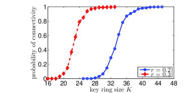
Figure 4: A plot of the empirical probability that network $\textnormal{static-network}^{\textnormal{disk model}}_{\textnormal{unit torous}}$ is connected as a function of the key ring size $K$ with $q=2$, $n=2000$, $P=5000$, and $r=0.2,0.3$.

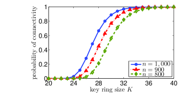
Figure 5: A plot of the empirical probability that network $\textnormal{static-network}^{\begin{subarray}{\textnormal{missing}}{\textnormal{disk model}}\\ \textnormal{unit square}\end{subarray}}_{\textnormal{unreliable links}}$ after the random capture of 10 nodes is connected as a function of the key ring size $K$ with $q=2$, $n=1000,900,800$, $P=5000$, $r=0.3$ and $t=0.9$.

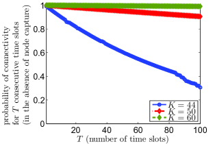
Figure 6: A plot of the empirical probability that mobile network $\textnormal{mobile-network}^{\textnormal{disk model}}_{\textnormal{unit square}}$ is connected for at least $T$ consecutive time slots as a function of the key ring size with $q=2$, $n=1000$, $P=6000$, $r=0.25$ and $K=44,50,60$.

VII-B Simulation Results for Unassailability

We provide simulation plots below for a comparison with the theoretical results above.

VII-B1 Varying $q$ with key ring size and key-setup prob. fixed

We first fix the key ring size and the key-setup probability, and vary $q$ to see how the probability $p_{\textnormal{compromised}}$ of link compromise changes.

Figure 7 depicts probability $p_{\textnormal{compromised}}$ with respect to $q$. We fix the key ring size at $K=40$, and the key-setup probability at $p_{q}=0.1$, and set the number $m$ of captured nodes as $15$ or $40$. As illustrated, for $m=15$, as $q$ increases, $p_{\textnormal{compromised}}$ first decreases and then increases; and for $m=40$, as $q$ increases, $p_{\textnormal{compromised}}$ always increases. These are in agreement with the analytical results. In particular, for $K=40$ and $m=15$, given $\frac{K}{m}=\frac{40}{15}\approx 2.67$ and Theorem 13, $p_{\textnormal{compromised}}$ takes its minimum at $q=2$, in accordance with the fact that in Figure 7, $p_{\textnormal{compromised}}$ for $m=15$ achieves its minimum at $q=2$. For $K=40$ and $m=40$, both both theoretical and experimental results show that $p_{\textnormal{compromised}}$ takes the minimum at $q=2$.

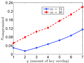
Figure 7: A plot of probability $p_{\textnormal{compromised}}$ of link compromise with respect to $q$, under $K=40$, $p_{q}=0.1$ and $m=15,40$. To ensure a fixed $p_{q}$, the key pool size $P$ needs to decrease as $q$ increases.

In Figure 8, we plot the relation between $q$ and the number $m$ of sensors that the adversary needs to capture to compromise a link between two non-captured nodes with probability $p_{\textnormal{compromised}}$. We also fix the key ring size at $K=40$, and the key-setup probability at $p_{q}=0.1$, and set $p_{\textnormal{compromised}}$ as $0.03$ or $0.1$. The curves on how $m$ changes with respect to $q$ also confirm the analytical results as explained below. As mentioned, for small $m$, as $q$ increases, $p_{\textnormal{compromised}}$ asymptotically first decreases and then increases. Hence, if we fix a small $p_{\textnormal{compromised}}$, as $q$ increases, the required $m$ should first increase and then decrease. This clearly is validated by the curve of $p_{\textnormal{compromised}}=0.03$ in Figure 8. Similarly, the theoretical result shows that for large $m$, as $q$ increases, $p_{\textnormal{compromised}}$ asymptotically always increases. Thus, if we fix a large $p_{\textnormal{compromised}}$, as $q$ increases, the required $m$ should always decrease. This is validated by the curve of $p_{\textnormal{compromised}}=0.1$ in Figure 8.

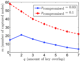
Figure 8: A plot under varying $q$ for the number $m$ of nodes that the adversary has to capture to compromise a link between two non-captured nodes with probability $p_{\textnormal{compromised}}$. The parameters are $K=40$, $p_{q}=0.1$ and $p_{\textnormal{compromised}}=0.03,0.1$. To fix $p_{q}$, the key pool size $P$ decreases as $q$ increases.

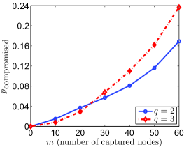
Figure 9: A plot of probability $p_{\textnormal{compromised}}$ of link compromise with respect to $m$, under $K=50$, $P=10000$ and $q=2,3$. Note that the key-setup probability here is different for different $q$.

VII-B2 Varying $m$ with key ring size and key pool size fixed

We now fix both the key ring size and the key pool size, and vary $m$ (the number of nodes captured by the adversary) to see how the probability $p_{\textnormal{compromised}}$ of link compromise changes with respect to $m$.

Figure 9 depicts probability $p_{\textnormal{compromised}}$ with respect to $m$. We fix the key ring size at $K=50$, and the key pool size at $P=10000$, and set $q$ (the required amount of key overlap) as $2$ or $3$. Clearly, for each $q$, we observe that $p_{\textnormal{compromised}}$ increases as $m$ increases. In addition, as we see, for very small $m$, probability $p_{\textnormal{compromised}}$ under $q=2$ is larger than that under $q=3$. We explain below that this confirms the theoretical result. By analysis, for small $m$ and small $q$, as $q$ increases, $p_{\textnormal{compromised}}$ asymptotically decreases. Therefore, for small $m$, $p_{\textnormal{compromised}}$ under $q=2$ is asymptotically larger than that under $q=3$, which is in agreement with Figure 9. By analysis, for large $m$, as $q$ increases, $p_{\textnormal{compromised}}$ asymptotically increases. This is validated since we see in Figure 9 that for large $m$, $p_{\textnormal{compromised}}$ under $q=2$ is small than that under $q=3$.

VIII Conclusion

In wireless sensor networks, the $q$-composite key predistribution scheme is a widely studied mechanism to secure communications. Despite considerable studies on secure sensor networks under the $q$-composite scheme, most of them ignore one or more than one of the following aspects: node-capture attacks, sensor mobility, physical transmission constraints, the boundary effect of network fields, and link unreliability, whereas we consider all of them in this paper and present conditions to ensure secure connectivity. Moreover, few researches on the $q$-composite scheme formally analyze the scheme’s resilience to arbitrary node-capture attacks considered in this paper, where the adversary can capture an arbitrary set of sensors. In the presence of arbitrary node-capture attacks, we derive conditions to ensure unassailability and unsplittability in secure sensor networks under the $q$-composite scheme. This paper presents a rigorous and comprehensive analysis to provide useful guidelines for connectivity and resilience design of secure sensor networks.

References

- [1] H. Chan, A. Perrig, and D. Song, “Random key predistribution schemes for sensor networks,” in IEEE Symposium on Security and Privacy, May 2003, pp. 197–213.
- [2] L. Eschenauer and V. Gligor, “A key-management scheme for distributed sensor networks,” in ACM Conference on Computer and Communications Security (CCS), 2002, pp. 41–47.
- [3] W. Du, J. Deng, Y. S. Han, P. K. Varshney, J. Katz, and A. Khalili, “A pairwise key predistribution scheme for wireless sensor networks,” ACM Transactions on Information and System Security (TISSEC), vol. 8, no. 2, pp. 228–258, 2005.
- [4] O. Yağan and A. M. Makowski, “Zero–one laws for connectivity in random key graphs,” IEEE Transactions on Information Theory, vol. 58, no. 5, pp. 2983–2999, May 2012.
- [5] O. Yağan, “Performance of the Eschenauer–Gligor key distribution scheme under an on/off channel,” IEEE Transactions on Information Theory, vol. 58, no. 6, pp. 3821–3835, June 2012.
- [6] R. Di Pietro, L. V. Mancini, A. Mei, A. Panconesi, and J. Radhakrishnan, “Connectivity properties of secure wireless sensor networks,” in ACM Workshop on Security of Ad hoc and Sensor Networks, 2004, pp. 53–58.
- [7] M. Bloznelis, J. Jaworski, and K. Rybarczyk, “Component evolution in a secure wireless sensor network,” Networks, vol. 53, pp. 19–26, January 2009.
- [8] J. Zhao, “Topological properties of wireless sensor networks under the -composite key predistribution scheme with unreliable links,” IEEE/ACM Transactions on Networking, vol. 25, no. 3, pp. 1789–1802, June 2017.
- [9] M. Bloznelis, “Degree and clustering coefficient in sparse random intersection graphs,” The Annals of Applied Probability, vol. 23, no. 3, pp. 1254–1289, 2013.
- [10] M. Bloznelis and T. Łuczak, “Perfect matchings in random intersection graphs,” Acta Mathematica Hungarica, vol. 138, no. 1-2, pp. 15–33, 2013.
- [11] F. Gandino, R. Ferrero, and M. Rebaudengo, “A key distribution scheme for mobile wireless sensor networks: --composite,” IEEE Transactions on Information Forensics and Security, vol. 12, no. 1, pp. 34–47, Jan 2017.
- [12] D. Liu, P. Ning, and R. Li, “Establishing pairwise keys in distributed sensor networks,” ACM Transactions on Information and System Security (TISSEC), vol. 8, no. 1, pp. 41–77, 2005.
- [13] X. Cha, W. Ni, K. Zheng, R. P. Liu, and X. Niu, “Collaborative authentication in decentralized dense mobile networks with key predistribution,” IEEE Transactions on Information Forensics and Security, vol. 12, no. 10, pp. 2261–2275, October 2017.
- [14] J. Zhao, O. Yağan, and V. Gligor, “Connectivity in secure wireless sensor networks under transmission constraints,” in Allerton Conference on Communication, Control, and Computing, 2014, pp. 1294–1301.
- [15] R. Di Pietro, L. V. Mancini, A. Mei, A. Panconesi, and J. Radhakrishnan, “Sensor networks that are provably resilient,” in International Conference on Security and Privacy in Communication Networks (SECURECOMM), 2006, pp. 1–10.
- [16] R. Di Pietro, L. V. Mancini, A. Mei, A. Panconesi, and J. Radhakrishnan, “Redoubtable sensor networks,” ACM Transactions on Information and System Security (TISSEC), vol. 11, no. 3, pp. 13:1–13:22, 2008.
- [17] J. Zhao, “On resilience and connectivity of secure wireless sensor networks under node capture attacks,” IEEE Transactions on Information Forensics and Security, vol. 12, no. 3, pp. 557–571, March 2017.
- [18] J. Zhao, “On the resilience to node capture attacks of secure wireless sensor networks,” in Allerton Conference on Communication, Control, and Computing (Allerton), 2015, pp. 887–893.
- [19] A. Mei, A. Panconesi, and J. Radhakrishnan, “Unassailable sensor networks,” in International Conference on Security and Privacy in Communication Networks (SECURECOMM), 2008, pp. 26:1–26:10.
- [20] O. Yağan and A. M. Makowski, “Wireless sensor networks under the random pairwise key predistribution scheme: Can resiliency be achieved with small key rings?” IEEE/ACM Transactions on Networking, vol. 24, no. 6, pp. 3383–3396, December 2016.
- [21] A. Alarifi and W. Du, “Diversify sensor nodes to improve resilience against node compromise,” in ACM Workshop on Security of Ad Hoc and Sensor Networks (SASN), 2006, pp. 101–112.
- [22] H. Yang, F. Ye, Y. Yuan, S. Lu, and W. Arbaugh, “Toward resilient security in wireless sensor networks,” in ACM International Symposium on Mobile Ad Hoc Networking and Computing (MobiHoc), 2005, pp. 34–45.
- [23] T. M. Vu, R. Safavi-Naini, and C. Williamson, “Securing wireless sensor networks against large-scale node capture attacks,” in ACM Symposium on Information, Computer and Communications Security (AsiaCCS), 2010, pp. 112–123.
- [24] M. Conti, R. Di Pietro, L. V. Mancini, and A. Mei, “Emergent properties: Detection of the node-capture attack in mobile wireless sensor networks,” in Proc. ACM WiSec, 2008, pp. 214–219.
- [25] T. Bonaci, L. Bushnell, and R. Poovendran, “Node capture attacks in wireless sensor networks: A system theoretic approach,” in IEEE Conference on Decision and Control (CDC), 2010, pp. 6765–6772.
- [26] P. Tague and R. Poovendran, “Modeling node capture attacks in wireless sensor networks,” in Allerton Conference on Communication, Control, and Computing, 2008, pp. 1221–1224.
- [27] B. Krishnan, A. Ganesh, and D. Manjunath, “On connectivity thresholds in superposition of random key graphs on random geometric graphs,” in IEEE International Symposium on Information Theory (ISIT), 2013, pp. 2389–2393.
- [28] K. Krzywdziński and K. Rybarczyk, “Geometric graphs with randomly deleted edges — connectivity and routing protocols,” Mathematical Foundations of Computer Science, vol. 6907, pp. 544–555, 2011.
- [29] M. Bloznelis and K. Rybarczyk, “-connectivity of uniform -intersection graphs,” Discrete Mathematics, vol. 333, pp. 94–100, 2014.
- [30] J. Zhao, O. Yağan, and V. Gligor, “On -connectivity and minimum vertex degree in random -intersection graphs,” in ACM-SIAM Meeting on Analytic Algorithmics and Combinatorics (ANALCO), 2015, pp. 1–15.
- [31] J. Zhao, O. Yağan, and V. Gligor, “-Connectivity in random key graphs with unreliable links,” IEEE Transactions on Information Theory, vol. 61, no. 7, pp. 3810–3836, July 2015.
- [32] L. Fu, X. Wang, and P. Kumar, “Are we connected? Optimal determination of source–destination connectivity in random networks,” IEEE/ACM Transactions on Networking (TON), vol. 25, no. 2, pp. 751–764, 2017.
- [33] F. Yavuz, J. Zhao, O. Yağan, and V. Gligor, “Toward -connectivity of the random graph induced by a pairwise key predistribution scheme with unreliable links,” IEEE Transactions on Information Theory, vol. 61, no. 11, pp. 6251–6271, 2015.
- [34] F. Yavuz, J. Zhao, O. Yağan, and V. Gligor, “-connectivity in random -out graphs intersecting erdős-rényi graphs,” IEEE Transactions on Information Theory, vol. 63, no. 3, pp. 1677–1692, 2017.
- [35] O. Yağan and A. M. Makowski, “Modeling the pairwise key predistribution scheme in the presence of unreliable links,” IEEE Transactions on Information Theory, vol. 59, no. 3, pp. 1740–1760, 2013.
- [36] J. Zhao, “Analyzing resilience of interest-based social networks against node and link failures,” IEEE Transactions on Signal and Information Processing over Networks, vol. 3, no. 2, pp. 252–267, June 2017.
- [37] P. Gupta and P. R. Kumar, “Critical power for asymptotic connectivity in wireless networks,” in IEEE Conference on Decision and Control (CDC), 1998, pp. 547–566.
- [38] X. Liu, J. Zhang, L. Liu, W. Wu, X. Tian, X. Wang, W. Zhang, and J. Xu, “Network connectivity with inhomogeneous correlated mobility,” IEEE Transactions on Wireless Communications, vol. 15, no. 6, pp. 4307–4320, 2016.
- [39] M. Tomasini, F. Zambonelli, A. Brayner, and R. Menezes, “Evaluating the performance of social networks of sensors under different mobility models,” in International Conference on Social Computing (SocialCom). IEEE, 2013, pp. 397–402.
- [40] J. Xie, Y. Wan, J. H. Kim, S. Fu, and K. Namuduri, “A survey and analysis of mobility models for airborne networks,” IEEE Communications Surveys & Tutorials, vol. 16, no. 3, pp. 1221–1238, 2014.
- [41] R. J. La and E. Seo, “Network connectivity with a family of group mobility models,” IEEE Transactions on Mobile Computing, vol. 11, no. 3, pp. 504–517, 2012.
- [42] X. Liu, K. Zheng, J. Zhao, X.-Y. Liu, X. Wang, and X. Di, “Information-centric networks with correlated mobility,” IEEE Transactions on Vehicular Technology, vol. 66, no. 5, pp. 4256–4270, 2017.
- [43] J. Zhao, O. Yağan, and V. Gligor, “On topological properties of wireless sensor networks under the -composite key predistribution scheme with on/off channels,” in IEEE Int. Symp. Inf. Theory (ISIT), 2014, pp. 1131–1135.
- [44] K. Rybarczyk, “Sharp threshold functions for the random intersection graph via a coupling method,” The Electronic Journal of Combinatorics, vol. 18, pp. 36–47, 2011.
- [45] J. Zhao, O. Yağan, and V. Gligor, “On connectivity and robustness in random intersection graphs,” IEEE Transactions on Automatic Control, vol. 62, no. 5, pp. 2121–2136, 2017.
- [46] K. Rybarczyk, “The coupling method for inhomogeneous random intersection graphs.” The Electronic Journal of Combinatorics, vol. 24, no. 2, pp. P2–10, 2017.
- [47] J. Zhao, “Transitional behavior of -composite random key graphs with applications to networked control,” IEEE Transactions on Control of Network Systems, 2017.
- [48] P. Erdős and A. Rényi, “On random graphs, I,” Publicationes Mathematicae (Debrecen), vol. 6, pp. 290–297, 1959.
- [49] M. Bloznelis, J. Jaworski, and V. Kurauskas, “Assortativity and clustering of sparse random intersection graphs,” The Electronic Journal of Probability, vol. 18, no. 38, pp. 1–24, 2013.
- [50] M. D. Penrose et al., “Connectivity of soft random geometric graphs,” The Annals of Applied Probability, vol. 26, no. 2, pp. 986–1028, 2016.
- [51] D. H. Yum and P. J. Lee, “Exact formulae for resilience in random key predistribution schemes,” IEEE Transactions on Wireless Communications, vol. 11, no. 5, pp. 1638–1642, 2012.