Jacobi-type algorithm for low rank orthogonal approximation of symmetric tensors and its convergence analysis111This work was supported in part by the National Natural Science Foundation of China (No. 11601371, 11701327) and the ANR (Agence Nationale de Recherche) under grant LeaFleT (ANR-19-CE23-0021).

Jianze Li222Shenzhen Research Institute of Big Data, The Chinese University of Hong Kong, Shenzhen, China (lijianze@gmail.com), Konstantin Usevich333Université de Lorraine, CNRS, CRAN, Nancy, France (konstantin.usevich@univ-lorraine.fr), and Pierre Comon444Univ. Grenoble Alpes, CNRS, Grenoble INP, GIPSA-Lab, France (pierre.comon@gipsa-lab.fr)

Abstract: In this paper, we propose a Jacobi-type algorithm to solve the low rank orthogonal approximation problem of symmetric tensors. This algorithm includes as a special case the well-known Jacobi CoM2 algorithm for the approximate orthogonal diagonalization problem of symmetric tensors. We study the global convergence of this algorithm under a gradient based ordering for a special case: the best rank-2 orthogonal approximation of 3rd order symmetric tensors, and prove that an accumulation point is the unique limit point under some conditions. We also propose a proximal variant of this algorithm in general case, and prove its global convergence without any further condition. Numerical experiments are presented to show the efficiency of this algorithm.


Keywords: Jacobi-type algorithm; low rank orthogonal approximation; symmetric tensors; weak convergence; global convergence
Mathematics Subject Classification: 15A69, 15A23, 49M30, 65F99, 26E05

1 Introduction

As the higher order analogue of vectors and matrices, in the last two decades, tensors have been attracting more and more attentions from various fields, including signal processing, numerical linear algebra and machine learning [6, 10, 12, 21, 30, 2]. One reason is that more and more real data are naturally represented in tensor form, e.g. hyperspectral images, fMRI data, or social networks. The other reason is that, compared with the matrix case, tensor based techniques can capture higher order and more complicated relationships, e.g. Independent Component Analysis (ICA) based on the cumulant tensor [8], and multilinear subspace learning methods [25].

Low rank approximation of higher order tensors is a very important problem and has been applied in various areas [12, 14, 31]. However, it is much more difficult than the matrix case, since it is ill-posed for many ranks, and this ill-posedness is not rare for 3rd order tensors [17].

Notation. Let n1××nd=𝖽𝖾𝖿n1ndsuperscript𝖽𝖾𝖿superscriptsubscript𝑛1subscript𝑛𝑑tensor-productsuperscriptsubscript𝑛1superscriptsubscript𝑛𝑑\mathbb{R}^{n_{1}\times\cdots\times n_{d}}\stackrel{{\scriptstyle\sf def}}{{=}}\mathbb{R}^{n_{1}}\otimes\cdots\otimes\mathbb{R}^{n_{d}} be the space of d𝑑d-th order real tensors and symm(n××n)n××nsymmsuperscript𝑛𝑛superscript𝑛𝑛\text{symm}(\mathbb{R}^{n\times\cdots\times n})\subset\mathbb{R}^{n\times\cdots\times n} be the set of symmetric ones [11, 27], whose entries do not change under any permutation of indices. The identity matrix of size n𝑛n is denoted by 𝑰nsubscript𝑰𝑛\boldsymbol{I}_{n}. Let St(p,n)n×pSt𝑝𝑛superscript𝑛𝑝\text{St}(p,n)\subset\mathbb{R}^{n\times p} be the Stiefel manifold with 1pn1𝑝𝑛1\leq p\leq n. Let 𝒪nn×nsubscript𝒪𝑛superscript𝑛𝑛\mathscr{O}_{n}\subset\mathbb{R}^{n\times n} be the orthogonal group, i.e. 𝒪n=St(n,n)subscript𝒪𝑛St𝑛𝑛\mathscr{O}_{n}=\text{St}(n,n). Let 𝒮𝒪nn×n𝒮subscript𝒪𝑛superscript𝑛𝑛\mathscr{SO}_{n}\subset\mathbb{R}^{n\times n} be the special orthogonal group, i.e. the set of orthogonal matrices with determinant 1. We denote by \|\cdot\| the Frobenius norm of a tensor or a matrix, or the Euclidean norm of a vector. Tensor arrays, matrices, and vectors, will be respectively denoted by bold calligraphic letters, e.g. 𝓐𝓐\boldsymbol{\mathcal{A}}, with bold uppercase letters, e.g. 𝑴𝑴\boldsymbol{M}, and with bold lowercase letters, e.g. 𝒖𝒖\boldsymbol{u}; corresponding entries will be denoted by 𝒜ijksubscript𝒜𝑖𝑗𝑘\mathcal{A}_{ijk}, Mijsubscript𝑀𝑖𝑗M_{ij}, and uisubscript𝑢𝑖u_{i}. Operator psubscript𝑝\mathop{\bullet_{p}} denotes contraction on the p𝑝pth index of a tensor; when contracted with a matrix, it is understood that summation is always performed on the second index of the matrix. For instance, (𝓐1𝑴)ijk=𝒜jkMisubscript𝓐subscript1𝑴𝑖𝑗𝑘subscriptsubscript𝒜𝑗𝑘subscript𝑀𝑖(\boldsymbol{\mathcal{A}}\mathop{\bullet_{1}}\boldsymbol{M})_{ijk}=\sum_{\ell}\mathcal{A}_{\ell jk}M_{i\ell}. We denote

𝓐(𝑴)=𝖽𝖾𝖿𝓐1𝑴𝖳2d𝑴𝖳superscript𝖽𝖾𝖿𝓐𝑴𝓐subscript1superscript𝑴𝖳subscript2subscript𝑑superscript𝑴𝖳\boldsymbol{\mathcal{A}}(\boldsymbol{M})\stackrel{{\scriptstyle\sf def}}{{=}}\boldsymbol{\mathcal{A}}\mathop{\bullet_{1}}\boldsymbol{M}^{{\sf T}}\mathop{\bullet_{2}}\cdots\mathop{\bullet_{d}}\boldsymbol{M}^{{\sf T}}

for convenience in this paper. For 𝓐n××n𝓐superscript𝑛𝑛\boldsymbol{\mathcal{A}}\in\mathbb{R}^{n\times\cdots\times n} and a fixed set of indices 1k1<k2<<kmn1subscript𝑘1subscript𝑘2subscript𝑘𝑚𝑛1\leq k_{1}<k_{2}<\cdots<k_{m}\leq n, we denote by 𝓐(k1,k2,,km)superscript𝓐subscript𝑘1subscript𝑘2subscript𝑘𝑚\boldsymbol{\mathcal{A}}^{(k_{1},k_{2},\cdots,k_{m})} the m𝑚m-dimensional d𝑑d-th order subtensor obtained from 𝓐𝓐\boldsymbol{\mathcal{A}} by allowing its indices to take values in {k1,k2,,km}subscript𝑘1subscript𝑘2subscript𝑘𝑚\{k_{1},k_{2},\cdots,k_{m}\} only.

Problem statement. Let 𝓐symm(n××n)𝓐symmsuperscript𝑛𝑛\boldsymbol{\mathcal{A}}\in\text{symm}(\mathbb{R}^{n\times\cdots\times n}) and 1pn1𝑝𝑛1\leq p\leq n. In this paper, we study the best rank-p𝑝p orthogonal approximation problem, which is to find

𝓒=𝖽𝖾𝖿k=1pσkukuk,superscript𝖽𝖾𝖿superscript𝓒superscriptsubscript𝑘1𝑝tensor-productsuperscriptsubscript𝜎𝑘superscriptsubscript𝑢𝑘superscriptsubscript𝑢𝑘\boldsymbol{\mathcal{C}}^{*}\stackrel{{\scriptstyle\sf def}}{{=}}\sum\limits_{k=1}^{p}\sigma_{k}^{*}u_{k}^{*}\otimes\cdots\otimes u_{k}^{*}, (1.1)

where

(σ1,,σp,u1,,up)=argmin[u1,,up]St(p,n)σk,1kp𝓐k=1pσkukuk.superscriptsubscript𝜎1subscriptsuperscript𝜎𝑝subscriptsuperscript𝑢1subscriptsuperscript𝑢𝑝subscriptargminsubscript𝑢1subscript𝑢𝑝St𝑝𝑛formulae-sequencesubscript𝜎𝑘1𝑘𝑝norm𝓐superscriptsubscript𝑘1𝑝tensor-productsubscript𝜎𝑘subscript𝑢𝑘subscript𝑢𝑘(\sigma_{1}^{*},\ldots,\sigma^{*}_{p},u^{*}_{1},\ldots,u^{*}_{p})=\mathop{\operator@font argmin}_{\begin{subarray}{c}[u_{1},\cdots,u_{p}]\in\text{St}(p,n)\\ \sigma_{k}\in\mathbb{R},1\leq k\leq p\end{subarray}}\|\boldsymbol{\mathcal{A}}-\sum_{k=1}^{p}\sigma_{k}u_{k}\otimes\cdots\otimes u_{k}\|. (1.2)

If p=1𝑝1p=1, then (1.2) is the best rank-1 approximation problem [16, 19, 22, 33, 13] of symmetric tensors, which is equivalent to the cubic spherical optimization problem [28, 34, 35]. If p=n𝑝𝑛p=n, by [5, Proposition 5.1] and [24, Proposition 5.2], we see that (1.2) is closely related to the approximate orthogonal diagonalization problem for 3rd and 4th order cumulant tensors, which is in the core of Independent Component Analysis (ICA) [7, 8, 9], and finds many applications [12].

To our knowledge, the orthogonal tensor decomposition was first tackled in [7], but appeared more formally in [20], in which many examples were presented to illustrate the difficulties of this type of decomposition. As shown in [5], the minimum in problem (1.2) exists, and the low rank orthogonal approximation of tensors (LROAT) algorithm and symmetric LROAT (SLROAT) were developed to solve this problem based on the polar decomposition. In the special case p=1𝑝1p=1, the two algorithms boil down to the higher order power method (HOPM) and symmetric HOPM (SHOPM) algorithm [16, 19, 33]. More recently, also based on the polar decomposition, a similar algorithm was developed in [26] to solve problem (1.2), and this algorithm was applied to the image reconstruction task.

Contribution. The main contributions of this paper can be summarized as follows:

  • \bullet

    We propose a Jacobi-type algorithm for solving problem (1.2). This algorithm is exactly the well-known Jacobi CoM2 algorithm [12] when p=n𝑝𝑛p=n, and the same as the Jacobi-type algorithm for Tucker approximation proposed in [18] when p=1𝑝1p=1.

  • \bullet

    Under the gradient based ordering defined in [18, 23, 32], we prove the global convergence555the iterations converge to a unique limit point for any starting point. of this algorithm for 3rd order tensors of rank p=2𝑝2p=2 under some conditions.

  • \bullet

    We propose a proximal variant of this Jacobi-type algorithm, and prove its global convergence without any further condition.

Organization. The paper is organized as follows. In Section 2, we show that two optimization problems on Riemannian manifold St(p,n)St𝑝𝑛\text{St}(p,n) and orthogonal group 𝒪nsubscript𝒪𝑛\mathscr{O}_{n} are both equivalent to problem (1.2), and then calculate their Riemannian gradients. In Section 3, we propose a Jacobi-type algorithm to solve problem (1.2). This algorithm includes the well-known Jacobi CoM2 algorithm as a special case. In Section 4, we study the global convergence of this algorithm under the gradient based ordering for the 3rd order tensor and p=2𝑝2p=2 case. In Section 5, a proximal variant of this algorithm is proposed, and its global convergence is established. In Section 6, we report some numerical experiments showing the efficiency of this algorithm.

2 Geometric properties

2.1 Equivalent problems

Let 𝓐symm(n××n)𝓐symmsuperscript𝑛𝑛\boldsymbol{\mathcal{A}}\in\text{symm}(\mathbb{R}^{n\times\cdots\times n}) and 1pn1𝑝𝑛1\leq p\leq n. Let 𝑿St(p,n)𝑿St𝑝𝑛\boldsymbol{X}\in\text{St}(p,n) and 𝓦~=𝓐(𝑿).~𝓦𝓐𝑿\widetilde{\boldsymbol{\mathcal{W}}}=\boldsymbol{\mathcal{A}}(\boldsymbol{X}). One problem equivalent to (1.2) is to find

𝑿=argmax𝑿St(p,n)f~(𝑿),subscript𝑿subscript𝑿St𝑝𝑛~𝑓𝑿\boldsymbol{X}_{*}=\operatorname*{\arg\!\max}_{\boldsymbol{X}\in\text{St}(p,n)}\tilde{f}(\boldsymbol{X}), (2.1)

where

f~(𝑿)=𝖽𝖾𝖿i=1p𝒲~ii2.superscript𝖽𝖾𝖿~𝑓𝑿superscriptsubscript𝑖1𝑝subscriptsuperscript~𝒲2𝑖𝑖\tilde{f}(\boldsymbol{X})\stackrel{{\scriptstyle\sf def}}{{=}}\sum\limits_{i=1}^{p}\widetilde{\mathcal{W}}^{2}_{i\cdots i}. (2.2)
Lemma 2.1.

([5, Proposition 5.1]) Let 𝓒superscript𝓒\boldsymbol{\mathcal{C}}^{*} be as in (1.2). Then

𝓐𝓒,ukuk=0andσk=𝓐,ukuk𝓐superscript𝓒tensor-productsuperscriptsubscript𝑢𝑘superscriptsubscript𝑢𝑘0andsuperscriptsubscript𝜎𝑘𝓐tensor-productsuperscriptsubscript𝑢𝑘superscriptsubscript𝑢𝑘\langle\boldsymbol{\mathcal{A}}-\boldsymbol{\mathcal{C}}^{*},u_{k}^{*}\otimes\cdots\otimes u_{k}^{*}\rangle=0\ \ \text{and}\ \ \sigma_{k}^{*}=\langle\boldsymbol{\mathcal{A}},u_{k}^{*}\otimes\cdots\otimes u_{k}^{*}\rangle

for 1kp1𝑘𝑝1\leq k\leq p. Moreover, it holds that

𝓐𝓒2=𝓐2𝓒2=𝓐2k=1p(σk)2.superscriptnorm𝓐superscript𝓒2superscriptnorm𝓐2superscriptnormsuperscript𝓒2superscriptnorm𝓐2superscriptsubscript𝑘1𝑝superscriptsuperscriptsubscript𝜎𝑘2\|\boldsymbol{\mathcal{A}}-\boldsymbol{\mathcal{C}}^{*}\|^{2}=\|\boldsymbol{\mathcal{A}}\|^{2}-\|\boldsymbol{\mathcal{C}}^{*}\|^{2}=\|\boldsymbol{\mathcal{A}}\|^{2}-\sum\limits_{k=1}^{p}(\sigma_{k}^{*})^{2}. (2.3)
Remark 2.2.

(i) Let 𝓒superscript𝓒\boldsymbol{\mathcal{C}}^{*} be as in (1.2) and 𝑿subscript𝑿\boldsymbol{X}_{*} be as in (2.1). We see from (2.3) that

𝑿=[u1,,up]and𝓐𝓒2=𝓐2f~(𝑿).subscript𝑿superscriptsubscript𝑢1superscriptsubscript𝑢𝑝andsuperscriptnorm𝓐superscript𝓒2superscriptnorm𝓐2~𝑓subscript𝑿\boldsymbol{X}_{*}=[u_{1}^{*},\cdots,u_{p}^{*}]\ \ \text{and}\ \ \|\boldsymbol{\mathcal{A}}-\boldsymbol{\mathcal{C}}^{*}\|^{2}=\|\boldsymbol{\mathcal{A}}\|^{2}-\tilde{f}(\boldsymbol{X}_{*}).

In other words, to solve (1.2), it is enough for us to solve (2.1), which is an optimization problem on St(p,n)St𝑝𝑛\text{St}(p,n).
(ii) If p=1𝑝1p=1, then (2.1) is the cubic spherical optimization problem [28, 34, 35]. If p=n𝑝𝑛p=n, then (2.1) is the approximate orthogonal tensor diagonalization problem [8, 9, 12, 23].

Let 𝑸𝒪n𝑸subscript𝒪𝑛\boldsymbol{Q}\in\mathscr{O}_{n} and 𝓦=𝓐(𝑸)𝓦𝓐𝑸\boldsymbol{\mathcal{W}}=\boldsymbol{\mathcal{A}}(\boldsymbol{Q}). Another problem, equivalent to (2.1), is to find

𝑸=argmax𝑸𝒪nf(𝑸),subscript𝑸subscript𝑸subscript𝒪𝑛𝑓𝑸\boldsymbol{Q}_{*}=\operatorname*{\arg\!\max}_{\boldsymbol{Q}\in\mathscr{O}_{n}}f(\boldsymbol{Q}), (2.4)

where

f(𝑸)=𝖽𝖾𝖿i=1p𝒲ii2.superscript𝖽𝖾𝖿𝑓𝑸superscriptsubscript𝑖1𝑝subscriptsuperscript𝒲2𝑖𝑖f(\boldsymbol{Q})\stackrel{{\scriptstyle\sf def}}{{=}}\sum\limits_{i=1}^{p}\mathcal{W}^{2}_{i\cdots i}. (2.5)

In fact, if 𝑿St(p,n)𝑿St𝑝𝑛\boldsymbol{X}\in\text{St}(p,n) and 𝑸=[𝑿,𝒀]𝒪n𝑸𝑿𝒀subscript𝒪𝑛\boldsymbol{Q}=[\boldsymbol{X},\boldsymbol{Y}]\in\mathscr{O}_{n}, then 𝒲i1id=𝒲~i1idsubscript𝒲subscript𝑖1subscript𝑖𝑑subscript~𝒲subscript𝑖1subscript𝑖𝑑\mathcal{W}_{i_{1}\cdots i_{d}}=\widetilde{\mathcal{W}}_{i_{1}\cdots i_{d}} for any 1i1,,idpformulae-sequence1subscript𝑖1subscript𝑖𝑑𝑝1\leq i_{1},\cdots,i_{d}\leq p. The equivalence between (2.1) and (2.4) follows from the fact that f(𝑸)=f~(𝑿)𝑓𝑸~𝑓𝑿f(\boldsymbol{Q})=\tilde{f}(\boldsymbol{X}).

Remark 2.3.

Let 𝓦symm(n×n×n)𝓦symmsuperscript𝑛𝑛𝑛\boldsymbol{\mathcal{W}}\in\text{symm}(\mathbb{R}^{n\times n\times n}) and 1pn1𝑝𝑛1\leq p\leq n. Let 𝓦~=𝓦(1,2,,p)~𝓦superscript𝓦12𝑝\widetilde{\boldsymbol{\mathcal{W}}}=\boldsymbol{\mathcal{W}}^{(1,2,\cdots,p)}. Then the objective used in [18, (3.1)] is the sum of squares of all the elements in 𝓦~~𝓦\widetilde{\boldsymbol{\mathcal{W}}}, while (2.5) is the sum of squares of the diagonal elements in 𝓦~~𝓦\widetilde{\boldsymbol{\mathcal{W}}}. They are the same if p=1𝑝1p=1.

2.2 Riemannian gradient

Definition 2.4.

Let 𝓐symm(n××n)𝓐symmsuperscript𝑛𝑛\boldsymbol{\mathcal{A}}\in\text{symm}(\mathbb{R}^{n\times\cdots\times n}) and 1i<jn1𝑖𝑗𝑛1\leq i<j\leq n. Define

σi,j(𝓐)=𝖽𝖾𝖿𝒜iii𝒜jii,di,j(𝓐)=𝖽𝖾𝖿σi,j(𝓐)σj,i(𝓐)=𝒜iii𝒜jii𝒜ijj𝒜jjj.formulae-sequencesuperscript𝖽𝖾𝖿subscript𝜎𝑖𝑗𝓐subscript𝒜𝑖𝑖𝑖subscript𝒜𝑗𝑖𝑖superscript𝖽𝖾𝖿subscript𝑑𝑖𝑗𝓐subscript𝜎𝑖𝑗𝓐subscript𝜎𝑗𝑖𝓐subscript𝒜𝑖𝑖𝑖subscript𝒜𝑗𝑖𝑖subscript𝒜𝑖𝑗𝑗subscript𝒜𝑗𝑗𝑗\displaystyle\sigma_{i,j}(\boldsymbol{\mathcal{A}})\stackrel{{\scriptstyle\sf def}}{{=}}\mathcal{A}_{ii\ldots i}\mathcal{A}_{ji\ldots i},\quad d_{i,j}(\boldsymbol{\mathcal{A}})\stackrel{{\scriptstyle\sf def}}{{=}}\sigma_{i,j}(\boldsymbol{\mathcal{A}})-\sigma_{j,i}(\boldsymbol{\mathcal{A}})=\mathcal{A}_{ii\ldots i}\mathcal{A}_{ji\ldots i}-\mathcal{A}_{ij\ldots j}\mathcal{A}_{jj\ldots j}.
Theorem 2.5.

The Riemannian gradient of (2.5) at 𝑸𝑸\boldsymbol{Q} is

gradf(𝑸)=𝑸Λ(𝑸),grad𝑓𝑸𝑸Λ𝑸\mathop{{\operator@font grad}}f(\boldsymbol{Q})=\boldsymbol{Q}\,\Lambda(\boldsymbol{Q}), (2.6)

where

Λ(𝑸)=𝖽𝖾𝖿d[0d1,2(𝓦)d1,p(𝓦)σ1,p+1(𝓦)σ1,n(𝓦)d1,2(𝓦)0d2,p(𝓦)σ2,p+1(𝓦)σ2,n(𝓦)d1,p(𝓦)d2,p(𝓦)0σp,p+1(𝓦)σp,n(𝓦)σ1,p+1(𝓦)σ2,p+1(𝓦)σp,p+1(𝓦)00σ1,n(𝓦)σ2,n(𝓦)σp,n(𝓦)00].superscript𝖽𝖾𝖿Λ𝑸𝑑delimited-[]0subscript𝑑12𝓦subscript𝑑1𝑝𝓦subscript𝜎1𝑝1𝓦subscript𝜎1𝑛𝓦missing-subexpressionsubscript𝑑12𝓦0subscript𝑑2𝑝𝓦subscript𝜎2𝑝1𝓦subscript𝜎2𝑛𝓦missing-subexpressionmissing-subexpressionsubscript𝑑1𝑝𝓦subscript𝑑2𝑝𝓦0subscript𝜎𝑝𝑝1𝓦subscript𝜎𝑝𝑛𝓦missing-subexpressionsubscript𝜎1𝑝1𝓦subscript𝜎2𝑝1𝓦subscript𝜎𝑝𝑝1𝓦00missing-subexpressionmissing-subexpressionsubscript𝜎1𝑛𝓦subscript𝜎2𝑛𝓦subscript𝜎𝑝𝑛𝓦00\displaystyle\Lambda(\boldsymbol{Q})\stackrel{{\scriptstyle\sf def}}{{=}}d\cdot\left[\begin{smallmatrix}0&-d_{1,2}(\boldsymbol{\mathcal{W}})&\ldots&-d_{1,p}(\boldsymbol{\mathcal{W}})&-\sigma_{1,p+1}(\boldsymbol{\mathcal{W}})&\cdots&-\sigma_{1,n}(\boldsymbol{\mathcal{W}})\\ \\ d_{1,2}(\boldsymbol{\mathcal{W}})&0&\ldots&-d_{2,p}(\boldsymbol{\mathcal{W}})&-\sigma_{2,p+1}(\boldsymbol{\mathcal{W}})&\cdots&-\sigma_{2,n}(\boldsymbol{\mathcal{W}})\\ \\ \ldots&\ldots&\ldots&\ldots&\cdots&\cdots&\cdots\\ \\ d_{1,p}(\boldsymbol{\mathcal{W}})&d_{2,p}(\boldsymbol{\mathcal{W}})&\ldots&0&-\sigma_{p,p+1}(\boldsymbol{\mathcal{W}})&\cdots&-\sigma_{p,n}(\boldsymbol{\mathcal{W}})\\ \\ \sigma_{1,p+1}(\boldsymbol{\mathcal{W}})&\sigma_{2,p+1}(\boldsymbol{\mathcal{W}})&\cdots&\sigma_{p,p+1}(\boldsymbol{\mathcal{W}})&0&\cdots&0\\ \\ \ldots&\ldots&\ldots&\ldots&\ldots&\cdots&\ldots\\ \\ \sigma_{1,n}(\boldsymbol{\mathcal{W}})&\sigma_{2,n}(\boldsymbol{\mathcal{W}})&\ldots&\sigma_{p,n}(\boldsymbol{\mathcal{W}})&0&\cdots&0\end{smallmatrix}\right]. (2.7)
Proof.

Note that

f(𝑸)=j=1p𝒲jjj2=j=1p(i1,i2,,id𝒜i1,i2,,idQi1,jQi2,jQid,j)2.𝑓𝑸superscriptsubscript𝑗1𝑝subscriptsuperscript𝒲2𝑗𝑗𝑗superscriptsubscript𝑗1𝑝superscriptsubscriptsubscript𝑖1subscript𝑖2subscript𝑖𝑑subscript𝒜subscript𝑖1subscript𝑖2subscript𝑖𝑑subscript𝑄subscript𝑖1𝑗subscript𝑄subscript𝑖2𝑗subscript𝑄subscript𝑖𝑑𝑗2f(\boldsymbol{Q})=\sum\limits_{j=1}^{p}\mathcal{W}^{2}_{jj\ldots j}=\sum\limits_{j=1}^{p}(\sum\limits_{i_{1},i_{2},\ldots,i_{d}}\mathcal{A}_{i_{1},i_{2},\ldots,i_{d}}Q_{i_{1},j}Q_{i_{2},j}\ldots Q_{i_{d},j})^{2}.

Let 𝓥=𝓐2𝑸𝖳d𝑸𝖳𝓥𝓐subscript2superscript𝑸𝖳subscript𝑑superscript𝑸𝖳\boldsymbol{\mathcal{V}}=\boldsymbol{\mathcal{A}}\mathop{\bullet_{2}}\boldsymbol{Q}^{{\sf T}}\cdots\mathop{\bullet_{d}}\boldsymbol{Q}^{{\sf T}}. Fix 1in1𝑖𝑛1\leq i\leq n and 1jp1𝑗𝑝1\leq j\leq p. Then

fQi,j=2d𝒲jjj𝒱ijj𝑓subscript𝑄𝑖𝑗2𝑑subscript𝒲𝑗𝑗𝑗subscript𝒱𝑖𝑗𝑗\displaystyle\frac{\partial f}{\partial{Q}_{i,j}}=2d\mathcal{W}_{jj\ldots j}\mathcal{V}_{ij\ldots j}

by methods similar to [23, Section 4.1]. Note that 𝓦=𝓥1𝑸𝖳𝓦𝓥subscript1superscript𝑸𝖳\boldsymbol{\mathcal{W}}=\boldsymbol{\mathcal{V}}\mathop{\bullet_{1}}\boldsymbol{Q}^{{\sf T}}. We get the Euclidean gradient of (2.5) at 𝑸𝑸\boldsymbol{Q} as follows:

f(𝑸)=2d𝑸[𝒲111𝒲122𝒲1pp00𝒲211𝒲222𝒲2pp00𝒲n11𝒲n22𝒲npp00][𝒲110000𝒲pp0000].𝑓𝑸2𝑑𝑸matrixsubscript𝒲111subscript𝒲122subscript𝒲1𝑝𝑝00subscript𝒲211subscript𝒲222subscript𝒲2𝑝𝑝00missing-subexpressionsubscript𝒲𝑛11subscript𝒲𝑛22subscript𝒲𝑛𝑝𝑝00matrixsubscript𝒲110000subscript𝒲𝑝𝑝0000\displaystyle\nabla f(\boldsymbol{Q})=2d\boldsymbol{Q}\begin{bmatrix}\mathcal{W}_{11\ldots 1}&\mathcal{W}_{12\ldots 2}&\ldots&\mathcal{W}_{1p\ldots p}&0&\cdots&0\\ \mathcal{W}_{21\ldots 1}&\mathcal{W}_{22\ldots 2}&\ldots&\mathcal{W}_{2p\ldots p}&0&\cdots&0\\ \ldots&\ldots&\ldots&\ldots&\cdots&\cdots&\cdots\\ \\ \mathcal{W}_{n1\ldots 1}&\mathcal{W}_{n2\ldots 2}&\ldots&\mathcal{W}_{np\ldots p}&0&\cdots&0\end{bmatrix}\begin{bmatrix}\mathcal{W}_{1\ldots 1}&\cdots&0&\cdots&0\\ \vdots&\ddots&\vdots&\cdots&0\\ 0&\cdots&\mathcal{W}_{p\cdots p}&\cdots&0\\ \vdots&\cdots&\cdots&\ddots&\vdots\\ 0&\cdots&0&\cdots&0\end{bmatrix}.

By [1, (3.35)], we get that

gradf(𝑸)=12𝑸(𝑸𝖳f(𝑸)f(𝑸)𝖳𝑸)=𝑸Λ(𝑸).grad𝑓𝑸12𝑸superscript𝑸𝖳𝑓𝑸𝑓superscript𝑸𝖳𝑸𝑸Λ𝑸\mathop{{\operator@font grad}}f(\boldsymbol{Q})=\frac{1}{2}\boldsymbol{Q}(\boldsymbol{Q}^{{\sf T}}\nabla f(\boldsymbol{Q})-\nabla f(\boldsymbol{Q})^{{\sf T}}\boldsymbol{Q})=\boldsymbol{Q}\,\Lambda(\boldsymbol{Q}). (2.8)

Then the proof is complete. ∎

Remark 2.6.

(i) If p=1𝑝1p=1, we see that Λ(𝑸)=0Λ𝑸0\Lambda(\boldsymbol{Q})=0 if and only if

𝒲211=𝒲311==𝒲n11=0,subscript𝒲211subscript𝒲311subscript𝒲𝑛110\mathcal{W}_{21\ldots 1}=\mathcal{W}_{31\ldots 1}=\cdots=\mathcal{W}_{n1\ldots 1}=0,

which means that the first column of 𝑸𝑸\boldsymbol{Q} satisfies the condition in [28, (2)].
(ii) The definition of Λ(𝑸)Λ𝑸\Lambda(\boldsymbol{Q}) in (2.7) can be seen as an extension of [23, (12)].

Theorem 2.7.

The Riemannian gradient of (2.2) at 𝑿𝑿\boldsymbol{X} satisfies

𝑿𝖳gradf~(𝑿)=d[0d1,2(𝓦~)d1,p(𝓦~)d1,2(𝓦~)0d2,p(𝓦~)d1,p(𝓦~)d2,p(𝓦~)0].superscript𝑿𝖳grad~𝑓𝑿𝑑delimited-[]0subscript𝑑12~𝓦subscript𝑑1𝑝~𝓦missing-subexpressionsubscript𝑑12~𝓦0subscript𝑑2𝑝~𝓦missing-subexpressionmissing-subexpressionsubscript𝑑1𝑝~𝓦subscript𝑑2𝑝~𝓦0\displaystyle\boldsymbol{X}^{{\sf T}}\mathop{{\operator@font grad}}\tilde{f}(\boldsymbol{X})=d\cdot\left[\begin{smallmatrix}0&-d_{1,2}(\widetilde{\boldsymbol{\mathcal{W}}})&\ldots&-d_{1,p}(\widetilde{\boldsymbol{\mathcal{W}}})\\ \\ d_{1,2}(\widetilde{\boldsymbol{\mathcal{W}}})&0&\ldots&-d_{2,p}(\widetilde{\boldsymbol{\mathcal{W}}})\\ \\ \ldots&\ldots&\ldots&\ldots\\ \\ d_{1,p}(\widetilde{\boldsymbol{\mathcal{W}}})&d_{2,p}(\widetilde{\boldsymbol{\mathcal{W}}})&\ldots&0\end{smallmatrix}\right]. (2.9)
Proof.

The proof goes along the same lines as for Theorem 2.5. Note that

f~(𝑿)=j=1p𝒲~jjj2=j=1p(i1,i2,,id𝒜i1,i2,,idXi1,jXi2,jXid,j)2.~𝑓𝑿superscriptsubscript𝑗1𝑝subscriptsuperscript~𝒲2𝑗𝑗𝑗superscriptsubscript𝑗1𝑝superscriptsubscriptsubscript𝑖1subscript𝑖2subscript𝑖𝑑subscript𝒜subscript𝑖1subscript𝑖2subscript𝑖𝑑subscript𝑋subscript𝑖1𝑗subscript𝑋subscript𝑖2𝑗subscript𝑋subscript𝑖𝑑𝑗2\tilde{f}(\boldsymbol{X})=\sum\limits_{j=1}^{p}\widetilde{\mathcal{W}}^{2}_{jj\ldots j}=\sum\limits_{j=1}^{p}(\sum\limits_{i_{1},i_{2},\ldots,i_{d}}\mathcal{A}_{i_{1},i_{2},\ldots,i_{d}}X_{i_{1},j}X_{i_{2},j}\ldots X_{i_{d},j})^{2}.

Let 𝓥~=𝓐2𝑿𝖳d𝑿𝖳~𝓥𝓐subscript2superscript𝑿𝖳subscript𝑑superscript𝑿𝖳\widetilde{\boldsymbol{\mathcal{V}}}=\boldsymbol{\mathcal{A}}\mathop{\bullet_{2}}\boldsymbol{X}^{{\sf T}}\cdots\mathop{\bullet_{d}}\boldsymbol{X}^{{\sf T}}. Fix 1in1𝑖𝑛1\leq i\leq n and 1jp1𝑗𝑝1\leq j\leq p. Then

f~Xi,j=2d𝒲~jjj𝒱~ijj~𝑓subscript𝑋𝑖𝑗2𝑑subscript~𝒲𝑗𝑗𝑗subscript~𝒱𝑖𝑗𝑗\displaystyle\frac{\partial\tilde{f}}{\partial X_{i,j}}=2d\widetilde{\mathcal{W}}_{jj\ldots j}\widetilde{\mathcal{V}}_{ij\ldots j}

by the similar methods in [23, Section 4.1]. Note that 𝓦~=𝓥~1𝑿𝖳~𝓦~𝓥subscript1superscript𝑿𝖳\widetilde{\boldsymbol{\mathcal{W}}}=\widetilde{\boldsymbol{\mathcal{V}}}\mathop{\bullet_{1}}\boldsymbol{X}^{{\sf T}}. We get the Euclidean gradient of (2.5) at 𝑿𝑿\boldsymbol{X} as follows:

f~(𝑿)~𝑓𝑿\displaystyle\nabla\tilde{f}(\boldsymbol{X}) =2d[𝒱~111𝒱~122𝒱~1pp𝒱~211𝒱~222𝒱~2pp𝒱~n11𝒱~n22𝒱~npp][𝒲~1100𝒲~pp].absent2𝑑matrixsubscript~𝒱111subscript~𝒱122subscript~𝒱1𝑝𝑝subscript~𝒱211subscript~𝒱222subscript~𝒱2𝑝𝑝subscript~𝒱𝑛11subscript~𝒱𝑛22subscript~𝒱𝑛𝑝𝑝matrixsubscript~𝒲1100subscript~𝒲𝑝𝑝\displaystyle=2d\begin{bmatrix}\widetilde{\mathcal{V}}_{11\ldots 1}&\widetilde{\mathcal{V}}_{12\ldots 2}&\cdots&\widetilde{\mathcal{V}}_{1p\ldots p}\\ \widetilde{\mathcal{V}}_{21\ldots 1}&\widetilde{\mathcal{V}}_{22\ldots 2}&\cdots&\widetilde{\mathcal{V}}_{2p\ldots p}\\ \cdots&\cdots&\cdots&\cdots\\ \widetilde{\mathcal{V}}_{n1\ldots 1}&\widetilde{\mathcal{V}}_{n2\ldots 2}&\cdots&\widetilde{\mathcal{V}}_{np\ldots p}\end{bmatrix}\begin{bmatrix}\widetilde{\mathcal{W}}_{1\ldots 1}&\cdots&0\\ \vdots&\ddots&\vdots\\ 0&\cdots&\widetilde{\mathcal{W}}_{p\cdots p}\end{bmatrix}.

It follows by [1, (3.35)] that

gradf~(𝑿)=(𝑰n𝑿𝑿𝖳)f~(𝑿)+d𝑿[0d1,2(𝓦~)d1,p(𝓦~)d1,2(𝓦~)0d2,p(𝓦~)d1,p(𝓦~)d2,p(𝓦~)0],grad~𝑓𝑿subscript𝑰𝑛𝑿superscript𝑿𝖳~𝑓𝑿𝑑𝑿delimited-[]0subscript𝑑12~𝓦subscript𝑑1𝑝~𝓦missing-subexpressionsubscript𝑑12~𝓦0subscript𝑑2𝑝~𝓦missing-subexpressionmissing-subexpressionsubscript𝑑1𝑝~𝓦subscript𝑑2𝑝~𝓦0\displaystyle\mathop{{\operator@font grad}}\tilde{f}(\boldsymbol{X})=(\boldsymbol{I}_{n}-\boldsymbol{X}\boldsymbol{X}^{{\sf T}})\nabla\tilde{f}(\boldsymbol{X})+d\boldsymbol{X}\cdot\left[\begin{smallmatrix}0&-d_{1,2}(\widetilde{\boldsymbol{\mathcal{W}}})&\ldots&-d_{1,p}(\widetilde{\boldsymbol{\mathcal{W}}})\\ \\ d_{1,2}(\widetilde{\boldsymbol{\mathcal{W}}})&0&\ldots&-d_{2,p}(\widetilde{\boldsymbol{\mathcal{W}}})\\ \\ \ldots&\ldots&\ldots&\ldots\\ \\ d_{1,p}(\widetilde{\boldsymbol{\mathcal{W}}})&d_{2,p}(\widetilde{\boldsymbol{\mathcal{W}}})&\ldots&0\end{smallmatrix}\right], (2.10)

and the proof is complete. ∎

Proposition 2.8.

Let 𝓐symm(n××n)𝓐symmsuperscript𝑛𝑛\boldsymbol{\mathcal{A}}\in\text{symm}(\mathbb{R}^{n\times\cdots\times n}) and 1pn1𝑝𝑛1\leq p\leq n. Let 𝑿St(p,n)subscript𝑿St𝑝𝑛\boldsymbol{X}_{*}\in\text{St}(p,n) and 𝑸=[𝑿,𝒀]𝒪n.subscript𝑸subscript𝑿subscript𝒀subscript𝒪𝑛\boldsymbol{Q}_{*}=[\boldsymbol{X}_{*},\boldsymbol{Y}_{*}]\in\mathscr{O}_{n}. Suppose that f~~𝑓\tilde{f} is as in (2.2) and f𝑓f is as in (2.5). Then

gradf~(𝑿)=0gradf(𝑸)=0.grad~𝑓subscript𝑿0grad𝑓subscript𝑸0\mathop{{\operator@font grad}}\tilde{f}(\boldsymbol{X}_{*})=0\ \Leftrightarrow\ \mathop{{\operator@font grad}}f(\boldsymbol{Q}_{*})=0.
Proof.

Let 𝓦~=𝓐(𝑿)subscript~𝓦𝓐subscript𝑿\widetilde{\boldsymbol{\mathcal{W}}}_{*}=\boldsymbol{\mathcal{A}}(\boldsymbol{X}_{*}) and 𝓦=𝓐(𝑸)subscript𝓦𝓐subscript𝑸\boldsymbol{\mathcal{W}}_{*}=\boldsymbol{\mathcal{A}}(\boldsymbol{Q}_{*}).
(\Rightarrow). By (2.9), we see that di,j(𝓦)=di,j(𝓦~)=0subscript𝑑𝑖𝑗subscript𝓦subscript𝑑𝑖𝑗subscript~𝓦0d_{i,j}(\boldsymbol{\mathcal{W}}_{*})=d_{i,j}(\widetilde{\boldsymbol{\mathcal{W}}}_{*})=0 for any 1i<jp1𝑖𝑗𝑝1\leq i<j\leq p. It follows by (2.10) that

𝒀𝒀𝖳f~(𝑿)=(𝑰n𝑿𝑿𝖳)f~(𝑿)=0,subscript𝒀superscriptsubscript𝒀𝖳~𝑓subscript𝑿subscript𝑰𝑛subscript𝑿superscriptsubscript𝑿𝖳~𝑓subscript𝑿0\boldsymbol{Y}_{*}\boldsymbol{Y}_{*}^{{\sf T}}\nabla\tilde{f}(\boldsymbol{X}_{*})=(\boldsymbol{I}_{n}-\boldsymbol{X}_{*}\boldsymbol{X}_{*}^{{\sf T}})\nabla\tilde{f}(\boldsymbol{X}_{*})=0,

and thus

𝒀𝖳f~(𝑿)=𝒀𝖳𝒀𝒀𝖳f~(𝑿)=0.superscriptsubscript𝒀𝖳~𝑓subscript𝑿superscriptsubscript𝒀𝖳subscript𝒀superscriptsubscript𝒀𝖳~𝑓subscript𝑿0\boldsymbol{Y}_{*}^{{\sf T}}\nabla\tilde{f}(\boldsymbol{X}_{*})=\boldsymbol{Y}_{*}^{{\sf T}}\boldsymbol{Y}_{*}\boldsymbol{Y}_{*}^{{\sf T}}\nabla\tilde{f}(\boldsymbol{X}_{*})=0.

Then σi,j(𝓦)=0subscript𝜎𝑖𝑗subscript𝓦0\sigma_{i,j}(\boldsymbol{\mathcal{W}}_{*})=0 for any 1ip<jn1𝑖𝑝𝑗𝑛1\leq i\leq p<j\leq n, and thus gradf(𝑸)=0grad𝑓subscript𝑸0\mathop{{\operator@font grad}}f(\boldsymbol{Q}_{*})=0 by (2.7).
(\Leftarrow). By (2.7), we see that di,j(𝓦~)=di,j(𝓦)=0subscript𝑑𝑖𝑗subscript~𝓦subscript𝑑𝑖𝑗subscript𝓦0d_{i,j}(\widetilde{\boldsymbol{\mathcal{W}}}_{*})=d_{i,j}(\boldsymbol{\mathcal{W}}_{*})=0 for any 1i<jp1𝑖𝑗𝑝1\leq i<j\leq p. Note that σi,j(𝓦)=0subscript𝜎𝑖𝑗subscript𝓦0\sigma_{i,j}(\boldsymbol{\mathcal{W}}_{*})=0 for any 1ip<jn1𝑖𝑝𝑗𝑛1\leq i\leq p<j\leq n. It follows that 𝒀𝖳f~(𝑿)=0,superscriptsubscript𝒀𝖳~𝑓subscript𝑿0\boldsymbol{Y}_{*}^{{\sf T}}\nabla\tilde{f}(\boldsymbol{X}_{*})=0, and thus

(𝑰n𝑿𝑿𝖳)f~(𝑿)=𝒀𝒀𝖳f~(𝑿)=0.subscript𝑰𝑛subscript𝑿superscriptsubscript𝑿𝖳~𝑓subscript𝑿subscript𝒀superscriptsubscript𝒀𝖳~𝑓subscript𝑿0(\boldsymbol{I}_{n}-\boldsymbol{X}_{*}\boldsymbol{X}_{*}^{{\sf T}})\nabla\tilde{f}(\boldsymbol{X}_{*})=\boldsymbol{Y}_{*}\boldsymbol{Y}_{*}^{{\sf T}}\nabla\tilde{f}(\boldsymbol{X}_{*})=0.

Then gradf~(𝑿)=0grad~𝑓subscript𝑿0\mathop{{\operator@font grad}}\tilde{f}(\boldsymbol{X}_{*})=0 by (2.10). The proof is complete. ∎

3 Jacobi low rank orthogonal approximation algorithm

3.1 Algorithm description

Let 1pn1𝑝𝑛1\leq p\leq n and 𝒞={(i,j),1i<jn,ip}\mathscr{C}=\{(i,j),1\leq i<j\leq n,i\leq p\}. We divide 𝒞𝒞\mathscr{C} to be two different subsets

𝒞1=𝖽𝖾𝖿{(i,j), 1i<jp}and𝒞2=𝖽𝖾𝖿{(i,j), 1ip<jn}.superscript𝖽𝖾𝖿subscript𝒞1𝑖𝑗1𝑖𝑗𝑝andsubscript𝒞2superscript𝖽𝖾𝖿𝑖𝑗1𝑖𝑝𝑗𝑛\displaystyle\mathscr{C}_{1}\stackrel{{\scriptstyle\sf def}}{{=}}\{(i,j),\ 1\leq i<j\leq p\}\ \ \text{and}\ \ \mathscr{C}_{2}\stackrel{{\scriptstyle\sf def}}{{=}}\{(i,j),\ 1\leq i\leq p<j\leq n\}.

Denote by 𝑮(i,j,θ)superscript𝑮𝑖𝑗𝜃\boldsymbol{G}^{(i,j,\theta)} the Givens rotation matrix,

𝑮(i,j,θ)=[ij1𝟎icosθsinθjsinθcosθ𝟎1],superscript𝑮𝑖𝑗𝜃delimited-[]missing-subexpressionmissing-subexpression𝑖missing-subexpression𝑗missing-subexpressionmissing-subexpression1missing-subexpressionmissing-subexpressionmissing-subexpressionmissing-subexpressionmissing-subexpressionmissing-subexpressionmissing-subexpressionmissing-subexpressionmissing-subexpressionmissing-subexpression0missing-subexpressionfragmentsimissing-subexpressionmissing-subexpressionfragmentsθmissing-subexpressionfragmentsθmissing-subexpressionmissing-subexpressionmissing-subexpressionmissing-subexpressionmissing-subexpressionmissing-subexpressionmissing-subexpressionmissing-subexpressionfragmentsjmissing-subexpressionmissing-subexpressionfragmentsθmissing-subexpressionfragmentsθmissing-subexpressionmissing-subexpressionmissing-subexpression0missing-subexpressionmissing-subexpressionmissing-subexpressionmissing-subexpressionmissing-subexpressionmissing-subexpressionmissing-subexpressionmissing-subexpressionmissing-subexpressionmissing-subexpression1\boldsymbol{G}^{(i,j,\theta)}={\small\hbox{}\;\vbox{\kern 58.83562pt\hbox{$\kern 128.52158pt\kern-4.75pt\left[\kern-128.52158pt\vbox{\kern-58.83562pt\vbox{\halign{$#$\hfil\kern 2\p@\kern\@tempdima&\thinspace\hfil$#$\hfil&&\quad\hfil$#$\hfil\cr\hfil\crcr\kern-12.0pt\cr$\hfil\kern 2.0pt\kern 4.75pt&&&i&&j&&\crcr\kern 2.0pt\cr$\hfil\kern 2.0pt\kern 4.75pt&1&&&&&&\cr$\hfil\kern 2.0pt\kern 4.75pt&&\ddots&&&&\boldsymbol{0}&\cr i$\hfil\kern 2.0pt\kern 4.75pt&&&\cos\theta&&-\sin\theta&&\cr$\hfil\kern 2.0pt\kern 4.75pt&&&&\ddots&&&\cr j$\hfil\kern 2.0pt\kern 4.75pt&&&\sin\theta&&\cos\theta&&\cr$\hfil\kern 2.0pt\kern 4.75pt&&\boldsymbol{0}&&&&\ddots&\cr$\hfil\kern 2.0pt\kern 4.75pt&&&&&&&1\crcr\cr}}\kern-12.0pt}\,\right]$}},}

as defined e.g. in [23, Section 2.2]. Now we formulate the Jacobi low rank orthogonal approximation (JLROA) algorithm for problem (2.4) as in Algorithm 1.

1:  Input: 𝓐symm(n××n)𝓐symmsuperscript𝑛𝑛\boldsymbol{\mathcal{A}}\in\text{symm}(\mathbb{R}^{n\times\cdots\times n}), 1pn1𝑝𝑛1\leq p\leq n, a starting point 𝑸0subscript𝑸0\boldsymbol{Q}_{0}.
2:  Output: Sequence of iterations 𝑸ksubscript𝑸𝑘\boldsymbol{Q}_{k}.
3:  for k=1,2,𝑘12k=1,2,\ldots until a stopping criterion is satisfied do
4:     Choose the pair (ik,jk)𝒞subscript𝑖𝑘subscript𝑗𝑘𝒞(i_{k},j_{k})\in\mathscr{C} according to a pair selection rule.
5:     Solve θksuperscriptsubscript𝜃𝑘\theta_{k}^{*} that maximizes hk(θ)=𝖽𝖾𝖿f(𝑸k1𝑮(ik,jk,θ))superscript𝖽𝖾𝖿subscript𝑘𝜃fsubscript𝑸𝑘1superscript𝑮subscript𝑖𝑘subscript𝑗𝑘𝜃h_{k}(\theta)\stackrel{{\scriptstyle\sf def}}{{=}}\textit{f}(\boldsymbol{Q}_{k-1}\boldsymbol{G}^{(i_{k},j_{k},\theta)}).
6:     Set 𝑼k=𝖽𝖾𝖿𝑮(ik,jk,θk)superscript𝖽𝖾𝖿subscript𝑼𝑘superscript𝑮subscript𝑖𝑘subscript𝑗𝑘subscriptsuperscript𝜃𝑘\boldsymbol{U}_{k}\stackrel{{\scriptstyle\sf def}}{{=}}\boldsymbol{G}^{(i_{k},j_{k},\theta^{*}_{k})}, and update 𝑸k=𝑸k1𝑼ksubscript𝑸𝑘subscript𝑸𝑘1subscript𝑼𝑘\boldsymbol{Q}_{k}=\boldsymbol{Q}_{k-1}\boldsymbol{U}_{k}.
7:  end for
Algorithm 1 JLROA algorithm
Remark 3.1.

In JLROA algorithm, one natural way of choosing the index pairs is the following cyclic ordering:

(1,2)(1,3)(1,n)(2,3)(2,n)(p,p+1)(p,n)(1,2)(1,3).12131𝑛232𝑛𝑝𝑝1𝑝𝑛1213\begin{split}&(1,2)\to(1,3)\to\cdots\to(1,n)\to\\ &(2,3)\to\cdots\to(2,n)\to\\ &\cdots\to(p,p+1)\to\cdots\to(p,n)\to\\ &(1,2)\to(1,3)\to\cdots.\end{split} (3.1)

In this cae, we call JLROA algorithm the JLROA-C algorithm.

3.2 Elementary rotations

Let 𝓦=𝓐(𝑸k1)𝓦𝓐subscript𝑸𝑘1\boldsymbol{\mathcal{W}}=\boldsymbol{\mathcal{A}}(\boldsymbol{Q}_{k-1}) and 𝓣(θ)=𝓦(𝑮(ik,jk,θ))𝓣𝜃𝓦superscript𝑮subscript𝑖𝑘subscript𝑗𝑘𝜃\boldsymbol{\mathcal{T}}(\theta)=\boldsymbol{\mathcal{W}}(\boldsymbol{G}^{(i_{k},j_{k},\theta)}). As in JLROA algorithm, we define

hk:[π2,π2]+,θf(𝑸k1𝑮(ik,jk,θ))=i=1p𝒯ii2(θ):subscripth𝑘formulae-sequence𝜋2𝜋2superscript𝜃fsubscript𝑸𝑘1superscript𝑮subscript𝑖𝑘subscript𝑗𝑘𝜃superscriptsubscript𝑖1𝑝superscriptsubscript𝒯𝑖𝑖2𝜃\displaystyle\textit{h}_{k}:\ [-\frac{\pi}{2},\frac{\pi}{2}]\longrightarrow\mathbb{R}^{+},\ \theta\longmapsto\textit{f}\ (\boldsymbol{Q}_{k-1}\boldsymbol{G}^{(i_{k},j_{k},\theta)})=\sum_{i=1}^{p}\mathcal{T}_{i\cdots i}^{2}(\theta) (3.2)

where f𝑓f is as in (2.5). Note that 𝑮(ik,jk,θ)=𝑮(ik,jk,θ+2π)superscript𝑮subscript𝑖𝑘subscript𝑗𝑘𝜃superscript𝑮subscript𝑖𝑘subscript𝑗𝑘𝜃2𝜋\boldsymbol{G}^{(i_{k},j_{k},\theta)}=\boldsymbol{G}^{(i_{k},j_{k},\theta+2\pi)} and 𝒯ii2(θ)=𝒯ii2(θ+π)superscriptsubscript𝒯𝑖𝑖2𝜃superscriptsubscript𝒯𝑖𝑖2𝜃𝜋\mathcal{T}_{i\cdots i}^{2}(\theta)=\mathcal{T}_{i\cdots i}^{2}(\theta+\pi) for any θ𝜃\theta\in\mathbb{R} and 1ip1𝑖𝑝1\leq i\leq p. We see that hksubscripth𝑘\textit{h}_{k} defined on the whole \mathbb{R} is π𝜋\pi-periodic. So it is sufficient to determine θk[π/2,π/2]superscriptsubscript𝜃𝑘𝜋2𝜋2\theta_{k}^{*}\in[-\pi/2,\pi/2] such that hk(θk)=maxθhk(θ),subscripth𝑘superscriptsubscript𝜃𝑘subscript𝜃subscripth𝑘𝜃\textit{h}_{k}(\theta_{k}^{*})=\max\limits_{\theta}\textit{h}_{k}(\theta), and choose θksuperscriptsubscript𝜃𝑘\theta_{k}^{*} with the smallest absolute value among all possible θ𝜃\theta.

Denote by ¯={±}¯plus-or-minus\overline{\mathbb{R}}=\mathbb{R}\cup\{\pm\infty\}. Define

τk:¯+,xhk(arctan(x)).:subscript𝜏𝑘formulae-sequence¯superscript𝑥subscripth𝑘𝑥\displaystyle\tau_{k}:\ \overline{\mathbb{R}}\longrightarrow\mathbb{R}^{+},\ \ x\longmapsto\textit{h}_{k}(\arctan(x)).

Let x=tan(θ)¯𝑥𝜃¯x=\tan(\theta)\in\overline{\mathbb{R}} and xk=tan(θk)subscriptsuperscript𝑥𝑘superscriptsubscript𝜃𝑘x^{*}_{k}=\tan(\theta_{k}^{*}). Then

τk(x)τk(0)=hk(θ)hk(0)=i=1p𝒯ii2i=1p𝒲ii2.subscript𝜏𝑘𝑥subscript𝜏𝑘0subscripth𝑘𝜃subscripth𝑘0superscriptsubscript𝑖1𝑝superscriptsubscript𝒯𝑖𝑖2superscriptsubscript𝑖1𝑝superscriptsubscript𝒲𝑖𝑖2\displaystyle\tau_{k}(x)-\tau_{k}(0)=\textit{h}_{k}(\theta)-\textit{h}_{k}(0)=\sum_{i=1}^{p}\mathcal{T}_{i\cdots i}^{2}-\sum_{i=1}^{p}\mathcal{W}_{i\cdots i}^{2}.
Lemma 3.2.

Let hksubscripth𝑘\textit{h}_{k} be as in (3.2). Then hk(θ)=2Λ(𝑸k1𝑮(ik,jk,θ))ik,jk.superscriptsubscripth𝑘𝜃2Λsubscriptsubscript𝑸𝑘1superscript𝑮subscript𝑖𝑘subscript𝑗𝑘𝜃subscript𝑖𝑘subscript𝑗𝑘\textit{h}_{k}^{{}^{\prime}}(\theta)=-2\Lambda(\boldsymbol{Q}_{k-1}\boldsymbol{G}^{(i_{k},j_{k},\theta)})_{i_{k},j_{k}}.

Proof.

We denote by 𝑮(θ)=𝑮(ik,jk,θ)𝑮𝜃superscript𝑮subscript𝑖𝑘subscript𝑗𝑘𝜃\boldsymbol{G}(\theta)=\boldsymbol{G}^{(i_{k},j_{k},\theta)} for convenience. It follows from (2.8) and the methods similar to [23, Lemma 5.7] that

hk(θ)superscriptsubscripth𝑘𝜃\displaystyle\textit{h}_{k}^{{}^{\prime}}(\theta) =gradf(𝑸k1𝑮(θ)),𝑸k1𝑮(θ)=𝑸k1𝑮(θ)Λ(𝑸k1𝑮(θ)),𝑸k1𝑮(θ)absentgradfsubscript𝑸𝑘1𝑮𝜃subscript𝑸𝑘1superscript𝑮𝜃subscript𝑸𝑘1𝑮𝜃Λsubscript𝑸𝑘1𝑮𝜃subscript𝑸𝑘1superscript𝑮𝜃\displaystyle=\langle\mathop{{\operator@font grad}}\textit{f}(\boldsymbol{Q}_{k-1}\boldsymbol{G}(\theta)),\boldsymbol{Q}_{k-1}\boldsymbol{G}^{{}^{\prime}}(\theta)\rangle=\langle\boldsymbol{Q}_{k-1}\boldsymbol{G}(\theta)\Lambda(\boldsymbol{Q}_{k-1}\boldsymbol{G}(\theta)),\boldsymbol{Q}_{k-1}\boldsymbol{G}^{{}^{\prime}}(\theta)\rangle
=Λ(𝑸k1𝑮(θ)),𝑮(θ)𝖳𝑮(θ)=2Λ(𝑸k1𝑮(θ))ik,jk.absentΛsubscript𝑸𝑘1𝑮𝜃𝑮superscript𝜃𝖳superscript𝑮𝜃2Λsubscriptsubscript𝑸𝑘1𝑮𝜃subscript𝑖𝑘subscript𝑗𝑘\displaystyle=\langle\Lambda(\boldsymbol{Q}_{k-1}\boldsymbol{G}(\theta)),{\boldsymbol{G}(\theta)}^{{\sf T}}\boldsymbol{G}^{{}^{\prime}}(\theta)\rangle=-2\Lambda(\boldsymbol{Q}_{k-1}\boldsymbol{G}(\theta))_{i_{k},j_{k}}.

We distinguish two cases:

𝐂𝐚𝐬𝐞𝐂𝐚𝐬𝐞\mathbf{Case} 111:

(ik,jk)𝒞1subscript𝑖𝑘subscript𝑗𝑘subscript𝒞1(i_{k},j_{k})\in\mathscr{C}_{1}. In this case the restricted cost function in (3.2) takes the form

hk(θ)=𝒯ikik2(θ)+𝒯jkjk2(θ),subscripth𝑘𝜃superscriptsubscript𝒯subscript𝑖𝑘subscript𝑖𝑘2𝜃superscriptsubscript𝒯subscript𝑗𝑘subscript𝑗𝑘2𝜃\textit{h}_{k}(\theta)=\mathcal{T}_{i_{k}\cdots i_{k}}^{2}(\theta)+\mathcal{T}_{j_{k}\cdots j_{k}}^{2}(\theta),

i.e., the elementary updates are exactly the same as in the case of orthogonal diagonalization [23]. In particular, hk(θ)subscript𝑘𝜃h_{k}(\theta) also has a period π/2𝜋2\pi/2 by [23, Section 4.3]. In other words, we can choose θk[π/4,π/4]subscriptsuperscript𝜃𝑘𝜋4𝜋4\theta^{*}_{k}\in[-\pi/4,\pi/4] to maximize hk(θ)subscript𝑘𝜃h_{k}(\theta). Equivalently, we can choose xk[1,1]subscriptsuperscript𝑥𝑘11x^{*}_{k}\in[-1,1] to maximize τk(x)subscript𝜏𝑘𝑥\tau_{k}(x).

𝐂𝐚𝐬𝐞𝐂𝐚𝐬𝐞\mathbf{Case} 222:

(ik,jk)𝒞2subscript𝑖𝑘subscript𝑗𝑘subscript𝒞2(i_{k},j_{k})\in\mathscr{C}_{2}. In this case, hk(θ)subscripth𝑘𝜃\textit{h}_{k}(\theta) is simply

hk(θ)=𝒯ikik2(θ),subscripth𝑘𝜃superscriptsubscript𝒯subscript𝑖𝑘subscript𝑖𝑘2𝜃\textit{h}_{k}(\theta)=\mathcal{T}_{i_{k}\cdots i_{k}}^{2}(\theta),

which, in general, has a period π𝜋\pi, and is a trigonometric polynomial of degree d𝑑d in 2π2𝜋2\pi. However, we can use the fact that

(𝒯ikik2(θ))=2(𝒯ikik(θ))(𝒯ikik(θ)),superscriptsuperscriptsubscript𝒯subscript𝑖𝑘subscript𝑖𝑘2𝜃2subscriptsuperscript𝒯subscript𝑖𝑘subscript𝑖𝑘𝜃subscript𝒯subscript𝑖𝑘subscript𝑖𝑘𝜃(\mathcal{T}_{i_{k}\cdots i_{k}}^{2}(\theta))^{\prime}=2(\mathcal{T}^{\prime}_{i_{k}\cdots i_{k}}(\theta))(\mathcal{T}_{i_{k}\cdots i_{k}}(\theta)),

to find the update, which is given by finding roots of a d𝑑d-th order real polynomial. Note that this subproblem is related to rank-one approximation, and therefore the expressions can be found in [16, Section 3.5] and [18, Section 3.2].

3.3 Subproblems

Let 𝓐symm(n××n)𝓐symmsuperscript𝑛𝑛\boldsymbol{\mathcal{A}}\in\text{symm}(\mathbb{R}^{n\times\cdots\times n}) be of 3rd or 4th order. In the following subsections (Section 3.3.1 and Section 3.3.2) we show the details of how to find θksuperscriptsubscript𝜃𝑘\theta_{k}^{*} in JLROA algorithm. The derivations in Section 3.3.1 and Section 3.3.2 for (ik,jk)𝒞1subscript𝑖𝑘subscript𝑗𝑘subscript𝒞1(i_{k},j_{k})\in\mathscr{C}_{1} case were first formulated in [9], and can also be found in [23, Section 6.2]. We present them here for convenience.

3.3.1 3rd order symmetric tensors

𝐂𝐚𝐬𝐞𝐂𝐚𝐬𝐞\mathbf{Case} 111:

(ik,jk)𝒞1subscript𝑖𝑘subscript𝑗𝑘subscript𝒞1(i_{k},j_{k})\in\mathscr{C}_{1}. Take p2𝑝2p\geq 2 and the pair (1,2)12(1,2) (without loss of generality). Let

a𝑎\displaystyle a =6(𝒲111𝒲112𝒲122𝒲222),absent6subscript𝒲111subscript𝒲112subscript𝒲122subscript𝒲222\displaystyle=6(\mathcal{W}_{111}\mathcal{W}_{112}-\mathcal{W}_{122}\mathcal{W}_{222}),
b𝑏\displaystyle b =6(𝒲1112+𝒲22223𝒲11223𝒲12222𝒲111𝒲1222𝒲112𝒲222).absent6superscriptsubscript𝒲1112superscriptsubscript𝒲22223superscriptsubscript𝒲11223superscriptsubscript𝒲12222subscript𝒲111subscript𝒲1222subscript𝒲112subscript𝒲222\displaystyle=6(\mathcal{W}_{111}^{2}+\mathcal{W}_{222}^{2}-3\mathcal{W}_{112}^{2}-3\mathcal{W}_{122}^{2}-2\mathcal{W}_{111}\mathcal{W}_{122}-2\mathcal{W}_{112}\mathcal{W}_{222}).

Then we have that

τk(x)τk(0)subscript𝜏𝑘𝑥subscript𝜏𝑘0\displaystyle\tau_{k}(x)-\tau_{k}(0) =1(1+x2)2(a(xx3)b2x2),absent1superscript1superscript𝑥22𝑎𝑥superscript𝑥3𝑏2superscript𝑥2\displaystyle=\frac{1}{(1+x^{2})^{2}}(a(x-x^{3})-\frac{b}{2}x^{2}), (3.3)
τk(x)superscriptsubscript𝜏𝑘𝑥\displaystyle\tau_{k}^{{}^{\prime}}(x) =1(1+x2)3(a(16x2+x4)b(xx3)).absent1superscript1superscript𝑥23𝑎16superscript𝑥2superscript𝑥4𝑏𝑥superscript𝑥3\displaystyle=\frac{1}{(1+x^{2})^{3}}(a(1-6x^{2}+x^{4})-b(x-x^{3})).

Denote by ξ=x1/x𝜉𝑥1𝑥\xi=x-1/x. Then τk(x)=0superscriptsubscript𝜏𝑘𝑥0\tau_{k}^{{}^{\prime}}(x)=0 if and only if

Ω(ξ)=𝖽𝖾𝖿aξ2+bξ4a=0.superscript𝖽𝖾𝖿Ω𝜉𝑎superscript𝜉2𝑏𝜉4𝑎0\displaystyle\Omega(\xi)\stackrel{{\scriptstyle\sf def}}{{=}}a\xi^{2}+b\xi-4a=0.

Solve Ω(ξ)=0Ω𝜉0\Omega(\xi)=0 for all the real roots ξsubscript𝜉\xi_{\ell}. Then solve x2ξx1=0superscript𝑥2subscript𝜉𝑥10x^{2}-\xi_{\ell}x-1=0 for all \ell and take the best real root as xksuperscriptsubscript𝑥𝑘x_{k}^{*}.

𝐂𝐚𝐬𝐞𝐂𝐚𝐬𝐞\mathbf{Case} 2:

(ik,jk)𝒞2subscript𝑖𝑘subscript𝑗𝑘subscript𝒞2(i_{k},j_{k})\in\mathscr{C}_{2}. Take 1p<n1𝑝𝑛1\leq p<n and the pair (1,n𝑛n) (without loss of generality). It holds that

𝒯111(θ)subscript𝒯111𝜃\displaystyle\mathcal{T}_{111}(\theta) =𝒲111cos3θ+3𝒲11ncos2θsinθ+3𝒲1nncosθsin2θ+𝒲nnnsin3θabsentsubscript𝒲111superscript3𝜃3subscript𝒲11𝑛superscript2𝜃𝜃3subscript𝒲1𝑛𝑛𝜃superscript2𝜃subscript𝒲𝑛𝑛𝑛superscript3𝜃\displaystyle=\mathcal{W}_{111}\cos^{3}\theta+3\mathcal{W}_{11n}\cos^{2}\theta\sin\theta+3\mathcal{W}_{1nn}\cos\theta\sin^{2}\theta+\mathcal{W}_{nnn}\sin^{3}\theta
=1(1+x2)32(𝒲111+3𝒲11nx+3𝒲1nnx2+𝒲nnnx3),absent1superscript1superscript𝑥232subscript𝒲1113subscript𝒲11𝑛𝑥3subscript𝒲1𝑛𝑛superscript𝑥2subscript𝒲𝑛𝑛𝑛superscript𝑥3\displaystyle=\frac{1}{(1+x^{2})^{\frac{3}{2}}}\left(\mathcal{W}_{111}+3\mathcal{W}_{11n}x+3\mathcal{W}_{1nn}x^{2}+\mathcal{W}_{nnn}x^{3}\right),

and hence

τk(x)τk(0)subscript𝜏𝑘𝑥subscript𝜏𝑘0\displaystyle\tau_{k}(x)-\tau_{k}(0) =𝒯1112(θ)𝒲1112=1(1+x2)3[(𝒲nnn2𝒲1112)x6+(6𝒲1nn𝒲nnn)x5\displaystyle=\mathcal{T}_{111}^{2}(\theta)-\mathcal{W}_{111}^{2}=\frac{1}{(1+x^{2})^{3}}[(\mathcal{W}_{nnn}^{2}-\mathcal{W}_{111}^{2})x^{6}+(6\mathcal{W}_{1nn}\mathcal{W}_{nnn})x^{5}
+(3𝒲1112+9𝒲1nn2+6𝒲11n𝒲nnn)x4+(18𝒲11n𝒲1nn+2𝒲111𝒲nnn)x33superscriptsubscript𝒲11129superscriptsubscript𝒲1𝑛𝑛26subscript𝒲11𝑛subscript𝒲𝑛𝑛𝑛superscript𝑥418subscript𝒲11𝑛subscript𝒲1𝑛𝑛2subscript𝒲111subscript𝒲𝑛𝑛𝑛superscript𝑥3\displaystyle+(-3\mathcal{W}_{111}^{2}+9\mathcal{W}_{1nn}^{2}+6\mathcal{W}_{11n}\mathcal{W}_{nnn})x^{4}+(18\mathcal{W}_{11n}\mathcal{W}_{1nn}+2\mathcal{W}_{111}\mathcal{W}_{nnn})x^{3}
+(3𝒲1112+6𝒲1nn𝒲111+9𝒲11n2)x2+(6𝒲111𝒲11n)x],\displaystyle+(-3\mathcal{W}_{111}^{2}+6\mathcal{W}_{1nn}\mathcal{W}_{111}+9\mathcal{W}_{11n}^{2})x^{2}+(6\mathcal{W}_{111}\mathcal{W}_{11n})x], (3.4)
τk(x)superscriptsubscript𝜏𝑘𝑥\displaystyle\tau_{k}^{{}^{\prime}}(x) =6𝒯111(x)(1+x2)5/2[𝒲1nnx3+(𝒲nnn2𝒲11n)x2+(2𝒲1nn𝒲111)x+𝒲11n].absent6subscript𝒯111𝑥superscript1superscript𝑥252delimited-[]subscript𝒲1𝑛𝑛superscript𝑥3subscript𝒲𝑛𝑛𝑛2subscript𝒲11𝑛superscript𝑥22subscript𝒲1𝑛𝑛subscript𝒲111𝑥subscript𝒲11𝑛\displaystyle=\frac{6\mathcal{T}_{111}(x)}{(1+x^{2})^{5/2}}[-\mathcal{W}_{1nn}x^{3}+(\mathcal{W}_{nnn}-2\mathcal{W}_{11n})x^{2}+(2\mathcal{W}_{1nn}-\mathcal{W}_{111})x+\mathcal{W}_{11n}].

Then we solve

𝒲1nnx3+(𝒲nnn2𝒲11n)x2+(2𝒲1nn𝒲111)x+𝒲11n=0,subscript𝒲1𝑛𝑛superscript𝑥3subscript𝒲𝑛𝑛𝑛2subscript𝒲11𝑛superscript𝑥22subscript𝒲1𝑛𝑛subscript𝒲111𝑥subscript𝒲11𝑛0-\mathcal{W}_{1nn}x^{3}+(\mathcal{W}_{nnn}-2\mathcal{W}_{11n})x^{2}+(2\mathcal{W}_{1nn}-\mathcal{W}_{111})x+\mathcal{W}_{11n}=0, (3.5)

and take xksubscriptsuperscript𝑥𝑘x^{*}_{k} to be the best point among these real roots and ±plus-or-minus\pm\infty.

Remark 3.3.

(3.5) is similar to equations in [16, Section 3.5], which were for the best rank-1 approximation of a tensor in symm(2×2×2)symmsuperscript222\text{symm}(\mathbb{R}^{2\times 2\times 2}).

3.3.2 4th order symmetric tensors

𝐂𝐚𝐬𝐞𝐂𝐚𝐬𝐞\mathbf{Case} 1:

(ik,jk)𝒞1subscript𝑖𝑘subscript𝑗𝑘subscript𝒞1(i_{k},j_{k})\in\mathscr{C}_{1}. Take p2𝑝2p\geq 2 and the pair (1,2)12(1,2) (without loss of generality). It holds that

τk(x)τk(0)=𝒯11112+𝒯22222𝒲11112𝒲22222subscript𝜏𝑘𝑥subscript𝜏𝑘0superscriptsubscript𝒯11112superscriptsubscript𝒯22222superscriptsubscript𝒲11112superscriptsubscript𝒲22222\displaystyle\tau_{k}(x)-\tau_{k}(0)=\mathcal{T}_{1111}^{2}+\mathcal{T}_{2222}^{2}-\mathcal{W}_{1111}^{2}-\mathcal{W}_{2222}^{2}
=1(1+x2)4((8𝒲1111𝒲11128𝒲1222𝒲2222)(xx7)\displaystyle=\frac{1}{(1+x^{2})^{4}}((8\mathcal{W}_{1111}\mathcal{W}_{1112}-8\mathcal{W}_{1222}\mathcal{W}_{2222})(x-x^{7})
+(4𝒲11112+12𝒲1122𝒲1111+16𝒲11122+16𝒲122224𝒲22222+12𝒲1122𝒲2222)(x2+x6)4superscriptsubscript𝒲1111212subscript𝒲1122subscript𝒲111116superscriptsubscript𝒲1112216superscriptsubscript𝒲122224superscriptsubscript𝒲2222212subscript𝒲1122subscript𝒲2222superscript𝑥2superscript𝑥6\displaystyle+(-4\mathcal{W}_{1111}^{2}+12\mathcal{W}_{1122}\mathcal{W}_{1111}+16\mathcal{W}_{1112}^{2}+16\mathcal{W}_{1222}^{2}-4\mathcal{W}_{2222}^{2}+12\mathcal{W}_{1122}\mathcal{W}_{2222})(x^{2}+x^{6})
+(48𝒲1112𝒲1122+8𝒲1111𝒲122248𝒲1122𝒲12228𝒲1112𝒲2222)(x3x5)48subscript𝒲1112subscript𝒲11228subscript𝒲1111subscript𝒲122248subscript𝒲1122subscript𝒲12228subscript𝒲1112subscript𝒲2222superscript𝑥3superscript𝑥5\displaystyle+(48\mathcal{W}_{1112}\mathcal{W}_{1122}+8\mathcal{W}_{1111}\mathcal{W}_{1222}-48\mathcal{W}_{1122}\mathcal{W}_{1222}-8\mathcal{W}_{1112}\mathcal{W}_{2222})(x^{3}-x^{5})
+(6𝒲11112+4𝒲1111𝒲2222+72𝒲112226𝒲22222+64𝒲1112𝒲1222)x4).\displaystyle+(-6\mathcal{W}_{1111}^{2}+4\mathcal{W}_{1111}\mathcal{W}_{2222}+72\mathcal{W}_{1122}^{2}-6\mathcal{W}_{2222}^{2}+64\mathcal{W}_{1112}\mathcal{W}_{1222})x^{4}).

Denote by

a𝑎\displaystyle a =8(𝒲1111𝒲1112𝒲1222𝒲2222);absent8subscript𝒲1111subscript𝒲1112subscript𝒲1222subscript𝒲2222\displaystyle=8(\mathcal{W}_{1111}\mathcal{W}_{1112}-\mathcal{W}_{1222}\mathcal{W}_{2222});
b𝑏\displaystyle b =8(𝒲111123𝒲1122𝒲11114𝒲111224𝒲12222+𝒲222223𝒲1122𝒲2222);absent8superscriptsubscript𝒲111123subscript𝒲1122subscript𝒲11114superscriptsubscript𝒲111224superscriptsubscript𝒲12222superscriptsubscript𝒲222223subscript𝒲1122subscript𝒲2222\displaystyle=8(\mathcal{W}_{1111}^{2}-3\mathcal{W}_{1122}\mathcal{W}_{1111}-4\mathcal{W}_{1112}^{2}-4\mathcal{W}_{1222}^{2}+\mathcal{W}_{2222}^{2}-3\mathcal{W}_{1122}\mathcal{W}_{2222});
c𝑐\displaystyle c =8(18𝒲1112𝒲11227𝒲1111𝒲1112+3𝒲1111𝒲1222\displaystyle=8(18\mathcal{W}_{1112}\mathcal{W}_{1122}-7\mathcal{W}_{1111}\mathcal{W}_{1112}+3\mathcal{W}_{1111}\mathcal{W}_{1222}
18𝒲1122𝒲12223𝒲1112𝒲2222+7𝒲1222𝒲2222);\displaystyle-18\mathcal{W}_{1122}\mathcal{W}_{1222}-3\mathcal{W}_{1112}\mathcal{W}_{2222}+7\mathcal{W}_{1222}\mathcal{W}_{2222});
d𝑑\displaystyle d =8(9𝒲1111𝒲112232𝒲1112𝒲12222𝒲1111𝒲2222\displaystyle=8(9\mathcal{W}_{1111}\mathcal{W}_{1122}-32\mathcal{W}_{1112}\mathcal{W}_{1222}-2\mathcal{W}_{1111}\mathcal{W}_{2222}
+9𝒲1122𝒲2222+12𝒲1112236𝒲11222+12𝒲12222);\displaystyle+9\mathcal{W}_{1122}\mathcal{W}_{2222}+12\mathcal{W}_{1112}^{2}-36\mathcal{W}_{1122}^{2}+12\mathcal{W}_{1222}^{2});
e𝑒\displaystyle e =80(6𝒲1122𝒲1222𝒲1111𝒲12226𝒲1112𝒲1122+𝒲1112𝒲2222).absent806subscript𝒲1122subscript𝒲1222subscript𝒲1111subscript𝒲12226subscript𝒲1112subscript𝒲1122subscript𝒲1112subscript𝒲2222\displaystyle=80(6\mathcal{W}_{1122}\mathcal{W}_{1222}-\mathcal{W}_{1111}\mathcal{W}_{1222}-6\mathcal{W}_{1112}\mathcal{W}_{1122}+\mathcal{W}_{1112}\mathcal{W}_{2222}).

Then

τk(x)=1(1+x2)5[a(1+x8)+b(x7x)+c(x6+x2)+d(x5x3)+ex4].superscriptsubscript𝜏𝑘𝑥1superscript1superscript𝑥25delimited-[]𝑎1superscript𝑥8𝑏superscript𝑥7𝑥𝑐superscript𝑥6superscript𝑥2𝑑superscript𝑥5superscript𝑥3𝑒superscript𝑥4\displaystyle\tau_{k}^{\prime}(x)=\frac{1}{(1+x^{2})^{5}}[a(1+x^{8})+b(x^{7}-x)+c(x^{6}+x^{2})+d(x^{5}-x^{3})+ex^{4}].

Denote by ξ=x1/x𝜉𝑥1𝑥\xi=x-1/x. It follows that τk(x)=0superscriptsubscript𝜏𝑘𝑥0\tau_{k}^{{}^{\prime}}(x)=0 if and only if

Ω(ξ)=𝖽𝖾𝖿aξ4+bξ3+(4a+c)ξ2+(3b+d)ξ+2a+2c+e=0.superscript𝖽𝖾𝖿Ω𝜉𝑎superscript𝜉4𝑏superscript𝜉34𝑎𝑐superscript𝜉23𝑏𝑑𝜉2𝑎2𝑐𝑒0\displaystyle\Omega(\xi)\stackrel{{\scriptstyle\sf def}}{{=}}a\xi^{4}+b\xi^{3}+(4a+c)\xi^{2}+(3b+d)\xi+2a+2c+e=0.

Solve Ω(ξ)=0Ω𝜉0\Omega(\xi)=0 for all the real roots ξsubscript𝜉\xi_{\ell}. Then solve x2ξx1=0superscript𝑥2subscript𝜉𝑥10x^{2}-\xi_{\ell}x-1=0 for all \ell and take the best real root as xksuperscriptsubscript𝑥𝑘x_{k}^{*}.

𝐂𝐚𝐬𝐞𝐂𝐚𝐬𝐞\mathbf{Case} 2:

(ik,jk)𝒞2subscript𝑖𝑘subscript𝑗𝑘subscript𝒞2(i_{k},j_{k})\in\mathscr{C}_{2}. Take 1p<n1𝑝𝑛1\leq p<n and the pair (1,n𝑛n) (without loss of generality). It holds that

𝒯11112(θ)=1(1+x2)2(𝒲1111+4𝒲111n+6𝒲11nnx2+4𝒲1nnnx3+𝒲nnnnx4),superscriptsubscript𝒯11112𝜃1superscript1superscript𝑥22subscript𝒲11114subscript𝒲111𝑛6subscript𝒲11𝑛𝑛superscript𝑥24subscript𝒲1𝑛𝑛𝑛superscript𝑥3subscript𝒲𝑛𝑛𝑛𝑛superscript𝑥4\displaystyle\mathcal{T}_{1111}^{2}(\theta)=\frac{1}{(1+x^{2})^{2}}\left(\mathcal{W}_{1111}+4\mathcal{W}_{111n}+6\mathcal{W}_{11nn}x^{2}+4\mathcal{W}_{1nnn}x^{3}+\mathcal{W}_{nnnn}x^{4}\right),

and hence

τk(x)τk(0)subscript𝜏𝑘𝑥subscript𝜏𝑘0\displaystyle\tau_{k}(x)-\tau_{k}(0) =1(1+x2)4[(𝒲nnnn2𝒲11112)x8+(8𝒲1nnn𝒲nnnn)x7\displaystyle=\frac{1}{(1+x^{2})^{4}}[(\mathcal{W}_{nnnn}^{2}-\mathcal{W}_{1111}^{2})x^{8}+(8\mathcal{W}_{1nnn}\mathcal{W}_{nnnn})x^{7}
+(4𝒲11112+16𝒲1nnn2+12𝒲11nn𝒲nnnn)x6+(48𝒲11nn𝒲1nnn+8𝒲111n𝒲nnnn)x54superscriptsubscript𝒲1111216superscriptsubscript𝒲1𝑛𝑛𝑛212subscript𝒲11𝑛𝑛subscript𝒲𝑛𝑛𝑛𝑛superscript𝑥648subscript𝒲11𝑛𝑛subscript𝒲1𝑛𝑛𝑛8subscript𝒲111𝑛subscript𝒲𝑛𝑛𝑛𝑛superscript𝑥5\displaystyle+(-4\mathcal{W}_{1111}^{2}+16\mathcal{W}_{1nnn}^{2}+12\mathcal{W}_{11nn}\mathcal{W}_{nnnn})x^{6}+(48\mathcal{W}_{11nn}\mathcal{W}_{1nnn}+8\mathcal{W}_{111n}\mathcal{W}_{nnnn})x^{5}
+(6𝒲11112+2𝒲nnnn𝒲1111+36𝒲11nn2+32𝒲111n𝒲1nnn)x46superscriptsubscript𝒲111122subscript𝒲𝑛𝑛𝑛𝑛subscript𝒲111136superscriptsubscript𝒲11𝑛𝑛232subscript𝒲111𝑛subscript𝒲1𝑛𝑛𝑛superscript𝑥4\displaystyle+(-6\mathcal{W}_{1111}^{2}+2\mathcal{W}_{nnnn}\mathcal{W}_{1111}+36\mathcal{W}_{11nn}^{2}+32\mathcal{W}_{111n}\mathcal{W}_{1nnn})x^{4}
+(48𝒲111n𝒲11nn+8𝒲1111𝒲1nnn)x348subscript𝒲111𝑛subscript𝒲11𝑛𝑛8subscript𝒲1111subscript𝒲1𝑛𝑛𝑛superscript𝑥3\displaystyle+(48\mathcal{W}_{111n}\mathcal{W}_{11nn}+8\mathcal{W}_{1111}\mathcal{W}_{1nnn})x^{3}
+(4𝒲11112+12𝒲11nn𝒲1111+16𝒲111n2)x2+(8𝒲1111𝒲111n)x],\displaystyle+(-4\mathcal{W}_{1111}^{2}+12\mathcal{W}_{11nn}\mathcal{W}_{1111}+16\mathcal{W}_{111n}^{2})x^{2}+(8\mathcal{W}_{1111}\mathcal{W}_{111n})x],
τk(x)superscriptsubscript𝜏𝑘𝑥\displaystyle\tau_{k}^{{}^{\prime}}(x) =8𝒯1111(1+x2)3[𝒲1nnnx4+(3𝒲11nn𝒲nnnn)x3+(3𝒲111n3𝒲1nnn)x2\displaystyle=\frac{-8\mathcal{T}_{1111}}{(1+x^{2})^{3}}[\mathcal{W}_{1nnn}x^{4}+(3\mathcal{W}_{11nn}-\mathcal{W}_{nnnn})x^{3}+(3\mathcal{W}_{111n}-3\mathcal{W}_{1nnn})x^{2}
+(𝒲11113𝒲11nn)x𝒲111n].\displaystyle+(\mathcal{W}_{1111}-3\mathcal{W}_{11nn})x-\mathcal{W}_{111n}].

Then we solve

𝒲1nnnx4+(3𝒲11nn𝒲nnnn)x3+(3𝒲111n3𝒲1nnn)x2+(𝒲11113𝒲11nn)x𝒲111n=0subscript𝒲1𝑛𝑛𝑛superscript𝑥43subscript𝒲11𝑛𝑛subscript𝒲𝑛𝑛𝑛𝑛superscript𝑥33subscript𝒲111𝑛3subscript𝒲1𝑛𝑛𝑛superscript𝑥2subscript𝒲11113subscript𝒲11𝑛𝑛𝑥subscript𝒲111𝑛0\mathcal{W}_{1nnn}x^{4}+(3\mathcal{W}_{11nn}-\mathcal{W}_{nnnn})x^{3}+(3\mathcal{W}_{111n}-3\mathcal{W}_{1nnn})x^{2}+(\mathcal{W}_{1111}-3\mathcal{W}_{11nn})x-\mathcal{W}_{111n}=0

and take xksubscriptsuperscript𝑥𝑘x^{*}_{k} to be the best point among these real roots and ±plus-or-minus\pm\infty.

4 JLROA-G algorithm and its convergence

4.1 JLROA-G algorithm

Different from the cyclic ordering (3.1) in JLROA-C, another pair selection rule of Jacobi-type algorithm based on the Riemannian gradient was proposed in [18]. In this sense, the pair (ik,jk)subscript𝑖𝑘subscript𝑗𝑘(i_{k},j_{k}) at each iteration is chosen such that

|hk(0)|=2|(𝑸k1gradf(𝑸k1))ik,jk|εgradf(𝑸k1),superscriptsubscript𝑘02subscriptsuperscriptsubscript𝑸𝑘1grad𝑓subscript𝑸𝑘1subscript𝑖𝑘subscript𝑗𝑘𝜀normgrad𝑓subscript𝑸𝑘1|h_{k}^{{}^{\prime}}(0)|=2|(\boldsymbol{Q}_{k-1}^{\intercal}\mathop{{\operator@font grad}}f(\boldsymbol{Q}_{k-1}))_{i_{k},j_{k}}|\geq\varepsilon\|\mathop{{\operator@font grad}}f(\boldsymbol{Q}_{k-1})\|, (4.1)

where 0<ε2/n0𝜀2𝑛0<\varepsilon\leq 2/n is fixed. By [18, Lemma 5.2] and [23, Lemma 3.1], we see that it is always possible to find such a pair if f𝑓f is differentiable. In this case, we call it the JLROA-G algorithm.

1:  Input: 𝓐symm(n××n)𝓐symmsuperscript𝑛𝑛\boldsymbol{\mathcal{A}}\in\text{symm}(\mathbb{R}^{n\times\cdots\times n}), 1pn1𝑝𝑛1\leq p\leq n, 0<ε2/n0𝜀2𝑛0<\varepsilon\leq 2/n, a starting point 𝑸0subscript𝑸0\boldsymbol{Q}_{0}.
2:  Output: Sequence of iterations {𝑸k}k1subscriptsubscript𝑸𝑘𝑘1\{\boldsymbol{Q}_{k}\}_{k\geq 1}.
3:  for k=1,2,𝑘12k=1,2,\ldots until a stopping criterion is satisfied do
4:     Choose a pair (ik,jk)subscript𝑖𝑘subscript𝑗𝑘(i_{k},j_{k}) satisfying the inequality (4.1) at 𝑸k1subscript𝑸𝑘1\boldsymbol{Q}_{k-1}.
5:     Solve θksubscriptsuperscript𝜃𝑘\theta^{*}_{k} that maximizes hk(θ)subscript𝑘𝜃h_{k}(\theta) defined as in (3.2).
6:     Set 𝑼k=𝖽𝖾𝖿𝑮(ik,jk,θk)superscript𝖽𝖾𝖿subscript𝑼𝑘superscript𝑮subscript𝑖𝑘subscript𝑗𝑘subscriptsuperscript𝜃𝑘\boldsymbol{U}_{k}\stackrel{{\scriptstyle\sf def}}{{=}}\boldsymbol{G}^{(i_{k},j_{k},\theta^{*}_{k})}, and update 𝑸k=𝑸k1𝑼ksubscript𝑸𝑘subscript𝑸𝑘1subscript𝑼𝑘\boldsymbol{Q}_{k}=\boldsymbol{Q}_{k-1}\boldsymbol{U}_{k}.
7:  end for
Algorithm 2 JLROA-G algorithm
Remark 4.1.

(i) By [18, Theorem 5.4] and [23, Theorem 3.3], we see that every accumulation point of the iterations in JLROA-G is a stationary point of f𝑓f.
(ii) Let 𝓐symm(n×n×n)𝓐symmsuperscript𝑛𝑛𝑛\boldsymbol{\mathcal{A}}\in\text{symm}(\mathbb{R}^{n\times n\times n}) and p𝑝p = 1. Then JLROA-G is the same with the Jacobi-type algorithm in [18], which was developed to find the best low multilinear rank approximation of symmetric tensors.

In this section, we mainly prove the following result for JLROA-G. The proof is postponed to Section 4.3.

Theorem 4.2.

Let 𝓐symm(n×n×n)𝓐symmsuperscript𝑛𝑛𝑛\boldsymbol{\mathcal{A}}\in\text{symm}(\mathbb{R}^{n\times n\times n}) with n3𝑛3n\geq 3. Suppose that p=2𝑝2p=2 and 𝑸subscript𝑸\boldsymbol{Q}_{\ast} is an accumulation point of JLROA-G satisfying

𝒜(𝑸)1122+𝒜(𝑸)12220,𝒜superscriptsubscriptsubscript𝑸1122𝒜superscriptsubscriptsubscript𝑸12220\displaystyle\mathcal{A}(\boldsymbol{Q}_{\ast})_{112}^{2}+\mathcal{A}(\boldsymbol{Q}_{\ast})_{122}^{2}\neq 0, (4.2)
𝒜(𝑸)333𝒜(𝑸)444𝒜(𝑸)nnn0.𝒜subscriptsubscript𝑸333𝒜subscriptsubscript𝑸444𝒜subscriptsubscript𝑸𝑛𝑛𝑛0\displaystyle\mathcal{A}(\boldsymbol{Q}_{\ast})_{333}\mathcal{A}(\boldsymbol{Q}_{\ast})_{444}\cdots\mathcal{A}(\boldsymbol{Q}_{\ast})_{nnn}\neq 0. (4.3)

Then either 𝑸subscript𝑸\boldsymbol{Q}_{\ast} is the unique limit point, or there exist an infinite number of accumulation points.

4.2 Some lemmas

Lemma 4.3.

Let 𝓦symm(2×2×2)𝓦symmsuperscript222\boldsymbol{\mathcal{W}}\in\text{symm}(\mathbb{R}^{2\times 2\times 2}) and 𝓣=𝓦(𝑮(1,2,arctanx))𝓣𝓦superscript𝑮12𝑥\boldsymbol{\mathcal{T}}=\boldsymbol{\mathcal{W}}(\boldsymbol{G}^{(1,2,\arctan x)}) with x¯𝑥¯x\in\overline{\mathbb{R}}. Define τ:¯+:𝜏¯superscript\tau:\ \overline{\mathbb{R}}\rightarrow\mathbb{R}^{+} sending x𝑥x to 𝒯1112.superscriptsubscript𝒯1112\mathcal{T}_{111}^{2}. Suppose that 𝒲2220subscript𝒲2220\mathcal{W}_{222}\neq 0 and τ(0)=maxx¯τ(x).𝜏0subscript𝑥¯𝜏𝑥\tau(0)=\max\limits_{x\in\overline{\mathbb{R}}}\tau(x). Then
(i) 𝒲1110subscript𝒲1110\mathcal{W}_{111}\neq 0, 𝒲112=0subscript𝒲1120\mathcal{W}_{112}=0,
(ii) 𝒲111(2𝒲122𝒲111)<0subscript𝒲1112subscript𝒲122subscript𝒲1110\mathcal{W}_{111}(2\mathcal{W}_{122}-\mathcal{W}_{111})<0.

Proof.

(i) It is clear that |𝒲222||𝒲111|subscript𝒲222subscript𝒲111|\mathcal{W}_{222}|\leq|\mathcal{W}_{111}| since τ(0)τ(±)𝜏0𝜏plus-or-minus\tau(0)\geq\tau(\pm\infty). Then 𝒲1110subscript𝒲1110\mathcal{W}_{111}\neq 0. Let θ=arctanx𝜃𝑥\theta=\arctan x. We have that

d𝒯111dθ=3𝒯112,d𝒯112dθ=2𝒯122𝒯111formulae-sequence𝑑subscript𝒯111𝑑𝜃3subscript𝒯112𝑑subscript𝒯112𝑑𝜃2subscript𝒯122subscript𝒯111\frac{d\mathcal{T}_{111}}{d\theta}=3\mathcal{T}_{112},\ \ \frac{d\mathcal{T}_{112}}{d\theta}=2\mathcal{T}_{122}-\mathcal{T}_{111}

by straightforward differentiation [23, Page 10]. It follows that

τ(x)superscript𝜏𝑥\displaystyle\tau^{\prime}(x) =2𝒯111d𝒯111dθdθdx=6𝒯111𝒯1121+x2,absent2subscript𝒯111𝑑subscript𝒯111𝑑𝜃𝑑𝜃𝑑𝑥6subscript𝒯111subscript𝒯1121superscript𝑥2\displaystyle=2\mathcal{T}_{111}\frac{d\mathcal{T}_{111}}{d\theta}\frac{d\theta}{dx}=\frac{6\mathcal{T}_{111}\mathcal{T}_{112}}{1+x^{2}}, (4.4)
τ′′(x)superscript𝜏′′𝑥\displaystyle\tau^{\prime\prime}(x) =6(1+x2)2(3𝒯1122+2𝒯111𝒯122𝒯11122𝒯111𝒯112x).absent6superscript1superscript𝑥223superscriptsubscript𝒯11222subscript𝒯111subscript𝒯122superscriptsubscript𝒯11122subscript𝒯111subscript𝒯112𝑥\displaystyle=\frac{6}{(1+x^{2})^{2}}(3\mathcal{T}_{112}^{2}+2\mathcal{T}_{111}\mathcal{T}_{122}-\mathcal{T}_{111}^{2}-2\mathcal{T}_{111}\mathcal{T}_{112}x). (4.5)

Note that τ(0)=0superscript𝜏00\tau^{\prime}(0)=0. We have 𝒲112=0subscript𝒲1120\mathcal{W}_{112}=0 by (4.4).
(ii) Note that τ′′(0)0superscript𝜏′′00\tau^{\prime\prime}(0)\leq 0. We have 2𝒲111𝒲122𝒲111202subscript𝒲111subscript𝒲122superscriptsubscript𝒲111202\mathcal{W}_{111}\mathcal{W}_{122}-\mathcal{W}_{111}^{2}\leq 0 by (4.5). To complete the proof, we only need to prove that τ(0)<maxx¯τ(x)𝜏0subscript𝑥¯𝜏𝑥\tau(0)<\max\limits_{x\in\overline{\mathbb{R}}}\tau(x) if 𝒲111=1subscript𝒲1111\mathcal{W}_{111}=1𝒲122=1/2subscript𝒲12212\mathcal{W}_{122}=1/2 and 𝒲222=β0subscript𝒲222𝛽0\mathcal{W}_{222}=\beta\neq 0 without loss of generality. In fact, it can be verified that

τ(x)=(1+32x2+βx3)2(1+x2)3𝜏𝑥superscript132superscript𝑥2𝛽superscript𝑥32superscript1superscript𝑥23\tau(x)=\frac{(1+\frac{3}{2}x^{2}+\beta x^{3})^{2}}{(1+x^{2})^{3}}

in this case, and

maxx¯τ(x)τ(2β)=(1+6β2+8β4)2(1+4β2)3>τ(0)=1.subscript𝑥¯𝜏𝑥𝜏2𝛽superscript16superscript𝛽28superscript𝛽42superscript14superscript𝛽23𝜏01\max\limits_{x\in\overline{\mathbb{R}}}\tau(x)\geq\tau(2\beta)=\frac{(1+6\beta^{2}+8\beta^{4})^{2}}{(1+4\beta^{2})^{3}}>\tau(0)=1.

Definition 4.4.

([24, Definition 3.11]) Let 𝓐symm(n×n×n)𝓐symmsuperscript𝑛𝑛𝑛\boldsymbol{\mathcal{A}}\in\text{symm}(\mathbb{R}^{n\times n\times n}) and 1i<jn1𝑖𝑗𝑛1\leq i<j\leq n. Suppose that 𝒜iii𝒜iij=𝒜ijj𝒜jjjsubscript𝒜𝑖𝑖𝑖subscript𝒜𝑖𝑖𝑗subscript𝒜𝑖𝑗𝑗subscript𝒜𝑗𝑗𝑗\mathcal{A}_{iii}\mathcal{A}_{iij}=\mathcal{A}_{ijj}\mathcal{A}_{jjj}. The stationary diagonal ratio, denoted by γij(𝓐)subscript𝛾𝑖𝑗𝓐\gamma_{ij}(\boldsymbol{\mathcal{A}}), is defined as follows.

γij(𝓐)=𝖽𝖾𝖿{0,if𝓐(i,j)=𝟎;,if𝒜iii=𝒜jjj=0and𝒜ijj2+𝒜iij20;superscript𝖽𝖾𝖿subscript𝛾𝑖𝑗𝓐cases0ifsuperscript𝓐𝑖𝑗0ifsubscript𝒜𝑖𝑖𝑖subscript𝒜𝑗𝑗𝑗0andsubscriptsuperscript𝒜2𝑖𝑗𝑗subscriptsuperscript𝒜2𝑖𝑖𝑗0\gamma_{ij}(\boldsymbol{\mathcal{A}})\stackrel{{\scriptstyle\sf def}}{{=}}\begin{cases}0,&\text{if}\ \boldsymbol{\mathcal{A}}^{(i,j)}=\mathbf{0};\\ \infty,&\text{if}\ \mathcal{A}_{iii}=\mathcal{A}_{jjj}=0\quad\text{and}\quad\mathcal{A}^{2}_{ijj}+\mathcal{A}^{2}_{iij}\neq 0;\\ \end{cases}

otherwise, γij(𝓐)subscript𝛾𝑖𝑗𝓐\gamma_{ij}(\boldsymbol{\mathcal{A}}) is the (unique) number such that

(𝒜ijj𝒜iij)=γij(𝓐)(𝒜iii𝒜jjj).matrixsubscript𝒜𝑖𝑗𝑗subscript𝒜𝑖𝑖𝑗subscript𝛾𝑖𝑗𝓐matrixsubscript𝒜𝑖𝑖𝑖subscript𝒜𝑗𝑗𝑗\begin{pmatrix}\mathcal{A}_{ijj}\\ \mathcal{A}_{iij}\end{pmatrix}=\gamma_{ij}(\boldsymbol{\mathcal{A}})\begin{pmatrix}\mathcal{A}_{iii}\\ \mathcal{A}_{jjj}\end{pmatrix}.
Lemma 4.5.

Let 𝓦symm(2×2×2)𝓦symmsuperscript222\boldsymbol{\mathcal{W}}\in\text{symm}(\mathbb{R}^{2\times 2\times 2}) and 𝓣=𝓦(𝑮(1,2,arctanx))𝓣𝓦superscript𝑮12𝑥\boldsymbol{\mathcal{T}}=\boldsymbol{\mathcal{W}}(\boldsymbol{G}^{(1,2,\arctan x)}) with x𝑥x\in\mathbb{R} and x0𝑥0x\neq 0. Suppose that diag{𝓦}=diag{𝓣}0normdiag𝓦normdiag𝓣0\|\mathop{\operator@font diag}\{\boldsymbol{\mathcal{W}}\}\|=\|\mathop{\operator@font diag}\{\boldsymbol{\mathcal{T}}\}\|\neq 0 and

𝒲111𝒲112=𝒲122𝒲222,𝒯111𝒯112=𝒯122𝒯222.formulae-sequencesubscript𝒲111subscript𝒲112subscript𝒲122subscript𝒲222subscript𝒯111subscript𝒯112subscript𝒯122subscript𝒯222\mathcal{W}_{111}\mathcal{W}_{112}=\mathcal{W}_{122}\mathcal{W}_{222},\ \ \mathcal{T}_{111}\mathcal{T}_{112}=\mathcal{T}_{122}\mathcal{T}_{222}.

Then γ12(𝓦)=γ12(𝓣)=1subscript𝛾12𝓦subscript𝛾12𝓣1\gamma_{12}(\boldsymbol{\mathcal{W}})=\gamma_{12}(\boldsymbol{\mathcal{T}})=-1 or 1/3131/3.

Proof.

Note that diag{𝓦}=diag{𝓣}normdiag𝓦normdiag𝓣\|\mathop{\operator@font diag}\{\boldsymbol{\mathcal{W}}\}\|=\|\mathop{\operator@font diag}\{\boldsymbol{\mathcal{T}}\}\| and 𝓦=𝓣norm𝓦norm𝓣\|\boldsymbol{\mathcal{W}}\|=\|\boldsymbol{\mathcal{T}}\|. We see that |γ12(𝓦)|=|γ12(𝓣)|subscript𝛾12𝓦subscript𝛾12𝓣|\gamma_{12}(\boldsymbol{\mathcal{W}})|=|\gamma_{12}(\boldsymbol{\mathcal{T}})|. Let 𝓣=𝓦(𝑮(1,2,arctanx))𝓣𝓦superscript𝑮12𝑥\boldsymbol{\mathcal{T}}=\boldsymbol{\mathcal{W}}(\boldsymbol{G}^{(1,2,\arctan x)}). Define

τ:+,xdiag{𝓣}2=𝒯1112+𝒯2222.:𝜏formulae-sequencesuperscript𝑥superscriptnormdiag𝓣2superscriptsubscript𝒯1112superscriptsubscript𝒯2222\displaystyle\tau:\ \mathbb{R}\longrightarrow\mathbb{R}^{+},\ x\longmapsto\|\mathop{\operator@font diag}\{\boldsymbol{\mathcal{T}}\}\|^{2}=\mathcal{T}_{111}^{2}+\mathcal{T}_{222}^{2}.

Then τ(x)=τ(0)𝜏𝑥𝜏0\tau(x)=\tau(0) by the condition. It follows by (3.3) that

𝒲1112+𝒲22223𝒲11223𝒲12222𝒲111𝒲1222𝒲112𝒲222=0.superscriptsubscript𝒲1112superscriptsubscript𝒲22223superscriptsubscript𝒲11223superscriptsubscript𝒲12222subscript𝒲111subscript𝒲1222subscript𝒲112subscript𝒲2220\mathcal{W}_{111}^{2}+\mathcal{W}_{222}^{2}-3\mathcal{W}_{112}^{2}-3\mathcal{W}_{122}^{2}-2\mathcal{W}_{111}\mathcal{W}_{122}-2\mathcal{W}_{112}\mathcal{W}_{222}=0. (4.6)

After the substitution of 𝒲122=γ12(𝓦)𝒲111subscript𝒲122subscript𝛾12𝓦subscript𝒲111\mathcal{W}_{122}=\gamma_{12}(\boldsymbol{\mathcal{W}})\mathcal{W}_{111} and 𝒲112=γ12(𝓦)𝒲222subscript𝒲112subscript𝛾12𝓦subscript𝒲222\mathcal{W}_{112}=\gamma_{12}(\boldsymbol{\mathcal{W}})\mathcal{W}_{222} to (4.6), we get that γ12(𝓦)=1subscript𝛾12𝓦1\gamma_{12}(\boldsymbol{\mathcal{W}})=-1 or 1/3131/3. Note that 𝓦=𝓣((𝑮(1,2,arctanx)))𝓦𝓣superscriptsuperscript𝑮12𝑥\boldsymbol{\mathcal{W}}=\boldsymbol{\mathcal{T}}((\boldsymbol{G}^{(1,2,\arctan x)})^{\intercal}). We can similarly get that γ12(𝓣)=1subscript𝛾12𝓣1\gamma_{12}(\boldsymbol{\mathcal{T}})=-1 or 1/3131/3. ∎

Lemma 4.6.

Let 𝓦symm(3×3×3)𝓦symmsuperscript333\boldsymbol{\mathcal{W}}\in\text{symm}(\mathbb{R}^{3\times 3\times 3}) and 𝓣=𝓦(𝑮(1,3,arctanx))𝓣𝓦superscript𝑮13𝑥\boldsymbol{\mathcal{T}}=\boldsymbol{\mathcal{W}}(\boldsymbol{G}^{(1,3,\arctan x)}) with x¯𝑥¯x\in\overline{\mathbb{R}} and x0𝑥0x\neq 0. Suppose that |𝒲111|=|𝒯111|>0subscript𝒲111subscript𝒯1110|\mathcal{W}_{111}|=|\mathcal{T}_{111}|>0 and

𝒲111𝒲112=𝒲122𝒲222,𝒯111𝒯112=𝒯122𝒯222,𝒲113=𝒲223=𝒯113=𝒯223=0.formulae-sequencesubscript𝒲111subscript𝒲112subscript𝒲122subscript𝒲222formulae-sequencesubscript𝒯111subscript𝒯112subscript𝒯122subscript𝒯222subscript𝒲113subscript𝒲223subscript𝒯113subscript𝒯2230\mathcal{W}_{111}\mathcal{W}_{112}=\mathcal{W}_{122}\mathcal{W}_{222},\ \ \mathcal{T}_{111}\mathcal{T}_{112}=\mathcal{T}_{122}\mathcal{T}_{222},\ \ \mathcal{W}_{113}=\mathcal{W}_{223}=\mathcal{T}_{113}=\mathcal{T}_{223}=0.

Then 𝒲112=𝒲122=𝒯112=𝒯122=0.subscript𝒲112subscript𝒲122subscript𝒯112subscript𝒯1220\mathcal{W}_{112}=\mathcal{W}_{122}=\mathcal{T}_{112}=\mathcal{T}_{122}=0.

Proof.

It can be verified that

x1+x2𝒲122=𝒯223=0,𝑥1superscript𝑥2subscript𝒲122subscript𝒯2230-\frac{x}{\sqrt{1+x^{2}}}\mathcal{W}_{122}=\mathcal{T}_{223}=0,

and thus 𝒲122=0subscript𝒲1220\mathcal{W}_{122}=0. It follows by the condition that 𝒲112=0subscript𝒲1120\mathcal{W}_{112}=0. Note that 𝓦=𝓣((𝑮(1,3,arctanx))).𝓦𝓣superscriptsuperscript𝑮13𝑥\boldsymbol{\mathcal{W}}=\boldsymbol{\mathcal{T}}((\boldsymbol{G}^{(1,3,\arctan x)})^{\intercal}). We can similarly get that 𝒯112=𝒯122=0subscript𝒯112subscript𝒯1220\mathcal{T}_{112}=\mathcal{T}_{122}=0. ∎

4.3 Proof of Theorem 4.2

Before proving the main theorem, we recall a result on global convergence from [23], which is the direct consequence of [29, Theorem 2.3].

Theorem 4.7.

([23, Corollary 5.4]) Let f𝑓f be a real analytic function from 𝒪nsubscript𝒪𝑛\mathscr{O}_{n} to \mathbb{R}. Suppose that {𝑸k}k=1𝒪nsuperscriptsubscriptsubscript𝑸𝑘𝑘1subscript𝒪𝑛\{\boldsymbol{Q}_{k}\}_{k=1}^{\infty}\subset\mathscr{O}_{n} and, for large enough k,
(i) there exists σ>0𝜎0\sigma>0 such that

|f(𝑸k)f(𝑸k1)|σgradf(𝑸k1)𝑸k𝑸k1,𝑓subscript𝑸𝑘𝑓subscript𝑸𝑘1𝜎normgrad𝑓subscript𝑸𝑘1normsubscript𝑸𝑘subscript𝑸𝑘1|{f}(\boldsymbol{Q}_{k})-{f}(\boldsymbol{Q}_{k-1})|\geq\sigma\|\mathop{{\operator@font grad}}f(\boldsymbol{Q}_{k-1})\|\|\boldsymbol{Q}_{k}-\boldsymbol{Q}_{k-1}\|,

(ii) gradf(𝑸k1)=0grad𝑓subscript𝑸𝑘10\mathop{{\operator@font grad}}f(\boldsymbol{Q}_{k-1})=0 implies that 𝑸k=𝑸k1subscript𝑸𝑘subscript𝑸𝑘1\boldsymbol{Q}_{k}=\boldsymbol{Q}_{k-1}.
Then the iterations {𝑸k}k=1superscriptsubscriptsubscript𝑸𝑘𝑘1\{\boldsymbol{Q}_{k}\}_{k=1}^{\infty} converge to a point 𝑸𝒪nsubscript𝑸subscript𝒪𝑛\boldsymbol{Q}_{*}\in\mathscr{O}_{n}.

Next, we provide a useful bound on the difference between cost functions at consecutive iterations.

Lemma 4.8.

Let 𝓐symm(n×n×n)𝓐symmsuperscript𝑛𝑛𝑛\boldsymbol{\mathcal{A}}\in\text{symm}(\mathbb{R}^{n\times n\times n}). Let hk(θ)subscript𝑘𝜃h_{k}(\theta) be as in (3.2) for k𝑘k\in\mathbb{N}. Then there exists δ>0𝛿0\delta>0 such that

hk(θk)hk(0)δ|hk(0)|2subscript𝑘superscriptsubscript𝜃𝑘subscript𝑘0𝛿superscriptsuperscriptsubscript𝑘02h_{k}(\theta_{k}^{*})-h_{k}(0)\geq\delta|h_{k}^{\prime}(0)|^{2} (4.7)

for any k𝑘k\in\mathbb{N} with (ik,jk)𝒞2subscript𝑖𝑘subscript𝑗𝑘subscript𝒞2(i_{k},j_{k})\in\mathscr{C}_{2} in JLROA-G.

Proof.

Let 𝓦=𝓐(𝑸k1)𝓦𝓐subscript𝑸𝑘1\boldsymbol{\mathcal{W}}=\boldsymbol{\mathcal{A}}(\boldsymbol{Q}_{k-1}) and 𝓣=𝓦(𝑮(ik,jk,θ))𝓣𝓦superscript𝑮subscript𝑖𝑘subscript𝑗𝑘𝜃\boldsymbol{\mathcal{T}}=\boldsymbol{\mathcal{W}}(\boldsymbol{G}^{(i_{k},j_{k},\theta)}). Let (i,j)=(ik,jk)𝑖𝑗subscript𝑖𝑘subscript𝑗𝑘(i,j)=(i_{k},j_{k}). It is clear that 𝒯iii(θ)subscript𝒯𝑖𝑖𝑖𝜃\mathcal{T}_{iii}(\theta) is a trigonometric polynomial with a finite degree n0subscript𝑛0n_{0} for all the iterations in 𝒞2subscript𝒞2\mathscr{C}_{2}. By [3, Theorem 1], we see that

𝒯iii(0)2n02(𝒯iii2𝒯iii2(0))=n02(hk(θk)hk(0)),superscriptsubscript𝒯𝑖𝑖𝑖superscript02superscriptsubscript𝑛02superscriptsubscriptnormsubscript𝒯𝑖𝑖𝑖2superscriptsubscript𝒯𝑖𝑖𝑖20superscriptsubscript𝑛02subscript𝑘superscriptsubscript𝜃𝑘subscript𝑘0\mathcal{T}_{iii}^{\prime}(0)^{2}\leq n_{0}^{2}(\|\mathcal{T}_{iii}\|_{\infty}^{2}-\mathcal{T}_{iii}^{2}(0))=n_{0}^{2}(h_{k}(\theta_{k}^{*})-h_{k}(0)),

when θ=0𝜃0\theta=0. Note that hk(0)=2𝒯iii(0)𝒯iii(0)superscriptsubscript𝑘02subscript𝒯𝑖𝑖𝑖0superscriptsubscript𝒯𝑖𝑖𝑖0h_{k}^{\prime}(0)=2\mathcal{T}_{iii}(0)\mathcal{T}_{iii}^{\prime}(0). Let M>0𝑀0M>0 such that |4n02𝒯iii2(0)|<M4superscriptsubscript𝑛02superscriptsubscript𝒯𝑖𝑖𝑖20𝑀|4n_{0}^{2}\mathcal{T}_{iii}^{2}(0)|<M for all the iterations in 𝒞2subscript𝒞2\mathscr{C}_{2}. Then

|hk(0)|24n02𝒯iii2(0)(hk(θk)hk(0))<M(hk(θk)hk(0)).superscriptsuperscriptsubscript𝑘024superscriptsubscript𝑛02subscriptsuperscript𝒯2𝑖𝑖𝑖0subscript𝑘superscriptsubscript𝜃𝑘subscript𝑘0𝑀subscript𝑘superscriptsubscript𝜃𝑘subscript𝑘0|h_{k}^{\prime}(0)|^{2}\leq 4n_{0}^{2}\mathcal{T}^{2}_{iii}(0)(h_{k}(\theta_{k}^{*})-h_{k}(0))<M(h_{k}(\theta_{k}^{*})-h_{k}(0)).

The proof is complete if we set δ=1/M𝛿1𝑀\delta=1/M. ∎

Remark 4.9.

Let 𝓐symm(n×n×n×n)𝓐symmsuperscript𝑛𝑛𝑛𝑛\boldsymbol{\mathcal{A}}\in\text{symm}(\mathbb{R}^{n\times n\times n\times n}) be of 4th order. By the similar methods, we can also prove (4.7) for pairs in 𝒞1subscript𝒞1\mathscr{C}_{1}, or pairs in 𝒞2subscript𝒞2\mathscr{C}_{2}.

Proof of Theorem 4.2.

Assume that there exist a finite number of accumulation points, denoted by 𝑸()(1N)superscript𝑸1𝑁\boldsymbol{Q}^{(\ell)}(1\leq\ell\leq N). Then any accumulation point is a stationary point by Remark 4.1(i). In other words, it holds that Λ(𝑸())=0Λsuperscript𝑸0\Lambda(\boldsymbol{Q}^{(\ell)})=0 for all 1N1𝑁1\leq\ell\leq N by (2.8). Let 𝑸=𝑸(1)subscript𝑸superscript𝑸1\boldsymbol{Q}_{\ast}=\boldsymbol{Q}^{(1)}. Now we prove that 𝑸subscript𝑸\boldsymbol{Q}_{\ast} is the unique limit point.
Step 1. We first prove that all the accumulation points satisfy (4.2) and (4.3) if 𝑸subscript𝑸\boldsymbol{Q}_{\ast} satisfies them. Note that the number of accumulation points is finite. We can see that any two different accumulation points can be connected by finite combination of the following two possible paths.
(a) Take the pair (1,2)𝒞112subscript𝒞1(1,2)\in\mathscr{C}_{1}. If {xk,(ik,jk)=(1,2)}superscriptsubscript𝑥𝑘subscript𝑖𝑘subscript𝑗𝑘12\{x_{k}^{\ast},(i_{k},j_{k})=(1,2)\} is finite or converges to 0, this path doesn’t appear and we skip it. Otherwise, this set has a nonzero accumulation point ζ𝜁\zeta and a subsequence converges to it. We assume that

{xk,(ik,jk)=(1,2)}ζ0superscriptsubscript𝑥𝑘subscript𝑖𝑘subscript𝑗𝑘12𝜁0\{x_{k}^{\ast},(i_{k},j_{k})=(1,2)\}\rightarrow\zeta\neq 0

without loss of generality. Note that {𝑸k1,(ik,jk)=(1,2)}subscript𝑸𝑘1subscript𝑖𝑘subscript𝑗𝑘12\{\boldsymbol{Q}_{k-1},(i_{k},j_{k})=(1,2)\} has an accumulation point. We assume that

{𝑸k1,(ik,jk)=(1,2)}𝑸(1)subscript𝑸𝑘1subscript𝑖𝑘subscript𝑗𝑘12superscript𝑸subscript1\{\boldsymbol{Q}_{k-1},(i_{k},j_{k})=(1,2)\}\rightarrow\boldsymbol{Q}^{(\ell_{1})}

without loss of generality. Then 𝑸(2)=𝑸(1)𝑮(1,2,arctanζ)superscript𝑸subscript2superscript𝑸subscript1superscript𝑮12𝜁\boldsymbol{Q}^{(\ell_{2})}=\boldsymbol{Q}^{(\ell_{1})}\boldsymbol{G}^{(1,2,\arctan\zeta)} is another different accumulation point. It is clear that 𝒜(𝑸(1))iii=𝒜(𝑸(2))iii𝒜subscriptsuperscript𝑸subscript1𝑖𝑖𝑖𝒜subscriptsuperscript𝑸subscript2𝑖𝑖𝑖\mathcal{A}(\boldsymbol{Q}^{(\ell_{1})})_{iii}=\mathcal{A}(\boldsymbol{Q}^{(\ell_{2})})_{iii} for 3in3𝑖𝑛3\leq i\leq n. Note that 𝓐(𝑸(1))(1,2)𝓐superscriptsuperscript𝑸subscript112\boldsymbol{\mathcal{A}}(\boldsymbol{Q}^{(\ell_{1})})^{(1,2)} and 𝓐(𝑸(2))(1,2)𝓐superscriptsuperscript𝑸subscript212\boldsymbol{\mathcal{A}}(\boldsymbol{Q}^{(\ell_{2})})^{(1,2)} satisfy the conditions in Lemma 4.5. We see that

𝒜(𝑸(1))1122+𝒜(𝑸(1))12220,𝒜(𝑸(2))1122+𝒜(𝑸(2))12220.formulae-sequence𝒜superscriptsubscriptsuperscript𝑸subscript11122𝒜superscriptsubscriptsuperscript𝑸subscript112220𝒜superscriptsubscriptsuperscript𝑸subscript21122𝒜superscriptsubscriptsuperscript𝑸subscript212220\mathcal{A}(\boldsymbol{Q}^{(\ell_{1})})_{112}^{2}+\mathcal{A}(\boldsymbol{Q}^{(\ell_{1})})_{122}^{2}\neq 0,\ \mathcal{A}(\boldsymbol{Q}^{(\ell_{2})})_{112}^{2}+\mathcal{A}(\boldsymbol{Q}^{(\ell_{2})})_{122}^{2}\neq 0.

(b) Take the pair (1,3)𝒞213subscript𝒞2(1,3)\in\mathscr{C}_{2} for example. Other pairs in 𝒞2subscript𝒞2\mathscr{C}_{2} are similar. If {xk,(ik,jk)=(1,3)}superscriptsubscript𝑥𝑘subscript𝑖𝑘subscript𝑗𝑘13\{x_{k}^{\ast},(i_{k},j_{k})=(1,3)\} is finite or converges to 0, this path doesn’t appear and we skip it. Otherwise, this set has a nonzero accumulation point ζ𝜁\zeta and a subsequence converges to it. We assume that

{xk,(ik,jk)=(1,3)}ζ0superscriptsubscript𝑥𝑘subscript𝑖𝑘subscript𝑗𝑘13𝜁0\{x_{k}^{\ast},(i_{k},j_{k})=(1,3)\}\rightarrow\zeta\neq 0

without loss of generality. Note that {𝑸k1,(ik,jk)=(1,3)}subscript𝑸𝑘1subscript𝑖𝑘subscript𝑗𝑘13\{\boldsymbol{Q}_{k-1},(i_{k},j_{k})=(1,3)\} has an accumulation point. We assume that

{𝑸k1,(ik,jk)=(1,3)}𝑸(1)subscript𝑸𝑘1subscript𝑖𝑘subscript𝑗𝑘13superscript𝑸subscript1\{\boldsymbol{Q}_{k-1},(i_{k},j_{k})=(1,3)\}\rightarrow\boldsymbol{Q}^{(\ell_{1})}

without loss of generality. Then 𝑸(2)=𝑸(1)𝑮(1,3,arctanζ)superscript𝑸subscript2superscript𝑸subscript1superscript𝑮13𝜁\boldsymbol{Q}^{(\ell_{2})}=\boldsymbol{Q}^{(\ell_{1})}\boldsymbol{G}^{(1,3,\arctan\zeta)} is another different accumulation point. Note that 𝓐(𝑸(1))(1,2,3)𝓐superscriptsuperscript𝑸subscript1123\boldsymbol{\mathcal{A}}(\boldsymbol{Q}^{(\ell_{1})})^{(1,2,3)} and 𝓐(𝑸(2))(1,2,3)𝓐superscriptsuperscript𝑸subscript2123\boldsymbol{\mathcal{A}}(\boldsymbol{Q}^{(\ell_{2})})^{(1,2,3)} satisfy the conditions in Lemma 4.6. We see that

𝒜(𝑸(1))112=𝒜(𝑸(1))122=𝒜(𝑸(2))112=𝒜(𝑸(2))122=0.𝒜subscriptsuperscript𝑸subscript1112𝒜subscriptsuperscript𝑸subscript1122𝒜subscriptsuperscript𝑸subscript2112𝒜subscriptsuperscript𝑸subscript21220\mathcal{A}(\boldsymbol{Q}^{(\ell_{1})})_{112}=\mathcal{A}(\boldsymbol{Q}^{(\ell_{1})})_{122}=\mathcal{A}(\boldsymbol{Q}^{(\ell_{2})})_{112}=\mathcal{A}(\boldsymbol{Q}^{(\ell_{2})})_{122}=0.

Since 𝑸subscript𝑸\boldsymbol{Q}_{\ast} satisfies (4.2), we see that path (a) is the only possible path. Then all the accumulation points satisfy (4.2). Note that 𝑸subscript𝑸\boldsymbol{Q}_{\ast} satisfies (4.3) and 𝒜(𝑸(1))iii=𝒜(𝑸(2))iii𝒜subscriptsuperscript𝑸subscript1𝑖𝑖𝑖𝒜subscriptsuperscript𝑸subscript2𝑖𝑖𝑖\mathcal{A}(\boldsymbol{Q}^{(\ell_{1})})_{iii}=\mathcal{A}(\boldsymbol{Q}^{(\ell_{2})})_{iii} for 3in3𝑖𝑛3\leq i\leq n in path (a). All the accumulation points satisfy (4.3).
Step 2. Since path (b) in Step 1 doesn’t appear, we get that

{xk,(ik,jk)𝒞2}0superscriptsubscript𝑥𝑘subscript𝑖𝑘subscript𝑗𝑘subscript𝒞20\{x_{k}^{\ast},(i_{k},j_{k})\in\mathscr{C}_{2}\}\rightarrow 0 (4.8)

in JLROA-G. Let 𝒩(𝑸,η)𝒩subscript𝑸𝜂\mathcal{N}(\boldsymbol{Q}_{\ast},\eta) be the neighborhood of 𝑸=𝑸(1)subscript𝑸superscript𝑸1\boldsymbol{Q}_{\ast}=\boldsymbol{Q}^{(1)} in 𝒪nsubscript𝒪𝑛\mathscr{O}_{n} with radius η>0𝜂0\eta>0 such that there exist no other accumulation points in this neighborhood. If pair (i,j)𝒞2𝑖𝑗subscript𝒞2(i,j)\in\mathscr{C}_{2} satisfies that

{𝑸k1𝒩(𝑸,η),(ik,jk)=(i,j)}is infinite,formulae-sequencesubscript𝑸𝑘1𝒩subscript𝑸𝜂subscript𝑖𝑘subscript𝑗𝑘𝑖𝑗is infinite\{\boldsymbol{Q}_{k-1}\in\mathcal{N}(\boldsymbol{Q}_{\ast},\eta),(i_{k},j_{k})=(i,j)\}\ \text{is infinite}, (4.9)

then 𝓐(𝑸)(i,j)𝓐superscriptsubscript𝑸𝑖𝑗\boldsymbol{\mathcal{A}}(\boldsymbol{Q}_{\ast})^{(i,j)} satisfies the conditions in Lemma 4.3 by condition (4.3). Then 𝒜(𝑸)iii(𝒜(𝑸)iii2𝒜(𝑸)ijj)0𝒜subscriptsubscript𝑸𝑖𝑖𝑖𝒜subscriptsubscript𝑸𝑖𝑖𝑖2𝒜subscriptsubscript𝑸𝑖𝑗𝑗0\mathcal{A}(\boldsymbol{Q}_{\ast})_{iii}(\mathcal{A}(\boldsymbol{Q}_{\ast})_{iii}-2\mathcal{A}(\boldsymbol{Q}_{\ast})_{ijj})\neq 0. Let

ρ1=𝖽𝖾𝖿min|𝒜(𝑸)iii(𝒜(𝑸)iii2𝒜(𝑸)ijj)|superscript𝖽𝖾𝖿subscript𝜌1𝒜subscriptsubscript𝑸𝑖𝑖𝑖𝒜subscriptsubscript𝑸𝑖𝑖𝑖2𝒜subscriptsubscript𝑸𝑖𝑗𝑗\rho_{1}\stackrel{{\scriptstyle\sf def}}{{=}}\min|\mathcal{A}(\boldsymbol{Q}_{\ast})_{iii}(\mathcal{A}(\boldsymbol{Q}_{\ast})_{iii}-2\mathcal{A}(\boldsymbol{Q}_{\ast})_{ijj})|

for all pairs (i,j)𝒞2𝑖𝑗subscript𝒞2(i,j)\in\mathscr{C}_{2} satisfying (4.9). Then ρ1>0subscript𝜌10\rho_{1}>0. For other accumulation points, we can similarly get ρsubscript𝜌\rho_{\ell} for 1<N1𝑁1<\ell\leq N. Then

ρ=𝖽𝖾𝖿minρ>0.superscript𝖽𝖾𝖿𝜌subscript𝜌0\rho\stackrel{{\scriptstyle\sf def}}{{=}}\min\rho_{\ell}>0. (4.10)

Step 3. Now we show that there exists κ>0𝜅0\kappa>0 such that

|hk(θk)hk(0)|κ|hk(0)||θk|subscript𝑘superscriptsubscript𝜃𝑘subscript𝑘0𝜅superscriptsubscript𝑘0superscriptsubscript𝜃𝑘\displaystyle|h_{k}(\theta_{k}^{*})-h_{k}(0)|\geq\kappa|h_{k}^{\prime}(0)||\theta_{k}^{*}| (4.11)

for all (ik,jk)𝒞2subscript𝑖𝑘subscript𝑗𝑘subscript𝒞2(i_{k},j_{k})\in\mathscr{C}_{2}. Let 𝓦=𝓐(𝑸k1)𝓦𝓐subscript𝑸𝑘1\boldsymbol{\mathcal{W}}=\boldsymbol{\mathcal{A}}(\boldsymbol{Q}_{k-1}). Denote (i,j)=(ik,jk)𝑖𝑗subscript𝑖𝑘subscript𝑗𝑘(i,j)=(i_{k},j_{k}). Note that |xk|<+superscriptsubscript𝑥𝑘|x_{k}^{\ast}|<+\infty when k𝑘k is large enough by (4.8). Then by (3.5) and (4.8), we have that

hk(0)xk=6𝒲iii𝒲iijxk=6𝒲iii[(2𝒲ijj𝒲iii)+(𝒲jjj2𝒲iij)xk𝒲ijjxk2]superscriptsubscript𝑘0superscriptsubscript𝑥𝑘6subscript𝒲𝑖𝑖𝑖subscript𝒲𝑖𝑖𝑗superscriptsubscript𝑥𝑘6subscript𝒲𝑖𝑖𝑖delimited-[]2subscript𝒲𝑖𝑗𝑗subscript𝒲𝑖𝑖𝑖subscript𝒲𝑗𝑗𝑗2subscript𝒲𝑖𝑖𝑗superscriptsubscript𝑥𝑘subscript𝒲𝑖𝑗𝑗superscriptsuperscriptsubscript𝑥𝑘2\displaystyle\frac{h_{k}^{\prime}(0)}{x_{k}^{\ast}}=\frac{6\mathcal{W}_{iii}\mathcal{W}_{iij}}{x_{k}^{\ast}}=-6\mathcal{W}_{iii}[(2\mathcal{W}_{ijj}-\mathcal{W}_{iii})+(\mathcal{W}_{jjj}-2\mathcal{W}_{iij})x_{k}^{\ast}-\mathcal{W}_{ijj}{x_{k}^{\ast}}^{2}]

have accumulation points in the set

{6𝒜(𝑸())iii(2𝒜(𝑸())ijj𝒜(𝑸())iii),pair (i,j) satisfies (4.9), 1N}6𝒜subscriptsuperscript𝑸𝑖𝑖𝑖2𝒜subscriptsuperscript𝑸𝑖𝑗𝑗𝒜subscriptsuperscript𝑸𝑖𝑖𝑖pair (i,j) satisfies (4.9)1𝑁\{-6\mathcal{A}(\boldsymbol{Q}^{(\ell)})_{iii}(2\mathcal{A}(\boldsymbol{Q}^{(\ell)})_{ijj}-\mathcal{A}(\boldsymbol{Q}^{(\ell)})_{iii}),\ \text{pair $(i,j)$ satisfies \eqref{eq-condition-infinite}},\ 1\leq\ell\leq N\}

when k𝑘k\in\mathbb{N} with (ik,jk)𝒞2subscript𝑖𝑘subscript𝑗𝑘subscript𝒞2(i_{k},j_{k})\in\mathscr{C}_{2}. It follows from (4.10) that there exists υ>0𝜐0\upsilon>0 such that |hk(0)|υ|xk|superscriptsubscript𝑘0𝜐superscriptsubscript𝑥𝑘|h_{k}^{\prime}(0)|\geq\upsilon|x_{k}^{\ast}| when k𝑘k is large enough with (ik,jk)𝒞2subscript𝑖𝑘subscript𝑗𝑘subscript𝒞2(i_{k},j_{k})\in\mathscr{C}_{2}.. Then we get (4.11) by Lemma 4.8.
Step 4. If {xk,(ik,jk)=(1,2)𝒞1}superscriptsubscript𝑥𝑘subscript𝑖𝑘subscript𝑗𝑘12subscript𝒞1\{x_{k}^{\ast},(i_{k},j_{k})=(1,2)\in\mathscr{C}_{1}\} is finite, we skip it. Otherwise, by [23, (27)], we know that

|hk(θk)hk(0)|=|xkhk(0)2(1xk2)|12|hk(0)||θk|subscript𝑘superscriptsubscript𝜃𝑘subscript𝑘0superscriptsubscript𝑥𝑘subscriptsuperscript𝑘021superscriptsuperscriptsubscript𝑥𝑘212superscriptsubscript𝑘0superscriptsubscript𝜃𝑘|h_{k}(\theta_{k}^{*})-h_{k}(0)|=|\frac{x_{k}^{*}h^{{}^{\prime}}_{k}(0)}{2(1-{x_{k}^{*}}^{2})}|\geq\frac{1}{2}|h_{k}^{\prime}(0)||\theta_{k}^{*}| (4.12)

for all (ik,jk)𝒞1subscript𝑖𝑘subscript𝑗𝑘subscript𝒞1(i_{k},j_{k})\in\mathscr{C}_{1}. Let ω=min{κ,1/2}>0𝜔𝜅120\omega=\min\{\kappa,1/2\}>0. By (4.11) and (4.12), we get that

|hk(θk)hk(0)|ω|hk(0)||θ|22ωεgradf(𝑸k1)𝑸k𝑸k1,subscript𝑘superscriptsubscript𝜃𝑘subscript𝑘0𝜔superscriptsubscript𝑘0subscript𝜃22𝜔𝜀normgrad𝑓subscript𝑸𝑘1normsubscript𝑸𝑘subscript𝑸𝑘1|h_{k}(\theta_{k}^{*})-h_{k}(0)|\geq\omega|h_{k}^{\prime}(0)||\theta_{\ast}|\geq\frac{\sqrt{2}}{2}\omega\varepsilon\|\mathop{{\operator@font grad}}{f}(\boldsymbol{Q}_{k-1})\|\|\boldsymbol{Q}_{k}-\boldsymbol{Q}_{k-1}\|,

for all k𝑘k\in\mathbb{N}. Then 𝑸subscript𝑸\boldsymbol{Q}_{\ast} is the unique limit point by Theorem 4.7. ∎

5 JLROA-GP algorithm and its convergence

5.1 JLROA-GP algorithm

To prove better theoretical convergence results, in this section, we further propose a proximal variant of JLROA-G algorithm, which is called JLROA-GP algorithm. Let γ(θ):[π,π]+:𝛾𝜃𝜋𝜋superscript\gamma(\theta):[-\pi,\pi]\rightarrow\mathbb{R}^{+} be a C2superscript𝐶2C^{2} function satisfying that η1θ2γ(θ)η2θ2subscript𝜂1superscript𝜃2𝛾𝜃subscript𝜂2superscript𝜃2\eta_{1}\theta^{2}\leq\gamma(\theta)\leq\eta_{2}\theta^{2} for two positive constants η1,η2>0subscript𝜂1subscript𝜂20\eta_{1},\eta_{2}>0. This new variant is shown in Algorithm 3.

1:  Input: 𝓐symm(n××n)𝓐symmsuperscript𝑛𝑛\boldsymbol{\mathcal{A}}\in\text{symm}(\mathbb{R}^{n\times\cdots\times n}), 1pn1𝑝𝑛1\leq p\leq n, 0<ε2/n0𝜀2𝑛0<\varepsilon\leq 2/n, δ>0𝛿0\delta>0, a starting point 𝑸0subscript𝑸0\boldsymbol{Q}_{0}.
2:  Output: Sequence of iterations {𝑸k}k1subscriptsubscript𝑸𝑘𝑘1\{\boldsymbol{Q}_{k}\}_{k\geq 1}.
3:  for k=1,2,𝑘12k=1,2,\ldots until a stopping criterion is satisfied do
4:     Choose a pair (ik,jk)subscript𝑖𝑘subscript𝑗𝑘(i_{k},j_{k}) satisfying the inequality (4.1) at 𝑸k1subscript𝑸𝑘1\boldsymbol{Q}_{k-1}.
5:     Solve θksubscriptsuperscript𝜃𝑘\theta^{*}_{k} that maximizes
h~k(θ)=hk(θ)δγ(θ),subscript~𝑘𝜃subscript𝑘𝜃𝛿𝛾𝜃\tilde{h}_{k}(\theta)=h_{k}(\theta)-\delta\gamma(\theta), (5.1)
where hk(θ)subscript𝑘𝜃h_{k}(\theta) is defined as in (3.2).
6:     Set 𝑼k=𝖽𝖾𝖿𝑮(ik,jk,θk)superscript𝖽𝖾𝖿subscript𝑼𝑘superscript𝑮subscript𝑖𝑘subscript𝑗𝑘subscriptsuperscript𝜃𝑘\boldsymbol{U}_{k}\stackrel{{\scriptstyle\sf def}}{{=}}\boldsymbol{G}^{(i_{k},j_{k},\theta^{*}_{k})}, and update 𝑸k=𝑸k1𝑼ksubscript𝑸𝑘subscript𝑸𝑘1subscript𝑼𝑘\boldsymbol{Q}_{k}=\boldsymbol{Q}_{k-1}\boldsymbol{U}_{k}.
7:  end for
Algorithm 3 JLROA-GP algorithm

5.2 Convergence analysis

In this subsection, we mainly prove the following convergence result for JLROA-GP algorithm.

Theorem 5.1.

In JLROA-GP algorithm, the iterates {𝑸k}k1subscriptsubscript𝑸𝑘𝑘1\{\boldsymbol{Q}_{k}\}_{k\geq 1} converge to a stationary point 𝑸subscript𝑸\boldsymbol{Q}_{*}.

To prove Theorem 5.1, we first need to show two lemmas. In fact, the proofs of these two lemmas are included in the proof of [23, Theorem 6.2]. We present them here for convenience.

Lemma 5.2.

In JLROA-GP algorithm, there exists σ1>0subscript𝜎10\sigma_{1}>0 such that

hk(θk)hk(0)σ1|θk|2.subscript𝑘subscriptsuperscript𝜃𝑘subscript𝑘0subscript𝜎1superscriptsubscriptsuperscript𝜃𝑘2h_{k}(\theta^{*}_{k})-h_{k}(0)\geq\sigma_{1}|\theta^{*}_{k}|^{2}. (5.2)
Proof.

Since

hk(θk)hk(0)δγ(θk)=h~k(θk)h~k(0)0,subscript𝑘subscriptsuperscript𝜃𝑘subscript𝑘0𝛿𝛾subscriptsuperscript𝜃𝑘subscript~𝑘subscriptsuperscript𝜃𝑘subscript~𝑘00h_{k}(\theta^{*}_{k})-h_{k}(0)-\delta\gamma(\theta^{*}_{k})=\tilde{h}_{k}(\theta^{*}_{k})-\tilde{h}_{k}(0)\geq 0,

we get that

hk(θk)hk(0)δγ(θk)δη1|θk|2.subscript𝑘subscriptsuperscript𝜃𝑘subscript𝑘0𝛿𝛾subscriptsuperscript𝜃𝑘𝛿subscript𝜂1superscriptsubscriptsuperscript𝜃𝑘2h_{k}(\theta^{*}_{k})-h_{k}(0)\geq\delta\gamma(\theta^{*}_{k})\geq\delta\eta_{1}|\theta^{*}_{k}|^{2}. (5.3)

The proof is complete by setting σ1=δη1subscript𝜎1𝛿subscript𝜂1\sigma_{1}=\delta\eta_{1}. ∎

Lemma 5.3.

In JLROA-GP algorithm, there exists σ2>0subscript𝜎20\sigma_{2}>0 such that

|θk|σ2|hk(0)|.subscriptsuperscript𝜃𝑘subscript𝜎2superscriptsubscript𝑘0|\theta^{*}_{k}|\geq\sigma_{2}|h_{k}^{\prime}(0)|. (5.4)
Proof.

Define

h¯(θ,𝑸)=f(𝑸𝑮(i,j,θ))δγ(θ),¯𝜃𝑸𝑓𝑸superscript𝑮𝑖𝑗𝜃𝛿𝛾𝜃\bar{h}(\theta,\boldsymbol{Q})=f(\boldsymbol{Q}\boldsymbol{G}^{(i,j,\theta)})-\delta\gamma(\theta),

for θ[π,π]𝜃𝜋𝜋\theta\in[-\pi,\pi], 𝑸𝒪n𝑸subscript𝒪𝑛\boldsymbol{Q}\in\mathscr{O}_{n} and 1i<jn1𝑖𝑗𝑛1\leq i<j\leq n. Let

M=𝖽𝖾𝖿max𝑸𝒪n,θ[π,π],1i<jn|2h¯θ2(θ,𝑸)|.superscript𝖽𝖾𝖿𝑀subscriptformulae-sequence𝑸subscript𝒪𝑛formulae-sequence𝜃𝜋𝜋1𝑖𝑗𝑛superscript2¯superscript𝜃2𝜃𝑸M\stackrel{{\scriptstyle\sf def}}{{=}}\max_{\boldsymbol{Q}\in\mathscr{O}_{n},\theta\in[-\pi,\pi],1\leq i<j\leq n}\left|\frac{\partial^{2}\bar{h}}{\partial\theta^{2}}(\theta,\boldsymbol{Q})\right|.

Then M<+𝑀M<+\infty since f𝑓f and γ𝛾\gamma are both C2superscript𝐶2C^{2} and 𝒪nsubscript𝒪𝑛\mathscr{O}_{n} is compact. Therefore, we have that

|hk(0)|=|h~k(0)|=|h~k(θk)h~k(0)|M|θk|,superscriptsubscript𝑘0superscriptsubscript~𝑘0superscriptsubscript~𝑘superscriptsubscript𝜃𝑘superscriptsubscript~𝑘0𝑀superscriptsubscript𝜃𝑘|h_{k}^{\prime}(0)|=|\tilde{h}_{k}^{\prime}(0)|=|\tilde{h}_{k}^{\prime}(\theta_{k}^{*})-\tilde{h}_{k}^{\prime}(0)|\leq M|\theta_{k}^{*}|,

for any 𝑸k1𝒪nsubscript𝑸𝑘1subscript𝒪𝑛\boldsymbol{Q}_{k-1}\in\mathscr{O}_{n}, θk[π,π]superscriptsubscript𝜃𝑘𝜋𝜋\theta_{k}^{*}\in[-\pi,\pi] and 1ik<jkn1subscript𝑖𝑘subscript𝑗𝑘𝑛1\leq i_{k}<j_{k}\leq n. The proof is complete by setting σ2=1/Msubscript𝜎21𝑀\sigma_{2}=1/M. ∎

Proof of Theorem 5.1.

Note that 𝑸k𝑸k12|θk|normsubscript𝑸𝑘subscript𝑸𝑘12subscriptsuperscript𝜃𝑘\|\boldsymbol{Q}_{k}-\boldsymbol{Q}_{k-1}\|\leq\sqrt{2}|\theta^{*}_{k}| by [23, Eq. (25)]. By Lemma 5.2, Lemma 5.3 and the inequality (4.1), we have that

f(𝑸k)f(𝑸k1)𝑓subscript𝑸𝑘𝑓subscript𝑸𝑘1\displaystyle f(\boldsymbol{Q}_{k})-f(\boldsymbol{Q}_{k-1}) =hk(θk)hk(0)σ1|θk|2σ1σ2|θk||hk(0)|absentsubscript𝑘subscriptsuperscript𝜃𝑘subscript𝑘0subscript𝜎1superscriptsubscriptsuperscript𝜃𝑘2subscript𝜎1subscript𝜎2subscriptsuperscript𝜃𝑘superscriptsubscript𝑘0\displaystyle=h_{k}(\theta^{*}_{k})-h_{k}(0)\geq\sigma_{1}|\theta^{*}_{k}|^{2}\geq\sigma_{1}\sigma_{2}|\theta^{*}_{k}||h_{k}^{\prime}(0)|
ε2σ1σ2𝑸k𝑸k1gradf(𝑸k1).absent𝜀2subscript𝜎1subscript𝜎2normsubscript𝑸𝑘subscript𝑸𝑘1normgrad𝑓subscript𝑸𝑘1\displaystyle\geq\frac{\varepsilon}{\sqrt{2}}\sigma_{1}\sigma_{2}\|\boldsymbol{Q}_{k}-\boldsymbol{Q}_{k-1}\|\|\mathop{{\operator@font grad}}f(\boldsymbol{Q}_{k-1})\|.

By Theorem 4.7, we see that there exists 𝑸𝒪nsubscript𝑸subscript𝒪𝑛\boldsymbol{Q}_{*}\in\mathscr{O}_{n} such that 𝑸k𝑸subscript𝑸𝑘subscript𝑸\boldsymbol{Q}_{k}\rightarrow\boldsymbol{Q}_{*}. Now we show that 𝑸subscript𝑸\boldsymbol{Q}_{*} is a stationary point. In fact, since hk(θk)hk(0)0subscript𝑘subscriptsuperscript𝜃𝑘subscript𝑘00h_{k}(\theta^{*}_{k})-h_{k}(0)\rightarrow 0, we have θk0superscriptsubscript𝜃𝑘0\theta_{k}^{*}\rightarrow 0 by (5.2), and thus hk(0)0superscriptsubscript𝑘00h_{k}^{\prime}(0)\rightarrow 0 by (5.4). It follows by the inequality (4.1) that gradf(𝑸k1)0normgrad𝑓subscript𝑸𝑘10\|\mathop{{\operator@font grad}}f(\boldsymbol{Q}_{k-1})\|\rightarrow 0, and thus gradf(𝑸)=0grad𝑓subscript𝑸0\mathop{{\operator@font grad}}f(\boldsymbol{Q}_{*})=0. The proof is complete. ∎

Remark 5.4.

Compared with the Jacobi-PC algorithm in [23, Sec. 6], in this paper, we choose the gradient based pair selection rule, and prove Theorem 5.1 for a general cost function f𝑓f and a general function γ(θ)𝛾𝜃\gamma(\theta).

Remark 5.5.

We note that the elementary update with the proximal term becomes more difficult. If (ik,jk)𝒞1subscript𝑖𝑘subscript𝑗𝑘subscript𝒞1(i_{k},j_{k})\in\mathscr{C}_{1}, a choice of γ(θ)𝛾𝜃\gamma(\theta) satisfying the conditions is γ(θ)=2sin2(θ)cos2(θ)𝛾𝜃2superscript2𝜃superscript2𝜃\gamma(\theta)=2\sin^{2}(\theta)\cos^{2}(\theta), which was used in [23]. This choice of γ𝛾\gamma has advantage that the function remains π/2𝜋2\pi/2-periodic, and therefore the complexity of finding the modified update is the same as the one without the proximal term. However, for the case (ik,jk)𝒞2subscript𝑖𝑘subscript𝑗𝑘subscript𝒞2(i_{k},j_{k})\in\mathscr{C}_{2} by adding a proximal term, we destroy the quadratic structure of hk(θ)subscript𝑘𝜃h_{k}(\theta), and we need to find roots of a polynomial of order 2d2𝑑2d (instead of order d𝑑d).

6 Numerical experiments

In this section, we make some experiments to compare the performance of JLROA algorithm with the LROAT and SLROAT algorihtms in [5], and Trust region algorithm by Manopt Toolbox in [4]. When p=1𝑝1p=1, LROAT and SLROAT are exactly the HOPM and SHOPM algorithms in [16, 19], respectively. We use the cyclic ordering of JLROA-C algorithm for simplicity except Example 6.4. The LROAT and SLROAT algorihtms are both initialized via HOSVD [15], because we find they generally have better performance in this case.

Example 6.1.

We randomly generate 1000 tensors in symm(10×10×10)symmsuperscript101010\text{symm}(\mathbb{R}^{10\times 10\times 10}), and run JLROA and SLROAT algorithms for them. Denote by JVal and SVal the final value of (2.2) obtained by JLROA and SLROAT, respectively. Set the following notations.
(i) NumG::NumGabsent\textsc{NumG}: the number of cases that JVal is greater than SVal;
(ii) NumS::NumSabsent\textsc{NumS}: the number of cases that JVal is smaller than SVal;
(iii) NumE::NumEabsent\textsc{NumE}: the number of cases that JVal is equal666the difference is smaller than 0.0001. to SVal;
(iv) RatioG::RatioGabsent\textsc{RatioG}: the average of JVal/SValJValSVal\textsc{JVal}/\textsc{SVal} when JVal is greater than SVal;
(v) RatioS::RatioSabsent\textsc{RatioS}: the average of JVal/SValJValSVal\textsc{JVal}/\textsc{SVal} when JVal is smaller than SVal.
The results are shown in Table 1 and Figure 1. It can be seen that JLROA algorithm has better performance when p>2𝑝2p>2. They always get the same result when p=1𝑝1p=1.

Table 1:
NumG NumS NumE RatioG RatioS
p=1𝑝1p=1 0 0 1000
p=2𝑝2p=2 328 441 231 1.0023 0.9982
p=5𝑝5p=5 747 246 7 1.0042 0.9985
p=8𝑝8p=8 900 99 1 1.0044 0.9992
p=10𝑝10p=10 815 180 5 1.0039 0.9996
Refer to caption
(a) p=2
Refer to caption
(b) p=5
Refer to caption
(c) p=8
Refer to caption
(d) p=10

​​​ ​​​ ​​​

Figure 1: Distributions of points (JVal,SVal)JValSVal(\textsc{JVal},\textsc{SVal}) in Example 6.1. The points are blue when JVal is greater, and red when SVal is greater.
Example 6.2.

Let 𝓐symm(3×3×3×3)𝓐symmsuperscript3333\boldsymbol{\mathcal{A}}\in\text{symm}(\mathbb{R}^{3\times 3\times 3\times 3}) such that

𝒜1111=0.2883,𝒜1122=0.2485,𝒜1222=0.2972,𝒜1333=0.3619,formulae-sequencesubscript𝒜11110.2883formulae-sequencesubscript𝒜11220.2485formulae-sequencesubscript𝒜12220.2972subscript𝒜13330.3619\displaystyle\mathcal{A}_{1111}=0.2883,\ \ \mathcal{A}_{1122}=-0.2485,\ \ \mathcal{A}_{1222}=0.2972,\ \ \mathcal{A}_{1333}=-0.3619,
𝒜2233=0.2127,𝒜1112=0.0031,𝒜1123=0.2939,𝒜1223=0.1862,formulae-sequencesubscript𝒜22330.2127formulae-sequencesubscript𝒜11120.0031formulae-sequencesubscript𝒜11230.2939subscript𝒜12230.1862\displaystyle\mathcal{A}_{2233}=0.2127,\ \ \mathcal{A}_{1112}=-0.0031,\ \ \mathcal{A}_{1123}=-0.2939,\ \ \mathcal{A}_{1223}=0.1862,
𝒜2222=0.1241,𝒜2333=0.2727,𝒜1113=0.1973,𝒜1133=0.3847,formulae-sequencesubscript𝒜22220.1241formulae-sequencesubscript𝒜23330.2727formulae-sequencesubscript𝒜11130.1973subscript𝒜11330.3847\displaystyle\mathcal{A}_{2222}=0.1241,\ \ \mathcal{A}_{2333}=0.2727,\ \ \mathcal{A}_{1113}=0.1973,\ \ \mathcal{A}_{1133}=0.3847,
𝒜1233=0.0919,𝒜2223=0.3420,𝒜3333=0.3054,formulae-sequencesubscript𝒜12330.0919formulae-sequencesubscript𝒜22230.3420subscript𝒜33330.3054\displaystyle\mathcal{A}_{1233}=0.0919,\ \ \mathcal{A}_{2223}=-0.3420,\ \ \mathcal{A}_{3333}=-0.3054,\ \

as in [19, Example 1] and [5, Section 6.1]. It has been shown in [19, 5] that SHOPM (p=1𝑝1p=1) and SLROAT (p=2𝑝2p=2) fail to converge for 𝓐𝓐\boldsymbol{\mathcal{A}}. We now see the convergence behaviour of JLROA algorithm. The results of JLROA, SLROAT and LROAT algorithms are shown in Figure 2. It can be seen that JLROA performances are always better than or equal to those of SLROAT and LROAT.
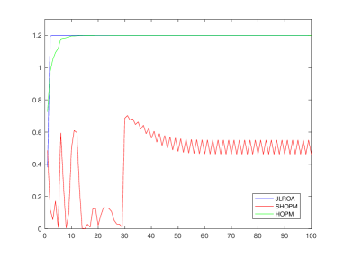
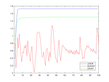
Refer to caption
(a) p=1𝑝1p=1
Refer to caption
(b) p=2𝑝2p=2
Refer to caption
(c) p=3𝑝3p=3

​​​ ​​​

Figure 2: Results of Example 6.2.
Example 6.3.

We randomly generate 1000 tensors in symm(10×10×10)symmsuperscript101010\text{symm}(\mathbb{R}^{10\times 10\times 10}), and run JLROA and Trust region algorithms for them. Denote by JVal and TVal the final value of (2.2) obtained by JLROA and Trust region, respectively. Set the following notations.
(i) NumG::NumGabsent\textsc{NumG}: the number of cases that JVal is greater than TVal;
(ii) NumS::NumSabsent\textsc{NumS}: the number of cases that JVal is smaller than TVal;
(iii) NumE::NumEabsent\textsc{NumE}: the number of cases that JVal is equal777the difference is smaller than 0.0001. to TVal;
(iv) RatioG::RatioGabsent\textsc{RatioG}: the average of JVal/TValJValTVal\textsc{JVal}/\textsc{TVal} when JVal is greater than TVal;
(v) RatioS::RatioSabsent\textsc{RatioS}: the average of JVal/TValJValTVal\textsc{JVal}/\textsc{TVal} when JVal is smaller than TVal.
The results are shown in Table 2 and Figure 3. It can be seen that RatioG is very large when p=1,2𝑝12p=1,2, which means that Turst region is not so stable as JLROA in these two cases. Correspondingly, Trust region algorithm has generally better performance when p>2𝑝2p>2.

Table 2:
NumG NumS NumE RatioG RatioS
p=1𝑝1p=1 125 0 875 211.7822
p=2𝑝2p=2 395 360 245 5.0299 0.9986
p=5𝑝5p=5 431 555 14 1.0016 0.9987
p=8𝑝8p=8 393 604 3 1.0011 0.9992
p=10𝑝10p=10 35 962 3 1.0002 0.9995
Refer to caption
(a) p=1
Refer to caption
(b) p=2
Refer to caption
(c) p=5
Refer to caption
(d) p=8

​​​ ​​​ ​​​

Figure 3: Distributions of points (JVal,TVal)JValTVal(\textsc{JVal},\textsc{TVal}) in Example 6.3. The points are blue when JVal is greater, and red when TVal is greater.
Example 6.4.

Let 𝓐symm(10×10×10)𝓐symmsuperscript101010\boldsymbol{\mathcal{A}}\in\text{symm}(\mathbb{R}^{10\times 10\times 10}) and p=2𝑝2p=2. Suppose that 𝑸subscript𝑸\boldsymbol{Q}_{\ast} is an accumulation point of JLROA-G. To check the frequency of conditions (4.2) and (4.3) being satisfied, we define

ω=min{|𝒲112|,|𝒲122|,|𝒲333|,,|𝒲nnn|},𝜔subscript𝒲112subscript𝒲122subscript𝒲333subscript𝒲𝑛𝑛𝑛\omega=\min\{|\mathcal{W}_{112}|,|\mathcal{W}_{122}|,|\mathcal{W}_{333}|,\cdots,|\mathcal{W}_{nnn}|\},

where 𝓦=𝓐(𝑸)𝓦𝓐subscript𝑸\boldsymbol{\mathcal{W}}=\boldsymbol{\mathcal{A}}(\boldsymbol{Q}_{\ast}). We choose the iteration 𝑸Ksubscript𝑸𝐾\boldsymbol{Q}_{K} as the approximation of an accumulation point when K𝐾K is large enough (K=500𝐾500K=500 in this experiment). We randomly generate 𝓐symm(10×10×10)𝓐symmsuperscript101010\boldsymbol{\mathcal{A}}\in\text{symm}(\mathbb{R}^{10\times 10\times 10}) for 100010001000 times, and run JLROA-G to see the frequency that ω>0𝜔0\omega>0 (greater than 0.0001). The results are shown in Figure 4, where ω>0𝜔0\omega>0 for 991991991 times. It can be seen that the conditions (4.2) and (4.3) are satisfied in most cases.

Refer to caption
Figure 4: Results of Example 6.4. Blue points mean that ω>0𝜔0\omega>0, while red points mean that ω=0𝜔0\omega=0.

References

  • [1] P.-A. Absil, R. Mahony, and R. Sepulchre, Optimization Algorithms on Matrix Manifolds, Princeton University Press, 2008.
  • [2] A. Anandkumar, R. Ge, D. Hsu, S. M. Kakade, and M. Telgarsky, Tensor decompositions for learning latent variable models, Journal of Machine Learning Research, 15 (2014), pp. 2773–2832.
  • [3] J. Bell, The bernstein and nikolsky inequalities for trigonometric polynomials, (2015).
  • [4] N. Boumal, B. Mishra, P.-A. Absil, and R. Sepulchre, Manopt, a matlab toolbox for optimization on manifolds, Journal of Machine Learning Research, 15 (2014), pp. 1455–1459, http://jmlr.org/papers/v15/boumal14a.html.
  • [5] J. Chen and Y. Saad, On the tensor SVD and the optimal low rank orthogonal approximation of tensors, SIAM Journal on Matrix Analysis and Applications, 30 (2009), pp. 1709–1734.
  • [6] A. Cichocki, D. Mandic, L. D. Lathauwer, G. Zhou, Q. Zhao, C. Caiafa, and H. A. PHAN, Tensor decompositions for signal processing applications: From two-way to multiway component analysis, IEEE Signal Processing Magazine, 32 (2015), pp. 145–163.
  • [7] P. Comon, Independent Component Analysis, in Higher Order Statistics, J.-L. Lacoume, ed., Elsevier, Amsterdam, London, 1992, pp. 29–38.
  • [8] P. Comon, Independent component analysis, a new concept?, Signal Processing, 36 (1994), pp. 287–314.
  • [9] P. Comon, Tensor diagonalization, a useful tool in signal processing, IFAC Proceedings Volumes, 27 (1994), pp. 77–82.
  • [10] P. Comon, Tensors: a brief introduction, IEEE Signal Processing Magazine, 31 (2014), pp. 44–53.
  • [11] P. Comon, G. Golub, L.-H. Lim, and B. Mourrain, Symmetric tensors and symmetric tensor rank, SIAM Journal on Matrix Analysis and Applications, 30 (2008), pp. 1254–1279.
  • [12] P. Comon and C. Jutten, eds., Handbook of Blind Source Separation, Academic Press, Oxford, 2010.
  • [13] A. P. da Silva, P. Comon, and A. L. F. de Almeida, A finite algorithm to compute rank-1 tensor approximations, IEEE Sig. Proc. Letters, 23 (2016), pp. 959–963.
  • [14] L. De Lathauwer, Signal processing based on multilinear algebra, Katholieke Universiteit Leuven, 1997.
  • [15] L. De Lathauwer, B. De Moor, and J. Vandewalle, A multilinear singular value decomposition, SIAM Journal on Matrix Analysis and Applications, 21 (2000), pp. 1253–1278.
  • [16] L. De Lathauwer, B. De Moor, and J. Vandewalle, On the best rank-1 and rank-(r1 ,r2 ,. . .,rn) approximation of higher-order tensors, SIAM Journal on Matrix Analysis and Applications, 21 (2000), pp. 1324–1342.
  • [17] V. De Silva and L.-H. Lim, Tensor rank and the ill-posedness of the best low-rank approximation problem, SIAM Journal on Matrix Analysis and Applications, 30 (2008), pp. 1084–1127.
  • [18] M. Ishteva, P.-A. Absil, and P. Van Dooren, Jacobi algorithm for the best low multilinear rank approximation of symmetric tensors, SIAM J. Matrix Anal. Appl., 2 (2013), pp. 651–672.
  • [19] E. Kofidis and P. A. Regalia, On the best rank-1 approximation of higher-order supersymmetric tensors, SIAM Journal on Matrix Analysis and Applications, 23 (2002), pp. 863–884.
  • [20] T. G. Kolda, Orthogonal tensor decompositions, SIAM Journal on Matrix Analysis and Applications, 23 (2001), pp. 243–255.
  • [21] T. G. Kolda and B. W. Bader, Tensor decompositions and applications, SIAM review, 51 (2009), pp. 455–500.
  • [22] T. G. Kolda and J. R. Mayo, Shifted power method for computing tensor eigenpairs, SIAM Journal on Matrix Analysis and Applications, 32 (2011), pp. 1095–1124.
  • [23] J. Li, K. Usevich, and P. Comon, Globally convergent jacobi-type algorithms for simultaneous orthogonal symmetric tensor diagonalization, SIAM Journal on Matrix Analysis and Applications, 39 (2018), pp. 1–22.
  • [24] J. Li, K. Usevich, and P. Comon, On approximate diagonalization of third order symmetric tensors by orthogonal transformations, Linear Algebra and its Applications, 576 (2019), pp. 324–351.
  • [25] H. Lu, K. N. Plataniotis, and A. Venetsanopoulos, Multilinear subspace learning: dimensionality reduction of multidimensional data, Chapman and Hall/CRC, 2013.
  • [26] J. Pan and M. K. Ng, Symmetric orthogonal approximation to symmetric tensors with applications to image reconstruction, Numerical Linear Algebra with Applications, 25 (2018), p. e2180.
  • [27] L. Qi and Z. Luo, Tensor analysis: Spectral theory and special tensors, SIAM, 2017.
  • [28] L. Qi, F. Wang, and Y. Wang, Z-eigenvalue methods for a global polynomial optimization problem, Mathematical Programming, 118 (2009), pp. 301–316.
  • [29] R. Schneider and A. Uschmajew, Convergence results for projected line-search methods on varieties of low-rank matrices via lojasiewicz inequality, SIAM Journal on Optimization, 25 (2015), pp. 622–646.
  • [30] N. D. Sidiropoulos, L. De Lathauwer, X. Fu, K. Huang, E. E. Papalexakis, and C. Faloutsos, Tensor decomposition for signal processing and machine learning, IEEE Transactions on Signal Processing, 65 (2017), pp. 3551–3582.
  • [31] A. Smilde, R. Bro, and P. Geladi, Multi-way analysis with applications in the chemical sciences, Wiley, (2004).
  • [32] K. Usevich, J. Li, and P. Comon, Approximate matrix and tensor diagonalization by unitary transformations: convergence of jacobi-type algorithms, arXiv:1905.12295, (2019).
  • [33] T. Zhang and G. H. Golub, Rank-one approximation to high order tensors, SIAM Journal on Matrix Analysis and Applications, 23 (2001), pp. 534–550.
  • [34] X. Zhang, C. Ling, and L. Qi, The best rank-1 approximation of a symmetric tensor and related spherical optimization problems, SIAM Journal on Matrix Analysis and Applications, 33 (2012), pp. 806–821.
  • [35] X. Zhang, L. Qi, and Y. Ye, The cubic spherical optimization problems, Mathematics of computation, 81 (2012), pp. 1513–1525.