Global Adaptive Generative Adjustment

Abstract

Many traditional signal recovery approaches can behave well basing on the penalized likelihood. However, they have to meet with the difficulty in the selection of hyperparameters or tuning parameters in the penalties. In this article, we propose a global adaptive generative adjustment (GAGA) algorithm for signal recovery, in which multiple hyperpameters are automatically learned and alternatively updated with the signal. We further prove that the output of our algorithm directly guarantees the consistency of model selection and signal estimate. Moreover, we also propose a variant GAGA algorithm for improving the computational efficiency in the high-dimensional data analysis. Finally, in the simulated experiment, we consider the consistency of the outputs of our algorithms, and compare our algorithms to other penalized likelihood methods: the Adaptive LASSO, the SCAD and the MCP. The simulation results support the efficiency of our algorithms for signal recovery, and demonstrate that our algorithms outperform the other algorithms.

1 Introduction

In the past two decades, signal recovery methods developed rapidly in the machine learning and statistics community. Much of the recent work push the boundaries of our theoretical knowledge on the high-dimensional data analysis, and offers a wide range of applications in the computer, biology and medicine fields. Specially, several important approaches (Tibshirani, 1996; Chen et al., 1998; Fan & Li, 2001; Candès & Tao, 2005; Zhao & Yu, 2006) have been developed for the rapid development in signal recovery; see Hastie et al., 2009 for an overview.

Though demonstrated effective in theoretical analysis, the performance of the signal recovery relies on an appropriate choice of the tuning parameters in the penalized likelihood. The single tuning parameter selection has been studied in a series of works using the BIC-type scoring criterions (Wang et al. (2007, 2009); Fan & Tang (2013); Hui et al. (2015)). To conquer the oracle limitation of the LASSO (Tibshirani (1996)), Zou (2006) proposed an adaptive version by introducing multiple hyperparamters for customizing a personalized shrinkage for each component in signal. In the practical computation, the adaptive LASSO considers the selection for a pair of hyperparameters by the cross-validation (CV). Other penalized likelihood methods: the SCAD (Fan & Li (2001)) and the MCP (Zhang (2010)) also need to choose two hyperparameters over the two-dimensional grids using some scoring criteria.

To our best knowledge, there is no existing work accommodating the selection directly for the multiple tuning parameters. The traditional scoring search is not efficient any more since it incurs huge time-cost for the passive traveral in multi-dimensional threshold space. Moreover, most theorectical properties on those penalized methods are based on the optimal solution of the objective function rather than the output of their algorithms. The gap between the optimal solution and the output could make the performance of their algorithms deviating from those expected theoretical properties.

Our present work contributes three novel points in the signal recovery: Firstly, our proposed algorithm can alternatively update the signal and multiple hyperparameters in an active way. It provides an automatic learning of hyperparameters for signal recovery. Secondly, we prove that the ouput of the algorithm enjoys both the consistency for model selection and signal estimate. Thirdly, our proposed algorithm works in a concise form and performs well on both the error and the accuracy of the signal estimate in the computational aspect.

In our work, multiple tuning parameters are introduced for personalising the penalty on each component in the signal. Tuning parameters and the signal are alternatively updated by a data-driven method, which we call as global adaptive generative adjustment (GAGA). The GAGA updates multiple hyperparameters in a purposeful way. So it avoids the time-consuming scoring searching in the traditional hyperparameter selection. By studying in detailed the iteration process of algorithm, we prove that the output of the GAGA algorithm directly possesses the consistency of both the model selection and the signal estimate. Thus the output of the algorithm usually has a performance with a low error and a high accuracy when the sample size is large enough. Furthermore, we propose another QR-decomposition version of the GAGA algorithm. This QR-version can improve the computational efficiency of the orignal one for the high-dimensional data analysis. We illustrate the performance of our algorithms by several simulated experiments. Our algorithms outperform other penalized likelihood methods on the error and the accuracy of the signal estimate. The time costs are also much lower of our algorithms than the others with the 10-fold Cross-Validation selection.

The rest of our paper is organized as follows. In Section 2, we describe two versions of the Global Adaptive Generative Adjustment algorithm. and present the theoretical guarantee of our algorithm. In Section 3, we show the simulation results of our algorithms and other popular penalized likelihood algorithms. Finally, we give the conclusion on our algorithms in Section 4. All the proof details are put into the Supplementary Material.

2 Global Adaptive Generative Adjustment

In this section, we describe the Global Adaptive Generative Adjustment (GAGA) algorithm, and present the theoretical guarantees of the algorithm on a linear model with an orthogonal design matrix. Furthermore, we propose a QR-decomposition version of the GAGA algorithm for improving its computational efficiency in the high-dimensional data analysis.

2.1 A Start From A Simple Linear Model

We start from a linear model $\mathbf{y}=\mathbf{X}\bm{\beta}^{*}+\bm{\varepsilon}$, where the true signal $\bm{\beta}^{*}=(\beta_{1}^{*},\cdots,\beta_{p}^{*})^{T}$, the noise $\bm{\varepsilon}\sim N(\mathbf{0},\sigma^{2}\mathbf{I})$ and $\mathbf{I}$ is an identity matrix. The recovery of the true signal $\bm{\beta}^{*}$ can be considered under a shrinkage framework with multiple tuning parameters. For getting a concise update form, we first assume that the variance $\sigma^{2}=1$. So $\bm{\varepsilon}\sim N(\mathbf{0},\mathbf{I})$. Specifically, we take into account the ridge regression form

$$\frac{1}{2}\|\mathbf{y}-\mathbf{X}\bm{\beta}\|^{2}+\frac{1}{2}\sum_{j=1}^{p}\lambda_{j}{\beta_{j}}^{2}$$

with tuning parameters $\lambda_{j}$, $j=1,\cdots,p$. The tuning parameter $\lambda_{j}$ customizes the amount of the penalty on the coefficient $\beta_{j}$. It can provide a personalized shrinkage on the coefficient. We introduce a global adaptive generative adjustment (GAGA) algorithm 1 to recover a true signal $\bm{\beta}^{*}$. In case that the variance is unknown, it can be estimated by using the residual of the estimated signal. We will give the whole algorithm version with the estimated noise in the last part of this subsection.

In the algorithm, tuning parameters and the signal are alternatively updated by a data-driven method. So it avoids the time-consuming scoring searching in the traditional hyperparameter selection. The inputs of this algorithm are the response vector $\mathbf{y}$, the design matrix $\mathbf{X}$, the iteration number $K$ and a constant $\alpha$. The constant $\alpha$ can control the sparsity of the signal estimate. We set $\alpha=2$ in the whole simulation experiment part. The output of this algorithm is the signal estimate $\hat{\bm{\beta}}=\text{GAGA}(\mathbf{y},\mathbf{X},K,\alpha)$.

As shown in Algorithm 1, the estimate on the signal $\bm{\beta}^{*}$ is updated by a ridge regression form in Line 3. This regression relies on a diagonal matirx $\bm{\Lambda}$. Its diagonal elements are those personalized tuning parameters, which are updated in Line 4. The tuning parameter vector $\bm{\lambda}$ obtains a global adaptive update form in Line 4 depending on the data $\mathbf{X}$ and $\mathbf{y}$. Furthermore, the vector $\bm{\lambda}$ can provide a generative adjustment for the signal estimate in the next iteration shown in Line 3. After $K$ iterations, we judge a hard truncation condition in Line 9. The condition determines that the estimated coefficient $\hat{\beta}_{j}^{(K)}$ is shrinked to zero or not.

Algorithm 1 Global Adaptive Generative Adjustment (GAGA)

Input: Response vector $\mathbf{y}$, design matrix $\bm{X}$, iteration number $K$, growth factor $\alpha$.
Output: The signal estimate $\hat{\bm{\beta}}^{*}=(\hat{\beta}_{1}^{*},\cdots,\hat{\beta}_{p}^{*})$.
Main Procedure:

1:  Hyperparameter vector $\bm{\lambda}^{(1)}=(\lambda_{1}^{(1)},\cdots,\lambda_{p}^{(1)})^{T}=\mathbf{0}$.

2:  for $k=1,2,\ldots K-1$ do

3:     $\hat{\bm{\beta}}^{(k)}=(\mathbf{X}^{T}\mathbf{X}+\bm{\Lambda}^{(k)})^{-1}\mathbf{X}^{T}\mathbf{y}$ where $\bm{\Lambda}^{(k)}=diag(\bm{\lambda}^{(k)})$.

4:     $\lambda_{j}^{(k+1)}=\frac{\alpha}{(\hat{\beta}_{j}^{(k)})^{2}+((\mathbf{X}^{T}\mathbf{X}+\bm{\Lambda}^{(k)})^{-1})_{jj}}$, $j=1,\cdots,p$.

5:  end for

6:  $\bm{\lambda}^{(K)}=\bm{\lambda}^{(K)}/\alpha$.

7:  $\hat{\bm{\beta}}^{(K)}=(\mathbf{X}^{T}\mathbf{X}+\bm{\Lambda}^{(K)})^{-1}\mathbf{X}^{T}\mathbf{y}$ where $\bm{\Lambda}^{(K)}=diag(\bm{\lambda}^{(K)})$.

8:  for $j=1,2,\ldots p$ do

9:     if $(\hat{\beta}_{j}^{(K)})^{2}\leq((\mathbf{X}^{T}\mathbf{X})^{-1})_{jj}-((\mathbf{X}^{T}\mathbf{X}+\bm{\Lambda}^{(K)})^{-1})_{jj}$ then

10:        $\hat{\beta}_{j}^{*}\leftarrow 0$.

11:     else

12:        $\hat{\beta}_{j}^{*}\leftarrow\hat{\beta}_{j}^{(K)}$.

13:     end if

14:  end for

In the following part of this subsection, we show the theorectical guarantees on the output of the GAGA algorithm when the design matrix is column orthogonal. Those guarantees illustrate that the GAGA algorithm can provide an efficient estimate on the signal under some conditions. The empirical performance of the GAGA will be shown in Section 3.

We denote $\mathcal{Q}$ as the subscript set $\{j|\beta_{j}^{*}\neq 0\}$ for non-zero components of signal. Assume that the design matrix $\mathbf{X}=(\textbf{x}_{1},\cdots,\textbf{x}_{p})$ is column orthogonal. That is $\mathbf{X}^{T}\mathbf{X}=diag((a_{1},\cdots,a_{p}))$. And further assume that the condition number $\kappa=\frac{\max_{j}a_{j}}{\min_{j}a_{j}}$ is bounded. Since the column orthogonality of $\mathbf{X}$, the diagonal element $((\mathbf{X}^{T}\mathbf{X}+\bm{\Lambda}^{(k)})^{-1})_{jj}=(a_{j}+\lambda_{j}^{(k)})^{-1}$. So the update of $\lambda_{j}^{(k+1)}$ in Line 4 of the GAGA algorithm can be computed by $\frac{\alpha(\lambda_{j}^{(k)}+a_{j})^{2}}{\lambda_{j}^{(k)}+a_{j}+z_{j}}$ where $z_{j}=(\textbf{x}_{j}^{T}\textbf{y})^{2}$. Moreover, the hard thresholding condition in Line 9 becomes $(\hat{\beta}_{j}^{(K)})^{2}\leq a_{j}^{-1}-(a_{j}+\lambda_{j}^{(K)})^{-1}$. Unlike the conventional discussion on the optimum of the penalized likelihood, we prove that the output of our GAGA algorithm directly satisfies the consistency of model selection and signal estimate.

For any convergent subsequence $\{\bm{\lambda}^{(k_{l})}\}_{l}$ of the updated hyperparameter sequence $\{\bm{\lambda}^{(k)}\}_{k}$, denote $\bm{\lambda}^{\infty}$ as the limit $\lim\limits_{l\rightarrow\infty}\bm{\lambda}^{(k_{l})}$ (Components of the limit are allowed to be the infinity). Let $\bm{\lambda}^{*}=\bm{\lambda}^{\infty}/\alpha$, $\bm{\Lambda}^{*}=diag(\bm{\lambda}^{*})$, and $\hat{\bm{\beta}}=(\mathbf{X}^{T}\mathbf{X}+\bm{\Lambda}^{*})^{-1}\mathbf{X}^{T}\mathbf{y}$. Furthermore, let $\hat{\bm{\beta}}^{*}$ be the personalized thresholding of $\hat{\bm{\beta}}$ in the GAGA algorithm. Theorem 2.1 illustrates the effectiveness of the hard truncation in Line 10 of the GAGA algorithm. If the true coefficient is zero, the hard truncation happens with a high probability when the sample size is large enough. It means that the zero-coefficient position can be correctly detected with a high probability.

Theorem 2.1.

Assume that the design matrix is column orthogonal. We have that the probability for personalized thresholding in $\mathcal{Q}^{c}$

$$\mathbb{P}(\bigcap\limits_{j\in\mathcal{Q}^{c}}\{(\hat{\beta}_{j})^{2}\leq a_{j}^{-1}-(a_{j}+\lambda_{j}^{*})^{-1}\})$$

$$\geq 1-\exp(-\frac{1}{2}(\sqrt{\alpha}+\sqrt{\alpha-1})^{2}+\log(p-q))$$

Moreover, for any $0<\eta<1$, the probability for no personalized thresholding in $\mathcal{Q}$

$$\mathbb{P}(\bigcap\limits_{j\in\mathcal{Q}}\{(\hat{\beta}_{j})^{2}>a_{j}^{-1}-(a_{j}+\lambda_{j}^{*})^{-1}\})$$

$$\geq 1-2\exp(-\frac{1}{2}(\min\limits_{j\in\mathcal{Q}}a_{j}^{1/2}|\beta_{j}|-(\sqrt{\alpha}+\sqrt{\alpha-1}))^{2}+$$

$$\log(q))-\exp(-\frac{1}{2}((1-\eta)\min\limits_{j\in\mathcal{Q}}a_{j}^{1/2}|\beta_{j}^{*}|-$$

$$(\sqrt{\alpha}+\sqrt{\alpha-1}))^{2}+\log(q))$$

when the inequalities $\eta^{2}\min\limits_{j\in\mathcal{Q}}a_{j}{\beta_{j}^{*}}^{2}\geq\frac{1}{\sqrt{\alpha}+\sqrt{\alpha-1}-1}$ and $(1-\eta)\min\limits_{j\in\mathcal{Q}}a_{j}^{1/2}|\beta_{j}^{*}|-(\sqrt{\alpha}+\sqrt{\alpha-1})\geq 0$ hold.

The following Theorem 2.2 provides an error expectation bound for the output $\hat{\bm{\beta}}^{*}$ of the GAGA algorithm. Let the event $E=\{z_{j}<(\sqrt{\alpha}+\sqrt{\alpha-1})^{2}a_{j},j\in\mathcal{Q}^{c}\}$, the event $F=\{\max\limits_{j\in\mathcal{Q}}\lambda_{j}^{*}{\beta_{j}^{*}}^{2}\leq\frac{1}{\eta^{2}}\}$ where $0<\eta<1$, and the condition number $\kappa=\frac{\max_{j}a_{j}}{\min_{j}a_{j}}$.

Theorem 2.2.

Assume that the design matrix is column orthogonal, and the condition number $\kappa$ is bounded. We have that

$$\mathbf{E}\|\hat{\bm{\beta}}^{*}-\bm{\beta}^{*}\|$$

$$\leq \sqrt{\frac{q}{\min\limits_{j\in\mathcal{Q}}a_{j}}}(1+\sqrt{\kappa}+\frac{1}{\eta^{2}\min\limits_{j\in\mathcal{Q}}a_{j}^{1/2}|\beta_{j}^{*}|})+$$

$$(E\|\hat{\bm{\beta}}\|^{2})^{1/2}(2(\mathbb{P}(E^{c}))^{1/2}+(\mathbb{P}(F^{c}))^{1/2})+$$

$$\|\bm{\beta}^{*}\|(\mathbb{P}(E^{c})+\mathbb{P}(F^{c})).$$

Moreover, we have that

$$\mathbb{E}\|\hat{\bm{\beta}}^{*}-\bm{\beta}^{*}\|\xrightarrow{\alpha\rightarrow\infty,\min\limits_{j\in\mathcal{Q}}a_{j}\rightarrow\infty}0$$

if further $q=o(\min\limits_{j\in\mathcal{Q}}a_{j})$, $\log(p)+\log(\frac{p}{\min\limits_{j}a_{j}}+\|\bm{\beta}^{*}\|^{2})=o(\alpha)$ and $\alpha=o(\min\limits_{j\in\mathcal{Q}}a_{j}{\beta_{j}^{*}}^{2})$.

All the techinial details can be found in the Supplementary Material. In the following subsection, we will propose a QR-decomposition version of the GAGA algorihm for the high-dimensional data analysis. Moreover, we will find that this new version is compatible with our developed theory under the orthogonal design assumption.

In case that the variance is unknown, we actually can estimate the variance in each iteration by the residual of the estimated signal:

$$(\sigma^{2})^{(k+1)}=(\mathbf{X}\hat{\bm{\beta}}^{(k)}-\mathbf{y})^{T}(\mathbf{X}\hat{\bm{\beta}}^{(k)}-\mathbf{y})/N$$ (1)

or

$$(\sigma^{2})^{(k+1)}= \frac{1}{N}\bigg{(}\mathbf{y}^{T}\mathbf{y}-2\hat{\bm{\beta}}^{(k)T}\mathbf{X}^{T}\mathbf{y}+$$ (2)

$$\text{tr}\big{(}(\hat{\bm{\beta}}^{(k)T}\hat{\bm{\beta}}^{(k)}+\mathbf{D}^{(k)})\mathbf{X}^{T}\mathbf{X}\big{)}\bigg{)}$$

where $\mathbf{D}^{(k)}=(\sigma^{2})^{(k)}(\mathbf{X}^{T}\mathbf{X}+(\sigma^{2})^{(k)}\bm{\Lambda}^{(k)})^{-1}$. Correspondingly, the hard truncation condition turns into the inequality:

$$(\hat{\beta}_{j}^{(K)})^{2}< (\sigma^{2})^{(K)}((\mathbf{X}^{T}\mathbf{X})^{-1})_{jj}-$$ (3)

$$(\sigma^{2})^{(K)}((\mathbf{X}^{T}\mathbf{X}+(\sigma^{2})^{(K)}\bm{\Lambda}^{(K)})^{-1})_{jj}$$

Algorithm 2 Global Adaptive Generative Adjustment (GAGA) with Estimated Variance

Input: the response vector $\mathbf{y}$, the design matrix $\bm{X}$, the iteration number $K$, the constant $\alpha$.
Output: the signal estimate $\hat{\bm{\beta}}^{*}$.
Main Procedure:

1:  $\bm{\lambda}^{(1)}=(\lambda_{1}^{(1)},\cdots,\lambda_{p}^{(1)})^{T}=\mathbf{0}$, $(\sigma^{2})^{(1)}=1$.

2:  for $k=1,\ldots,K-1$ do

3:     $\hat{\bm{\beta}}^{(k)}=(\mathbf{X}^{T}\mathbf{X}+(\sigma^{2})^{(k)}\bm{\Lambda}^{(k)})^{-1}\mathbf{X}^{T}\mathbf{y}$ where $\bm{\Lambda}^{(k)}=diag(\bm{\lambda}^{(k)})$.

4:     $\lambda_{j}^{(k+1)}=\frac{\alpha}{(\hat{\beta}_{j}^{(k)})^{2}+(\sigma^{2})^{(k)}((\mathbf{X}^{T}\mathbf{X}+(\sigma^{2})^{(k)}\bm{\Lambda}^{(k)})^{-1})_{jj}}$ where $j=1,\cdots,p$.

5:     Update $(\sigma^{2})^{(k+1)}$ by the equation (2).

6:  end for

7:  $\bm{\lambda}^{(K)}=\bm{\lambda}^{(K)}/\alpha$

8:  $\hat{\bm{\beta}}^{(K)}=(\mathbf{X}^{T}\mathbf{X}+(\sigma^{2})^{(K)}\bm{\Lambda}^{(K)})^{-1}\mathbf{X}^{T}\mathbf{y}$ where $\bm{\Lambda}^{(K)}=diag(\bm{\lambda}^{(K)})$.

9:  for $j=1,2,\ldots p$ do

10:     if the inequality (3) holds, then

11:        $\hat{\beta}_{j}^{*}\leftarrow 0$.

12:     else

13:        $\hat{\beta}_{j}^{*}\leftarrow\hat{\beta}_{j}^{(K)}$.

14:     end if

15:  end for

2.2 Another Version of the GAGA Algorithm

Since the GAGA computes the matrix inversion in each iteration, the efficency of the algorithm may be limited for the high-dimensional data. So we further propose a variant version GAGA_QR for dealing with this problem. This version first roughly estimates the signal vector by the least-square solution $\bm{\gamma}=(\mathbf{X}^{T}\mathbf{X})^{-1}\mathbf{X}^{T}\mathbf{y}$. And then sort the coefficients of $\bm{\gamma}$ in a decreasing absolute value ordering. When the sample size is large enough, the sorted estimate $\bm{\gamma}$ could be an apropriate approximation of the true signal $\bm{\beta}^{*}$, whose zero coefficients are arranged in the tail part. Permutate the columns of the design matrix $\mathbf{X}$ by $\mathbf{X}_{\text{new}}=\mathbf{X}\mathbf{P}$, where $\mathbf{P}$ is a permutation matrix according to the rearrangement of those coefficients in $\bm{\gamma}$. Do the QR-decomposition on the permuted design matrix $\mathbf{X}_{\text{new}}=\mathbf{Q}\mathbf{R}$, where $\mathbf{Q}$ is a column orthogonal matrix and $\mathbf{R}$ is an upper triangular matrix. Under the QR-decomposition, the original linear model can be viewed as $\mathbf{y}=\mathbf{Q}\bm{\mathbf{\theta}}+\bm{\epsilon}$, where $\bm{\theta}=\mathbf{R}\bm{\beta}^{*}$. Furthermore, we use the GAGA algorihtm for the response vector $\mathbf{y}$ and the new design matrix $\mathbf{Q}$. The final signal estimate is obtained by $\mathbf{P}*\mathbf{R}^{-1}*\text{GAGA}(\mathbf{y},\mathbf{Q},K,\alpha)$, where $K$ is the iteration number and $\alpha$ is a constant.

Algorithm 3 Global Adaptive Generative Adjustment Using QR-Decomposition (GAGA_QR)

Input: the response vector $\mathbf{y}$, the design matrix $\bm{X}$, the iteration number $K$, the constant $\alpha$
Output: the signal estimate $\hat{\bm{\beta}}^{*}$
Main Procedure:

1:  Compute the least-square estimate$\bm{\gamma}=(\mathbf{X}^{T}\mathbf{X})^{-1}\mathbf{X}^{T}\mathbf{y}$.

2:  Sort elements of $\bm{\gamma}$ in a decreasing absolute value order.

3:  Rearrange the columns of $\mathbf{X}$ by $\mathbf{X}_{\text{new}}=\mathbf{X}\mathbf{P}$, where $\mathbf{P}$ is a permutation matrix according to the decreasing absolute value order of $\bm{\gamma}$.

4:  Use the QR-decomposition for $\mathbf{X}_{\text{new}}$. Let $\mathbf{X}_{\text{new}}=\mathbf{Q}\mathbf{R}$ where $\mathbf{Q}$ is a column orthogonal matrix and $\mathbf{R}$ is an upper triangular matrix.

5:  Compute $\bm{\theta}$=GAGA(y,Q,$K$,$\alpha$) by using the GAGA algorithm

6:  The estimate signal $\hat{\bm{\beta}}^{*}=\mathbf{P}\mathbf{R}^{-1}\bm{\theta}$.

Since the matrix $\mathbf{R}$ is an upper triangular matrix, so does the matrix $\mathbf{R}^{-1}$. If the estimate $\bm{\gamma}$ captures the correct rearrangement matrix $\mathbf{P}$ such that the true signal $\bm{\beta}^{*}$ with zero coefficients in its tail, the linear transform $\bm{\theta}=\mathbf{R}\bm{\beta}^{*}$ maintains the sparse tail part as $\bm{\beta}^{*}$ since $\mathbf{R}$ is an upper triangular matrix. Moreover, the inverse linear tranform $\mathbf{R}^{-1}\bm{\theta}$ also keeps the sparse structure in the tail part as $\bm{\theta}$. So the GAGA_QR is efficient once the GAGA successfully finds those zero coefficients in the signal.

Note that in the GAGA_QR algorithm, the inversion of matrix $\mathbf{X}^{T}\mathbf{X}$ is only computed once in Line 1. Since the column orthogonality of $\mathbf{Q}$, the inversion computation is easy in the GAGA algorithm with the inputs $\mathbf{y}$, $\mathbf{Q}$, $K$ and $\alpha$. Though another matrix inversion is asked in Line 6 of the GAGA_QR, the computation is also easy since the matrix $R$ is an upper traingular matrix. The computation on $(\mathbf{X}^{T}\mathbf{X})^{-1}$ is only doned once in the GAGA_QR algorithm, while the GAGA algorithm has to compute the inversion matrix $(\mathbf{X}^{T}\mathbf{X}+\bm{\Lambda}^{k})^{-1}$ in each iteration. So the GAGA_QR algorithm takes less time costs than the GAGA algorithm, especially when we cope with a high-dimensional design matrix $\mathbf{X}$ with a large number of columns. The experiment on the comparison between the GAGA and the GAGA_QR will be shown in the next section.

3 Simulation

In this section, we do experiments to show the performances of our algorithms on the simulated data. We first compare our algorithms to the SCAD ((Fan & Li, 2001)), the adaptive LASSO ((Zou, 2006)) and the MCP ((Zhang, 2010)) on two models, whose sparse structures are from (Tibshirani, 1996). We further design another model for testing them on high-dimensional data. And then, we demonstrate their performances on the asymptotic property of those estimates as the sample size increases. Finally, we show the time costs of our algorithms on the high-dimensional data analysis.

Their performances are evaluated by the error (ERR) and the accuracy (ACC). The ERR is computed with $\|\hat{\bm{\beta}}-\bm{\beta}^{*}\|$ on the value difference between the estimated and true one. The ACC is defined by the ratio $\frac{\text{True positives}+\text{True negatives}}{Positives+Negatives}$ of correctly finding the positions of zeros and non-zeros in the true signal $\bm{\beta}^{*}$.

The adaptive LASSO, the SCAD and the MCP are executed in the R with the ncvreg library (Breheny & Huang, 2011). All the experiments in R adopt the OpenBlas for performing basic vector and matrix operations. For these penalized likelihood algorithms, extra tuning parameters are needed to estimate the parameter and regularize the model selection. We consider to set $100$ values for the tuning parameter in the adaptive LASSO, the MCP and the SCAD respectively, and use the $10$-fold Cross-Validation to select the appropriate tuning parameters for them. We further demonstrate their performance by averaging the ERR and the ACC on each value point of the tuning parameter. In the simulation, the iteration number $K$ is set to $50$ and the constant $\alpha=2$ for the GAGA and the GAGA_QR.

(a) Performances on ERR

(b) Performances on ACC

Figure 1: Consider the ERR and the ACC seperately on Model $1$.

Figure 2: Consider the ERR and the ACC comprehensively on Model $1$.

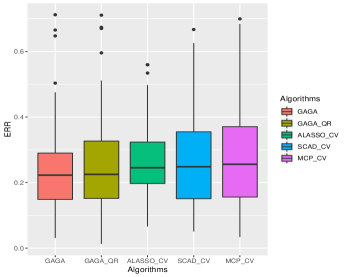
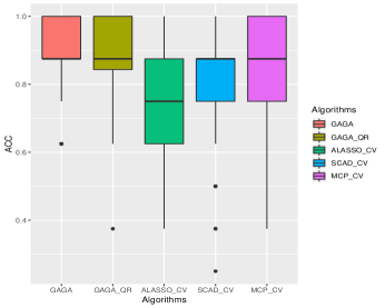
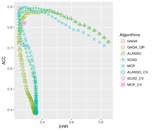
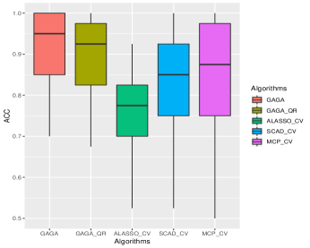
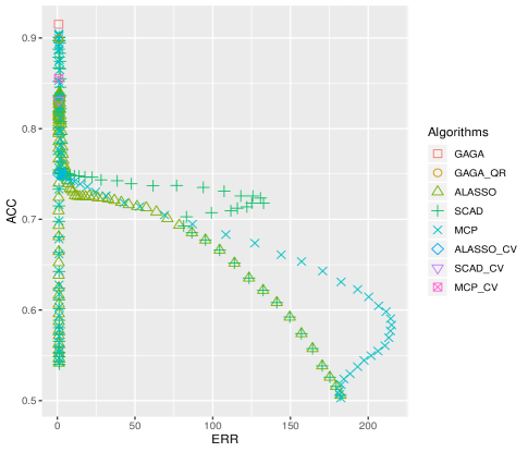
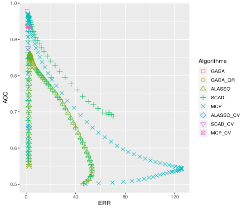
For the Model $1$, $100$ data sets are simulated and each consists of $100$ observations from the linear model $y=\mathbf{x}^{T}\bm{\beta}^{*}+\varepsilon$. The noise $\varepsilon$ is a standard normal random variable. The correlation between $x_{i}$ and $x_{j}$ is $\rho^{|i-j|}$ with $\rho=0.5$. The true signal is set to $\bm{\beta}^{*}=(\beta_{1}^{*},\beta_{2}^{*},0,0,\beta_{3}^{*},0,0,0)^{T}$. The non-zero coefficients $\beta_{1}^{*},\beta_{2}^{*},\beta_{3}^{*}$ are randomly generated from $U(0,1)$. The comparisons between ours and those algorithms are shown in Figure 1. For both the ERR and the ACC, the GAGA algorithm outperforms the adaptive LASSO, the SCAD and the MCP with the $10$-fold CV selection. Furthermore, we plot Figure 2 to comprehensively demonstrate the performance of algorithms on the ERR and the ACC. Each point in Figure 2 represents an average ACC and ERR of $100$ data sets. The performances of the GAGA, the GAGA_QR, the ALASSO_CV, the SCAD_CV and the MCP_CV are characterized by five points. For the adaptive LASSO, the SCAD and the MCP, each algorithm have $100$ points representing the average performance on $100$ values of the tuning parameter. The two points for our algorithms are in the top left corners of Figure 2. They perform better than other algorithms when comprehensively considering the ERR and the ACC. Though the SCAD_CV and the MCP_CV behave well, they do not reach the best ones, which can be obtained by going over the values of the tuning paramter when knowing the ERR and the ACC. Since the true signal is unknown, it is not practical to select the tuning parameter by computing the ERR and the ACC, while our algorithms automatically learn all the tuning parameters and achieve a signal estimate with a low error and a high accuracy.

(a) Performances on ERR

(b) Performances on ACC

Figure 3: Consider the ERR and the ACC seperately on Model $2$.

Figure 4: Consider the ERR and the ACC comprehensively on Model $2$.

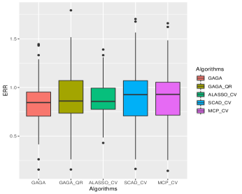
For the Model $2$, $100$ data sets are simulated, and each had $100$ observations from the linear model $y=\mathbf{x}^{T}\bm{\beta}^{*}+\varepsilon$. The noise $\varepsilon$ is a standard normal random variable. For any $i\neq j$, $x_{i}$ and $x_{j}$ have a pairwise correlation of $0.5$. The true coefficient vector

$$\bm{\beta}^{*}=(0,\cdots,0,\beta_{1}^{*},\cdots,\beta_{1}^{*},0,\cdots,0,\beta_{2}^{*},\cdots,\beta_{2}^{*})^{T},$$

there being $10$ repeats in each block. The non-zero components $\beta_{1},\beta_{2}$ are randomly generated from $\beta_{1}\sim U(0,1)$ and $\beta_{2}\sim U(10,100)$ respectively. As shown in Figure 3, for the ACC, the GAGA and the GAGA_QR outperform the adaptive LASSO, the SCAD and the MCP with the $10$-fold CV selection. For the ERR, the GAGA performs better than the adaptive LASSO, the SCAD and the MCP. As shown in Figure 4, our algorithms also perform better than other penalized likelihood algorithms with the CV when comprehensively considering the ERR and the ACC. We also set $100$ values of the tuning parameter in the adaptive LASSO, the MCP and the SCAD respectively. So there are $100$ points in Figure 4 for each penalized likelihood algorithm, and each point represents an average ACC and ERR of algorithms on $100$ data sets. The performance of the GAGA is still beyond those penalized likelihood algorithms with the hyperparameter selection in $100$ values even if knowing the true ERR and ACC.

(a) Performances on ERR

(b) Performances on ACC

Figure 5: Consider the ERR and the ACC seperately on the high-dimensional data.

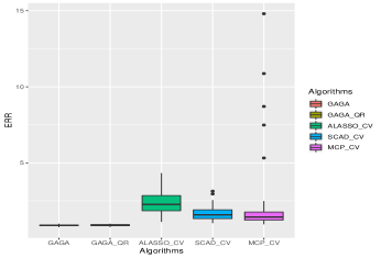
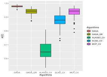
For testing algorithms’ performances on high-dimensional data, we simulate $100$ data sets from the linear model $y=\mathbf{x}^{T}\bm{\beta}^{*}+\varepsilon$. The true signal $\bm{\beta}^{*}$ has $500$ coefficients with $250$ zeros, whose positions are randomly generated in each data set. The non-zero coefficient is randomly generated from $U(0,5)$. Each data set consists of $1000$ observations. For any $i\neq j$, $x_{i}$ and $x_{j}$ have a pairwise correlation of $0.5$. The noise $\varepsilon$ is a standard normal random variable. Figures 5 and 6 illustrate that the GAGA also outperforms other penalized likelihood methods on the ERR and the ACC for the high-dimensional data.

Figure 6: Consider the ERR and the ACC comprehensively on the high-dimensional data.

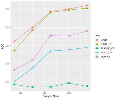
In the next experiment, we further consider the consistentcy of the output of algorithms as the sample size increases. The data is also generated from a linear model $y=\mathbf{x}^{T}\bm{\beta}^{*}+\varepsilon$, where the noise $\varepsilon$ is a standard normal random variable. The signal $\bm{\beta}^{*}$ has eight components. The number of non-zero coefficients in $\bm{\beta}$ is fixed to three, but the non-zero positions are random sampled. $100$ data sets are simulated on each sample size varying in $\{30,60,90,120,150\}$. We compute the average ERR and the average ACC for all the algorithms. For the adaptive LASSO, the SCAD and the MCP, we adopt the $10$-fold CV to select an appropriate tuning parameter for further signal estimates. The simulation result is shown in Figure 7. As the sample size increases, the ERR of our algorithms goes down, and the ACC goes up. Moreover, the GAGA and the GAGA_QR outperform other algorithms on the average ERR and the average ACC of $100$ data sets.

(a) Performances on ERR

(b) Performances on ACC

Figure 7: The performance on the consistency of all the algorithms.

Finally, we compare the time costs between our algorithms and the adaptive LASSO, the SCAD, the MCP with $10$-fold Cross-Validation for the high-dimensional linear model. The dimension of the signal varies in $\{500,1000,2000\}$, the sample size is fixed to $4000$, and the experiment is repeated $10$ times for each dimension. Since the GAGA involves loops of the matrix’s inversion, its time cost depends on the software’s computational efficiency for numerical linear algebra. So we consider to execute the GAGA in both the Matlab and the R. The adaptive LASSO, the SCAD and the MCP are executed in the R with the ncvreg library (Breheny & Huang, 2011). All the experiments in R adopt the OpenBlas for performing basic vector and matrix operations. As demenstrated in Table 1, the GAGA_QR in Matlab has the lowest average time costs on all the dimensions, and the SCAD has the highest ones. Even if considering the time costs only in R, the GAGA and the GAGA_QR also outperform the other algorithms since those penalized likelihood methods have to go over all possible values of hyperparameter to pick up an appropriate one with the 10-fold CV. This experiment runs on a desktop with Intel i7 4.0 GHZ and 32 GB memory.

Table 1: The average time cost of the GAGA, the GAGA_QR, the adaptive LASSO, the SCAD and the MCP.

Dimension	$500$	$1000$	$2000$
GAGA(in Matlab)	0.36s	1.68s	9.34s
GAGA_QR(in Matlab)	0.15s	0.48s	1.74s
GAGA(in R)	3.04s	11.5s	66.67s
GAGA_QR(in R)	1.45s	5.09s	19.39s
ALASSO_CV(in R)	27.36s	54.12s	108.89s
SCAD_CV(in R)	43.37s	103.13s	221.37s
MCP_CV(in R)	25.38s	65.11s	152.51s

4 Conclusion

In this paper, we propose an algorithm named GAGA for the signal recovery. This GAGA algorithm can automatically learn the hyperparamters, and update those hyperparameters and the signal in an alternative way. A variant algorithm called as GAGA_QR is also suggested by using the QR-decompostion for improving the computational efficiency in the high dimensional analysis. In the theoretical part, we prove that the output of the GAGA algorithm can correctly find the positions of zero-coefficient with a high probability, and also provide a consistent estimate on the nonzero coefficients. In the simulation part, the experiment results illustrate that our algorithms outperform the adaptive Lasso, the SCAD and the MCP. Though the GAGA algorithm in this work is dedicated to the linear model, the mechanism behind the global adaptive generative adjustment strategy can be generalized to other statistical models. Exploration of this research direction is underway.

References

- Breheny & Huang (2011) Breheny, P. and Huang, J. Coordinate descent algorithms for nonconvex penalized regression with applications to biological feature selection. Annals of Applied Statistics, 5:232–253, 2011.
- Candès & Tao (2005) Candès, E. J. and Tao, T. The dantzig selector: statistical estimation when p is much larger than n. Annals of Statistics, 35:2313—2351, 2005.
- Chen et al. (1998) Chen, S. S., Donoho, D. L., and Saunders, M. A. Atomic decomposition by basis pursuit. SIAM J. Sci. Comput., 20:33–61, 1998.
- Fan & Li (2001) Fan, J. and Li, R. Variable selection via nonconcave penalized likelihood and its oracle properties. Journal of the American Statistical Association, 96:1348–1360, 2001.
- Fan & Tang (2013) Fan, Y. and Tang, C. Tuning parameter selection in high dimensional penalized likelihood. Journal of Royal Statistical Society, Series B, 75:531–552, 2013.
- Hastie et al. (2009) Hastie, T., Tibshirani, R., and Friedman, J. The elements of statistical learning–data mining, inference and prediction. 2nd eds. New York: Springer, 2009.
- Hui et al. (2015) Hui, F. K. C., Warton, D. I., and Foster, S. D. Tuning parameter selection for the adaptive lasso using eric. Journal of the American Statistical Association, 110:262–269, 2015.
- Tibshirani (1996) Tibshirani, R. Regression shrinkage and selection via the lasso. Journal of the Royal Statistical Society, Series B, 58:267–288, 1996.
- Wang et al. (2007) Wang, H., Li, R., and Tsai, C. Tuning parameter selectors for the smoothly clipped absolute deviation method. Biometrika, 94:553–568, 2007.
- Wang et al. (2009) Wang, H., Li, B., and Leng, C. Shrinkage tuning parameter selection with a diverging number of parameters. Journal of Royal Statistical Society, Series B, 71:671–683, 2009.
- Zhang (2010) Zhang, C. Nearly unbiased variable selection under minimax concave penalty. The Annals of Statistics, 38:894–942, 2010.
- Zhao & Yu (2006) Zhao, P. and Yu, B. On model selection consistency of lasso. Journal of Machine Learning Research, 7:2541–2563, 2006.
- Zou (2006) Zou, H. The adaptive lasso and its oracle properties. Journal of the American Statistical Association, 101:1418–1429, 2006.