The second-order formulation of the equations with Marshak boundary conditions
Abstract
We consider a reformulation of the classical method with Marshak boundary conditions for the approximation of the monoenergetic stationary linear transport equation as a system of second-order PDEs. Our derivation allows the automatic generation of a model hierarchy which can then be handed to standard PDE tools. This method allows for heterogeneous coefficients, irregular grids, anisotropic boundary sources and anisotropic scattering. The wide applicability is demonstrated in several numerical test cases. We make our implementation available online, which allows for fast prototyping.
keywords:
moment models , kinetic transport equation , automatic model generationMSC:
[2010] 35L40 , 35Q70 , 65M60 , 65M701 Introduction
This article is intended to provide a straight-forward derivation of a hierarchy of approximate models for the monoenergetic stationary linear transfer equation (msLTE) based on the equations with Marshak boundary conditions. The method is designed to be applicable in a general set of situations, e.g., irregular grids in up to three spatial dimensions, heterogeneous coefficients, anisotropic scattering or anisotropic boundary sources. We provide a demo implementation in Matlab and Python, which allows for fast prototyping.
This equation appears as a model for photon radiation transport in various physical applications, e.g., radiation transport in biological tissue during certain cancer therapies [1] or in high-temperature processes in industry [2].
Due to the dependence on up to three space variables and two directional variables it is hard to solve the msLTE directly. One common way to discretize the solution is the method, e.g., [3], a type of spectral approximation in the directional variable, which results in a system of first-order partial differential equations in space. The numerical treatment of the resulting system of equations is described for the time-dependent case on a staggered grid in [4].
Another way of approximation are Simplified () methods, which can be derived in different ways from the equations. All of them have the common goal to derive a smaller system of second-order partial differential equations in space, which then can be solved by standard PDE tools, e.g., [5]. As mentioned in [6], the second-order formulation has less unknowns and does not require additional stabilization for the price of the generated matrix being less sparse. A review on different ways to derive equations is given in [7]. The described models are under certain assumptions equivalent to the corresponding models and numerical results suggested that the models give higher-order corrections to the diffusion approximation of the msLTE [7].
We follow the same approach as in [8, 9, 10]. We take a subset of the equations to express the odd moments in terms of even moments by algebraic transformations. We plug the resulting terms into the remaining equations and by this transform the system of first-order PDEs into a system of second-order PDEs. This is different from the classical ad-hoc derivation in 1D slab geometry, e.g., [11, 12, 13, 14, 15], as we perform all calculations on the full 3D system. One advantage of this, depending on a few mild assumptions on the coefficients and the regularity of the solutions, is the equivalence of the solutions to those of the original method what is discussed as one of the main issues of the classical approach [16]. This approach comes along with two issues that we would like to address in this work. First, the algebraic transformations become very tedious and result in lengthy expressions. Second, there is an ambiguity of choosing the “relevant” subset of half-moments for the Marshak boundary conditions.
By choosing a suitable formulation of the system we are able to delegate the transformation to a computer algebra system (e.g., Matlab’s Symbolic Toolbox [17]) and thus automatize the tedious algebraic calculations. The result can be forwarded to a standard PDE tool, like done in this work to the Python Toolbox FEniCS [18, 19]. Furthermore we suggest a certain selection of boundary half-moments for which we prove the existence of a weak formulation of the second-order system. Here we would like to note that the proper treatment of boundary conditions has been seen as one of the major issues in this context in [16].
Classical S methods produce a system of equations of size , whereas the method as well as our approach yields systems of size . Furthermore, eventhough our approach looks similar to the above mentioned ad-hoc derivation, it does not yield a “simplified” version of the equations, but an equivalent “second-order” formulation, provided that the solution is smooth enough to allow all steps during the transformation. We will refer to our method as .
Similar to [4, 20], we follow the FAIR guiding principles for scientific research [21] and make all codes, including files to generate the numerical results of this article, available to the reader online [22].
In Section 2 we review the standard approach, which is then reformulated as a system of second-order PDEs in space in Section 3. In Section 4 we look at different examples in one and two space dimensions to demonstrate the wide applicability of our approach, followed by concluding remarks in Section 5.
2 Modeling
We consider the monoenergetic stationary linear transport equation, e.g., [23],
| (1) |
which describes the time-stationary density of particles at position in a domain with speed under the events of scattering (proportional to ) and absorption (proportional to ). The quantity is called the attenuation coefficient.
Assumption 2.1.
We assume the collision kernel to be:
-
(A1)
Strictly positive: for all ;
-
(A2)
Symmetric: for all ;
-
(A3)
Normalized: for all .
Example 2.2.
Choosing the kernel to be constant, i.e., for all , yields isotropic scattering.
Example 2.3.
A typical example for anisotropic scattering is the Henyey-Greenstein kernel [26]:
| (3) |
The parameter can be used to blend from backscattering () over isotropic scattering () to forward scattering ().
The transport Equation (1) is equipped with semi-transparent boundary conditions, e.g., [27], of the form
| (4) |
where is the boundary of the domain, is a given boundary distribution, is the reflectivity coefficient of the boundary and is the direction reflected at the plane , where denotes the unit outward-pointing normal vector on the domain’s boundary . Note that it is only possible to prescribe boundary data for ingoing particles () since particles moving in the opposite direction cannot enter the domain.
Remark 2.4.
The reflectivity coefficient describes the ratio between reflected and transmitted radiation at a point at the boundary. It can be calculated according to Fresnel’s equation and Snell’s law, e.g., [27] and depends on the refractive indices of the adjacent materials inside and outside of the domain. Furthermore it depends on the inner product , i.e., on the angle relative to the normal vector. In order to simplify the derivation of the second-order formulation and reduce complex boundary effects in the numerical test cases we drop the directional dependency, i.e., we set . The derivation and implementation can be extended to the direction-depending case.
Assumption 2.5 (Well posedness of the msLTE).
For the following we assume that the parameters are chosen in such a way that the msLTE admits a unique solution.
In many applications, e.g., [1, 2, 28, 29], we are not interested on the directional dependence, but only in the radiative energy of the distribution:
| (5) |
Throughout this paper we parametrize the direction in cylindrical coordinates by
| (6) |
where is the azimuthal angle and the cosine of the polar angle. With this we can evaluate the integral over the full sphere as follows:
2.1 Moment approximations
The following brief overview on moment approximations is based on and adopted in part from [30]. In general, solving Equation (1) numerically is computationally expensive since in three spatial dimensions the state space of is a subset of .
For this reason it is convenient to use some type of spectral or Galerkin method to transform the high-dimensional equation into a system of lower-dimensional equations. Typically, one chooses to reduce the dimensionality by representing the angular dependency of in terms of some angular basis, where in this paper we choose the so-called real spherical harmonics with maximum degree .
Definition 2.6.
The real spherical harmonics [4, 31, 32] can be obtained from the complex spherical harmonics [33, §VII.5]
| (7) |
with , , by splitting them into real and imaginary part [32], i.e.,
| (8) |
with defined as in Equation (7). Analogous to [32] the associated Legendre polynomials are chosen to satisfy the Rodrigues’ formula333Note that sometimes the associated Legendre Polynomials are defined with a prefactor of .
Here denotes the degree of the corresponding function.
Definition 2.7.
Depending on certain symmetry assumptions as discussed in Subsection 2.2 we collect a subset of real spherical harmonics with maximum degree in the vector . In the following we refer to this vector as (angular) basis of order .
The so-called moments of a given distribution function are then defined by
| (9) |
where the integration is performed componentwise.
The set of all real spherical harmonics forms an orthonormal basis of [32], what especially implies . This allows to express the distribution in terms of a Fourier series
In order to obtain a set of equations for , we perform a Galerkin approximation of Equation (1) by projecting it onto the space spanned by . We thus obtain
| (10) |
Since it is impractical to work with an infinite-dimensional system, the Fourier series has to be truncated, such that a finite number of basis functions of order remains. As the real spherical harmonics are orthonormal w.r.t. we can choose the ansatz
| (11) |
Collecting known terms and interchanging integrals and differentiation where possible, the moment system has the form
| (12) |
By the choice of our basis the first moment is an approximation of a multiple of the radiative energy defined in Equation (5).
Our choice of the scattering operator and the assumptions on the scattering kernel allow us to write
and denotes the identity matrix.
Remark 2.8.
Unfortunately, there always exists an index in Equation (10) such that the components of are not in the linear span of . Therefore, the flux term cannot be expressed in terms of without additional information. Furthermore, the same might be true for the projection of the scattering operator onto the moment-space given by . This is the so-called closure problem. There exist many different closure strategies related to different types of bases and ansatz functions. Our choice corresponds to the well-known spherical harmonics -model [34, 35], which can be understood as a Galerkin semi-approximation in for Equation (1).
Remark 2.9.
A big disadvantage of this model is the missing positivity of the ansatz-function for some moments whereas the kinetic distribution to be approximated fulfills this property. Another undesired issue, which is a general problem of unlimited high-order approximations, are non-physical oscillations where the kinetic solution is non-smooth (the so-called Gibbs phenomenon [36, 37]). Additionally, since the resulting system is linear, it might be necessary to use a high number of moments to ensure a reasonable approximation of the desired kinetic solution. A problem coming along with the linearity of the ansatz is the fact that the resulting wave-speeds of this system are fixed and discrete in contrast to those of the kinetic solution. However, the structure of this system is well-understood and allows for efficient numerical implementations [4, 38].
In recent years many modifications to this closure have been suggested, including the positive (), filtered () and diffusive-corrected () [38], curing some of the disadvantages of the original method while increasing the complexity of the system at the price of higher computational costs. We also want to note that the choices of other closures and angular bases are possible, e.g., minimum entropy [31, 3, 39, 40, 41, 42, 43, 44, 45, 46, 47, 39, 48, 49], partial and mixed moments [50, 51, 52, 53, 54, 55] or Kershaw closures [56, 57, 58, 59].
2.2 Reduction of dimensionality
Due to the computational complexity of Equation (1) it is a common approach to investigate lower-dimensional models. We achieve this by assuming certain symmetries of the solution, implying that it is sufficient to perform the calculations on lower-dimensional spatial slices and a reduced set of basis functions.
-
•
Following [4], “the slab geometry radiative transfer equation is obtained by considering a slab between two infinite parallel plates. Assume for instance that the -axis is perpendicular to the plates. If the setting is invariant under translations perpendicular to, and rotations around, the -axis, then the unknown depends only on the -component of the spatial variable, and one angular variable (cosine of the angle between direction and -axis)”, i.e., and . The functions with depend on the azimuthal variable and thus do not appear in the series expansion of a distribution with the assumed symmetry. This allows us to consider the one-dimensional approximation space in space444Note that the same symbol is used for the one-dimensional projection and for the full space. and define the reduced angular basis
We note that the real spherical harmonics with correspond to the normalized Legendre polynomials555We use the normalized Legendre polynomials despite the inconsistency with the literature, where typically the unnormalized Legendre polynomials are used in slab geometry.. The equations then read
(13) Due to the recursive structure of the Legendre polynomials [4] the flux matrix has the tridiagonal form
-
•
If the domain is instead assumed to be infinitely elongated in the -direction and all data is -independent, the solution of Equation (1) is also -independent and even in [4], i.e., and . The functions with odd are odd in and thus do not appear in the series expansion of the solution. This allows us to consider the (two-dimensional) approximation space in space and define the reduced angular basis
i.e., we use only the subset of the real spherical harmonics where is even. The corresponding system then has the form
(14) The matrices can be found in [4].
-
•
If we do not assume any symmetry properties of the data and the solution, we include all real spherical harmonics up to degree in our angular basis:
Remark 2.10 (Reduced angular bases).
Based on the symmetry assumption described above, some of the basis functions which are necessary in the full three-dimensional setting can be neglected as the corresponding moments are zero. The size of the angular basis depending on the spatial dimension can be found in Table 1.
| symmetry assumption | spatial dimension | no. spherical harmonics |
| rotational symmetry around z-axis | 1D | |
| symmetry along z-axis | 2D | |
| no symmetry: full problem | 3D |
3 Second-order formulation of the equations:
In this section we reformulate the equations described above as system of second-order PDEs in the space variable. This formulation has a simple structure and can easily be handed to a standard PDE tool, like demonstrated in our implementation [22].
Remark 3.1 (Smoothness).
We would like to note that the formal derivation requires additional smoothness of the solution, i.e., equivalence of the two formulations is only given for solutions with the sufficient regularity. Furthermore we do not discuss the well-posedness of the resulting second-order system here.
3.1 Algebraic transformations
The reformulation of the equations in second-order form is based on the parity property w.r.t. of the real spherical harmonics:
The real spherical harmonics are called even / odd if the corresponding degree is even / odd. In the following we only consider odd values for the order . We organize the basis functions into even and odd functions666For slab geometry and two-dimensional geometry, the reduction has to be performed accordingly.
and rearrange the moments and , respectively. We define to be the sizes of and , respectively, i.e., .
We can then rewrite the ansatz (11) as
| (15) |
In particular, with being odd functions w.r.t. , we can find that the flux matrices in Equation (12) decouple, since
Remark 3.2.
The fact that the equations decouple is a well-known result. E.g., in [4] this was used to derive an efficient implementation for the time-dependent equations, where the decoupled structure was employed on a staggered grid.
The system can thus be rewritten as
| (16a) | ||||
| (16b) | ||||
where and for and are the rows and columns of according to the reordering of . Here, and define formal linear differential operators. In Lemma 3.6 we will show, that is invertible (under the assumption of ). We can then formally solve Equation (16b) for , i.e.,
| (17) |
and plug it into Equation (16a) to obtain a second-order system of linear, stationary drift-diffusion equations:
| (18) |
Assumption 3.3 (No-drift).
Assume that the kernel is chosen in such a way that and .
Based on Assumption 3.3 the second-order formulation reduces to
| (19) |
Note that depends on the quantities and and thus cannot be pulled out of the differential operator if the physical coefficients are not space-homogeneous.
Remark 3.4.
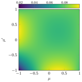
We would like to point out that the previous Assumption 3.3 is necessary to get rid of the drift terms in Equation (18). Even though many kernels satisfying Assumption 2.1 also satisfy Assumption 3.3, this is not true in general, see, e.g.,
| (20) |
which yields for the matrix
A plot of this kernel (projected onto the -component) is given in Figure 1. However, numerical tests (checkKernelAssumption.m) have shown that many physically relevant kernels do satisfy this assumption (without proof), like linearly anisotropic scattering (Eddington scattering), Rayleigh scattering, Kagiwada-Kalaba scattering or the von-Mises-Fischer scattering [60, 61, 62, 63]. Especially those kernels satisfying the assumption in Lemma Lemma 3.5 have the desired property.
Lemma 3.5 (No drift).
Proof.
We only show the result for even, i.e., . The case of odd works analogously. The final result then follows by considering the even-odd decomposition of the general kernel as , where and denote the even and odd parts of , respectively.
Let be any rotation matrix that rotates to , i.e., with . We define the new parametrization of as . Due to the choice of our angular basis it can be shown [32, 8] that there is a rotation matrix with
respectively for the vector of even basis functions. Then we have by the substitution rule that
We now only consider the inner integral:
where we used that the and are periodic in the last equality. Thus, as well. The proof works in the same way for odd kernels, where we define the rotation matrix such that , and , and only consider the integral with respect to . ∎
We now want to show that the reduction operator (17) is well-defined.
Lemma 3.6 (Solving for in Equation (16b)).
Let the kernel satisfy Assumption 2.1. The matrix is invertible whenever .
Proof.
We have that
especially is symmetric due to the symmetry of . Let and we define , then it holds:
where we used that
| (21) |
as every entry in is orthogonal to and thus to all constants w.r.t. , and
| (22) |
In particular, since and , we get that , which implies that is negative definite and therefore invertible. ∎
3.2 Weak formulation and boundary conditions
One major problem of the equations is that the boundary conditions (4) of the transfer equation have to be prescribed for inward-pointing angles () only, whereas the hyperbolic system requires information for the characteristic variables related to ingoing characteristics [64]. Although these quantities are somehow related, a consistent approximation of boundary conditions for moment models is non-trivial [65, 66, 67, 68, 69].
Without thinking too much about these implications for the equations, we want to use the Marshak approach to derive consistent boundary conditions for Equation (18). The basic idea is to replace in Equation (4) with the ansatz and take half moments over of the equation w.r.t. to a suitable subset of basis functions. Using all basis functions would provide more boundary conditions than actually needed. The choice of “all relevant” basis functions is also discussed in [9]. We choose all odd basis functions in for the half moments at the boundary as those are the ones which appear naturally in the weak formulation as discussed below. This also leads to more equations than unknowns but guarantees the existence of the second-order formulation as shown in Lemma 3.7. Whereas we reason with the existence of our second-order formulation for this particular choice of basis functions, this choice was already taken before in literature, e.g., in a classical context in [70].
We start to derive the weak form for . Let denote a suitable spatial test function and . The weak form then reads
| (23) | ||||
where we used the divergence theorem in the last step. We now want to eliminate in Equation (LABEL:eq:weakform1) using the boundary conditions. Therefore we consider half moments of Equation (4) with respect to the odd basis functions:
| (24) |
We note that might depend on the position as well as the orientation of the boundary, i.e., the unit outer normal vector . Plugging in the definition of the ansatz (15) yields
Defining the matrices
| (25a) | ||||
| (25b) | ||||
we are able to rewrite the equation above, given that the matrix is invertible (see Lemma 3.7), as
| (26) |
Thus, the final weak form reads
| (27) | ||||
It remains to show, that the reduction (26) is well-defined.
Lemma 3.7 (Solving for in Equation (26)).
The matrix is invertible for all .
Proof.
The rotation matrix that rotates a vector around the axis by an angle of is given by
The reflection of at the plane can be represented by a rotation around by an angle of and a subsequent negation:
Like in the proof of Lemma 3.5 there is a rotation matrix , only depending on , with
Using the parity of the odd real spherical harmonics, i.e., , and our assumption, that the reflectivity does not depend on , we can rewrite the matrix as
is thus invertible if and are invertible. Consider the vector . Then we have that
since and the real spherical harmonics being linearly independent and continuous. Thus, the first matrix in the product is symmetric, positive definite and thus invertible. Using a Neumann series, is invertible if for any matrix norm. In particular, since is a rotation matrix, it has (induced operator norm), such that we get if .
Remark 3.8.
Lemma 3.7 proves the invertibility of the matrix for , which especially includes our case .
Remark 3.9.
Due to parity and the fact that , we get that and .
4 Numerical Results
The different test cases demonstrate the broad applicability of our approach to different scenarios including heterogeneous coefficients, anisotropic scattering, anisotropic boundary sources and different spatial dimensions. We reduced the computational complexity by looking at reduced problems in one and two space dimensions like described in Section 2.2, whereas we provide code for the full 3D scenario as well.
4.1 Code interface / Implementation details
Our Matlab code for the evaluation of the real spherical harmonics is based on [32]. We would like to note here that our implementation does not include the Condon-Shortley phase (“ prefactor”) in contrary to, e.g., Matlab’s legendre function. The (permuted version of the) flux matrices are given explicitly in [4]. We approximate the integrals over (subdomains of) the unit sphere by a quadrature rule. This is based on a trigonometric Gaussian quadrature rule for polynomials on a circle, described, e.g., in [71]. We employ the authors implementation of this quadrature rule in Matlab, provided in [72]. For a detailed investigation in the reduced 2D case, see [30].
In cases for which we do not know the reference solution of the kinetic problem or the original equations, we compare our result to the approximate solution of the discrete ordinates method. For a recent survey and relevant references, see [73]. For our implementation of the discrete ordinates method in 2D we needed barycentric interpolation on the sphere like described in [74].
We discretize the weak formulation of the systems using linear Lagrange finite elements with the help of FEniCS.
4.2 Test case 1
The first test case is rather simple and we are able to compute analytic reference solutions for the kinetic problem and the original equations, which allows us to validate our code in this setup, which is given in Table 3.
| = | |||
It is easy to check that the analytic reference solution for the kinetic problem is given by
| (28) | ||||
| (29) |
In this simple case we can reformulate the system as an initial value problem. This gives us up to the precision of the solution of the corresponding ODE a reference solution, denoted by , for the solutions of the approach.
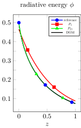
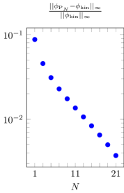
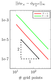
In Figure 2 we present the results of a numerical study of this test case, where we compare different approximations of the radiative energy with the analytic reference solution, see Subfigure 2(a). For the discrete ordinates method we use a quadrature rule on the unit sphere which is exact for polynomials up to degree 23 and obtain 50 discrete ordinates after reduction to 1D (by fixing and only discretizing ). Furthermore we look at the convergence of the radiative energies of the solutions to the one of the kinetic reference solution for increasing moment order , see Subfigure 2(b), and the convergence of the radiative energies of the numerical approximations of the equations to the ones of the reference solutions, see Subfigure 2(c).
From the analytic solution of the kinetic problem (28) we see that we would need infinitely many real spherical harmonics in the basis expansion to describe the true solution, which gives reason for the slow convergence.
This test case indicates the convergence of the solutions of the method to the true solution of the kinetic problem and furthermore the equivalence of the solutions of the original equations and our second-order formulation (in cases where the derivation is justified).
Referring to our repository on GitHub [22], we list the functions used to compute the different approximations of the distribution and radiative energy in Table 4.
| wrapper | runTestCase1.m | |
| kinetic reference solution | radiativeEnergyKineticSolutionTestCase1.m | |
| discrete ordinates method | mainDiscreteOrdinates1D.m | |
| reference solution | radiativeEnergyPNOrigIsotropicKernel1D.m | |
| solution | runTestCase1.py | |
| transformation | generateTestCase1.m |
4.3 Test case 2
The second test case demonstrates that we are able to treat heterogeneous coefficients, non-vanishing reflectivity at the boundary and anisotropic boundary sources in 1D. The setup for this test case in 1D is given in Table 5.
For this test case we are again able to compute a reference solution of the original system by reformulating this as initial value problem.
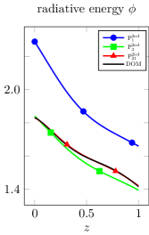
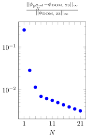
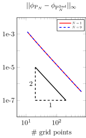
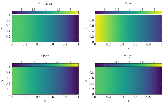
In Figure 3 we present the results of a numerical study of this test case, where we compare different approximations of the radiative energy with the approximation by the discrete ordinates method as reference solution, see Subfigure 3(a). For the discrete ordinates method we used a quadrature rule on the unit sphere which is exact for polynomials up to degree 23 and obtain 50 ordinates after reduction to 1D (by fixing and only discretizing ). Furthermore we look at the convergence of the radiative energies of the solutions to the one of the discrete ordinates method for increasing moment order , see Subfigure 3(b), and the convergence of the radiative energies of the numerical approximations of the equations to the ones of the reference solutions, see Subfigure 3(c).
We observe a significant jump already between the first two moment orders.
Referring to our repository on GitHub [22], we list the functions used to compute the different approximations of the distribution and radiative energy in Table 6.
| wrapper | runTestCase2.m | |
| discrete ordinates method | mainDiscreteOrdinates1D.m | |
| reference solution | radiativeEnergyPNOrigIsotropicKernel1D.m | |
| solution | runTestCase2.py | |
| transformation | generateTestCase2.m |
4.4 Test case 3
The third test case demonstrates that our method is not limited to isotropic scattering. The setup for this test case in 1D is given in Table 7.
| = | |||
We are able to compute an analytic reference solution for the kinetic problem, which reads:
| (45) |
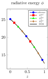
We see that the analytic solution is a first-order polynomial in , thus we expect that the solution of the equations should give the exact solution of the kinetic problem.
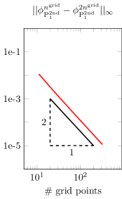
In Figure 4 we present the results of a numerical study of this test case, where we compare different approximations of the radiative energy with the analytic reference solution, see Subfigure 4(a). For the discrete ordinates method we use a quadrature rule on the unit sphere which is exact for polynomials up to degree 23, where we did not reduce the set of ordinates in this case and ended up with 600 discrete ordinates on the full sphere. Furthermore we look at the convergence of the radiative energies of the numerical approximations of the by comparing the solution on a certain grid to the one on a refined grid, see Subfigure 4(b).
Referring to our repository on GitHub [22], we list the functions used to compute the different approximations of the distribution and radiative energy in Table 8.
| wrapper | runTestCase3.m | |
| kinetic reference solution | radiativeEnergyKineticSolutionTestCase3.m | |
| discrete ordinates method | mainDiscreteOrdinates1D.m | |
| solution | runTestCase3.py | |
| transformation | generateTestCase3.m |
4.5 Test case 4
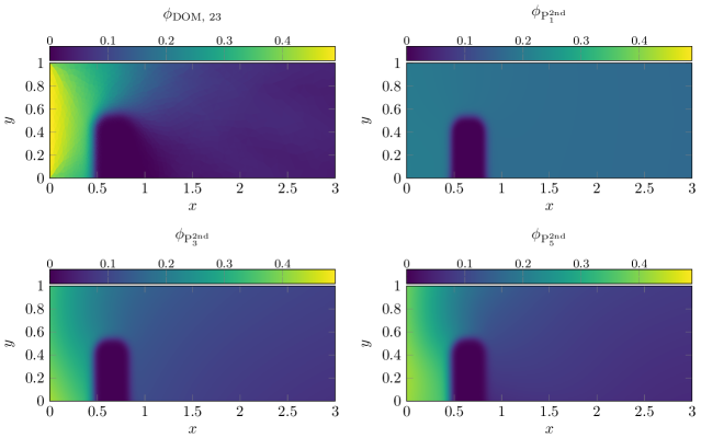
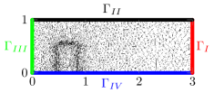
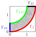
This test case demonstrates that our method can deal with heterogeneous coefficients in 2D. It is based on the shadow test [39, 50] which represents a particle stream that is partially blocked by an absorber, resulting in a shadowed region behind the absorber. The setup for this test case in 2D is given in Table 9, based on the auxiliary functions in Equation (51). The domain and the partition of the boundary are illustrated in Figure 6(a).
| (51a) | ||||
| (51b) | ||||
| (51c) | ||||
| = | = | = | = |
| = | = | = | = |
For the spatial discretization we use a triangular mesh with 2699 nodes and 5252 elements. We refine the mesh by splitting [78] and obtain a mesh with 10649 nodes and 21008 elements for numerical reference solutions of the corresponding models, denoted by . As reference we compute the discrete ordinates solution on the coarse mesh. As before we use for the discretization of the unit sphere a Gaussian-like quadrature rule which is exact for polynomials up to degree 23 and leaves us with 600 ordinates on the upper half sphere after reduction to 2D. We compare this solution to the discrete ordinates solution with a quadrature rule exact up to degree 15 with 272 ordinates on the upper half sphere.
In Figure 5 we show the radiative energies of the discrete ordinates solution and the solutions. In Table 11 we show the relative distances of the radiative energies of the solutions on the coarse grid to the corresponding reference solutions on the refined grid and the discrete ordinates solution.
We see that the distance of the radiative energies of the solutions to the discrete ordinate solutions decreases, but it seems that a much larger moment order would be necessary to get a satisfying approximation. Furthermore we would like to note that the presented discrete ordinates solution is only to a certain extent suitable as a reference solution, as its relative distance to the solution with around half as many discrete ordinates is about 4%.
Referring to our repository on GitHub [22], we list the functions used to compute the different approximations of the distribution and radiative energy in Table 10.
| wrapper | runTestCase4.m | |
| mesh generation and refinement | genMeshTestCase4.sh | |
| discrete ordinates method | runDiscreteOrdinatesTestCase4.m | |
| solution | runTestCase4.py | |
| transformation | generateTestCase4.m |
| 1 | 2.03e-03 | 7.18e-01 |
| 3 | 2.39e-03 | 3.41e-01 |
| 5 | 1.01e-02 | 2.47e-01 |
| 7 | 1.40e-02 | 1.91e-01 |
4.6 Test case 5
The fifth test case considers the popular Henyey Greenstein scattering kernel. This especially demonstrates that our method is not limited to isotropic scattering. For the spatial discretization we use a triangular mesh with 2212 nodes and 4262 elements. We refine the mesh by splitting [78] and obtain a mesh with 8685 nodes and 17048 elements for numerical reference solutions of the corresponding models, denoted by . As reference we compute the discrete ordinates solution on the coarse mesh. As before we use for the discretization of the unit sphere a Gaussian-like quadrature rule which is exact for polynomials up to degree 23 and leaves us with 600 ordinates on the full unit sphere. We compare this solution to the discrete ordinates solution with a quadrature rule exact up to degree 15 with 272 ordinates on the full unit sphere.
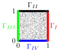
The setup for this test case in 2D is given in Table 12. The domain and the partition of the boundary are illustrated in Figure 6(b). We choose the anisotropy factor in the Henyey-Greenstein kernel .
| = | |||
| = | = | = | = |
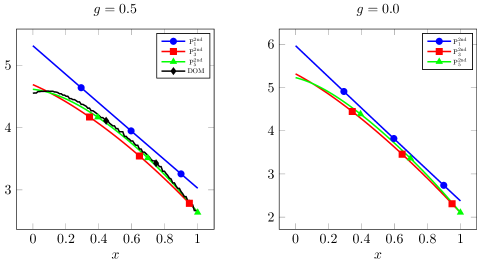
In Figure 7 we show the radiative energies of the discrete ordinates solution and the solutions. In Figure 8 we compare the radiative energies for different model orders and the anisotropy factors and along the line . We would like to note, that reproduces anisotropic scattering. The non-smootheness in the line plot of the discrete ordinates solution is caused by interpolation of the corresponding piecewise constant function w.r.t. the elements. In Table 14 we show the relative distances of the radiative energies of the solutions on the coarse grid to the corresponding reference solutions on the refined grid and the discrete ordinates solution.
Referring to our repository on GitHub [22], we list the functions used to compute the different approximations of the distribution and radiative energy in Table 13.
| wrapper | runTestCase5.m | |
| mesh generation and refinement | genMeshTestCase5.sh | |
| discrete ordinates method | runDiscreteOrdinatesTestCase5.m | |
| solution | runTestCase5.py | |
| transformation | generateTestCase5.m |
| 1 | 3.55e-07 | 8.07e-02 |
| 3 | 1.75e-05 | 2.73e-02 |
| 5 | 4.12e-05 | 1.02e-02 |
| 7 | 7.26e-05 | 4.03e-03 |
4.7 Test case 6
This test case demonstrates that our method is not limited to rectangular domains and especially can be used with irregular grids.
For the spatial discretization we use a triangular mesh with 2530 nodes and 4847 elements. We refine the mesh by splitting [78] and obtain a mesh with 9906 nodes and 19388 elements for numerical reference solutions of the corresponding models, denoted by . As reference we compute the discrete ordinates solution on the coarse mesh. As before we use for the discretization of the unit sphere a Gaussian-like quadrature rule which is exact for polynomials up to degree 23 and leaves us with 600 ordinates on the upper half sphere. We compare this solution to the discrete ordinates solution with a quadrature rule exact up to degree 15 with 272 ordinates on the upper half sphere.
The setup for this test case in 2D is given in Table 15. The domain and the partition of the boundary is illustrated in Figure 6(c).
| : see Figure 6(c) | |||
| = | = | = | = |
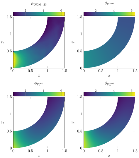
In Figure 9 we show the radiative energies of the discrete ordinates solution and the solutions. In Table 17 we show the relative distances of the radiative energies of the solutions on the coarse grid to the corresponding reference solutions on the refined grid and the discrete ordinates solution.
Referring to our repository on GitHub [22], we list the functions used to compute the different approximations of the distribution and radiative energy in Table 16.
| wrapper | runTestCase6.m | |
| mesh generation and refinement | genMeshTestCase6.sh | |
| discrete ordinates method | runDiscreteOrdinatesTestCase6.m | |
| solution | runTestCase6.py | |
| transformation | generateTestCase6.m |
| 1 | 1.00e-05 | 3.34e-01 |
| 3 | 3.77e-04 | 1.43e-01 |
| 5 | 1.08e-03 | 9.53e-02 |
| 7 | 4.00e-03 | 8.48e-02 |
5 Conclusion
We presented the second-order formulation of the classical equations for the monoenergetic stationary linear transport equation. In contrary to classical approaches, we reproduce the even moments of the original system.
We approximate the semi-transparent boundary conditions on the kinetic level by taking half moments at the boundary and obtain Marshak boundary conditions. Taking half moments at the boundary w.r.t. all real spherical harmonics up to the used order would yield too many boundary conditions, where our derivation suggests the “natural” selection of a subset of those real spherical harmonics based on the weak formulation.
The algebraic transformations can be handed to a computer algebra system and the solution of the resulting weak formulation can be delegated to established PDE tools. We demonstrated this workflow with Matlab’s symbolic toolbox and FEniCS. Our implementation is not necessarily designed to yield a high performance solution scheme, in fact it should be seen as a proof of concept and easy-to-use tool for fast prototyping.
We demonstrated in six numerical test cases the flexibility and wide applicability of our approach.
Our derivation is based on the assumption, that all algebraic elimination steps are justified. Especially we assume that the solution of the original system is of certain regularity and that all (higher order) derivatives are well defined. We proved, under these regularity assumptions on the solutions and mild additional assumptions in Lemmas 3.5, 3.6 and 3.7, that the resulting second-order formulation is well defined. It would be an interesting task for the future to investigate the well-posedness of the resulting system.
Acknowledgement
The authors are grateful for the support of the German Federal Ministry of Education and Research (BMBF) grant no. 05M16UKE.
References
References
-
[1]
F. Hübner, C. Leithäuser, B. Bazrafshan, N. Siedow, T. J. Vogl,
Validation of a mathematical
model for laser-induced thermotherapy in liver tissue, Lasers in Medical
Science 32 (6) (2017) 1399–1409.
doi:10.1007/s10103-017-2260-4.
URL https://doi.org/10.1007/s10103-017-2260-4 - [2] R. Pinnau, G. Thömmes, Optimal boundary control of glass cooling processes, Mathematical methods in the applied sciences 27 (11) (2004) 1261–1281.
- [3] T. A. Brunner, Forms of approximate radiation transport, Sandia report.
-
[4]
B. Seibold, M. Frank, Starmap—a
second order staggered grid method for spherical harmonics moment equations
of radiative transfer, ACM Transactions on Mathematical Software 41 (1)
(2014) 4:1–4:28.
doi:10.1145/2590808.
URL http://doi.acm.org/10.1145/2590808 - [5] W. Ge, R. Marquez, M. F. Modest, S. P. Roy, Implementation of high-order spherical harmonics methods for radiative heat transfer on openfoam, Journal of Heat Transfer 137 (5) (2015) 052701.
-
[6]
J. T. Tencer,
Error analysis
for radiation transport, dissertation, The University of Texas at Austin
(2013).
URL https://repositories.lib.utexas.edu/handle/2152/23247 -
[7]
R. G. McClarren,
Theoretical aspects of
the simplified equations, Transport Theory and Statistical Physics
39 (2-4) (2010) 73–109.
doi:10.1080/00411450.2010.535088.
URL https://doi.org/10.1080/00411450.2010.535088 -
[8]
M. F. Modest, J. Yang,
Elliptic
pde formulation and boundary conditions of the spherical harmonics method of
arbitrary order for general three-dimensional geometries, Journal of
Quantitative Spectroscopy and Radiative Transfer 109 (9) (2008) 1641 – 1666.
doi:https://doi.org/10.1016/j.jqsrt.2007.12.018.
URL http://www.sciencedirect.com/science/article/pii/S0022407307003676 -
[9]
M. F. Modest, Further
development of the elliptic pde formulation of the p n approximation and its
marshak boundary conditions, Numerical Heat Transfer, Part B: Fundamentals
62 (2-3) (2012) 181–202.
doi:10.1080/10407790.2012.702645.
URL https://doi.org/10.1080/10407790.2012.702645 - [10] W. Ge, High-order spherical harmonics methods for radiative heat transfer and applications in combustion simulations, Ph.D. thesis, UC Merced (2017).
-
[11]
A. D. Klose, E. W. Larsen,
Light
transport in biological tissue based on the simplified spherical harmonics
equations, Journal of Computational Physics 220 (1) (2006) 441 – 470.
doi:https://doi.org/10.1016/j.jcp.2006.07.007.
URL http://www.sciencedirect.com/science/article/pii/S0021999106003421 -
[12]
S. P. Hamilton, T. M. Evans,
Efficient
solution of the simplified equations, Journal of Computational
Physics 284 (2015) 155 – 170.
doi:https://doi.org/10.1016/j.jcp.2014.12.014.
URL http://www.sciencedirect.com/science/article/pii/S0021999114008225 -
[13]
M. F. Modest, J. Cai, W. Ge, E. Lee,
Elliptic
formulation of the simplified spherical harmonics method in radiative heat
transfer, International Journal of Heat and Mass Transfer 76 (2014) 459 –
466.
doi:https://doi.org/10.1016/j.ijheatmasstransfer.2014.04.038.
URL http://www.sciencedirect.com/science/article/pii/S0017931014003433 -
[14]
Y. Zhang, J. C. Ragusa, J. E. Morel,
Iterative
performance of various formulations of the s equations, Journal of
Computational Physics 252 (2013) 558 – 572.
doi:https://doi.org/10.1016/j.jcp.2013.06.009.
URL http://www.sciencedirect.com/science/article/pii/S0021999113004336 -
[15]
K. Liu, Y. Lu, J. Tian, C. Qin, X. Yang, S. Zhu, X. Yang, Q. Gao, D. Han,
Evaluation
of the simplified spherical harmonics approximation in bioluminescence
tomography through heterogeneous mouse models, Opt. Express 18 (20) (2010)
20988–21002.
doi:10.1364/OE.18.020988.
URL http://www.opticsexpress.org/abstract.cfm?URI=oe-18-20-20988 -
[16]
C. Pu, R. G. McClarren,
Mathematical and
numerical validation of the simplified spherical harmonics approach for
time-dependent anisotropic-scattering transport problems in homogeneous
media, Journal of Computational and Theoretical Transport 46 (5) (2017)
366–378.
doi:10.1080/23324309.2017.1352516.
URL https://doi.org/10.1080/23324309.2017.1352516 -
[17]
MATLAB, Matlab and symbolic toolbox release
2018b (2018).
URL https://de.mathworks.com/ -
[18]
M. Alnæs, J. Blechta, J. Hake, A. Johansson, B. Kehlet, A. Logg,
C. Richardson, J. Ring, M. E. Rognes, G. N. Wells,
The fenics project version 1.5, Archive of
Numerical Software 3 (100) (2015) 9–23.
URL https://fenicsproject.org/ - [19] A. Logg, K.-A. Mardal, G. Wells, Automated Solution of Differential Equations by the Finite Element Method: The FEniCS Book, Vol. 84, Springer Science & Business Media, 2012.
- [20] R. J. LeVeque, Python tools for reproducible research on hyperbolic problems, Computing in Science Engineering 11 (1) (2009) 19–27. doi:10.1109/MCSE.2009.13.
- [21] M. D. Wilkinson, M. Dumontier, I. J. Aalbersberg, G. Appleton, M. Axton, A. Baak, N. Blomberg, J.-W. Boiten, L. B. da Silva Santos, P. E. Bourne, et al., The fair guiding principles for scientific data management and stewardship, Scientific data 3.
- [22] M. Andres, F. Schneider, Github repository for this project, https://github.com/andresmatthias/pn2nd.git, contains MATLAB and Python codes related to this article to reproduce the numerical results. Accessed: 2019-08-01.
-
[23]
C. Cercignani, The
Boltzmann Equation and its Applications, Applied mathematical sciences ; 67,
Springer, Berlin u.a., 1988.
URL https://kplus.ub.uni-kl.de/Record/KLU01-000183612 -
[24]
S. J. Park, S.-B. Yun,
Entropy
production estimates for the polyatomic ellipsoidal bgk model, Applied
Mathematics Letters 58 (2016) 26 – 33.
doi:https://doi.org/10.1016/j.aml.2016.01.021.
URL http://www.sciencedirect.com/science/article/pii/S089396591630043X -
[25]
C. D. Levermore, Moment closure
hierarchies for kinetic theories, Journal of Statistical Physics 83 (5)
(1996) 1021–1065.
doi:10.1007/BF02179552.
URL https://doi.org/10.1007/BF02179552 - [26] L. G. Henyey, J. L. Greenstein, Diffuse radiation in the galaxy, Astrophysical Journal 93 (1941) 70–83. doi:10.1086/144246.
-
[27]
E. W. Larsen, G. Thömmes, A. Klar, M. Seaïd, T. Götz,
Simplified
approximations to the equations of radiative heat transfer and
applications, Journal of Computational Physics 183 (2) (2002) 652 – 675.
doi:https://doi.org/10.1006/jcph.2002.7210.
URL http://www.sciencedirect.com/science/article/pii/S0021999102972104 -
[28]
E. Olbrant, M. Frank,
Generalized fokker-planck
theory for electron and photon transport in biological tissues: Application
to radiotherapy, Computational and mathematical methods in medicine 11 (4)
(2010) 313–39.
doi:10.1080/1748670X.2010.491828.
URL http://www.ncbi.nlm.nih.gov/pubmed/20924856 -
[29]
B. Dubroca, J.-L. Feugeas, M. Frank,
Angular
moment model for the fokker-planck equation, The European Physical Journal D
60 (2) (2010) 301–307.
doi:10.1140/epjd/e2010-00190-8.
URL http://www.springerlink.com/index/10.1140/epjd/e2010-00190-8 -
[30]
F. Schneider, Moment
models in radiation transport equations, Ph.D. thesis, TU Kaiserslautern,
München (2016).
URL https://kplus.ub.uni-kl.de/Record/KLU01-001010407 -
[31]
T. A. Brunner, J. P. Holloway,
Two-dimensional
time dependent riemann solvers for neutron transport, Journal of
Computational Physics 210 (1) (2005) 386 – 399.
doi:https://doi.org/10.1016/j.jcp.2005.04.011.
URL http://www.sciencedirect.com/science/article/pii/S0021999105002275 -
[32]
M. A. Blanco, M. Flórez, M. Bermejo,
Evaluation
of the rotation matrices in the basis of real spherical harmonics, Journal
of Molecular Structure: THEOCHEM 419 (1) (1997) 19 – 27.
doi:https://doi.org/10.1016/S0166-1280(97)00185-1.
URL http://www.sciencedirect.com/science/article/pii/S0166128097001851 -
[33]
R. Courant, D. Hilbert,
Methods
of Mathematical Physics, no. Bd. 1 in Methods of Mathematical Physics,
Wiley, 2008.
URL https://archive.org/details/MethodsOfMathematicalPhysicsVolume1 - [34] A. S. Eddington, The Internal Constitution of the Stars, Dover, 1926.
- [35] E. E. Lewis, J. W. F. Miller, Computational Methods in Neutron Transport, John Wiley and Sons, New York, 1984.
-
[36]
E. Tadmor,
Approximate
Solutions of Nonlinear Conservation Laws, Springer, 1998.
URL http://link.springer.com/chapter/10.1007/BFb0096352 -
[37]
C.-W. Shu,
Essentially
Non-Oscillatory and Weighted Essentially Non-Oscillatory Schemes for
Hyperbolic Conservation Laws, Springer, 1998.
URL http://link.springer.com/chapter/10.1007/BFb0096355 -
[38]
C. K. Garrett, C. D. Hauck,
A
comparison of moment closures for linear kinetic transport equations: The
line source benchmark, Transport Theory and Statistical Physics.
URL http://www.tandfonline.com/doi/abs/10.1080/00411450.2014.910226 -
[39]
P. Chidyagwai, M. Frank, F. Schneider, B. Seibold,
A
comparative study of limiting strategies in discontinuous galerkin schemes
for the m1 model of radiation transport, Journal of Computational and
Applied Mathematics 342 (2018) 399 – 418.
doi:https://doi.org/10.1016/j.cam.2018.04.017.
URL http://www.sciencedirect.com/science/article/pii/S0377042718301857 -
[40]
C. D. Levermore,
Relating
eddington factors to flux limiters, Journal of Quantitative Spectroscopy and
Radiative … 31 (2) (1984) 149–160.
URL http://www.sciencedirect.com/science/article/pii/0022407384901122 -
[41]
L. R. Mead, N. Papanicolaou,
Maximum
entropy in the problem of moments, Journal of Mathematical Physics 25 (8)
(1984) 2404.
doi:10.1063/1.526446.
URL http://link.aip.org/link/JMAPAQ/v25/i8/p2404/s1{&}Agg=doi -
[42]
J. Cernohorsky, S. Bludman,
Maximum entropy
distribution and closure for bose-einstein and fermi-dirac radiation
transport, The Astrophysical Journal.
URL http://adsabs.harvard.edu/full/1994ApJ...433..250C - [43] B. Dubroca, J.-L. Feugeas, Entropic moment closure hierarchy for the radiative transfer equation, C. R. Acad. Sci. Paris Ser. I 329 (1999) 915–920.
- [44] M. Junk, Maximum entropy for reduced moment problems, Math. Meth. Mod. Appl. Sci. 10 (2000) 1001–1025.
- [45] G. N. Minerbo, Maximum entropy eddington factors, J. Quant. Spectrosc. Radiat. Transfer 20 (1978) 541–545.
-
[46]
T. A. Brunner, J. P. Holloway,
One-dimensional
riemann solvers and the maximum entropy closure, Journal of Quantitative
Spectroscopy and Radiative Transfer 69 (5) (2001) 543–566.
doi:10.1016/S0022-4073(00)00099-6.
URL http://www.sciencedirect.com/science/article/pii/S0022407300000996http://linkinghub.elsevier.com/retrieve/pii/S0022407300000996 -
[47]
E. Olbrant, C. D. Hauck, M. Frank,
A
realizability-preserving discontinuous galerkin method for the m1 model of
radiative transfer, Journal of Computational Physics 231 (17) (2012)
5612–5639.
doi:10.1016/j.jcp.2012.03.002.
URL http://linkinghub.elsevier.com/retrieve/pii/S0021999112001362 -
[48]
C. D. Hauck,
High-order
entropy-based closures for linear transport in slab geometry, Commun. Math.
Sci. v9.
URL http://www.ki-net.umd.edu/pubs/files/FRG-2010-Hauck-Cory.entropy{_}kinetic.pdf -
[49]
G. W. Alldredge, C. D. Hauck, A. L. Tits,
High-order
entropy-based closures for linear transport in slab geometry ii: A
computational study of the optimization problem, SIAM Journal on Scientific
Computing 34 (4) (2012) B361–B391.
doi:10.1137/11084772X.
URL http://epubs.siam.org/doi/abs/10.1137/11084772X - [50] F. Schneider, T. Leibner, First-order continuous- and discontinuous-galerkin moment models for a linear kinetic equation: Realizability-preserving splitting scheme and numerical analysis (2019). arXiv:1904.03098.
-
[51]
M. Frank, B. Dubroca, A. Klar,
Partial
moment entropy approximation to radiative heat transfer, Journal of
Computational Physics 218 (1) (2006) 1–18.
URL http://www.sciencedirect.com/science/article/pii/S002199910600057X -
[52]
B. Dubroca, A. Klar,
Half-moment
closure for radiative transfer equations, Journal of Computational Physics
180 (2002) 584–596.
URL http://www.sciencedirect.com/science/article/pii/S0021999102971068 -
[53]
F. Schneider, G. W. Alldredge, M. Frank, A. Klar,
Higher order
mixed-moment approximations for the fokker–planck equation in one space
dimension, SIAM Journal on Applied Mathematics 74 (4) (2014) 1087–1114.
arXiv:1405.5305,
doi:10.1137/130934210.
URL http://epubs.siam.org/doi/abs/10.1137/130934210 -
[54]
J. Ritter, A. Klar, F. Schneider,
Partial-moment minimum-entropy models
for kinetic chemotaxis equations in one and two dimensions, Journal of
Computational and Applied Mathematics 306 (2016) 300–315.
arXiv:1601.04482,
doi:10.1016/j.cam.2016.04.019.
URL http://arxiv.org/abs/1601.04482 -
[55]
F. Schneider, J. Kall, A. Roth,
First-order
quarter- and mixed-moment realizability theory and kershaw closures for a
fokker-planck equation in two space dimensions, Kinetic and Related Models
10.
doi:10.3934/krm.2017044.
URL http://aimsciences.org//article/id/92206f8c-b216-478b-a566-d72a803c8ab9 -
[56]
D. S. Kershaw,
Flux
limiting nature’s own way: A new method for numerical solution of the
transport equation, Tech. rep., LLNL Report UCRL-78378 (jul 1976).
doi:10.2172/104974.
URL http://www.osti.gov/bridge/product.biblio.jsp?osti{_}id=104974 - [57] P. Monreal, Moment realizability and kershaw closures in radiative transfer, Ph.D. thesis, TU Aachen (2012).
-
[58]
F. Schneider, Kershaw closures for
linear transport equations in slab geometry i: Model derivation, Journal of
Computational Physics 322 (2016) 905–919.
arXiv:1511.02714,
doi:10.1016/j.jcp.2016.02.080.
URL http://arxiv.org/abs/1511.02714 -
[59]
F. Schneider, Kershaw closures for
linear transport equations in slab geometry ii: high-order
realizability-preserving discontinuous-galerkin schemes, Journal of
Computational Physics 322 (2016) 920–935.
arXiv:1602.02590,
doi:10.1016/j.jcp.2016.07.014.
URL http://arxiv.org/abs/1602.02590 -
[60]
E. d’Eon, A hitchhiker’s guide to
multiple scattering, Tech. rep., Technical report (2016).
URL http://www.eugenedeon.com/hitchhikers - [61] S. Chandrasekhar, Radiative Transfer, Courier Corporation, 2013.
- [62] H. Kagiwada, R. Kalaba, Multiple anisotropic scattering in slabs with axially symmetric fields, Tech. rep., RAND CORP SANTA MONICA CALIF (1967).
-
[63]
I. Gkioulekas, B. Xiao, S. Zhao, E. H. Adelson, T. Zickler, K. Bala,
Understanding the role of
phase function in translucent appearance, ACM Trans. Graph. 32 (5) (2013)
147:1–147:19.
doi:10.1145/2516971.2516972.
URL http://doi.acm.org/10.1145/2516971.2516972 -
[64]
E. F. Toro, Riemann
Solvers and Numerical Methods for Fluid Dynamics, 3rd Edition, Springer,
Dordrecht u.a., 2009.
URL https://kplus.ub.uni-kl.de/Record/KLU01-000747419 -
[65]
G. C. Pomraning,
Variational
boundary conditions for the spherical harmonics approximation to the neutron
transport equation, Annals of Physics 27 (2) (1964) 193 – 215.
doi:https://doi.org/10.1016/0003-4916(64)90105-8.
URL http://www.sciencedirect.com/science/article/pii/0003491664901058 -
[66]
E. W. Larsen, G. C. Pomraning, The PN
Theory as an Asymptotic Limit of Transport Theory in Planar Geometry —I:
Analysis, Nuclear Science and Engineering 109 (1) (1991) 49–75.
URL http://epubs.ans.org/?a=23844 -
[67]
R. P. Rulko, E. W. Larsen, G. C. Pomraning,
The PN Theory as an Asymptotic Limit of
Transport Theory in Planar Geometry —II: Numerical Results, Nuclear
Science and Engineering 109 (1) (1991) 76–85.
URL http://epubs.ans.org/?a=23845 -
[68]
H. Struchtrup, Kinetic
schemes and boundary conditions for moment equations, Zeitschrift für
angewandte Mathematik und Physik 51 (3) (2000) 346.
doi:10.1007/s000330050002.
URL http://link.springer.com/10.1007/s000330050002 - [69] C. D. Levermore, Boundary conditions for moment closures, Institute for Pure and Applied Mathematics University of California, Los Angeles, CA on May 27.
-
[70]
S. P. Hamilton, T. M. Evans,
Efficient
solution of the simplified pn equations, Journal of Computational Physics
284 (2015) 155 – 170.
doi:https://doi.org/10.1016/j.jcp.2014.12.014.
URL http://www.sciencedirect.com/science/article/pii/S0021999114008225 - [71] G. Da Fies, M. Vianello, Trigonometric gaussian quadrature on subintervals of the period, Electronic Transactions on Numerical Analysis 39 (2012) 102–112.
- [72] G. Da Fies, A. Sommariva, V. M., Subp: Matlab package for subperiodic trigonometric quadrature and multivariate applications, https://www.math.unipd.it/~marcov/mysoft/subp/trigauss.m, contains codes for product Gaussian quadrature on circular and spherical sections.
- [73] E. W. Larsen, J. E. Morel, Advances in discrete-ordinates methodology, in: Nuclear Computational Science, Springer, 2010, pp. 1–84.
-
[74]
M. F. Carfora,
Interpolation
on spherical geodesic grids: A comparative study, Journal of Computational
and Applied Mathematics 210 (1) (2007) 99 – 105, proceedings of the
Numerical Analysis Conference 2005.
doi:https://doi.org/10.1016/j.cam.2006.10.068.
URL http://www.sciencedirect.com/science/article/pii/S0377042706006522 -
[75]
T. P. S. Foundation, Python.
URL https://www.python.org/ -
[76]
T. E. Oliphant, A Guide to NumPy, Vol. 1, Trelgol
Publishing USA, 2006.
URL https://numpy.org/ -
[77]
E. Jones, T. Oliphant, P. Peterson, et al.,
SciPy: Open source scientific tools for
Python (2001–).
URL http://www.scipy.org/ -
[78]
C. Geuzaine, J.-F. Remacle, Gmsh: a
three-dimensional finite element mesh generator with built-in pre- and
post-processing facilities, International Journal for Numerical Methods in
Engineering 79 (2009) 1309–1331.
URL http://www.gmsh.info/