Mean-field tricritical polymers

Abstract

We provide an introductory account of a tricritical phase diagram, in the setting of a mean-field random walk model of a polymer density transition, and clarify the nature of the density transition in this context. We consider a continuous-time random walk model on the complete graph, in the limit as the number of vertices $N$ in the graph grows to infinity. The walk has a repulsive self-interaction, as well as a competing attractive self-interaction whose strength is controlled by a parameter $g$. A chemical potential $\nu$ controls the walk length. We determine the phase diagram in the $(g,\nu)$ plane, as a model of a density transition for a single linear polymer chain. A dilute phase (walk of bounded length) is separated from a dense phase (walk of length of order $N$) by a phase boundary curve. The phase boundary is divided into two parts, corresponding to first-order and second-order phase transitions, with the division occurring at a tricritical point. The proof uses a supersymmetric representation for the random walk model, followed by a single block-spin renormalisation group step to reduce the problem to a 1-dimensional integral, followed by application of the Laplace method for an integral with a large parameter.

1 The model and results

1.1 Introduction

Models of critical phenomena such as the Ising model and percolation continue to be of central interest in the probability literature. In such models, a single parameter (temperature for the Ising model or occupation density for percolation) is tuned to a critical value in order to observe universal critical behaviour. In tricritical models, it is instead necessary to tune two parameters simultaneously to observe tricritical behaviour. Despite their importance for physical applications, tricritical phenomena have received much less attention in the mathematical literature than critical phenomena. Our purpose in this paper is to provide an introductory account of a tricritical phase diagram, in the setting of a mean-field random walk model of a polymer density transition, and to clarify the nature of the density transition in this context.

The self-avoiding walk is a starting point for the mathematical modelling of the chemical physics of a single linear polymer chain in a solvent [13]. The theory of the self-avoiding walk has primarily been developed in the setting of an infinite lattice, often ${\mathbb{Z}}^{d}$. So far, this theory has failed to provide theorems capturing the critical behaviour in dimensions $d=2,3$, such as a precise description of the typical end-to-end distance, and such problems are rightly considered to be both highly important and notoriously difficult. On ${\mathbb{Z}}^{d}$, basic quantities such as the susceptibility—the generating function $\sum_{n=0}^{\infty}c_{n}z^{n}$ for the number of $n$-step self-avoiding walks started from the origin—can be used to model a polymer chain in the dilute phase. The susceptibility is undefined when $|z|$ exceeds the reciprocal of the connective constant $\mu=\lim_{n\rightarrow\infty}c_{n}^{1/n}$. It is however large values of $z$ that are required to model the dense phase, as in [5, 17, 8], and some finite-volume approximation is needed for this. Much remains to be learned about the phase transition from the dilute to the dense phase, including its tricritical nature.

We study a mean-field model based on a continuous-time random walk on the complete graph on $N$ vertices, in the limit $N\rightarrow\infty$. The walk has a repulsive self-interaction which models the excluded-volume effect of a linear polymer, as well as a competing attractive self-interaction which models the tendency of the polymer to avoid contact with the solvent. The strength of the self-attraction is controlled by a parameter $g$, with attraction increasing as $g$ becomes more negative. A chemical potential $\nu$ controls the walk length. We investigate the phase diagram in the $(g,\nu)$ plane ${\mathbb{R}}^{2}$ (positive and negative values), as a model of a density transition for a single linear polymer chain.

Figure 1: Typical tricritical phase diagram. The second-order curve (dashed line) and the first-order curve (solid line) meet at the tricritical point. The shaded region is the dilute phase (bounded susceptibility) and the unshaded region is the dense phase.

In the physics literature, the nature of the phase diagram is well understood. The dilute and dense phases are separated by a phase boundary curve $\nu=\nu_{c}(g)$ as in Figure 1. The phase boundary itself is divided into two parts: a second-order part for $g>g_{c}$ across which the average polymer density varies continuously, and a first-order part for $g<g_{c}$ across which the density has a jump discontinuity. The two pieces of the phase boundary are separated by the tricritical point $(g_{c},\nu_{c}(g_{c}))$, known as the theta point. Tricritical behaviour differs from critical behaviour in the number of parameters that must be tuned. For critical behaviour, an experimentalist needs to tune a single variable to its critical value (given $g$, tune to $\nu_{c}(g)$). For tricritical behaviour, two variables must be tuned (tune to $(g_{c},\nu_{c}(g_{c}))$). A mathematically rigorous theory of the mean-field tricritical polymer density transition has been lacking, and our purpose here is to provide such a theory. Our analysis could be extended to study the tricritical behaviour of $n$-component spins or higher-order multi-critical points. Surprisingly, the mean-field theory of the density transition for the strictly self-avoiding walk has only very recently been developed [21, 7].

The upper critical dimension for the tricritical behaviour is predicted to be $d=3$, and mean-field tricritical behaviour is predicted for the model on ${\mathbb{Z}}^{d}$ in dimensions $d>3$. On the other hand, for the critical behaviour associated with the second-order part of the phase boundary, the upper critical dimension is instead $d=4$.

Nonrigorous methods were used in the physics literature to study the density transition in dimensions 2 and 3, and in particular its tricritical behaviour, in the 1980s [12, 9, 10, 11]. In recent work with Lohmann, we applied a rigorous renormalisation group method to study the 3-dimensional tricritical point [3], and proved that the tricritical two-point function has Gaussian $|x|^{-1}$ decay for the model on ${\mathbb{Z}}^{3}$. In [14], the transition across the second-order phase boundary was studied on a 4-dimensional hierarchical lattice, where a logarithmic correction to the mean-field behaviour of the density was proved. All of these references make use of an interpretation of the polymer model as the $n=0$ version of an $n$-component spin model. We also implement this strategy, using an exact representation of the random walk model based on supersymmetry. After a transformation which can be regarded as a single block-spin renormalisation group step, this representation takes on a form which permits application of the Laplace method for integrals involving a large parameter.

In the mathematical literature, it has been more common to model the polymer collapse transition in terms of the interacting self-avoiding walk in which a walk with a self-repulsion receives an energetic reward for nearest-neighbour contacts. A review of the literature on this model can be found in [16, Chapter 6]; more recent papers include [4, 15, 20]. In our mean-field model set on the complete graph, there is no geometry, and the notion of collapse (a highly localised walk) is not meaningful. We therefore concentrate on the density transition and its tricritical behaviour.

1.2 The model

1.2.1 Definitions

Let $\Lambda$ be a finite set with $N$ vertices; ultimately we are interested in the limit $N\rightarrow\infty$. Let $X=(X(t))_{t\in[0,\infty)}$ be the continuous-time simple random walk on the complete graph with vertex set $\Lambda$. This is the walk with generator $\Delta$ defined, for $f:\Lambda\rightarrow{\mathbb{R}}$, by

$$(\Delta f)_{x}=\frac{1}{N}\sum_{y\in\Lambda}(f_{y}-f_{x})\qquad(x\in\Lambda).$$ (1.1)

Equivalently, when the walk is at $x\in\Lambda$, it steps to a uniformly chosen vertex in $\Lambda\setminus\{x\}$ after an exponentially distributed holding time with rate $1-\frac{1}{N}$. The steps and holding times are all independent. We denote expectation for $X$ with initial point $X(0)=x$ by $E_{x}$.

The local time of $X$ at $x$ up to time $T$ is the random variable

$$L_{T,x}=\int_{0}^{T}\mathbbm{1}_{X(t)=x}\,dt\qquad(x\in\Lambda),$$ (1.2)

which measures the amount of time spent by the walk at $x$ up to time $T$. Let $L_{T}$ denote the vector of all local times. Given a function $p:[0,\infty)\rightarrow[0,\infty)$ with $p(0)=1$, we write $p_{N}(L_{T})=\prod_{x\in\Lambda}p(L_{T,x})$. Let $x,y\in\Lambda$. Assuming the integrals exist, the two-point function is

$$G_{xy}=\int_{0}^{\infty}E_{x}(p_{N}(L_{T})\mathbbm{1}_{X(T)=y})\,dT,$$ (1.3)

and the susceptibility is

$$\chi=\sum_{y\in\Lambda}G_{xy}=\int_{0}^{\infty}E_{x}(p_{N}(L_{T}))\,dT.$$ (1.4)

The right-hand side is independent of $x\in\Lambda$.

We define the random variable $L$, the length of $X$, by its probability density function

$$f_{L}(T)=\frac{1}{\chi}E_{x}\left(p_{N}(L_{T})\right)\qquad(T\geq 0),$$ (1.5)

which is also independent of $x\in\Lambda$. The expected value of the length is

$$\mathbb{E}L=\frac{1}{\chi}\int_{0}^{\infty}TE_{x}(p_{N}(L_{T}))\,dT.$$ (1.6)

The expected length can be written more compactly using a dot to represent differentiation with respect to $\epsilon$ at $\epsilon=0$, when $p(s)$ is replaced by $p(s)e^{-\epsilon s}$. With this notation, since $T=\sum_{x\in\Lambda}L_{T,x}$,

$$\mathbb{E}L=-\frac{1}{\chi}\dot{\chi}.$$ (1.7)

Assuming the limit exists, the density of the walk is defined by

$$\rho=\lim_{N\rightarrow\infty}\frac{1}{N}\mathbb{E}L.$$ (1.8)

1.2.2 Example

Although our results will be presented more generally, we are motivated by the example

$$p(t)=e^{-t^{3}-gt^{2}-\nu t}\qquad(t\geq 0),$$ (1.9)

where $g,\nu\in{\mathbb{R}}$ (we have set the coefficient of $t^{3}$ to equal $1$, its specific value is unimportant). For $p$ defined by (1.9), the two-point function becomes

$$G_{xy}(g,\nu)=\int_{0}^{\infty}E_{x}(e^{-\sum_{x\in\Lambda}(L_{T,x}^{3}+gL_{t,x}^{2})}\mathbbm{1}_{X(T)=y})e^{-\nu T}\,dT.$$ (1.10)

The above integral is finite for all $g,\nu\in{\mathbb{R}}$, since by Hölder’s inequality $T=\sum_{x\in\Lambda}L_{T,x}\leq(\sum_{x\in\Lambda}L_{T,x}^{3})^{1/3}|\Lambda|^{2/3}$, and also $\sum_{x\in\Lambda}L_{T,x}^{2}\leq(\sup_{x}L_{T,x})\sum_{x}L_{T,x}\leq T^{2}$, so

$$G_{xy}(g,\nu)\leq\int_{0}^{\infty}e^{-T^{3}|\Lambda|^{-2}+|g|T^{2}+|\nu|T}\,dt<\infty.$$ (1.11)

By definition,

$$\sum_{x\in\Lambda}L_{T,x}^{2} =\int_{0}^{T}\int_{0}^{T}\mathbbm{1}_{X(s)=X(t)}\,ds\,dt,$$ (1.12)

$$\sum_{x\in\Lambda}L_{T,x}^{3} =\int_{0}^{T}\int_{0}^{T}\int_{0}^{T}\mathbbm{1}_{X(s)=X(t)=X(u)}\,ds\,dt\,du.$$ (1.13)

Our interest lies in the case $g<0$. In this case, walks $X$ for which the local time has large $\ell^{3}$-norm are penalised by the factor $e^{-\sum_{x\in\Lambda}L_{T,x}^{3}}$ (three-body repulsion), whereas those with large $\ell^{2}$-norm are rewarded by the factor $e^{+\sum_{x\in\Lambda}|g|L_{T,x}^{2}}$ (two-body attraction). This is a model of a linear polymer in a solvent. The parameter $\nu$ is a chemical potential which controls the length of the polymer. The three-body repulsion models the excluded volume effect, and the two-body attraction models the effect of temperature or solvent quality. The competition between attraction and repulsion, together with the variable length mediated by the chemical potential, leads to a rich phase diagram.

1.2.3 Effective potential

The mean-field Ising model, known as the Curie–Weiss model, can be analysed in terms of the effective potential $V_{{\rm Ising}}(\varphi)=\frac{\beta}{2}\varphi^{2}-\log\cosh(\beta\varphi)$. In [2, Section 1.4], this effective potential was derived as the result of a single block-spin renormalisation group step. Our approach is based on this idea.

For the mean-field polymer model with interaction $p$, we define the effective potential $V:[0,\infty)\rightarrow{\mathbb{R}}$ by

$$V(t) =t-\log(1+v(t)),\qquad v(t)=\int_{0}^{\infty}p(s)e^{-s}\sqrt{\frac{t}{s}}I_{1}(2\sqrt{st})\,ds,$$ (1.14)

with $I_{1}$ the modified Bessel function of the first kind. We show in Proposition 1.1 that the integral $v(t)$ is finite if $p$ is integrable. By definition, $V(0)=0$.

The variable $t$ corresponds to $\frac{1}{2}\varphi^{2}$ for the Ising effective potential. It is common in tricritical theory to encounter a triple-well potential; a double well for $V(t)$ in our setting corresponds to a triple well as a function of $\varphi$.

The effective potential occurs in integral representations of the two-point function, the susceptibility, and the expected length. In contrast to the analysis of the mean-field Ising model in [2, Section 1.4], the integral representations involve the notions of fermions and supersymmetry as presented in [2, Chapter 11]. Nevertheless, the integral representation reduces to a 1-dimensional Lebesgue integral. For example, as noted below (3.17), the two-point function at distinct points labelled $0,1$ has the integral representation

$$G_{01}=\int_{0}^{\infty}e^{-NV(t)}\Big{(}NV^{\prime}(t)(1-V^{\prime}(t))+2V^{\prime\prime}(t)\Big{)}(1-V^{\prime}(t))t\,dt.$$ (1.15)

Similarly $G_{00}$, $\chi$, and $\mathbb{E}L$ are represented by integrals of the form $\int_{0}^{\infty}e^{-NV(t)}K(t)\,dt$ for suitable kernels $K$. The asymptotic behaviour of such integrals, as $N\rightarrow\infty$, can be computed using the Laplace method. This requires knowledge of the minimum structure of the effective potential $V$. The use of the minimum structure to predict the phase diagram is referred to as the Landau theory (see, e.g., [1, Section 7.6.4] where our variable $t$ corresponds to $m^{2}$).

We assume throughout the paper that $p:[0,\infty)\rightarrow[0,\infty)$ is such that $e^{\epsilon s}p(s)$ is a Schwartz function for some $\epsilon>0$; this assumption is a convenience that permits direct application of the integral representation given in Theorem 2.2. In particular, $p$ is integrable. We also assume that $p(0)=1$.

The following elementary proposition collects some basic facts about the effective potential. Weaker assumptions on $p$ and a stronger analyticity conclusion for $V$ are possible, but the proposition is sufficient for our needs as it is stated. The proposition shows that $V$ is analytic on $(0,\infty)$ under our assumption that $p$ is integrable. It also shows that the derivatives of the effective potential at $t=0$ can be expressed in terms of the moments of $p(s)e^{-s}$ defined by

$$M_{k}=\int_{0}^{\infty}p(s)e^{-s}s^{k}ds\qquad(k=0,1,\ldots).$$ (1.16)

Such derivatives appear in Definition 1.2 and Theorems 1.3–1.4 below.

Proposition 1.1.

(i) If $\int_{0}^{\infty}p(s)\,ds<\infty$ then $V$ is well-defined and analytic in $t\in(0,\infty)$. Moreover, if $p(s)\leq O(e^{-\epsilon s})$ for some $\epsilon>0$ then there exists $\delta>0$ such that $V(t)\geq\delta t+O(1)$ as $t\rightarrow\infty$.
(ii) Derivatives of $V$ at $t=0$ (with the dot notation as indicated above (1.7)) are given by

$$V^{\prime}(0)=1-M_{0},\quad V^{\prime\prime}(0)=M_{0}^{2}-M_{1},\quad V^{\prime\prime\prime}(0)=-\frac{1}{2}M_{2}+3M_{1}M_{0}-2M_{0}^{3},$$ (1.17)

$$\dot{V}(0)=0,\quad\dot{V}^{\prime}(0)=M_{1}.$$ (1.18)

Proof.

(i) The modified Bessel function $I_{1}$ is the entire function $I_{1}(z)=\sum_{k=0}^{\infty}\frac{1}{k!(k+1)!}(\frac{z}{2})^{2k+1}$. Its asymptotic behaviour is $I_{1}(z)\sim\frac{z}{2}$ as $z\downarrow 0$ and $I_{1}(z)\sim\frac{1}{\sqrt{2\pi z}}e^{z}$ as $z\rightarrow\infty$. Thus the integral $v(t)$ converges when $p$ is integrable, and $V(t)$ is well-defined.

To prove that $V$ is analytic on $(0,\infty)$, since $t\mapsto\sqrt{t}$ is analytic, it suffices to prove that the function $w(z)=v(z^{2})$ is entire. By definition, for $z\in\mathbb{C}$,

$$w(z)=z\int_{0}^{\infty}p(s)e^{-s}s^{-1/2}I_{1}(2s^{1/2}z)\,ds.$$ (1.19)

The modified Bessel functions obey $|I_{n}(z)|\leq I_{n}(|z|)\sim\frac{1}{\sqrt{2\pi|z|}}e^{|z|}$ as $|z|\rightarrow\infty$ and the same asymptotics hold for their derivatives. This permits differentiation under the integral and guarantees existence of the derivative $w^{\prime}(z)$.

For the lower bound on $V$, we apply the assumption $p(s)\leq O(e^{-\epsilon s})$, the bounds $I_{1}(z)\leq O(e^{z})$ for $z\geq 1$ and $I_{1}(z)\leq O(z)$ for $z\leq 1$, and the inequality $2\sqrt{st}\leq(1+\epsilon/2)s+(1-\delta)t$ with $1-\delta=(1+\epsilon/2)^{-1}$. Together, these lead to

$$v(t)\leq C+C\int_{1}^{\infty}e^{-s-\epsilon s}e^{2\sqrt{st}}\,ds\leq Ce^{(1-\delta)t}\int_{0}^{\infty}e^{-\epsilon s/2}\,ds\leq O(e^{(1-\delta)t}),$$ (1.20)

and hence $V(t)=t-\log(1+v(t))\geq\delta t+O(1)$.

(ii) The Taylor expansion of $v(t)$ at $t=0$ is

$$v(t) =\int_{0}^{\infty}p(s)e^{-s}\left(\sum_{k=0}^{\infty}\frac{1}{k!(k+1)!}t^{k+1}s^{k}\right)ds=\sum_{k=0}^{\infty}\frac{1}{k!(k+1)!}M_{k}t^{k+1}.$$ (1.21)

In particular,

$$v(0)=0,\qquad v^{\prime}(0)=M_{0},\qquad v^{\prime\prime}(0)=M_{1},\qquad v^{(k)}(0)=\frac{M_{k-1}}{(k-1)!}\quad(k\geq 1).$$ (1.22)

Computation gives

$$V^{\prime}(t)=1-\frac{v^{\prime}(t)}{1+v(t)},\qquad V^{\prime\prime}(t)=-\frac{v^{\prime\prime}(t)}{1+v(t)}+\left(\frac{v^{\prime}(t)}{1+v(t)}\right)^{2},$$ (1.23)

and the third derivative can be computed similarly. This leads to the statements for the derivatives of $V$ with respect to $t$.

Finally, $\dot{V}(0)=0$ since $V(0)=0$ holds also when $p(s)$ is replaced by $p(s)e^{-\epsilon s}$, and $\dot{V}^{\prime}(0)=M_{1}$ follows from $V^{\prime}(0)=1-M_{0}$ and $\dot{M}_{0}=-M_{1}$.  

1.3 General results

In the following definition, we have in mind the situation where the effective potential $V$ is defined by a function $p$ which is parametrised by two real parameters $(g,\nu)$ as in (1.9). Different choices of parameters can correspond to different cases in the definition. For the specific example of (1.9), plots of the phase diagram and effective potential are given in Figures 2–3. However, our results and their proofs depend only on the qualitative features of the effective potential listed in the definition.

We say that $V$ has a unique global minimum $V(t_{0})$ if: (i) $V(t)>V(t_{0})$ for all $t\neq t_{0}$, and (ii) $\inf_{t\in[0,\infty):|t-t_{0}|\geq\epsilon}(V(t)-V(t_{0}))>0$ for all $\epsilon>0$. We say that $V$ has global minima $V(t_{0})=V(t_{1})$ with $t_{0}\neq t_{1}$ if: (i) $V(t)>V(t_{0})=V(t_{1})$ for all $t\neq t_{0},t_{1}$, and (ii) $\inf_{t\in[0,\infty):|t-t_{0}|\geq\epsilon,\,|t-t_{1}|\geq\epsilon}(V(t)-V(t_{0}))>0$ for all $\epsilon>0$.

Definition 1.2.

We define two phases, two phase boundaries, and the tricritical point, in terms of the effective potential $V$ as follows:

dilute phase: $$\quad V^{\prime}(0)>0,\;\text{unique global minimum $V(0)=0$}.$$

second-order curve: $$\quad V^{\prime}(0)=0,\;V^{\prime\prime}(0)>0,\;\text{unique global minimum $V(0)=0$}.$$

tricritical point: $$\quad V^{\prime}(0)=V^{\prime\prime}(0)=0,\;V^{\prime\prime\prime}(0)>0,\;\text{unique global minimum $V(0)=0$}.$$

first-order curve: $$\quad\text{$V^{\prime}(0)>0$, global minima $V(0)=V(t_{0})=0$ with $t_{0}>0$,}\;V^{\prime\prime}(t_{0})>0.$$

dense phase: $$\quad\text{unique global minimum}\;V(t_{0})<0\;\text{with}\;t_{0}>0,\;V^{\prime\prime}(t_{0})>0.$$

In principle, there are further possibilities such as $n^{\rm th}$-order critical points. These do not occur in our example (1.9), so we do not consider them, but they could be handled in an analogous way.

The following two theorems give the asymptotic behaviour of the two-point function, the susceptibility, and the expected length, in the different regions of the phase diagram. The result for the susceptibility is a consequence of the result for the two-point function, together with the identity $\chi=G_{00}+(N-1)G_{01}$. As usual, the Gamma function is $\Gamma(x)=\int_{0}^{\infty}t^{x-1}e^{-t}dt$ for $x>0$. The notation $f(N)\sim g(N)$ means $\lim_{N\rightarrow\infty}f(N)/g(N)=1$.

Theorem 1.3.

The two-point function has the asymptotic behaviour:

$$G_{00} \sim\begin{cases}1-V^{\prime}(0)&\quad\text{(dilute phase and first-order curve)}\\ 1&\quad\text{(second-order curve)}\\ 1&\quad\text{(tricritical point)}\\ e^{N|V(t_{0})|}\frac{1}{N^{1/2}}\frac{\sqrt{2\pi}}{V^{\prime\prime}(t_{0})^{1/2}}(1-V^{\prime\prime}(t_{0}))&\quad\text{(dense phase)},\end{cases}$$ (1.24)

$$G_{01} \sim\begin{cases}\frac{(1-V^{\prime}(0))^{2}}{V^{\prime}(0)N}&\qquad\qquad\qquad\text{(dilute phase)}\\ \frac{1}{(\frac{1}{2!}V^{\prime\prime}(0)N)^{1/2}}\Gamma(3/2)&\qquad\qquad\qquad\text{(second-order curve)}\\ \frac{1}{(\frac{1}{3!}V^{\prime\prime\prime}(0)N)^{1/3}}\Gamma(4/3)&\qquad\qquad\qquad\text{(tricritical point)}\\ e^{N|V(t_{0})|}\frac{1}{N^{1/2}}\frac{\sqrt{2\pi}}{V^{\prime\prime}(t_{0})^{1/2}}&\qquad\qquad\qquad\text{(dense phase and first-order curve)}.\end{cases}$$ (1.25)

The statement of the next theorem uses the notation $\dot{V}(t_{0})$ and $\dot{V}^{\prime}(0)$. The dot notation is as discussed above (1.7). Explicitly,

$$\dot{V}(t)=-\frac{\dot{v}(t)}{1+v(t)},\qquad\dot{v}(t)=-\int_{0}^{\infty}p(s)e^{-s}\sqrt{st}I_{1}(2\sqrt{st})\,ds,$$ (1.26)

and, as usual, a prime denotes differentiation with respect to $t$.

Theorem 1.4.

The susceptibility $\chi$ and expected length $\mathbb{E}L$ have the asymptotic behaviour:

$$\chi \sim\begin{cases}\frac{1-V^{\prime}(0)}{V^{\prime}(0)}&\text{(dilute phase)}\\ N^{1/2}\frac{\Gamma(3/2)}{(\frac{1}{2!}V^{\prime\prime}(0))^{1/2}}&\text{(second-order curve)}\\ N^{2/3}\frac{\Gamma(4/3)}{(\frac{1}{3!}V^{\prime\prime\prime}(0))^{1/3}}&\text{(tricritical point)}\\ e^{N|V(t_{0})|}N^{1/2}\frac{\sqrt{2\pi}}{V^{\prime\prime}(t_{0})^{1/2}}&\text{(dense phase and first-order curve),}\end{cases}$$ (1.27)

$$\mathbb{E}L \sim\begin{cases}\frac{\dot{V}^{\prime}(0)}{V^{\prime}(0)(1-V^{\prime}(0))}&\text{(dilute phase)}\\ N^{1/2}\frac{1}{\Gamma(1/2)}\frac{\dot{V}^{\prime}(0)}{(\frac{1}{2!}V^{\prime\prime}(0))^{1/2}}&\text{(second-order curve)}\\ N^{2/3}\frac{\Gamma(2/3)}{\Gamma(1/3)}\frac{1}{(\frac{1}{3!}V^{\prime\prime\prime}(0))^{1/3}}&\text{(tricritical point)}\\ N\dot{V}(t_{0})&\text{(dense phase and first-order curve).}\end{cases}$$ (1.28)

By Theorem 1.3, the two-point function remains bounded in the dilute phase, on the first- and second-order curves, and at the tricritical point. Also, $G_{00}$ is asymptotically constant in the dilute phase, on the second-order curve, and at the tricritical point, whereas $G_{01}$ decays at different rates in the different regions. In the dense phase, both $G_{00}$ and $G_{01}$ grow exponentially in $N$. Proposition 1.1(ii) shows that in all cases $1-V^{\prime}(0)>0$, as is implied in particular in the dilute phase by the first asymptotic formula for $G_{00}$. The formula for $G_{00}$ in the dense phase implies that $V^{\prime\prime}(t_{0})<1$; we do not have an independent general proof of that (though if $t_{0}$ is smooth in $(g,\nu)$ then it is true in the vicinity of the tricritical point where $t_{0}=0$ and $V^{\prime\prime}(0)=0$).

Theorem 1.4 indicates that the susceptibility $\chi$ and expected length $\mathbb{E}L$ each have finite infinite-volume limits in the dilute phase. In the dense phase, $\chi$ grows exponentially with $N$. In the dense phase and on the first-order curve, $\mathbb{E}L$ is asymptotically linear in $N$. On the second-order curve, $\chi$ and $\mathbb{E}L$ are each of order $N^{1/2}$ (as in [21, 7] for the self-avoiding walk on the complete graph), whereas each is of order $N^{2/3}$ at the tricritical point. The density $\rho=\lim_{N\rightarrow\infty}N^{-1}\mathbb{E}L$ is zero except on the first-order curve and in the dense phase, where it is equal to $\dot{V}(t_{0})>0$.

The proofs of Theorems 1.3–1.4 are given in two steps. In Section 2, integral representations based on supersymmetry are derived; these involve the effective potential. In Section 3, the Laplace method is used to evaluate the asymptotic behaviour of the integrals.

1.4 Phase diagram for the example

For further interpretation of the phase diagram, we restrict attention in this section to the particular example

$$p(t)=e^{-t^{3}-gt^{2}-\nu t},$$ (1.29)

for which we carry out numerical calculations to determine the structure of the effective potential. The numerical input we need is collected in Section 4.1, and we mention some of it here.

Two curves which provide bearings in the $(g,\nu)$ plane are determined by the equations $V^{\prime}(0)=0$ (i.e., $M_{0}=1$) and $V^{\prime\prime}(0)=0$ (i.e., $M_{1}=M_{0}^{2}$). The curves, which are plotted in Figure 2, intersect at the tricritical point (i.e., $M_{0}=M_{1}=1$), which is

$$g_{c}=-3.2103...,\quad\nu_{c}=2.0772...\,.$$ (1.30)

At the tricritical point, numerical integration gives $M_{2}=1.4478...$ and $V^{\prime\prime\prime}(0)=0.2762...>0$. The first-order curve is the blue (solid) curve in Figure 2. The second-order curve is the portion of the black (dashed) curve below the tricritical point. The dilute phase lies above the first- and second-order curves, and the dense phase comprises the other side of those curves. The phase boundary is the union of the first- and second-order curves together with the tricritical point; we regard this curve as a function $\nu_{c}(g)$ parametrised by $g$.

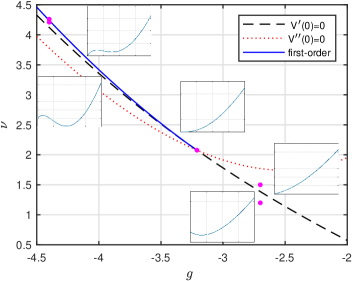
Figure 2: Phase diagram for $p(t)=e^{-t^{3}-gt^{2}-\nu t}$. The five marked points with their effective potentials are those shown in Figure 3.

By Theorem 1.4, there is a transition as the phase boundary $g\mapsto(g,\nu_{c}(g))$ is traversed in the direction of decreasing $g$:

• On the second-order curve, $\chi$ and $\mathbb{E}L$ are of order $N^{1/2}$ and $\rho=0$.

• At the tricritical point, $\chi$ and $\mathbb{E}L$ are of order $N^{2/3}$ and $\rho=0$.

• On the first-order curve, $\chi$ is of order $N^{1/2}$, $\mathbb{E}L$ is of order $N$, and $\rho=\dot{V}(t_{0})>0$.

This is a density transition, from zero to positive density. Note that, by definition, $\dot{V}=\frac{\partial V}{\partial\nu}$ when $p$ is given by (1.29).

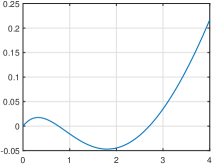
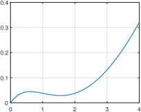
dense phase near first-order curve $(-4.4,4.21)$                     dilute phase near first-order curve $(-4.4,4.26)$

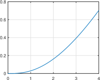
tricritical point

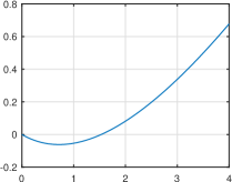
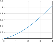
dense phase near second-order curve $(-2.7,1.2)$                     dilute phase near second-order curve $(-2.7,1.5)$

Figure 3: Effective potential $V$ vs $t$ for several values of $(g,\nu)$.

First-order curve. The density $\rho$ is discontinuous when crossing the first-order curve, since its value on the first-order curve is $\dot{V}(t_{0})>0$ whereas its value in the dilute phase is zero. However, the density is continuous at the first-order curve for the one-sided approach from the dense phase. This can be understood from the behaviour of the effective potential: as the first-order curve is approached from the dense phase, $t_{0}$ remains bounded away from zero and $\dot{V}(t_{0})$ does not vanish (upper two images in Figure 3). The density discontinuity on the first-order curve is in contrast to the continous behaviour on the second-order curve. As the second-order curve (or tricritical point) is approached from the dense phase, $t_{0}$ decreases continuously to zero and $\dot{V}(t_{0})\downarrow 0$ (lower two images in Figure 3).

In the limit $N\rightarrow\infty$, the susceptibility has finite limit $\frac{1-V^{\prime}(0)}{V^{\prime}(0)}$ as the first-order curve is approached from the dilute phase, whereas it is divergent on the first-order curve. This is typical of a first-order transition.

Second-order curve and tricritical point. The detailed asymptotic behaviour of the divergence of the susceptibility and the vanishing of the density, at the second-order curve and tricritical point, are as described in the following theorem. The theorem also describes the phase boundary at the tricritical point. Its proof is given in Section 4.

Theorem 1.5 relies on numerical analysis of the effective potential for $p$ given by (1.29), as discussed above. The precise conclusions from this numerical analysis are stated in Section 4.1. We emphasise that the effective potential is a function of a single real variable, and thus we believe that with effort this numerical input could be replaced by rigorous analysis (perhaps with computer assistance), but we do not pursue this.

In the theorem, we consider a line segment

$$(g(s),\nu(s))=(g(0)+sm_{1},\nu(0)+sm_{2})\qquad(s\in[0,1])$$ (1.31)

that approaches a base point $(g(0),\nu(0))$ as $s\downarrow 0$. We write ${\bf m}=(m_{1},m_{2})$ for its direction. The base point may be either the tricritical point or a point on the second-order curve.

Theorem 1.5.

Let $p$ be given by (1.29).

(i) The phase boundary $\nu_{c}(g)$ is differentiable with respect to $g$ at the tricritical point, with slope $-M_{2}$. However, its left and right second derivatives differ at the tricritical point.

(ii) The vector ${\bf n}=(M_{2},M_{1})$ is normal along the second-order curve. Along a line segment (1.31) approaching a point on the second-order curve, or the tricritical point, from the dilute phase with direction satisfying ${\bf m}\cdot{\bf n}\neq 0$ (nontangential at the given point), the infinite-volume susceptibility $\chi=\frac{1-V^{\prime}(0)}{V^{\prime}(0)}$ diverges as

$$\chi=\frac{1-V^{\prime}(0)}{V^{\prime}(0)}\sim\frac{1}{|{\bf m}\cdot{\bf n}|s}.$$ (1.32)

(iii) Along a line sement (1.31) approaching a point on the second-order curve from the dense phase with direction satisfying ${\bf m}\cdot{\bf n}\neq 0$ (nontangential at the given point), the density $\rho$ vanishes as

$$\rho\sim\frac{M_{1}}{1-M_{1}}|{\bf m}\cdot{\bf n}|s\qquad\text{(here $1-M_{1}>0$).}$$ (1.33)

There exists an arc of the second-order curve adjacent to the tricritical point, such that under tangential approach to a point on that arc, $\rho\sim Bs^{2}$ with $B>0$.
There are positive constants $B_{0},B_{1},B_{2},B_{3}$ such that as the tricritical point is approached,

$$\rho\sim\begin{cases}B_{0}{(|{\bf m}\cdot{\bf n}|}s)^{1/2}&\text{(nontangentially from dense phase)}\\ B_{1}s&\text{(tangentially from second-order side)}\\ B_{2}s&\text{(tangentially from first-order side)}\\ B_{3}s&\text{(along first-order curve).}\end{cases}$$ (1.34)

(For the first-order curve, the parametrisation is $(g(s),\nu(s))=(g_{c}-s,\nu_{c}(g-s))$.)

It is possible in general that the susceptibility could have different asymptotic behaviour for the approaches to the second-order curve and the tricritical point, but for the mean-field model there is no difference. However, for the density there is a difference.

2 Integral representation

In this section, we prove integral representations for the two-point function and expected length, in Propositions 2.7–2.8, via the supersymmetric version of the BFS–Dynkin isomorphism theorem [2, Corollary 11.3.7]. These integral representations are in terms of the effective potential and provide the basis for the proofs of Theorems 1.3–1.4. We begin with brief background concerning Grassmann integration. Further background and history for the isomorphism theorem can be found in [2, Chapter 11].

2.1 Grassmann algebra and the integral representation

2.1.1 Grassman algebra

We define a Grassmann algebra $\mathcal{N}_{1}$ with two generators $\psi,\bar{\psi}$ (the bar is only notational and is not a complex conjugate) to consist of linear combinations

$$K=a_{0}+a_{1}\bar{\psi}+a_{2}\psi+a_{3}\bar{\psi}\psi,$$ (2.1)

where each $a_{i}$ is a smooth function $a_{i}:{\mathbb{R}}^{2}\rightarrow{\mathbb{R}}$ written $(u,v)\mapsto a_{i}(u,v)$, and where multiplication of the generators is anti-commutative, i.e.,

$$\bar{\psi}\psi=-\psi\bar{\psi},\qquad\psi\psi=0,\qquad\bar{\psi}\bar{\psi}=0.$$ (2.2)

To make the notation more symmetric, we also combine $(u,v)\in{\mathbb{R}}^{2}$ into a complex variable $\phi$ by

$$\phi=u+iv,\qquad\bar{\phi}=u-iv.$$ (2.3)

We call $(\phi,\bar{\phi})$ a bosonic variable, $(\psi,\bar{\psi})$ a fermionic variable, and $\Phi=(\phi,\bar{\phi},\psi,\bar{\psi})$ a supervariable. Elements of the Grassmann algebra $\mathcal{N}_{1}$ are called forms. A form with $a_{1}=a_{2}=0$ is called even. An important even form is

$$\Phi^{2}=\phi\bar{\phi}+\psi\bar{\psi}.$$ (2.4)

The above discussion concerns a single boson pair and a single fermion pair. We also have need of the Grassmann algebra $\mathcal{N}_{N}$ with $2N$ anticommuting generators $(\psi_{x},\bar{\psi}_{x})_{x\in\Lambda}$, now with coefficients which are smooth functions from ${\mathbb{R}}^{2N}$ to ${\mathbb{R}}$. The even subalgebra consists of elements of $\mathcal{N}_{N}$ which only involve terms containing products of an even number of generators. We refer to $(\phi_{x},\bar{\phi}_{x})_{x\in\Lambda}$ and $(\psi_{x},\bar{\psi}_{x})_{x\in\Lambda}$ as the boson field and the fermion field, respectively. The combination $\Phi=(\phi_{x},\bar{\phi}_{x},\psi_{x},\bar{\psi}_{x})_{x\in\Lambda}$ is called a superfield, and we write

$$\Phi^{2}=(\Phi^{2}_{x})_{x\in\Lambda}=(\phi_{x}\bar{\phi}_{x}+\psi_{x}\bar{\psi}_{x})_{x\in\Lambda}.$$ (2.5)

Two useful even forms in $\mathcal{N}_{N}$ are

$$(\Phi,\Phi) =\sum_{x\in\Lambda}\Phi_{x}^{2}=\sum_{x\in\Lambda}(\phi_{x}\bar{\phi}_{x}+\psi_{x}\bar{\psi}_{x}),$$ (2.6)

$$(\Phi,-\Delta\Phi) =\sum_{x\in\Lambda}\Big{(}\phi_{x}(-\Delta\bar{\phi})_{x}+\psi_{x}(-\Delta\bar{\psi})_{x}\Big{)},$$ (2.7)

where $-\Delta$ is still defined by (1.1) when applied to the generators $\psi$ and $\bar{\psi}$.

For $p\in{\mathbb{N}}$, consider a $C^{\infty}$ function $F:{\mathbb{R}}^{p}\rightarrow{\mathbb{R}}$. Let $K=(K_{j})_{j\leq p}$ be a collection of even forms, and assume that the degree-zero part $K_{j}^{0}$ of each $K_{j}$ (obtained by setting all fermionic variables to zero) is real. We define a form denoted $F(K)$ by Taylor series about the degree-zero part of $K$, i.e.,

$$F(K)=\sum_{\alpha}\frac{1}{\alpha!}F^{(\alpha)}(K^{0})(K-K^{0})^{\alpha}.$$ (2.8)

Here $\alpha=(\alpha_{j})_{j\leq p}$ is a multi-index, with $\alpha!=\prod_{j=1}^{p}\alpha_{j}!$ and $(K-K^{0})^{\alpha}=\prod_{j=1}^{p}(K_{j}-K_{j}^{0})^{\alpha_{j}}$. The order of the product is immaterial since each $K_{j}-K_{j}^{0}$ is even by assumption. Also, the summation terminates after finitely many terms since each $K_{j}-K_{j}^{0}$ is nilpotent.

For example, for $\Phi^{2}\in\mathcal{N}_{1}$ given by (2.4), for smooth $F:{\mathbb{R}}\rightarrow{\mathbb{R}}$, the previous definition with $p=1$ gives

$$F(\Phi^{2})=F(\phi\bar{\phi})+F^{\prime}(\phi\bar{\phi})\psi\bar{\psi}=F(\phi\bar{\phi})-F^{\prime}(\phi\bar{\phi})\bar{\psi}\psi.$$ (2.9)

2.1.2 Grassmann integration and the integral representation

Given a form $K\in\mathcal{N}_{N}$, we write $K_{2N}$ for its coefficient of $\bar{\psi}_{1}\psi_{1}\cdots\bar{\psi}_{N}\psi_{N}$. This $K_{2N}$ is a function of $(u,v)$, i.e., a function on ${\mathbb{R}}^{2N}$. For example, for the form $K=F(\Phi^{2})$ of (2.9), we have $N=1$ and $K_{2}(u,v)=-F^{\prime}(\phi\bar{\phi})=-F^{\prime}(u^{2}+v^{2})$. In general, the superintegral of $K$ is defined by

$$\int_{{\mathbb{R}}^{2N}}D\Phi\,K=\frac{1}{\pi^{N}}\int_{{\mathbb{R}}^{2N}}K_{2N}(u,v)\,du\,dv,$$ (2.10)

assuming that $K_{2N}$ decays sufficiently rapidly that the Lebesgue integral on the right-hand side exists. The notation $D\Phi$ signifies that $K$ is a form for the superfield $\Phi=(\phi_{x},\bar{\phi}_{x},\psi_{x},\bar{\psi}_{x})_{x\in\Lambda}$. This will be useful to distinguish superfields when more than one are in play. The factor $\pi^{-N}$ in the definition simplifies the conclusions of the next example and theorem.

Example 2.1.

If $F:{\mathbb{R}}\rightarrow{\mathbb{R}}$ decays sufficiently rapidly then

$$\int_{{\mathbb{R}}^{2}}D\Phi\,F(\Phi^{2})=F(0).$$ (2.11)

In fact, after conversion to polar coordinates, using $\frac{1}{\pi}\,du\,dv=dr^{2}\,\frac{1}{2\pi}d\theta$, the definition gives

$$\int_{{\mathbb{R}}^{2}}D\Phi\,F(\Phi^{2})=-\int_{{\mathbb{R}}^{2}}F^{\prime}(r^{2})\frac{1}{\pi}\,du\,dv=-\int_{0}^{\infty}F^{\prime}(t)dt=F(0),$$ (2.12)

as claimed.

The supersymmetric version of the BFS–Dynkin isomorphism theorem (see, for example, [2, Corollary 11.3.7]), relates random walks and superfields via an exact equality, as follows.

Theorem 2.2.

Let $F:{\mathbb{R}}^{N}\rightarrow{\mathbb{R}}$ be such that $e^{\epsilon\sum_{z\in\Lambda}t_{z}}F(t)$ is a Schwartz function for some $\epsilon>0$. Then

$$\int_{0}^{\infty}E_{x}\big{(}F(L_{T})\mathbbm{1}_{X(T)=y}\big{)}\,dT=\int_{{\mathbb{R}}^{2N}}D\Phi\,e^{-(\Phi,-\Delta\Phi)}F(\Phi^{2})\,\bar{\phi}_{x}\phi_{y},$$ (2.13)

where $\Delta$ is the generator (defined in (1.1)) of the random walk $X=(X(t))_{t\geq 0}$ with expectation $E_{x}$, and $L_{T}$ is the local time.

By definition, the two-point function (1.3) and expected length (1.6) are given by expressions like the left-hand side of (2.13), which therefore can be rewritten as the right-hand side.

2.1.3 Block-spin renormalisation

The next lemma gives a way to rewrite the exponential factor on the right-hand side of (2.13) as an integral over a single constant block-spin superfield $\mathrm{Z}=(\zeta,\bar{\zeta},\xi,\bar{\xi})$. The application of this lemma can be regarded as a single block-spin renormalisation group step, as in [2, Section 1.4]. For the statement of the lemma, we use the notation

$$(\mathrm{Z}-\Phi,\mathrm{Z}-\Phi)=\sum_{x\in\Lambda}(\mathrm{Z}-\Phi_{x})^{2}=\sum_{x\in\Lambda}\Big{(}(\zeta-\phi_{x})(\bar{\zeta}-\bar{\phi}_{x})+(\xi-\psi_{x})(\bar{\xi}-\bar{\psi}_{x})\Big{)}.$$ (2.14)

Lemma 2.3.

For a superfield $\Phi=(\phi,\bar{\phi},\psi,\bar{\psi})=(\phi_{x},\bar{\phi}_{x},\psi_{x},\bar{\psi}_{x})_{x\in\Lambda}$,

$$e^{-(\Phi,-\Delta\Phi)}=\int_{{\mathbb{R}}^{2}}D\mathrm{Z}\,e^{-(\mathrm{Z}-\Phi,\mathrm{Z}-\Phi)}.$$ (2.15)

Proof.

Let $A\phi=N^{-1}\sum_{x\in\Lambda}\phi_{x}$. Since cross terms vanish,

$$\sum_{x\in\Lambda}(\zeta-\phi_{x})(\bar{\zeta}-\bar{\phi}_{x}) =\sum_{x\in\Lambda}((\zeta-A\phi)+(A\phi-\phi_{x}))((\bar{\zeta}-A\bar{\phi})+(A\bar{\phi}-\bar{\phi}_{x}))$$

$$=N(\zeta-A\phi)(\bar{\zeta}-A\bar{\phi})+\sum_{x\in\Lambda}(A\phi-\phi_{x})(A\bar{\phi}-\bar{\phi}_{x}).$$ (2.16)

By definition of $\Delta$, and since $\sum_{x\in\Lambda}(\Delta f)_{x}=0$, the last term on the right-hand side is

$$\sum_{x\in\Lambda}(A\phi-\phi_{x})(A\bar{\phi}-\bar{\phi}_{x})=\sum_{x\in\Lambda}(A\phi-\phi_{x})(\Delta\bar{\phi})_{x}=-\sum_{x\in\Lambda}\phi_{x}(\Delta\bar{\phi})_{x}.$$ (2.17)

The fermionic part is completely analogous. Therefore, with $A\Phi=(A\phi,A\bar{\phi},A\psi,A\bar{\psi})$,

$$(\mathrm{Z}-\Phi,\mathrm{Z}-\Phi)=N(\mathrm{Z}-A\Phi)^{2}+(\Phi,-\Delta\Phi),$$ (2.18)

and hence

$$\int_{{\mathbb{R}}^{2}}D\mathrm{Z}\,e^{-(\mathrm{Z}-\Phi,\mathrm{Z}-\Phi)}=e^{-(\Phi,-\Delta\Phi)}\int_{{\mathbb{R}}^{2}}D\mathrm{Z}\,e^{-N(\mathrm{Z}-A\Phi)^{2}}.$$ (2.19)

In the integral on the right-hand side, we make the change of variables $\zeta\mapsto\zeta+A\phi$, $\xi\mapsto\xi+A\psi$, and similarly for $\bar{\zeta},\bar{\xi}$. The bosonic change of variables is the usual one for Lebesgue integration, and the fermionic change of variables maintains the same $\bar{\xi}\xi$ term in $e^{-N(\mathrm{Z}-A\Phi)^{2}}$. Thus the integral is unchanged and hence is equal to $\int_{{\mathbb{R}}^{2}}D\mathrm{Z}\,e^{-N\mathrm{Z}^{2}}$, which is $1$ by (2.11). This completes the proof.  

2.2 Effective potential

Definition 2.4.

Given a (smooth) function $p:[0,\infty)\rightarrow[0,\infty)$ such that the following integral exists, the effective potential $V:[0,\infty)\rightarrow{\mathbb{R}}$ is defined by

$$e^{-V(\mathrm{Z}^{2})}=\int_{{\mathbb{R}}^{2}}D\Phi\,e^{-(\mathrm{Z}-\Phi)^{2}}p(\Phi^{2}).$$ (2.20)

That the right-hand side truly is a function of the form $\mathrm{Z}^{2}$ is proved in Lemma 2.10, which we defer to Section 2.4. The consistency of this definition of $V$ with the formula given in (1.14) is established in Proposition 2.5.

The proof of the next proposition appeals to Lemma 2.10. Recall that $I_{1}$ is a modified Bessel function of the first kind.

Proposition 2.5.

Fix $\mathrm{Z}=(\zeta,\bar{\zeta},\xi,\bar{\xi})$. For any bounded smooth function $p:[0,\infty)\rightarrow[0,\infty)$ such that the integrals exist,

$$\int_{{\mathbb{R}}^{2}}D\Phi\,e^{-(\mathrm{Z}-\Phi)^{2}}p(\Phi^{2})=e^{-\mathrm{Z}^{2}}\left(p(0)+\int_{0}^{\infty}p(s)e^{-s}\sqrt{\frac{\mathrm{Z}^{2}}{s}}I_{1}(2\sqrt{\mathrm{Z}^{2}s})ds\right),$$ (2.21)

and hence

$$V(t)=t-\log(p(0)+v(t)),\qquad v(t)=\int_{0}^{\infty}p(s)e^{-s}\sqrt{\frac{t}{s}}I_{1}(2\sqrt{ts})ds.$$ (2.22)

Proof.

We denote the left-hand side of (2.21) by $F=F(\zeta,\bar{\zeta},\xi,\bar{\xi})$. By Lemma 2.10, $F$ is a function of $\mathrm{Z}^{2}$ so it suffices to prove that

$$F(\zeta,\bar{\zeta},0,0)=e^{-|\zeta|^{2}}\left(p(0)+\int_{0}^{\infty}p(s)e^{-s}|\zeta|\frac{1}{\sqrt{s}}I_{1}(2|\zeta|\sqrt{s})ds\right).$$ (2.23)

Let $\tilde{p}(s)=p(s)e^{-s}$. With $\xi=\bar{\xi}=0$, the integrand of the left-hand side of (2.21) becomes

$$e^{-|\zeta|^{2}}e^{\zeta\bar{\phi}+\bar{\zeta}\phi}\tilde{p}(\Phi^{2}) =e^{-|\zeta|^{2}}e^{\zeta\bar{\phi}+\zeta\phi}\left(\tilde{p}(|\phi|^{2})+\tilde{p}^{\prime}(|\phi|^{2})\psi\bar{\psi}\right).$$ (2.24)

Therefore, by the definition (2.10) of the integral, and with $I_{0}(z)=\frac{1}{2\pi}\int_{0}^{2\pi}e^{z\cos\theta}d\theta$ the modified Bessel function of the first kind,

$$F(\zeta,\bar{\zeta},0,0) =-e^{-|\zeta|^{2}}\int_{{\mathbb{R}}^{2}}e^{\zeta re^{-i\theta}+\bar{\zeta}re^{i\theta}}\tilde{p}^{\prime}(r^{2})\frac{dr^{2}\,d\theta}{2\pi}$$

$$=-e^{-|\zeta|^{2}}\int_{0}^{\infty}ds\,\tilde{p}^{\prime}(s)\int_{0}^{2\pi}e^{\zeta\sqrt{s}e^{-i\theta}+\bar{\zeta}\sqrt{s}e^{i\theta}}\frac{d\theta}{2\pi}$$

$$=-e^{-|\zeta|^{2}}\int_{0}^{\infty}ds\,\tilde{p}^{\prime}(s)\int_{0}^{2\pi}e^{2|\zeta|\sqrt{s}\cos\theta}\frac{d\theta}{2\pi}$$

$$=-e^{-|\zeta|^{2}}\int_{0}^{\infty}\tilde{p}^{\prime}(s)I_{0}(2|\zeta|\sqrt{s})\,ds$$

$$=e^{-|\zeta|^{2}}\left(\tilde{p}(0)+\int_{0}^{\infty}\tilde{p}(s)I_{0}^{\prime}(2|\zeta|\sqrt{s})|\zeta|\frac{1}{\sqrt{s}}ds\right),$$ (2.25)

where we used integration by parts for the last equality, together with our assumption that $p$ is bounded at infinity (this can certainly be weakened). Since $I_{0}^{\prime}=I_{1}$, the proof is complete.  

Next, for later use, we state and prove a lemma that shows how the effective potential arises in various integrals. As usual, we write $V^{\prime}=\frac{dV}{dt}$ and $\dot{V}=\frac{\partial V}{\partial\epsilon}|_{\epsilon=0}$ (with the $\epsilon$-dependence as in (1.7), see (1.26)). We also write $Q^{\prime}=1-V^{\prime}$. We define forms $k_{*}=k_{*}(\mathrm{Z}^{2},\zeta,\bar{\zeta})$ by:

$$\begin{gathered}k_{0}=\zeta Q^{\prime}(\mathrm{Z}^{2}),\qquad\bar{k}_{0}=\bar{\zeta}Q^{\prime}(\mathrm{Z}^{2}),\qquad k_{00}=Q^{\prime}(\mathrm{Z}^{2})+Q^{\prime}(\mathrm{Z}^{2})^{2}|\zeta|^{2}-V^{\prime\prime}(\mathrm{Z}^{2})|\zeta|^{2},\\ k_{+}=\dot{V}(\mathrm{Z}^{2}),\qquad k_{0+}=\zeta(Q^{\prime}(\mathrm{Z}^{2})\dot{V}(\mathrm{Z}^{2})+\dot{V}^{\prime}(\mathrm{Z}^{2})),\qquad\bar{k}_{0+}=\bar{\zeta}(Q^{\prime}(\mathrm{Z}^{2})\dot{V}(\mathrm{Z}^{2})+\dot{V}^{\prime}(\mathrm{Z}^{2})),\\ k_{00+}=k_{00}\dot{V}(\mathrm{Z}^{2})+\big{(}1+2Q^{\prime}(\mathrm{Z}^{2})|\zeta|^{2}\big{)}\dot{V}^{\prime}(\mathrm{Z}^{2})+\dot{V}^{\prime\prime}(\mathrm{Z}^{2})|\zeta|^{2}.\end{gathered}$$ (2.26)

Lemma 2.6.

The following integral formulas hold:

$$\begin{gathered}\int_{{\mathbb{R}}^{2}}D\Phi\,\phi p(\Phi^{2})e^{-(\mathrm{Z}-\Phi)^{2}}=k_{0}e^{-V(\mathrm{Z}^{2})},\qquad\int_{{\mathbb{R}}^{2}}D\Phi\,\bar{\phi}p(\Phi^{2})e^{-(\mathrm{Z}-\Phi)^{2}}=\bar{k}_{0}e^{-V(\mathrm{Z}^{2})},\\ \int_{{\mathbb{R}}^{2}}D\Phi\,\bar{\phi}\phi p(\Phi^{2})e^{-(\mathrm{Z}-\Phi)^{2}}=k_{00}e^{-V(\mathrm{Z}^{2})},\qquad\int_{{\mathbb{R}}^{2}}D\Phi\,\Phi^{2}p(\Phi^{2})e^{-(\mathrm{Z}-\Phi)^{2}}=k_{+}e^{-V(\mathrm{Z}^{2})},\\ \int_{{\mathbb{R}}^{2}}D\Phi\,\phi\Phi^{2}p(\Phi^{2})e^{-(\mathrm{Z}-\Phi)^{2}}=k_{0+}e^{-V(\mathrm{Z}^{2})},\qquad\int_{{\mathbb{R}}^{2}}D\Phi\,\bar{\phi}\Phi^{2}p(\Phi^{2})e^{-(\mathrm{Z}-\Phi)^{2}}=\bar{k}_{0+}e^{-V(\mathrm{Z}^{2})},\\ \int_{{\mathbb{R}}^{2}}D\Phi\,\bar{\phi}\phi\Phi^{2}p(\Phi^{2})e^{-(\mathrm{Z}-\Phi)^{2}}=k_{00+}e^{-V(\mathrm{Z}^{2})}.\end{gathered}$$ (2.27)

Proof.

Given $h:\Lambda\rightarrow\mathbb{C}$, let $(\mathrm{Z}+h)^{2}=(\zeta+h)(\bar{\zeta}+\bar{h})+\xi\bar{\xi}$. There is no fermionic partner for $h$ in $(\mathrm{Z}+h)^{2}$. Completion of the square and the definition of $V$ give

$$\int_{{\mathbb{R}}^{2}}D\Phi\,e^{-(\mathrm{Z}-\Phi)^{2}}p(\Phi^{2})e^{h\bar{\phi}+\bar{h}\phi}=e^{h\bar{h}}e^{h\bar{\zeta}+\bar{h}\zeta}\int_{{\mathbb{R}}^{2}}D\Phi\,e^{-(\mathrm{Z}-\Phi+h)^{2}}p(\Phi^{2})=e^{h\bar{h}}e^{h\bar{\zeta}+\bar{h}\zeta}e^{-V((\mathrm{Z}+h)^{2})}.$$ (2.28)

Therefore, using $\frac{\partial\bar{h}}{\partial h}=0$, we obtain

$$\int_{{\mathbb{R}}^{2}}D\Phi\,\bar{\phi}p(\Phi^{2})e^{-(\mathrm{Z}-\Phi)^{2}} =\frac{\partial}{\partial h}\Big{|}_{h=0}\int_{{\mathbb{R}}^{2}}D\Phi\,e^{-(\mathrm{Z}-\Phi)^{2}}p(\Phi^{2})e^{h\bar{\phi}+\bar{h}\phi}$$

$$=\frac{\partial}{\partial h}\Big{|}_{h=0}e^{h\bar{h}}e^{h\bar{\zeta}+\bar{h}\zeta}e^{-V((\mathrm{Z}+h)^{2})}=\bar{\zeta}(1-V^{\prime}(\mathrm{Z}^{2}))e^{-V(\mathrm{Z}^{2})}.$$ (2.29)

The first and third equalities in (2.27) follow similarly. For the fourth, with $V^{(\epsilon)}$ the effective potential for $p(s)e^{-\epsilon s}$, we use

$$\int_{{\mathbb{R}}^{2}}D\Phi\,\Phi^{2}p(\Phi^{2})e^{-(\mathrm{Z}-\Phi)^{2}} =-\frac{\partial}{\partial\epsilon}\Big{|}_{\epsilon=0}\int_{{\mathbb{R}}^{2}}D\Phi\,p(\Phi^{2})e^{-\epsilon\Phi^{2}}e^{-(\mathrm{Z}-\Phi)^{2}}$$

$$=-\frac{\partial}{\partial\epsilon}\Big{|}_{\epsilon=0}e^{-V^{(\epsilon)}(\mathrm{Z}^{2})}=\dot{V}(\mathrm{Z}^{2})e^{-V(\mathrm{Z}^{2})}.$$ (2.30)

The remaining three identities follow, e.g., from

$$\int_{{\mathbb{R}}^{2}}D\Phi\,\bar{\phi}\Phi^{2}p(\Phi^{2})e^{-(\mathrm{Z}-\Phi)^{2}} =-\frac{\partial}{\partial\epsilon}\Big{|}_{\epsilon=0}\int_{{\mathbb{R}}^{2}}D\Phi\,\bar{\phi}p(\Phi^{2})e^{-\epsilon\Phi^{2}}e^{-(\mathrm{Z}-\Phi)^{2}},$$ (2.31)

together with differentiation of the right-hand sides of the first three identities with respect to $\epsilon$.  

2.3 Two-point function and expected length

We now have what is needed to prove integral representations for the two-point function and expected length, in the next two propositions.

Proposition 2.7.

The two-point function is given by

$$G_{01} =\int_{{\mathbb{R}}^{2}}D\mathrm{Z}\,e^{-NV(\mathrm{Z}^{2})}(1-V^{\prime}(\mathrm{Z}^{2}))^{2}|\zeta|^{2},$$ (2.32)

$$G_{00} =\ (1-V^{\prime}(0))+G_{01}-\int_{{\mathbb{R}}^{2}}D\mathrm{Z}\,e^{-NV(\mathrm{Z}^{2})}V^{\prime\prime}(\mathrm{Z}^{2})|\zeta|^{2}.$$ (2.33)

Proof.

By the the definition of the two-point function in (1.3), followed by the supersymmetric BFS–Dynkin isomorphism (2.13) and the block-spin transformation of Lemma 2.3,

$$G_{xy} =\int_{0}^{\infty}E_{x}(p_{N}(L_{T})\mathbbm{1}_{X(T)=y})\,dT$$

$$=\int_{{\mathbb{R}}^{2N}}D\Phi\,e^{-(\Phi,-\Delta\Phi)}\bar{\phi}_{x}\phi_{y}p_{N}(\Phi^{2})$$

$$=\int_{{\mathbb{R}}^{2}}D\mathrm{Z}\,\int_{{\mathbb{R}}^{2N}}D\Phi\,\bar{\phi}_{x}\phi_{y}p_{N}(\Phi^{2})e^{-(\mathrm{Z}-\Phi)^{2}}.$$ (2.34)

The integral over ${\mathbb{R}}^{2N}$ on the right-hand side of (2.34) factorises into a product of $N$ integrals over ${\mathbb{R}}^{2}$ (each an integral with respect to $\Phi_{x}$ at a single point $x$). With the definition of the effective potential in Definition 2.4, and with the first line of (2.27), this leads to

$$G_{01} =\int_{{\mathbb{R}}^{2}}D\mathrm{Z}\,e^{-(N-2)V(\mathrm{Z}^{2})}\left(\int_{{\mathbb{R}}^{2}}D\Phi_{0}\,\bar{\phi}_{0}p(\Phi_{0}^{2})e^{-(\mathrm{Z}-\Phi_{0})^{2}}\right)\left(\int_{{\mathbb{R}}^{2}}D\Phi_{1}\,\phi_{1}p(\Phi_{1}^{2})e^{-(\mathrm{Z}-\Phi_{1})^{2}}\right)$$

$$=\int_{{\mathbb{R}}^{2}}D\mathrm{Z}\,e^{-NV(\mathrm{Z}^{2})}(1-V^{\prime}(\mathrm{Z}^{2}))^{2}|\zeta|^{2}.$$ (2.35)

Similarly, by the third equality of (2.27),

$$G_{00} =\int_{{\mathbb{R}}^{2}}D\mathrm{Z}\,e^{-(N-1)V(\mathrm{Z}^{2})}\int_{{\mathbb{R}}^{2}}D\Phi_{0}\,\bar{\phi}_{0}\phi_{0}p(\Phi_{0}^{2})e^{-(\mathrm{Z}-\Phi_{0})^{2}}$$

$$=\int_{{\mathbb{R}}^{2}}D\mathrm{Z}\,e^{-NV(\mathrm{Z}^{2})}\big{(}(1-V^{\prime}(\mathrm{Z}^{2}))+(1-V^{\prime}(\mathrm{Z}^{2}))^{2}|\zeta|^{2}-V^{\prime\prime}(\mathrm{Z}^{2})|\zeta|^{2}\big{)}$$

$$=(1-V^{\prime}(0))+G_{01}-\int_{{\mathbb{R}}^{2}}D\mathrm{Z}\,e^{-NV(\mathrm{Z}^{2})}V^{\prime\prime}(\mathrm{Z}^{2})|\zeta|^{2},$$ (2.36)

where in the last line we used (2.11) for the first term and (2.35) for the second. This completes the proof.  

For the expected length the general procedure is the same. With $k_{*}$ defined by (2.26), let

$$K_{0xy} =\begin{cases}\bar{k}_{0}k_{0}k_{+}&(x=1,\,y=2)\\ k_{00}k_{+}&(x=0,\,y=1)\\ \bar{k}_{0}k_{0+}&(x=y=1)\\ k_{00+}&(x=y=0).\end{cases}$$ (2.37)

Proposition 2.8.

The expected length is given by

$$\mathbb{E}L =\frac{1}{\chi}\Big{(}(N-1)(N-2)\int_{{\mathbb{R}}^{2}}D\mathrm{Z}\,e^{-NV(\mathrm{Z}^{2})}K_{012}$$

$$\quad\quad+(N-1)\int_{{\mathbb{R}}^{2}}D\mathrm{Z}\,e^{-NV(\mathrm{Z}^{2})}(K_{001}+2K_{011})+\int_{{\mathbb{R}}^{2}}D\mathrm{Z}\,e^{-NV(\mathrm{Z}^{2})}K_{000}\Big{)}.$$ (2.38)

Proof.

By (1.6) and $T=\sum_{x\in\Lambda}L_{T,x}$,

$$\mathbb{E}L =\frac{1}{\chi}\sum_{x,y\in\Lambda}\int_{0}^{\infty}E_{0}(L_{T,y}p_{N}(L_{T})\mathbbm{1}_{X(T)=x})dT.$$ (2.39)

By the supersymmetric BFS–Dynkin isomorphism (2.13) followed by the block-spin transformation of Lemma 2.3,

$$\mathbb{E}L =\frac{1}{\chi}\sum_{x,y\in\Lambda}\int_{{\mathbb{R}}^{2N}}D\Phi\,\bar{\phi}_{0}\phi_{x}\Phi^{2}_{y}p_{N}(\Phi^{2})e^{-(\Phi,-\Delta\Phi)}$$

$$=\frac{1}{\chi}\sum_{x,y\in\Lambda}\int_{{\mathbb{R}}^{2}}D\mathrm{Z}\,\int_{{\mathbb{R}}^{2N}}D\Phi\,\bar{\phi}_{0}\phi_{x}\Phi^{2}_{y}p_{N}(\Phi^{2})e^{-(\mathrm{Z}-\Phi)^{2}}.$$ (2.40)

By symmetry, it suffices to show that

$$\int_{{\mathbb{R}}^{2N}}D\Phi\,\bar{\phi}_{0}\phi_{x}\Phi^{2}_{y}p(\Phi^{2})e^{-(\mathrm{Z}-\Phi)^{2}}=e^{-NV(\mathrm{Z}^{2})}K_{0xy}.$$ (2.41)

For the case of $0,x,y$ distinct, since the $N-3$ integrals for the factors with $z\neq 0,x,y$ are the same,

$$\int_{{\mathbb{R}}^{2N}}D\Phi\,\bar{\phi}_{0}\phi_{x}\Phi^{2}_{y}p(\Phi^{2})e^{-(\mathrm{Z}-\Phi)^{2}}=e^{-(N-3)V(\mathrm{Z}^{2})}\left(\int_{{\mathbb{R}}^{2}}D\Phi_{0}\,\bar{\phi}_{0}p(\Phi_{0}^{2})e^{-(\mathrm{Z}-\Phi_{0})^{2}}\right)\\ \times\left(\int_{{\mathbb{R}}^{2}}D\Phi_{x}\,\phi_{x}p(\Phi_{x}^{2})e^{-(\mathrm{Z}-\Phi_{x})^{2}}\right)\left(\int_{{\mathbb{R}}^{2}}D\Phi_{y}\,\Phi^{2}_{y}p(\Phi_{y}^{2})e^{-(\mathrm{Z}-\Phi_{y})^{2}}\right),$$ (2.42)

and (2.41) follows from the definitions of $k_{0},\bar{k}_{0},k_{+}$. The other cases are similar.  

2.4 Supersymmetry

In this section, we prove Lemma 2.10, which was used in the proof of Proposition 2.5. It is possible to give a more direct proof of Proposition 2.5 without using the notion of supersymmetry. However, the proof using Lemma 2.10 is particularly elegant.

The supersymmetry generator is the anti-derivation defined by

$$Q=\psi\frac{\partial}{\partial\phi}+\bar{\psi}\frac{\partial}{\partial\bar{\phi}}-\phi\frac{\partial}{\partial\psi}+\bar{\phi}\frac{\partial}{\partial\bar{\psi}}.$$ (2.43)

We say that $F=F(\phi,\bar{\phi},\psi,\bar{\psi})$ is supersymmetric if $QF=0$. The next lemma is [6, Lemma A.4].

Lemma 2.9.

If $F$ is even and supersymmetric then $F=f(\Phi^{2})$ for some function $f$.

Proof.

We write $F=G+H\psi\bar{\psi}$, and use subscripts to denote partial derivatives. It suffices to show that there is a function $f$ such that $G(\phi,\bar{\phi})=f(|\phi|^{2})$ and $H(\phi,\bar{\phi})=f^{\prime}(|\phi|^{2})$. Since

$$0=QF =G_{\phi}\psi+G_{\bar{\phi}}\bar{\psi}-\phi H\bar{\psi}-\bar{\phi}H\psi,$$ (2.44)

we see that $G_{\phi}=\bar{\phi}H$ and $G_{\bar{\phi}}=\phi H$. Therefore,

$$\frac{d}{d\theta}G(\phi e^{i\theta},\bar{\phi}e^{-i\theta}) =G_{\phi}(\phi e^{i\theta},\bar{\phi}e^{-i\theta})\phi ie^{i\theta}+G_{\bar{\phi}}(\phi e^{i\theta},\bar{\phi}e^{-i\theta})\bar{\phi}(-i)e^{-i\theta}$$

$$=\bar{\phi}e^{-i\theta}H(\phi e^{i\theta},\bar{\phi}e^{-i\theta})\phi ie^{i\theta}+\phi e^{i\theta}H(\phi e^{i\theta},\bar{\phi}e^{-i\theta})\bar{\phi}(-i)e^{-i\theta}=0.$$ (2.45)

This implies that there is a function $f$ as required.  

Lemma 2.10.

The integral $\int_{{\mathbb{R}}^{2}}D\Phi\,e^{-(\mathrm{Z}-\Phi)^{2}}p(\Phi^{2})$ is an even supersymmetric form, and hence is a function of $\mathrm{Z}^{2}$.

Proof.

Let $F=F(\zeta,\bar{\zeta},\xi,\bar{\xi})=\int_{{\mathbb{R}}^{2}}D\Phi\,e^{-(\mathrm{Z}-\Phi)^{2}}p(\Phi^{2})$. Since $p(\Phi^{2})$ is even, only even contributions in $\psi,\bar{\psi}$ from

$$e^{-(\mathrm{Z}-\Phi)^{2}}=e^{-|\zeta-\phi|^{2}}(1-(\xi-\psi)(\bar{\xi}-\bar{\psi}))$$ (2.46)

can contribute to the integral. Thus, within the integral, the above right-hand side can be replaced by $e^{-|\zeta-\phi|^{2}}(1-\xi\bar{\xi}-\psi\bar{\psi})$, and we see that $F$ is even in $\xi,\bar{\xi}$.

To see that $F$ is supersymmetric, let $Q_{\mathrm{Z}}$ act on $\mathrm{Z}=(\zeta,\bar{\zeta},\xi,\bar{\xi})$ and $Q_{\Phi}$ on $\Phi=(\phi,\bar{\phi},\psi,\bar{\psi})$. By definition,

$$e^{-(\mathrm{Z}-\Phi)^{2}}=e^{-\Phi^{2}}e^{-\mathrm{Z}^{2}}e^{K}\quad\text{with}\quad K=\zeta\bar{\phi}+\phi\bar{\zeta}+\xi\bar{\psi}+\psi\bar{\xi}.$$ (2.47)

Let $\tilde{p}(\Phi^{2})=p(\Phi^{2})e^{-\Phi^{2}}$. Since $Q_{\mathrm{Z}}$ is an anti-derivation, since $Q_{\mathrm{Z}}e^{-\mathrm{Z}^{2}}=0$ and $Q_{\Phi}\tilde{p}(\Phi^{2})=0$ (by [2, Example 11.4.4]), and since $Q_{\mathrm{Z}}e^{K}=-Q_{\Phi}e^{K}$,

$$Q_{\mathrm{Z}}F =e^{-\mathrm{Z}^{2}}Q_{\mathrm{Z}}\Big{(}\int_{{\mathbb{R}}^{2}}D\Phi\,e^{K}\tilde{p}(\Phi^{2})\Big{)}=e^{-\mathrm{Z}^{2}}\int_{{\mathbb{R}}^{2}}D\Phi\,(Q_{\mathrm{Z}}e^{K})\tilde{p}(\Phi^{2})$$

$$=e^{-\mathrm{Z}^{2}}\int_{{\mathbb{R}}^{2}}D\Phi\,(-Q_{\Phi}e^{K})\tilde{p}(\Phi^{2})=-e^{-\mathrm{Z}^{2}}\int_{{\mathbb{R}}^{2}}D\Phi\,Q_{\Phi}\Big{(}e^{K}\tilde{p}(\Phi^{2})\Big{)}.$$ (2.48)

The last integrand is in the image of $Q_{\Phi}$, so the integral is zero (see [2, Section 11.4.1]), and hence $F$ is supersymmetric. By Lemma 2.9, $F$ is therefore a function of $\mathrm{Z}^{2}$.  

3 Proof of general results: Theorems 1.3–1.4

The proofs of Theorems 1.3–1.4 amount to application of the Laplace method to the integrals of Propositions 2.7–2.8. The application of the Laplace method depends on whether: (i) the global minimum of the effective potential is attained at zero and only at zero, or (ii) it is attained at a point $t_{0}>0$ with $V(t_{0})<0$ or $V(t_{0})=0$. Case (i) concerns the dilute phase, the second-order curve, and the tricritical point, while case (ii) concerns the dense phase and first-order curve.

3.1 Laplace method

3.1.1 Laplace method: minimum at endpoint

For the dilute phase, the second-order curve, and the tricritical point, we use the following theorem, which can be found, e.g., in [19, p.81]. The theorem can be extended to an asymptotic expansion to all orders, [19, p.86] or [18, p.233], but we do not need the extension. In a corollary to the theorem, we adapt its statement to integrals of the form appearing in Propositions 2.7–2.8.

Theorem 3.1.

Suppose that $V,q:[a,b)\rightarrow{\mathbb{R}}$ ($b=\infty$ is allowed) are such that:
(i) $V$ has a unique global minimum $V(a)$ (as defined at the beginning of Section 1.3),
(ii) $V^{\prime}$ and $q$ are continuous in a neighbourhood of $a$, except possibly at $a$,
(iii) as $t\rightarrow a^{+}$, $V(t)\sim v_{0}(t-a)^{\mu}$, $V^{\prime}(t)\sim\mu v_{0}(t-a)^{\mu-1}$, $q(t)\sim q_{0}(t-a)^{\lambda-1}$, with $v_{0},\mu,\lambda>0$ and $q_{0}\neq 0$,
(iv) $e^{-NV(t)}q(t)$ is integrable for large $N$.
Then

$$\int_{a}^{b}e^{-NV(t)}q(t)dt\sim e^{-NV(a)}\frac{q_{0}}{\mu(v_{0}N)^{\lambda/\mu}}\Gamma\Big{(}\frac{\lambda}{\mu}\Big{)}.$$ (3.1)

Corollary 3.2.

Suppose that the hypotheses on $V$ of Theorem 3.1 hold with $a=0$ and $b=\infty$. Suppose that $F:[0,\infty)^{2}\rightarrow{\mathbb{R}}$ is such that $q(t)=V^{\prime}(t)F(t,t)$ and $q(t)=\partial_{1}F(t,t)$ obey hypotheses (ii) and (iv) of Theorem 3.1, and that, as $t\downarrow 0$,

$$F(t,t) \sim q_{0}t^{\lambda_{0}},\qquad\partial_{1}F(t,t)\sim\lambda_{1}r_{0}t^{\lambda_{1}-1}.$$ (3.2)

If $\lambda_{1}>\lambda_{0}\geq 0$ then

$$\int_{{\mathbb{R}}^{2}}D\mathrm{Z}\,e^{-NV(\mathrm{Z}^{2})}F(\mathrm{Z}^{2},|\zeta|^{2}) \sim e^{-NV(0)}\frac{q_{0}}{(v_{0}N)^{\lambda_{0}/\mu}}\Gamma\left(\frac{\mu+\lambda_{0}}{\mu}\right).$$ (3.3)

If $\lambda_{1}=\lambda_{0}>0$ then

$$\int_{{\mathbb{R}}^{2}}D\mathrm{Z}\,e^{-NV(\mathrm{Z}^{2})}F(\mathrm{Z}^{2},|\zeta|^{2}) \sim e^{-NV(0)}\frac{q_{0}-r_{0}}{(v_{0}N)^{\lambda_{0}/\mu}}\Gamma\left(\frac{\mu+\lambda_{0}}{\mu}\right),$$ (3.4)

where the right-hand side is interpreted as $e^{-NV(0)}o(N^{-\lambda_{0}/\mu})$ if $q_{0}=r_{0}$.
For any $\lambda_{1}>0$ and $\lambda_{0}\geq 0$, the integral is at most $e^{-NV(0)}O(N^{-\lambda_{0}/\mu}+N^{-\lambda_{1}/\mu})$.

Proof.

By definition of the integral, and since $\bar{\xi}\xi=\frac{1}{\pi}dxdy=\frac{1}{2\pi}dr^{2}d\theta$ (as in (2.11)),

$$\int_{{\mathbb{R}}^{2}}D\mathrm{Z}\,e^{-NV(\mathrm{Z}^{2})}F(\mathrm{Z}^{2},|\zeta|^{2})$$

$$\quad=\int_{{\mathbb{R}}^{2}}D\mathrm{Z}\,e^{-NV(|\zeta|^{2})}\Big{(}1-NV^{\prime}(|\zeta|^{2})\xi\bar{\xi}\Big{)}\Big{(}F(|\zeta|^{2},|\zeta|^{2})+\partial_{1}F(|\zeta|^{2},|\zeta|^{2})\xi\bar{\xi}\Big{)}$$

$$\quad=\int_{{\mathbb{R}}^{2}}D\mathrm{Z}\,e^{-NV(|\zeta|^{2})}\Big{(}NV^{\prime}(|\zeta|^{2})F(|\zeta|^{2},|\zeta|^{2})-\partial_{1}F(|\zeta|^{2},|\zeta|^{2})\Big{)}\bar{\xi}\xi$$

$$\quad=\int_{0}^{\infty}e^{-NV(t)}(NV^{\prime}(t)F(t,t)-\partial_{1}F(t,t))\,dt.$$ (3.5)

Now we apply Theorem 3.1. Since $V^{\prime}(t)F(t,t)\sim\mu v_{0}t^{\mu-1}q_{0}t^{\lambda_{0}}$, the power of $N$ arising for this term is $NN^{-(\mu+\lambda_{0})/\mu}=N^{-\lambda_{0}/\mu}$. If $\lambda_{1}>\lambda_{0}\geq 0$ then this dominates the power $N^{-\lambda_{1}/\mu}$ from the $\partial_{1}F(t,t)$ term and yields (3.3). If $\lambda_{1}=\lambda_{0}>0$ then both terms contribute the same power of $N$, and (3.4) follows from $\Gamma((\mu+\lambda_{1})/\mu)=(\lambda_{1}/\mu)\Gamma(\lambda_{1}/\mu)$. Finally, the general upper bound follows immediately from the above considerations.  

3.1.2 Laplace method: minimum at interior point

The following theorem from [19, p.127] more than covers our needs for the case where $V$ attains its unique global minimum in an open interval. Its analyticity assumption could be weakened, but the analyticity does hold in our setting.

Theorem 3.3.

Let $a\in[-\infty,\infty)$ and $b\in(-\infty,\infty]$. Suppose that $V,q:(a,b)\rightarrow{\mathbb{R}}$ are analytic, and that $V$ has a unique global minimum at $t_{0}\in(a,b)$ (as defined at the beginning of Section 1.3) with $V^{\prime}(t_{0})=0$ and $V^{\prime\prime}(t_{0})>0$. Then, assuming that the integral is finite for some $N$,

$$\int_{a}^{b}e^{-NV(t)}q(t)dt\sim 2e^{-NV(t_{0})}\sum_{s=0}^{\infty}\Gamma(s+1/2)\frac{b_{s}}{N^{s+1/2}},$$ (3.6)

with (all functions evaluated at $t_{0}$)

$$b_{0} =\frac{q}{(2V^{\prime\prime})^{1/2}},$$ (3.7)

$$b_{1} =\left(2q^{\prime\prime}-\frac{2V^{\prime\prime\prime}q^{\prime}}{V^{\prime\prime}}+\left[\frac{5V^{\prime\prime\prime 2}}{6V^{\prime\prime 2}}-\frac{V^{\prime\prime\prime\prime}}{2V^{\prime\prime}}\right]q\right)\frac{1}{(2V^{\prime\prime})^{3/2}},$$ (3.8)

and with $b_{s}$ as given in [19] for $s\geq 2$.

Corollary 3.4.

Suppose that $V:(0,\infty)\rightarrow{\mathbb{R}}$ is analytic and has a unique global minimum at $t_{0}\in(0,\infty)$ (as defined at the beginning of Section 1.3) with $V^{\prime}(t_{0})=0$ and $V^{\prime\prime}(t_{0})>0$. Given $F:(0,\infty)^{2}\rightarrow{\mathbb{R}}$, suppose that the functions $C(t)=V^{\prime}(t)F(t,t)$ and $D(t)=\partial_{1}F(t,t)$ are analytic on $(a,b)$ and that $\int_{0}^{\infty}e^{-NV(t)}q(t)\,dt$ is finite for $q=C$ and $q=D$. Then

$$\int_{{\mathbb{R}}^{2}}D\mathrm{Z}\,e^{-NV(\mathrm{Z}^{2})}F(\mathrm{Z}^{2},|\zeta|^{2}) \sim 2e^{-NV(t_{0})}\sum_{s=0}^{\infty}\frac{1}{N^{s+1/2}}\Big{(}c_{s+1}\Gamma(s+3/2)-d_{s}\Gamma(s+1/2)\Big{)},$$ (3.9)

where the coefficients $c_{s}$ and $d_{s}$ are the coefficients $b_{s}$ computed when the function $q$ in Theorem 3.3 is replaced by $C$ and $D$, respectively. Assuming that $\partial_{2}F(t_{0},t_{0})\neq 0$, we have in particular

$$\int_{{\mathbb{R}}^{2}}D\mathrm{Z}\,e^{-NV(\mathrm{Z}^{2})}F(\mathrm{Z}^{2},|\zeta|^{2}) \sim e^{-NV(t_{0})}\frac{1}{N^{1/2}}\frac{\sqrt{2\pi}}{V^{\prime\prime}(t_{0})^{1/2}}\partial_{2}F(t_{0},t_{0}).$$ (3.10)

Proof.

The full expansion follows from Theorem 3.3 and (3.5). Let $A=\frac{\sqrt{2}}{V^{\prime\prime}(t_{0})^{1/2}}\partial_{2}F(t_{0},t_{0})$. For (3.10), since $\Gamma(1/2)=\sqrt{\pi}$, it suffices to show that $c_{1}-2d_{0}=A$. Let $F^{\prime}=\frac{d}{dt}F(t,t)=\partial_{1}F(t,t)+\partial_{2}F(t,t)$. Then

$$C^{\prime} =V^{\prime\prime}F+V^{\prime}F^{\prime},\qquad C^{\prime\prime}=V^{\prime\prime\prime}F+2V^{\prime\prime}F^{\prime}+V^{\prime}F^{\prime\prime}.$$ (3.11)

Since $V^{\prime}(t_{0})=0$ we find from (3.7)–(3.8) that

$$c_{1}-2d_{0} =\frac{1}{(2V^{\prime\prime})^{3/2}}\left(2C^{\prime\prime}-\frac{2V^{\prime\prime\prime}C^{\prime}}{V^{\prime\prime}}\right)-2\frac{\partial_{1}F}{(2V^{\prime\prime})^{1/2}}$$

$$=\frac{1}{(2V^{\prime\prime})^{3/2}}\left(2(V^{\prime\prime\prime}F+2V^{\prime\prime}F^{\prime})-\frac{2V^{\prime\prime\prime}V^{\prime\prime}F}{V^{\prime\prime}}\right)-2\frac{\partial_{1}F}{(2V^{\prime\prime})^{1/2}},$$ (3.12)

and after simplification the right-hand side is equal to $A$.  

On the first-order curve, $V$ has global minima $V(0)=V(t_{0})$ with $V^{\prime}(0)>0$ and $V^{\prime\prime}(t_{0})>0$ (by smoothness of $V$, also $V^{\prime}(t_{0})=0$). The following corollary covers the cases we need.

Corollary 3.5.

Suppose that $V:(0,\infty)\rightarrow{\mathbb{R}}$ is analytic and has global minima $V(0)=V(t_{0})=0$ for $t_{0}\in(0,\infty)$ (as defined at the beginning of Section 1.3) with $V^{\prime}(0)>0$, $V^{\prime}(t_{0})=0$, and $V^{\prime\prime}(t_{0})>0$. With the notation of Corollary 3.2, assume that $\lambda_{1}\geq\lambda_{0}\geq 1$, and with the notation of Corollary 3.4, assume that $\partial_{2}F(t_{0},t_{0})\neq 0$. Then, for $F$ obeying the assumptions of Corollaries 3.2 and 3.4,

$$\int_{{\mathbb{R}}^{2}}D\mathrm{Z}\,e^{-NV(\mathrm{Z}^{2})}F(\mathrm{Z}^{2},|\zeta|^{2}) \sim\frac{1}{N^{1/2}}\frac{\sqrt{2\pi}}{V^{\prime\prime}(t_{0})^{1/2}}\partial_{2}F(t_{0},t_{0}).$$ (3.13)

If instead $\lambda_{1}>\lambda_{0}=0$, then the right-hand side of (3.13) is at most $O(1)$.

Proof.

By (3.5),

$$\int_{{\mathbb{R}}^{2}}D\mathrm{Z}\,e^{-NV(\mathrm{Z}^{2})}F(\mathrm{Z}^{2},|\zeta|^{2}) =\int_{0}^{\infty}e^{-NV(t)}(NV^{\prime}(t)F(t,t)-\partial_{1}F(t,t))\,dt.$$ (3.14)

We divide the integral on the right-hand side into integrals over $(0,\frac{1}{2}t_{0})$ and $(\frac{1}{2}t_{0},\infty)$. Exactly as in the proof of Corollary 3.2 with $\mu=1$ (only changing the integration interval), if $\lambda_{1}\geq\lambda_{0}\geq 1$ then the former integral is at most $O(N^{-1})$. Exactly as in the proof of Corollary 3.4, the latter integral is asymptotic to the right-hand side of (3.13), which dominates $O(N^{-1})$. If instead $\lambda_{0}=0$ then by Corollary 3.2 there can be a contribution from $t=0$ which is $O(1)$.  

3.2 Two-point function and susceptibility

We now prove Theorem 1.3 and the part of Theorem 1.4 that concerns the susceptibility. For convenience, we restate Theorem 1.3 as the following proposition.

Proposition 3.6.

The two-point function has the asymptotic behaviour:

$$G_{01} \sim\begin{cases}\frac{(1-V^{\prime}(0))^{2}}{V^{\prime}(0)N}\Gamma(2/1)&\qquad\qquad\text{(dilute phase)}\\ \frac{1}{(\frac{1}{2!}V^{\prime\prime}(0)N)^{1/2}}\Gamma(3/2)&\qquad\qquad\text{(second-order curve)}\\ \frac{1}{(\frac{1}{3!}V^{\prime\prime\prime}(0)N)^{1/3}}\Gamma(4/3)&\qquad\qquad\text{(tricritical point)}\\ \frac{e^{-NV(t_{0})}}{N^{1/2}}\frac{\sqrt{2\pi}}{V^{\prime\prime}(t_{0})^{1/2}}&\qquad\qquad\text{(dense phase and first-order curve)},\end{cases}$$ (3.15)

$$G_{00} \sim\begin{cases}1-V^{\prime}(0)&\text{(dilute phase and first-order curve)}\\ 1&\text{(second-order curve)}\\ 1&\text{(tricritical point)}\\ \frac{e^{-NV(t_{0})}}{N^{1/2}}\frac{\sqrt{2\pi}}{V^{\prime\prime}(t_{0})^{1/2}}(1-V^{\prime\prime}(t_{0}))&\text{(dense phase)}.\end{cases}$$ (3.16)

Proof.

By Proposition 2.7,

$$G_{01} =\int_{{\mathbb{R}}^{2}}D\mathrm{Z}\,e^{-NV(\mathrm{Z}^{2})}(1-V^{\prime}(\mathrm{Z}^{2}))^{2}|\zeta|^{2}.$$ (3.17)

(Note that (1.15) then follows via (3.5).) The integrability of (3.17) follows from the lower bound on $V$ of Proposition 1.1(i). For the first three cases of (3.15), we apply Corollary 3.2 with

$$\mu=1,\quad v_{0}=V^{\prime}(0)$$ (dilute phase) (3.18)

$$\mu=2,\quad v_{0}=\frac{1}{2!}V^{\prime\prime}(0)$$ (second-order curve) (3.19)

$$\mu=3,\quad v_{0}=\frac{1}{3!}V^{\prime\prime\prime}(0)$$ (tricritical point). (3.20)

The integrand of (3.17) involves $F_{01}(\mathrm{Z}^{2},|\zeta|^{2})=(1-V^{\prime}(\mathrm{Z}^{2}))^{2}|\zeta|^{2}$, for which

$$F_{01}(t,t)=(1-V^{\prime}(t))^{2}t,\qquad\partial_{1}F_{01}(t,t)=2(1-V^{\prime}(t))(-V^{\prime\prime}(t))t.$$ (3.21)

From this, we see that

$$\lambda_{0}=1,\quad\lambda_{1}\geq 2,\quad q_{0}=(1-V^{\prime}(0))^{2}$$ (dilute phase and second-order curve) (3.22)

$$\lambda_{0}=1,\quad\lambda_{1}=3,\quad q_{0}=1$$ (tricritical point). (3.23)

In all three cases $\lambda_{1}>\lambda_{0}$, so Corollary 3.2 gives, as desired,

$$G_{01}\sim\frac{q_{0}}{(v_{0}N)^{\lambda_{0}/\mu}}\Gamma\left(\frac{\mu+\lambda_{0}}{\mu}\right)$$ (3.24)

(recall that $V^{\prime}(0)=0$ on the second-order curve).

For the first three cases of (3.16), by Proposition 2.7,

$$G_{00} =(1-V^{\prime}(0))+G_{01}-\int_{{\mathbb{R}}^{2}}D\mathrm{Z}\,e^{-NV(\mathrm{Z}^{2})}V^{\prime\prime}(\mathrm{Z}^{2})|\zeta|^{2}.$$ (3.25)

The integral has $F_{00}(\mathrm{Z}^{2},|\zeta|^{2})=V^{\prime\prime}(\mathrm{Z}^{2})|\zeta|^{2}$, so

$$F_{00}(t,t)=V^{\prime\prime}(t)t,\qquad\partial_{1}F_{00}(t,t)=V^{\prime\prime\prime}(t)t.$$ (3.26)

The dilute, second-order, and tricritical cases have respectively: $\lambda_{0}\geq 1$, $\lambda_{1}\geq 2$; $\lambda_{0}=1$, $\lambda_{1}\geq 2$; and $\lambda_{0}=\lambda_{1}=2$. In all cases, the integral decays as a power of $N$, and since we have proved above that $G_{01}$ also decays, we conclude that $G_{00}\rightarrow 1-V^{\prime}(0)$ (with $V^{\prime}(0)=0$ on the second-order curve and at the tricritical point by definition).

For the dense phase, we have $\partial_{2}F_{01}(t,t)=(1-V^{\prime}(t))^{2}$ and $\partial_{2}F_{00}(t,t)=V^{\prime\prime}(t)$, and the result follows immediately from Corollary 3.4.

By definition, on the first-order curve $V$ has global minima $V(0)=V(t_{0})=0$, with $t_{0}\neq 0$. The hypotheses of Corollary 3.5 hold for $G_{01}$, with $\mu=1$ by the assumption that $V^{\prime}(0)>0$ on the first-order curve, and with $\lambda_{0}=1$ and $\lambda_{1}=2$ by (3.21). The desired asymptotic formula for $G_{01}$ then follows from (3.13). Similarly, for the integral in (3.25), we have $\mu=1$, $\lambda_{0}=1$, $\lambda_{1}\geq 2$, so by Corollary 3.5 the integral is asymptotic to a multiple of $N^{-1/2}$. It is therefore the constant term $1-V^{\prime}(0)$ in (3.25) that dominates for $G_{00}$.  

Proof of Theorem 1.4: susceptibility..

It follows from Proposition 2.7 and $\chi=G_{00}+(N-1)G_{01}$ that the susceptibility obeys

$$\chi \sim\begin{cases}\frac{1-V^{\prime}(0)}{V^{\prime}(0)}\Gamma(2/1)&\text{(dilute phase)}\\ N^{1/2}\frac{1}{(\frac{1}{2!}V^{\prime\prime}(0))^{1/2}}\Gamma(3/2)&\text{(second-order curve)}\\ N^{2/3}\frac{1}{(\frac{1}{3!}V^{\prime\prime\prime}(0))^{1/3}}\Gamma(4/3)&\text{(tricritical point)}\\ e^{-NV(t_{0})}N^{1/2}\frac{\sqrt{2\pi}}{V^{\prime\prime}(t_{0})^{1/2}}&\text{(dense phase and first-order curve),}\end{cases}$$ (3.27)

as stated in Theorem 1.4.  

We remark that there is a mismatch for $G_{01}$ and for the susceptibility as the dense phase approaches the second-order curve. For the susceptibility, the limiting value from the dense phase (as $t_{0}\downarrow 0$) is $\chi\rightarrow N^{1/2}\sqrt{2\pi}(V^{\prime\prime}(0))^{-1/2}$, which is twice as big as the value $N^{1/2}\Gamma(3/2)(\frac{1}{2}V^{\prime\prime}(0))^{-1/2}=N^{1/2}\frac{1}{2}\sqrt{\pi}(\frac{1}{2}V^{\prime\prime}(0))^{-1/2}$ on the second-order curve. The reason for this is clear from the proof: in the dense phase the susceptibility receives a contribution from both sides of the minimum of $V$ at $t_{0}$, whereas on the second-order curve it only receives a contribution from the right-hand side of the minimum at $0$ (cf. the two insets at the second-order curve in Figure 2).

3.3 Expected length

Given the asymptotic behaviour for $\chi$ in (3.27), the asymptotic formulas for the expected length stated in Theorem 1.4 will follow once we prove that

$$\chi\mathbb{E}L \sim\begin{cases}\frac{\dot{V}^{\prime}(0)}{(V^{\prime}(0))^{2}}&\text{(dilute phase)}\vspace{1mm}\\ N\frac{\dot{V}^{\prime}(0)}{V^{\prime\prime}(0)}&\text{(second-order curve)}\vspace{1mm}\\ N^{4/3}\frac{\Gamma(2/3)}{3}\frac{1}{(\frac{1}{3!}V^{\prime\prime\prime}(0))^{2/3}}&\text{(tricritical point)}\vspace{1mm}\\ N^{3/2}e^{-NV(t_{0})}\frac{\sqrt{2\pi}}{V^{\prime\prime}(t_{0})^{1/2}}\dot{V}(t_{0})&\text{(dense phase including first-order curve).}\end{cases}$$ (3.28)

The proof of (3.28) is based on the following lemma. Recall that $Q^{\prime}=1-V^{\prime}$.

Lemma 3.7.

In the dilute phase, on the second-order curve, at the tricritical point, and on the first-order curve (the latter for the minimum of $V$ at $t=0$), the forms $K_{0xy}$ defined in (2.37) have parameters $q_{0},r_{0},\lambda_{0},\lambda_{1}$ as in Corollary 3.2 given by:

For $$K_{012} \quad q_{0}=Q^{\prime}(0)^{2}\dot{V}^{\prime}(0), \quad r_{0}=\frac{1}{2}Q^{\prime}(0)^{2}\dot{V}^{\prime}(0), \quad\lambda_{0}=\lambda_{1}=2.$$: (3.29)

For $$K_{001} \quad q_{0}=Q^{\prime}(0)\dot{V}^{\prime}(0), \quad r_{0}=Q^{\prime}(0)\dot{V}^{\prime}(0), \quad\lambda_{0}=\lambda_{1}=1.$$: (3.30)

For $$K_{011} \quad q_{0}=Q^{\prime}(0)\dot{V}^{\prime}(0), \quad\lambda_{0}=1,\;\lambda_{1}=2.$$: (3.31)

For $$K_{000} \quad q_{0}=\dot{V}^{\prime}(0), \quad\lambda_{0}=0,\;\lambda_{1}=1.$$: (3.32)

Proof.

The desired results can be read off from the following.

By (2.37), $K_{012}(\mathrm{Z}^{2},|\zeta|^{2})=Q^{\prime}(\mathrm{Z}^{2})^{2}|\zeta|^{2}\dot{V}(\mathrm{Z}^{2})$, so

$$K_{012}(t,t)\sim Q^{\prime}(0)^{2}\dot{V}^{\prime}(0)t^{2},\qquad\partial_{1}K_{012}(t,t)\sim Q^{\prime}(0)^{2}\dot{V}^{\prime}(0)t.$$ (3.33)

Similarly, $K_{001}(\mathrm{Z}^{2},|\zeta|^{2})=\big{(}Q^{\prime}(\mathrm{Z}^{2})+Q^{\prime}(\mathrm{Z}^{2})^{2}|\zeta|^{2}-V^{\prime\prime}(\mathrm{Z}^{2})|\zeta|^{2}\big{)}\dot{V}(\mathrm{Z}^{2})$ obeys

$$K_{001}(t,t)\sim Q^{\prime}(0)\dot{V}^{\prime}(0)t,\qquad\partial_{1}K_{001}(t,t)\sim Q^{\prime}(0)\dot{V}^{\prime}(0).$$ (3.34)

Next, $K_{011}(\mathrm{Z}^{2},|\zeta|^{2})=|\zeta|^{2}Q^{\prime}(\mathrm{Z}^{2})\big{(}Q^{\prime}(\mathrm{Z}^{2})\dot{V}(\mathrm{Z}^{2})+\dot{V}^{\prime}(\mathrm{Z}^{2})\big{)}$ obeys

$$K_{011}(t,t) \sim Q^{\prime}(0)\dot{V}^{\prime}(0)t,$$ (3.35)

$$\partial_{1}K_{011}(t,t) \sim\Big{(}Q^{\prime\prime}(0)\dot{V}^{\prime}(0)+Q^{\prime}(0)^{2}\dot{V}^{\prime}(0)+Q^{\prime}(0)\dot{V}^{\prime\prime}(0)\Big{)}t.$$ (3.36)

For the last case,

$$K_{000}(\mathrm{Z}^{2},|\zeta|^{2}) =\big{(}Q^{\prime}(\mathrm{Z}^{2})+Q^{\prime}(\mathrm{Z}^{2})^{2}|\zeta|^{2}-V^{\prime\prime}(\mathrm{Z}^{2})|\zeta|^{2}\big{)}\dot{V}(\mathrm{Z}^{2})$$

$$\qquad+(1+2Q^{\prime}(\mathrm{Z}^{2})|\zeta|^{2})\dot{V}^{\prime}(\mathrm{Z}^{2})+\dot{V}^{\prime\prime}(\mathrm{Z}^{2})|\zeta|^{2}$$ (3.37)

obeys

$$K_{000}(t,t) \sim\dot{V}^{\prime}(0),\qquad\partial_{1}K_{000}(t,t)\sim Q^{\prime}(0)\dot{V}^{\prime}(0)+\dot{V}^{\prime\prime}(0).$$ (3.38)

This completes the proof.  

Proof of Theorem 1.4: expected length..

It suffices to prove (3.28). By Proposition 2.8,

$$\chi\mathbb{E}L =(N-1)(N-2)\int_{{\mathbb{R}}^{2}}D\mathrm{Z}\,e^{-NV(\mathrm{Z}^{2})}K_{012}$$

$$\quad+(N-1)\int_{{\mathbb{R}}^{2}}D\mathrm{Z}\,e^{-NV(\mathrm{Z}^{2})}(K_{001}+2K_{011})+\int_{{\mathbb{R}}^{2}}D\mathrm{Z}\,e^{-NV(\mathrm{Z}^{2})}K_{000}.$$ (3.39)

It will turn out that all three terms on the right-hand side contribute in the dilute phase, but in all other cases only the first term contributes to the leading behaviour. The integrability of (3.3) follows from the lower bound on $V$ of Proposition 1.1(i).

Consider first the dilute phase. We apply Lemma 3.7 and Corollary 3.2 with $\mu=1$, $v_{0}=V^{\prime}(0)$ and immediately obtain

$$\int_{{\mathbb{R}}^{2}}D\mathrm{Z}\,e^{-NV(\mathrm{Z}^{2})}K_{012} \sim\frac{(1-V^{\prime}(0))^{2}\dot{V}^{\prime}(0)}{(V^{\prime}(0)N)^{2}},$$ (3.40)

$$\int_{{\mathbb{R}}^{2}}D\mathrm{Z}\,e^{-NV(\mathrm{Z}^{2})}K_{001} =o(N^{-1}),$$ (3.41)

$$\int_{{\mathbb{R}}^{2}}D\mathrm{Z}\,e^{-NV(\mathrm{Z}^{2})}K_{011} \sim\frac{(1-V^{\prime}(0))\dot{V}^{\prime}(0)}{V^{\prime}(0)N},$$ (3.42)

$$\int_{{\mathbb{R}}^{2}}D\mathrm{Z}\,e^{-NV(\mathrm{Z}^{2})}K_{000} \sim\dot{V}^{\prime}(0).$$ (3.43)

Therefore, in the dilute phase, as stated in (3.28),

$$\chi\mathbb{E}L\sim\dot{V}^{\prime}(0)\left(\frac{(1-V^{\prime}(0))^{2}}{(V^{\prime}(0))^{2}}+2\frac{1-V^{\prime}(0)}{V^{\prime}(0)}+1\right)=\frac{\dot{V}^{\prime}(0)}{(V^{\prime}(0))^{2}}.$$ (3.44)

Consider next the second-order curve ($\mu=2$, $v_{0}=\frac{1}{2!}V^{\prime\prime}(0)$) and the tricritical point ($\mu=3$, $v_{0}=\frac{1}{3!}V^{\prime\prime\prime}(0)$). For these cases, Lemma 3.7 and Corollary 3.2 give

$$\int_{{\mathbb{R}}^{2}}D\mathrm{Z}\,e^{-NV(\mathrm{Z}^{2})}K_{012}(\mathrm{Z}^{2},|\zeta|^{2})\sim\frac{(1-V^{\prime}(0))^{2}\dot{V}^{\prime}(0)}{\mu(v_{0}N)^{2/\mu}}\Gamma(2/\mu).$$ (3.45)

By definition, on the second-order curve $V^{\prime}(0)=0$, and at the tricritical point $V^{\prime}(0)=0$ and $\dot{V}^{\prime}(0)=M_{1}=1$ (recall Proposition 1.1(ii)). By Lemma 3.7 and Corollary 3.2, the integrals involving $K_{001}$ and $K_{011}$ are at most $O(N^{-1/\mu})$, and the one involving $K_{000}$ is at most $O(1)$. Since the latter are multiplied by $N$ and $1$ respectively, these terms contribute order $N^{1-1/\mu}$ and $N^{0}$, and this is less than the $K_{012}$ term which is multiplied by $N^{2}$ and hence is order $N^{2-2/\mu}$. This proves the second-order and tricritical cases of (3.28).

Next, we consider the dense phase. Let $t_{0}>0$ be the location of the global minimum of $V$. We have $V(t_{0})<0$, $V^{\prime}(t_{0})=0$, and $V^{\prime\prime}(t_{0})>0$. By Corollary 3.4 (note that $V$ and the various $K_{*}$ satisfy the analyticity hypotheses by definition),

$$\int_{{\mathbb{R}}^{2}}D\mathrm{Z}\,e^{-NV(\mathrm{Z}^{2})}K_{0xy} \sim e^{-NV(t_{0})}\frac{A_{0xy}}{N^{1/2}},\qquad A_{0xy}=\frac{\sqrt{2\pi}}{V^{\prime\prime}(t_{0})^{1/2}}\partial_{2}K_{0xy}(t_{0},t_{0}).$$ (3.46)

There are order $N^{2}$ terms with $0,x,y$ distinct, order $N$ terms where only two are distinct, and a single term where $0=x=y$. Since each term has the same $N^{-1/2}e^{-NV(t_{0})}$ behaviour, only the case with $0,x,y$ distinct can contribute to $\chi\mathbb{E}L$. Since $K_{012}=(1-V^{\prime}(\mathrm{Z}^{2}))^{2}\dot{V}(\mathrm{Z}^{2})|\zeta|^{2}$ obeys

$$\partial_{2}K_{012}(t_{0},t_{0}) =(1-V^{\prime}(t_{0}))^{2}\dot{V}(t_{0})=\dot{V}(t_{0}),$$ (3.47)

Corollary 3.4 gives

$$\chi\mathbb{E}L \sim N^{2}e^{-NV(t_{0})}\frac{1}{N^{1/2}}\frac{\sqrt{2\pi}}{V^{\prime\prime}(t_{0})^{1/2}}\dot{V}(t_{0}),$$ (3.48)

as stated in (3.28).

Finally, we consider the first-order curve, with global minima $V(0)=V(t_{0})=0$. We apply Corollary 3.5 to each of the integrals in (3.3), using $\mu=1$ and the values of $\lambda_{i}$ stated in Lemma 3.7. After taking into account the $N$-dependent factors in the terms of (3.3), we conclude from Corollary 3.5 that $\chi\mathbb{E}L$ has the same asymptotic behaviour on the first-order curve as it does in the dense phase, now with $V(t_{0})=0$, namely

$$\chi\mathbb{E}L \sim N^{3/2}\frac{\sqrt{2\pi}}{V^{\prime\prime}(t_{0})^{1/2}}\dot{V}(t_{0}).$$ (3.49)

This completes the proof.  

4 Phase diagram for the example: proof of Theorem 1.5

In this section we prove Theorem 1.5, which concerns the differentiability of the phase boundary $\nu_{c}(g)$ at the tricritical point $g_{c}$, and the asymptotic behaviour of the susceptibility and density, for the specific example $p(t)=e^{-t^{3}-gt^{2}-\nu t}$. According to (1.14), the effective potential is the function $V:[0,\infty)\rightarrow{\mathbb{R}}$ defined by

$$V(t)=t-\log(1+v(t)),\qquad v(t)=\int_{0}^{\infty}e^{-t^{3}-gt^{2}-(\nu+1)t}\sqrt{\frac{t}{s}}I_{1}(2\sqrt{ts})ds.$$ (4.1)

We emphasise that $V$ is a function of a single real variable, so in principle complete information could be extracted with sufficient effort.

4.1 Numerical input

As discussed before its statement, our proof of Theorem 1.5 relies on a numerical analysis of the effective potential (4.1), whose conclusions are summarised in Figure 2 which for convenience we repeat here in abridged form as Figure 4.

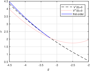
Figure 4: Phase diagram for $p(t)=e^{-t^{3}-gt^{2}-\nu t}$.

The dashed (black) and dotted (red) curves in Figure 4 are respectively the curves defined implicitly by $V^{\prime}(0)=1-M_{0}=0$ and $V^{\prime\prime}(0)=M_{0}^{2}-M_{1}=0$. Above the dashed curve $V^{\prime}(0)>0$ and below the dashed curve $V^{\prime}(0)<0$. Above the dotted curve $V^{\prime\prime}(0)<0$ and below the curve $V^{\prime\prime}(0)>0$. Below the curve $V^{\prime}(0)=0$ there is a unique solution to $V^{\prime}(t_{0})=0$. The two curves $V^{\prime}(0)=0$ and $V^{\prime\prime}(0)=0$ intersect at the tricritical point, which is

$$g_{c}=-3.2103...,\quad\nu_{c}=2.0772...\,.$$ (4.2)

The solid curve (for $g\leq g_{c}$) is the first-order curve and the dashed curve (for $g\geq g_{c}$) is the second-order curve. These two curves satisfy the conditions of Definition 1.2. Together the first- and second-order curves define the phase boundary $\nu_{c}(g)$. Points below the phase boundary are in the dense phase in the sense of Definition 1.2, and points above the phase boundary are in the dilute phase in the sense of Definition 1.2. The first few moments at the tricritical point are

$$M^{c}_{0}=M^{c}_{1}=1,\quad M^{c}_{2}=1.4478...,\quad M^{c}_{3}=2.4062...,\quad M^{c}_{4}=4.3315....$$ (4.3)

To distinguish moments at the tricritical point $(g_{c},\nu_{c})$ from moments computed at other points $(g,\nu)$, we write the former as $M_{i}^{c}$ and the latter simply as $M_{i}$.

4.2 First derivative of phase boundary

We prove Theorem 1.5(i) in two lemmas. Together, the lemmas show that the phase boundary is differentiable but not twice differentiable at the tricritical point with derivative $-M_{2}^{c}$. In this section, we prove the differentiability. The proof of the inequality of the left and right second derivatives at the tricritical point is deferred to Lemma 4.6. Here and throughout Section 4, we use the following elementary facts about derivatives of moments, for $i\geq 0$:

$$M_{i,g}=-M_{i+2},\quad M_{i,\nu}=-M_{i+1},\quad M_{i,gg}=M_{i+4},\quad M_{i,g\nu}=M_{i+3},\quad M_{i,\nu\nu}=M_{i+2}.$$ (4.4)

Lemma 4.1.

(i) The tangent to the curve $M_{0}=1$ (the entire dashed curve in Figure 4, including the second-order curve and the tricritical point) has slope $\nu_{g}=-M_{2}/M_{1}$.
(ii) The tangent to the first-order curve at the tricritical point also has slope $\nu_{c,g}=-M^{c}_{2}/M_{1}^{c}=-M_{2}^{c}$.

Proof.

(i) We write the curve $M_{0}=1$ as $\nu=\nu(g)$. Implicit differentiation of $M_{0}(g,\nu(g))=1$ with respect to $g$, together with (4.4), gives $0=M_{0,g}+M_{0,\nu}\nu_{g}=-M_{2}-M_{1}\nu_{g}$, so $\nu_{g}=-M_{2}/M_{1}$.

(ii) On the first-order curve $\nu=\nu_{c}(g)$ (for $g\leq g_{c}$), by Definition 1.2 there are two solutions to $V(t_{0})=0$: $t_{0}=0$ and a positive $t_{0}>0$, which by definition characterises the first-order curve. At the positive root, $V^{\prime}(t_{0})=0$. At the tricritical point, $t_{0}=0$ and $V(0)=V^{\prime}(0)=V^{\prime\prime}(0)=0$. By continuity, as $g\uparrow g_{c}$ we have $t_{0}\rightarrow 0$. Total derivatives with respect to $g$ are denoted $\mathring{f}=\frac{d}{dg}f$.

We differentiate $V(t_{0}(g,\nu_{c}(g)),g,\nu_{c}(g))=0$ with respect to $g$ and obtain

$$V^{\prime}\mathring{t}_{0}+V_{g}+V_{\nu}\nu_{c,g} =0.$$ (4.5)

For every $g\leq g_{c}$, $V^{\prime}(t_{0}(g,\nu_{c}(g)),g,\nu_{c}(g))=0$, so the first term is constant in $g$ and is equal to zero. Also, $V_{\nu}$ is nonzero on the first-order curve, so $\nu_{c,g}=-V_{g}/V_{\nu}$. We parametrise the first order curve as $(g(s),\nu(s))=(g_{c}-s,\nu_{c}(g_{c}-s))$ for $s\geq 0$. By definition, the slope of the tangent to the first-order curve is $\lim_{s\downarrow 0}\nu_{c,g}$. Also, by definition, by (1.21), and by (4.4), as $s\downarrow 0$ we have

$$\frac{V_{g}}{V_{\nu}}=\frac{v_{g}}{v_{\nu}}\sim\frac{M_{0,g}t_{0}}{M_{0,\nu}t_{0}}=\frac{M_{2}}{M_{1}}\sim M_{2}^{c},$$ (4.6)

where we also used $M_{1}^{c}=1$ and the fact that $t_{0}(g(s),\nu(s))\rightarrow 0$ as $s\downarrow 0$. Therefore, at the tricritical point, $\nu_{c,g}=-M_{2}^{c}$.  

4.3 Susceptibility

We now prove Theorem 1.5(ii). Given a point $(g(0),\nu(0))$ on the second-order curve, or the tricritical point, we fix a vector ${\bf m}=(m_{1},m_{2})$ with base at $(g(0),\nu(0))$, which is nontangential to the second-order curve and pointing into the dilute phase. By Lemma 4.1, ${\bf n}=(M_{2},M_{1})$ is normal to the curve and pointing into the dilute phase, so ${\bf m}\cdot{\bf n}>0$ (moments are evaluated at $(g(0),\nu(0))$). We define a line segment in the dilute phase that starts at our fixed point by

$$(g(s),\nu(s))=(g(0)+sm_{1},\nu(0)+sm_{2})\qquad(s\in[0,1]),$$ (4.7)

and set $\chi(s)=\chi(g(s),\nu(s))$. We set $M_{0}(s)=M_{0}(g(s),\nu(s))$ and define other functions similarly.

By (1.27), the infinite-volume susceptibility in the dilute phase is given by

$$\chi=\frac{1-V^{\prime}(0)}{V^{\prime}(0)}=\frac{M_{0}(s)}{1-M_{0}(s)}.$$ (4.8)

By (4.4) and the chain rule, $M_{0}(s)\sim 1-(M_{2}(0)m_{1}+M_{1}(0)m_{2})s=1-({\bf m}\cdot{\bf n})s$ as $s\downarrow 0$. This gives

$$\chi\sim\frac{1}{({\bf m}\cdot{\bf n})s},$$ (4.9)

which proves that $\chi$ diverges as stated in (1.32).

4.4 Density

The effective potential $V$ is smooth in $(g,\nu)$, has a uniquely attained global minimum at $t=0$ on the second-order curve (with $V(0)=0$), has a uniquely attained global minimum at $t_{0}>0$ in the dense phase (with $V(t_{0})<0$), and attains its global minimum at both $0$ and $t_{0}$ on the first-order curve (with $V(0)=V(t_{0})=0$). By smoothness of $V$, $t_{0}\rightarrow 0$ as the second-order curve or tricritical point is approached. In the dense phase, the density is given by $\rho=\dot{V}(t_{0})$, so as $t_{0}\rightarrow 0$, $\dot{V}(t_{0})\sim\dot{V}^{\prime}(0)t_{0}=M_{1}t_{0}$, and at the tricritical point $M_{1}^{c}=1$.

To prove Theorem 1.5(iii), it therefore suffices to prove the following Propositions 4.2, 4.3 and 4.5 for the asymptotic behaviour of $t_{0}$. The values of the constants $A,B_{i}$ in the propositions are specified in their proofs. The fact that the phase boundary is not twice differentiable at the tricritical point is proved in Lemma 4.6, to complete the proof of Theorem 1.5(i).

Let $(g(0),\nu(0))$ be a given point on the second-order curve, or the tricritical point. We again use the normal ${\bf n}=(M_{2},M_{1})$ which points into the dilute phase. As in (4.7) we fix a vector ${\bf m}=(m_{1},m_{2})$, but now with ${\bf m}\cdot{\bf n}<0$ so that ${\bf m}$ points into the dense phase, and we define a line segment that starts at our given point by

$$(g(s),\nu(s))=(g(0)+sm_{1},\nu(0)+sm_{2})\qquad(s\in[0,1]).$$ (4.10)

We consider the asymptotic behaviour of the density $\rho$ along this segment, as $s\downarrow 0$. Let $M_{i}(s)=M_{i}(g(s),\nu(s))$ for $i=0,1,2,\ldots$. An ingredient in the proofs is the asymptotic formula, as $s\downarrow 0$,

$$M_{i}(s)=M_{i}-(m_{1}M_{i+2}+m_{2}M_{i+1})s+\frac{1}{2}(m_{1}^{2}M_{i+4}+2m_{1}m_{2}M_{i+3}+m_{2}^{2}M_{i+2})s^{2}+O(s^{3}),$$ (4.11)

with all moments on the right-hand side evaluated at $s=0$. This follows from Taylor’s theorem and (4.4).

4.4.1 Approach to second-order curve from dense phase

Proposition 4.2.

As the second-order curve is approached,

$$t_{0}\sim\begin{cases}\frac{|{\bf m}\cdot{\bf n}|}{1-M_{1}}s&\text{(nontangentially from dense phase)}\\ As^{2}&\text{(tangentially from dense phase)}.\end{cases}$$ (4.12)

The constant $A$ is strictly positive at least along some arc of the second-order curve adjacent to the tricritical point.

Proof.

We parametrise the approach to a point $(g(0),\nu(0))$ on the second order curve as $(g(s),\nu(s))$ with $s\downarrow 0$, as in (4.10), and we write $V_{s}(t)=V(g(s),\nu(s);t)$. On the second order curve, $V^{\prime}_{0}(0)=0$, $V^{\prime\prime}_{0}(0)>0$ and $0$ is a global minimum of $V_{0}$. On the other hand, for $s>0$ there is a unique solution $t_{0}=t_{0}(s)>0$ to $V^{\prime}_{s}(t_{0}(s))=0$. The condition $V^{\prime}(t_{0})=0$ is equivalent to $1+v(t_{0})=v^{\prime}(t_{0})$, so

$$1+v(0)+v^{\prime}(0)t_{0}=v^{\prime}(0)+v^{\prime\prime}(0)t_{0}+O(t_{0}^{2}).$$ (4.13)

By (1.21), this gives

$$1+M_{0}t_{0}=M_{0}+M_{1}t_{0}+O(t_{0}^{2}).$$ (4.14)

Therefore, since $t_{0}=o_{s}(1)$, $1-M_{1}(0)>0$, and $M_{0}(s)-1=o_{s}(1)$,

$$t_{0}=\frac{M_{0}-1}{M_{0}-M_{1}}(1+O(t_{0}))\sim\frac{M_{0}-1}{1-M_{1}(0)}.$$ (4.15)

Second-order curve nontangentially from dense phase. By (4.15) and (4.11),

$$t_{0}\sim\frac{|{\bf m}\cdot{\bf n}|}{1-M_{1}(0)}s.$$ (4.16)

This proves the result for the nontangential approach, for which ${\bf m}\cdot{\bf n}<0$.

Second-order curve tangentially from dense phase. For the tangential approach, we choose ${\bf m}=(M_{1},-M_{2})$ so that ${\bf m}\cdot{\bf n}=0$. By (4.11) we have $M_{0}(s)\sim 1+as^{2}$ with $a=\frac{1}{2}(M_{1}^{2}M_{4}-2M_{1}M_{2}M_{3}+M_{2}^{3})$, so now

$$t_{0}\sim\frac{a}{1-M_{1}(0)}s^{2}$$ (4.17)

(all moments are evaluated at $s=0$ here). At the tricritical point, $a^{c}=M_{4}^{c}-2M_{2}^{c}M_{3}^{c}+(M_{2}^{c})^{3}>0$ by (4.3) (cf. Lemma 4.6). By continuity, $a$ remains positive at least along some arc of the second-order curve adjacent to the tricritical point. The constant $A$ is $A=(1-M_{1})^{-1}a$.  

4.4.2 Approach to tricritical point from dense phase

We parametrise the approach to the tricritical point $(g_{c},\nu_{c})$ as $(g(s),\nu(s))$ with $s\downarrow 0$, as in (4.10), and we write $V_{s}(t)=V(g(s),\nu(s);t)$. For both tangential and nontangential approach to the tricritical point from the dense phase, the approach is from below the curve $V^{\prime}(0)=1-M_{0}=0$ and there is one solution $t_{0}=t_{0}(s)>0$ to $V_{s}^{\prime}(t_{0})=0$. An example is depicted in Figure 5. For this approach, $V_{s}^{\prime}(0)=1-M_{0}<0$, and $V_{s}^{\prime\prime}(0)=M_{0}^{2}-M_{1}$ can have either sign or equal zero (the dotted curve in Figure 4 is the curve $V^{\prime\prime}(0)=0$).

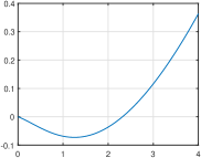
Figure 5: Effective potential $V$ vs $t$ on tangent line (first-order side), at $(g,\nu)=(-3.700,2.786)$. The point $t_{0}$ is the location of the minimum.

Proposition 4.3.

As the tricritical point is approached,

$$t_{0}\sim\begin{cases}B_{0}(|{\bf m}\cdot{\bf n}|s)^{1/2}&\text{(nontangentially from dense phase)}\\ B_{1}s&\text{(tangentially from second-order side)}\\ B_{2}s&\text{(tangentially from first-order side}).\end{cases}$$ (4.18)

The constants $B_{0},B_{1},B_{2}$ are all strictly positive.

The proof of Proposition 4.3 uses the following elementary lemma, which gives an estimate for how fast $t_{0}\rightarrow 0$.

Lemma 4.4.

For $s\in[0,1]$, let $f_{s}:[0,\infty)\rightarrow{\mathbb{R}}$ be smooth functions, with $f_{s}$ and its derivatives uniformly continuous (and hence uniformly bounded) in small $s,t$. Suppose that $f_{0}(0)=f_{0}^{\prime}(0)=0$, $f_{0}^{\prime\prime}(0)>0$, and that $f_{s}(0)<0$ for $s>0$. Then for small $s>0$ there is a unique root $t_{0}=t_{0}(s)$ of $f_{s}(t_{0}(s))=0$ and as $s\downarrow 0$,

$$t_{0}(s)=O(|f_{s}(0)|^{1/2}+|f_{s}^{\prime}(0)|).$$ (4.19)

Proof.

By the assumptions that $f_{0}^{\prime\prime}(0)>0$ and that $f_{s}^{\prime\prime}(t)$ is uniformly continuous in small $s,t$, there are $\delta,c>0$ such that $f_{s}^{\prime\prime}(t)\geq 2c$ for $s,t\leq\delta$, and hence $f_{s}(t)\geq f_{s}(0)+f_{s}^{\prime}(0)t+ct^{2}=-|f_{s}(0)|+f_{s}^{\prime}(0)t+ct^{2}$ for $s,t\leq\delta$. Since the positive roots to $-a+bt+ct^{2}=0$ with $a,c>0$ are

$$t=\frac{1}{2c}(-b+\sqrt{b^{2}+4ac})\leq\frac{1}{2c}(2\max\{-b,0\}+2\sqrt{ac})=\frac{\max\{-b,0\}}{c}+\sqrt{\frac{a}{c}},$$ (4.20)

we see that $f_{s}(t)>0$ if $t>\sqrt{|f_{s}(0)|/c}+\max\{-f_{s}^{\prime}(0),0\}/c$. In particular, for $s$ small enough that $\sqrt{|f_{s}(0)|/c}+|f_{s}^{\prime}(0)|/c\leq\delta$, it follows by continuity and $f_{s}(0)<0$ that $f_{s}$ has a root $t_{0}=t_{0}(s)\in[0,\delta]$ to $f_{s}(t_{0})=0$ satisfying $t_{0}=O(\sqrt{|f_{s}(0)|}+|f^{\prime}_{s}(0)|)$. Since $f_{s}$ is convex on $[0,\delta]$, this root is unique.  

Proof of Proposition 4.3.

We apply Lemma 4.4 to $f_{s}(t)=V^{\prime}_{s}(t)$. The hypotheses are satisfied: $f_{s}(0)=1-M_{0}(s)<0$, $f_{0}^{\prime}(0)=0$, and by (1.17) and (4.3),

$$\alpha=f_{0}^{\prime\prime}(0)=V^{\prime\prime\prime}_{0}(0)=-\frac{1}{2}M_{2}^{c}+1>0.$$ (4.21)

Taylor expansion of $V^{\prime}(t_{0})=0$ gives

$$V^{\prime}(0)+V^{\prime\prime}(0)t_{0}+\frac{1}{2}V^{\prime\prime\prime}(0)t_{0}^{2}+O(t_{0}^{3})=0.$$ (4.22)

It follows from Lemma 4.4 that

$$t_{0} =\frac{-V^{\prime\prime}(0)\pm\sqrt{V^{\prime\prime}(0)^{2}-2V^{\prime\prime\prime}(0)(V^{\prime}(0)+O(|V^{\prime}(0)|^{3/2}+|V^{\prime\prime}(0)|^{3})}}{V^{\prime\prime\prime}(0)}$$ (4.23)

Tricritical point nontangentially from dense phase. By (4.11), in this case we have

$$V_{s}^{\prime}(0)=1-M_{0}(s)\sim-|{\bf m}\cdot{\bf n}|s,\qquad V_{s}^{\prime\prime}(0)\sim 1-M_{1}(s)=O(s).$$ (4.24)

Therefore the error term in (4.23) is $O(s^{3/2})$ and hence

$$t_{0} \sim\alpha^{-1}(2\alpha|{\bf m}\cdot{\bf n}|s)^{1/2}.$$ (4.25)

The constant $B_{0}$ is $B_{0}=(2\alpha^{-1})^{1/2}=2(2-M_{2}^{c})^{-1/2}$.

Tricritical point tangentially from second-order side. The slope of the tangent line at the tricritical point is $-M_{2}^{c}$, so the tangential approach is parametrised by (4.10) with ${\bf m}=(1,-M_{2}^{c})$. On this tangent line, $M_{0}>1$ and $M_{0}^{2}-M_{1}>0$ (see Figure 4). As above (4.17), $M_{0}(s)\sim 1+a^{c}s^{2}$ with $a^{c}=\frac{1}{2}((M_{1}^{c})^{2}M_{4}^{c}-2M_{1}^{c}M_{2}^{c}M_{3}^{c}+(M_{2}^{c})^{3})>0$, and by (4.11) $M_{1}(s)\sim 1-bs$ with $b=M_{3}^{c}-(M_{2}^{c})^{2}>0$ by (4.3). Therefore,

$$V_{s}^{\prime}(0)=1-M_{0}(s)\sim-a^{c}s^{2},\qquad V_{s}^{\prime\prime}(0)=M_{0}(s)^{2}-M_{1}(s)\sim bs.$$ (4.26)

As in the previous case, we apply Lemma 4.4 and (4.23) but this time with an error term which is $O(s^{3})$. This leads to

$$t_{0}\sim\alpha^{-1}\Big{(}-bs+\sqrt{b^{2}s^{2}+2\alpha as^{2}}\Big{)}=\alpha^{-1}\Big{(}-b+\sqrt{b^{2}+2\alpha a}\Big{)}s.$$ (4.27)

The constant $B_{1}$ is $B_{1}=\alpha^{-1}(-b+\sqrt{b^{2}+2\alpha a})>0$.

Tricritical point tangentially from first-order side. Now we parametrise the tangential approach as in (4.10) with ${\bf m}=(-1,M_{2}^{c})$. Now $M_{0}>1$ and $M_{0}^{2}-M_{1}<0$ (see Figure 4). The formula (4.23) again applies with error term $O(s^{3})$. Again $M_{0}(s)\sim 1+as^{2}$, but now

$$M_{1}(s)\sim 1+bs$$ (4.28)

due to the replacement of ${\bf m}$ by $-{\bf m}$. Therefore,

$$t_{0}\sim\alpha^{-1}\Big{(}bs+\sqrt{b^{2}s^{2}+2\alpha as^{2}}\Big{)}=\alpha^{-1}\Big{(}b+\sqrt{b^{2}+2\alpha a}\Big{)}s.$$ (4.29)

The constant $B_{2}$ is $B_{2}=\alpha^{-1}(b+\sqrt{b^{2}+2\alpha a})>0$.  

4.4.3 Approach to tricritical point along first-order curve

We now complete the proof of Theorem 1.5, by proving the last case of Theorem 1.5(iii) in Proposition 4.5 and the remaining part of Theorem 1.5(i) (namely the failure of the phase boundary to be twice differentiable) in Lemma 4.6. The focus is on the location $t_{0}$ of the nonzero minimum of the effective potential on the first-order curve. Figure 6 shows a typical $V$.

Figure 6: Effective potential $V$ vs $t$ on first-order curve, at $(g,\nu)=(-3.700,2.864)$. The point $t_{0}$ is the unique positive solution to $V(t_{0})=0$.

Proposition 4.5.

As the tricritical point is approached along the first-order curve $(g(s),\nu(s))=(g_{c}-s,\nu_{c}(g_{c}-s))$,

$$t_{0}\sim B_{3}s\qquad\text{(along first-order curve}).$$ (4.30)

The constant $B_{3}$ is strictly positive.

Proof.

On the first-order curve, $V_{s}^{\prime}(0)>0$ and $V_{s}^{\prime\prime}(0)<0$ (see Figure 4), and there is a unique $t_{0}>0$ such that $V_{s}(t_{0})=0$. At this minimum, $V_{s}^{\prime}(t_{0})=0$ and $V_{s}^{\prime\prime}(t_{0})>0$. Under Taylor expansion, together with the fact that $V_{s}(0)=0$, the equations $V_{s}(t_{0})=0$ and $V_{s}^{\prime}(t_{0})=0$ become

$$0 =t_{0}\left(V_{s}^{\prime}(0)+\frac{1}{2!}V_{s}^{\prime\prime}(0)t_{0}+\frac{1}{3!}V_{s}^{\prime\prime\prime}(0)t_{0}^{2}+O(t_{0}^{3})\right)$$ (4.31)

$$0 =V_{s}^{\prime}(0)+V_{s}^{\prime\prime}(0)t_{0}+\frac{1}{2!}V_{s}^{\prime\prime}(0)t_{0}^{2}+O(t_{0}^{3}).$$ (4.32)

By the chain rule, $\frac{d}{ds}\nu_{c}(g(s))=-\nu_{c,g}(g(s))$, and by Lemma 4.1, $-\nu_{c,g}(g(s))\rightarrow M_{2}^{c}$ as $s\downarrow 0$. Therefore, as in (4.28),

$$M_{1}(s)\sim 1+bs,$$ (4.33)

with $b=M_{3}^{c}-(M_{2}^{c})^{2}>0$. Also, since

$$\frac{d}{ds}M_{0}(s) =-M_{0,g}(s)-M_{0,\nu}(s)\nu_{c}^{\prime}(g_{c}-s)\rightarrow M_{2}^{c}-M_{1}^{c}(-M_{2}^{c}/M_{1}^{c})=0\qquad(s\rightarrow 0),$$ (4.34)

it follows that

$$V_{s}^{\prime\prime}(0)=M_{0}(s)^{2}-M_{1}(s)\sim-bs.$$ (4.35)

We substitute this into (4.31)–(4.32) and use $V^{\prime\prime\prime}(0)=\alpha=1-\frac{1}{2}M_{2}^{c}>0$, to find that

$$V^{\prime}(0)-\frac{bs}{2}t_{0}+\frac{\alpha}{6}t_{0}^{2}=O(t_{0}(t_{0}+s)^{2}),$$ (4.36)

$$V^{\prime}(0)-bst_{0}+\frac{\alpha}{2}t_{0}^{2}=O(t_{0}(t_{0}+s)^{2}),$$ (4.37)

and hence

$$V^{\prime}(0)-\frac{bs}{4}t_{0}=O(t_{0}(t_{0}+s)^{2}).$$ (4.38)

We substitute (4.38) into either of (4.31)–(4.32), and after cancellation of a factor $t_{0}$, we obtain

$$-\frac{bs}{4}+\frac{\alpha}{6}t_{0}=O(t_{0}+s)^{2}.$$ (4.39)

Since $t_{0}=o_{s}(1)$, this gives

$$t_{0}\sim\frac{3b}{2\alpha}s=B_{3}s,$$ (4.40)

so $B_{3}=\frac{3b}{2\alpha}=3\frac{M_{3}^{c}-(M_{2}^{c})^{2}}{2-M_{2}^{c}}>0$ and the proof is complete.  

Note that the conclusion (4.30) agrees with the naive argument (ignoring the error term) that the quadratic in (4.31) will have a unique root precisely when the discriminant vanishes, i.e., when

$$V_{s}^{\prime}(0)=\frac{3}{8}\frac{V_{s}^{\prime\prime}(0)^{2}}{V_{s}^{\prime\prime\prime}(0)},$$ (4.41)

and in this case the root is $t_{0}=\frac{3}{2}\frac{|V_{s}^{\prime\prime}(0)|}{V_{s}^{\prime\prime\prime}(0)}\sim\frac{3}{2}\frac{bs}{\alpha}$.

Finally, we prove the remaining part of Theorem 1.5(iii), concerning the behaviour of the density as the tricritical point is approached along the first-order curve.

Lemma 4.6.

(i) At the tricritical point, the second derivative of the second-order curve is given by $\nu_{gg}=M_{4}^{c}-2M_{3}^{c}M_{2}^{c}+(M_{2}^{c})^{3}>0$.
(ii) At the tricritical point, the second derivative of the first-order curve is instead $\nu_{c,gg}=M_{4}^{c}-2M_{3}^{c}M_{2}^{c}+(M_{2}^{c})^{3}+3b^{2}/(4\alpha)$, with $b=M_{3}^{c}-(M_{2}^{c})^{2}>0$ and with $\alpha=1-\frac{1}{2}M_{2}^{c}>0$.

Proof.

(i) The second-order curve $\nu=\nu(g)$ is given by $V^{\prime}(0)=0$. Since $V^{\prime}(0)=1-M_{0}$, a first differentiation with respect to $g$ gives $0=M_{0,g}+M_{0,\nu}\nu_{g}$, and a second differentiation gives

$$0 =M_{0,gg}+2M_{0,\nu g}\nu_{g}+M_{0,\nu\nu}\nu_{g}^{2}+M_{0,\nu}\nu_{gg}.$$ (4.42)

We use $\nu_{g}=-M_{2}/M_{1}$ from Lemma 4.1(i), (4.4), and $M_{1}^{c}=1$ to see that, at the tricritical point,

$$\nu_{c,gg}=M_{4}^{c}-2M_{3}^{c}M_{2}^{c}+(M_{2}^{c})^{3}.$$ (4.43)

By (4.3), $\nu_{c,gg}>0$.

(ii) By (4.5), on the first-order curve we have $V_{g}+V_{\nu}\nu_{c,g}=0$. Total derivatives with respect to $g$ are denoted $\mathring{f}=\frac{d}{dg}f$. Differentiation with respect to $g$ gives

$$\mathring{V}_{g}+\mathring{V}_{\nu}\nu_{c,g}+V_{\nu}\nu_{c,gg} =0,$$ (4.44)

so, since $V_{\nu}\sim M_{1}^{c}t_{0}=t_{0}$ by (1.21),

$$\nu_{c,gg}=-\frac{1}{V_{\nu}}(\mathring{V}_{g}+\mathring{V}_{\nu}\nu_{c,g})\sim-\frac{1}{t_{0}}(\mathring{V}_{g}+\mathring{V}_{\nu}\nu_{c,g}).$$ (4.45)

We need to compute the coefficient of $t_{0}$ in $\mathring{V}_{g}+\mathring{V}_{\nu}\nu_{c,g}$. Since

$$\mathring{V}_{g} =V_{g}^{\prime}\mathring{t}_{0}+V_{gg}+V_{g\nu}\nu_{c,g},$$ (4.46)

$$\mathring{V}_{\nu} =V_{\nu}^{\prime}\mathring{t}_{0}+V_{\nu g}+V_{\nu\nu}\nu_{c,g},$$ (4.47)

we obtain

$$\nu_{c,gg}\sim-\frac{1}{t_{0}}\left((V_{g}^{\prime}+V_{\nu}^{\prime}\nu_{c,g})\mathring{t}_{0}+V_{gg}+V_{\nu g}\nu_{c,g}+(V_{g\nu}+V_{\nu\nu}\nu_{c,g})\nu_{c,g}\right).$$ (4.48)

From (1.21),

$$V_{gg}=-\frac{v_{gg}}{1+v}+\frac{v_{g}^{2}}{(1+v)^{2}}\sim-v_{gg}+O(t_{0}^{2})\sim-M_{0,gg}t_{0}\sim-M_{4}^{c}t_{0}.$$ (4.49)

Similarly, $V_{g\nu}\sim-M_{3}^{c}t_{0}$ and $V_{\nu\nu}\sim-M_{2}^{c}t_{0}$. Therefore, since $\nu_{c,g}\sim-M_{2}^{c}$ by Lemma 4.1(ii), and since $-\mathring{t}_{0}\rightarrow B_{3}=\frac{3b}{2\alpha}$ as $g\uparrow g_{c}$ by Proposition 4.5,

$$\nu_{c,gg}\sim\left(M_{4}^{c}-2M_{2}^{c}M_{3}^{c}+(M_{2}^{c})^{3}\right)+B_{3}\frac{1}{t_{0}}(V_{g}^{\prime}+V_{\nu}^{\prime}\nu_{c,g}).$$ (4.50)

Let $f(g)=V_{g}^{\prime}+V_{\nu}^{\prime}\nu_{c,g}$. Since $f(g_{c})=M_{2}^{c}+M_{1}^{c}(-M_{2}^{c})=0$, we need the next order term. Direct computation gives

$$V_{g}^{\prime}+V_{\nu}^{\prime}\nu_{c,g} =\frac{1}{(1+v)^{2}}\left(-v_{g}^{\prime}(1+v)+v^{\prime}v_{g}-(-v^{\prime}_{\nu}(1+v)+v^{\prime}v_{\nu})\frac{v_{g}}{v_{\nu}}\right).$$ (4.51)

By (1.21) and (4.4), together with $M_{0}^{c}=M_{1}^{c}=1$

$$v =M_{0}t+\frac{1}{2}M_{1}t^{2}+\cdots\sim t+\frac{1}{2}t^{2}+\cdots,$$ (4.52)

$$v^{\prime} =M_{0}+M_{1}t+\cdots\sim 1+t+\cdots,$$ (4.53)

$$v_{g} =M_{0,g}t+\frac{1}{2}M_{1,g}t^{2}+\cdots\sim-M_{2}^{c}t-\frac{1}{2}M_{3}^{c}t^{2}+\cdots,$$ (4.54)

$$v_{\nu} =M_{0,\nu}t+\frac{1}{2}M_{1,\nu}t^{2}+\cdots\sim-t-\frac{1}{2}M_{2}^{c}t^{2}+\cdots,$$ (4.55)

$$v_{g}^{\prime} \sim-M_{2}^{c}-M_{3}^{c}t,$$ (4.56)

$$v_{\nu}^{\prime} \sim-1-M_{2}^{c}t.$$ (4.57)

Therefore,

$$V_{g}^{\prime}+V_{\nu}^{\prime}\nu_{c,g} \sim(M_{2}^{c}+M_{3}^{c}t)(1+t)-M_{2}t-((1+M_{2}^{c}t)(1+t)-t)\frac{M_{2}^{c}+\frac{1}{2}M_{3}^{c}t}{1+\frac{1}{2}M_{2}^{c}t}$$

$$\sim M_{2}^{c}+M_{3}^{c}t-(1+M_{2}t)(M_{2}^{c}+\frac{1}{2}M_{3}^{c}t)(1-\frac{1}{2}M_{2}^{c}t)$$

$$\sim\frac{1}{2}(M_{3}^{c}-(M_{2}^{c})^{2})t=\frac{b}{2}t,$$ (4.58)

and the proof is complete.

References

- [1] D. Arovas. Lecture notes on thermodynamics and statistical mechanics. In preparation. https://courses.physics.ucsd.edu/2017/Spring/physics210a/LECTURES/BOOK_STATMECH.pdf, (2019). Accessed May 8, 2020.
- [2] R. Bauerschmidt, D.C. Brydges, and G. Slade. Introduction to a Renormalisation Group Method. Lecture Notes in Mathematics Vol. 2242. Springer Nature, Singapore, (2019).
- [3] R. Bauerschmidt, M. Lohmann, and G. Slade. Three-dimensional tricritical spins and polymers. J. Math. Phys., 61:033302, (2020).
- [4] R. Bauerschmidt, G. Slade, and B.C. Wallace. Four-dimensional weakly self-avoiding walk with contact self-attraction. J. Stat. Phys, 167:317–350, (2017).
- [5] M. Bousquet-Mélou, A.J. Guttmann, and I. Jensen. Self-avoiding walks crossing a square. J. Phys. A: Math. Gen., 38:9158–9181, (2005).
- [6] D.C. Brydges and J.Z. Imbrie. Green’s function for a hierarchical self-avoiding walk in four dimensions. Commun. Math. Phys., 239:549–584, (2003).
- [7] Y. Deng, T.M. Garoni, J. Grimm, A. Nasrawi and Z. Zhou. The length of self-avoiding walks on the complete graph. J. Stat. Mech: Theory Exp., 103206, (2019).
- [8] H. Duminil-Copin, G. Kozma, and A. Yadin. Supercritical self-avoiding walks are space-filling. Ann. Inst. H. Poincaré Probab. Statist., 50:315–326, (2014).
- [9] B. Duplantier. Tricritical polymer chains in or below three dimensions. Europhys. Lett., 1:491–498, (1986).
- [10] B. Duplantier. Geometry of polymer chains near the theta-point and dimensional regularization. J. Chem. Phys., 86:4233–4244, (1987).
- [11] B. Duplantier and H. Saleur. Exact critical properties of two-dimensional dense self-avoiding walks. Nucl. Phys. B, 290 [FS20]:291–326, (1987).
- [12] B. Duplantier and H. Saleur. Exact tricritical exponents for polymers at the point in two dimensions. Phys. Rev. Lett., 59:539–542, (1987).
- [13] P.G. de Gennes. Scaling Concepts in Polymer Physics. Cornell University Press, Ithaca, (1979).
- [14] S.E. Golowich and J.Z. Imbrie. The broken supersymmetry phase of a self-avoiding random walk. Commun. Math. Phys., 168:265–319, (1995).
- [15] A. Hammond and T. Helmuth. Self-attracting self-avoiding walk. Probab. Theory Related Fields, 175:677–719, (2019).
- [16] F. den Hollander. Random Polymers. Springer, Berlin, (2009). Lecture Notes in Mathematics Vol. 1974. Ecole d’Eté de Probabilités de Saint–Flour XXXVII–2007.
- [17] N. Madras. Critical behaviour of self-avoiding walks that cross a square. J. Phys. A: Math. Gen., 28:1535–1547, (1995).
- [18] F.W.J. Olver. Why steepest descents? SIAM Review, 12:228–247, (1970).
- [19] F.W.J. Olver. Asymptotics and Special Functions. CRC Press, New York, (1997).
- [20] N. Pétrélis and N. Torri. Collapse transition of the interacting prudent walk. Ann. Inst. Henri Poincaré Comb. Phys. Interact., 5:387–435, (2018).
- [21] G. Slade. Self-avoiding walk on the complete graph. To appear in J. Math. Soc. Japan. Advance online publication (2020): https://doi.org/10.2969/jmsj/82588258.