Generalized Scharfetter–Gummel schemes for electro-thermal transport in degenerate semiconductors using the Kelvin formula for the Seebeck coefficient

Abstract

Many challenges faced in today’s semiconductor devices are related to self-heating phenomena. The optimization of device designs can be assisted by numerical simulations using the non-isothermal drift-diffusion system, where the magnitude of the thermoelectric cross effects is controlled by the Seebeck coefficient. We show that the model equations take a remarkably simple form when assuming the so-called Kelvin formula for the Seebeck coefficient. The corresponding heat generation rate involves exactly the three classically known self-heating effects, namely Joule, recombination and Thomson–Peltier heating, without any further (transient) contributions. Moreover, the thermal driving force in the electrical current density expressions can be entirely absorbed in the diffusion coefficient via a generalized Einstein relation. The efficient numerical simulation relies on an accurate and robust discretization technique for the fluxes (finite volume Scharfetter–Gummel method), which allows to cope with the typically stiff solutions of the semiconductor device equations. We derive two non-isothermal generalizations of the Scharfetter–Gummel scheme for degenerate semiconductors (Fermi–Dirac statistics) obeying the Kelvin formula. The approaches differ in the treatment of degeneration effects: The first is based on an approximation of the discrete generalized Einstein relation implying a specifically modified thermal voltage, whereas the second scheme follows the conventionally used approach employing a modified electric field. We present a detailed analysis and comparison of both schemes, indicating a superior performance of the modified thermal voltage scheme.

200mm(17.5mm,266mm) © 2019. Licensed under the Creative Commons CC-BY-NC-ND 4.0.

1 Introduction

Thermal effects cause many challenges in a broad variety of semiconductor devices. Thermal instabilities limit the safe-operating area of high power devices and modules in electrical energy technology [1, 2], electro-thermal feedback loops lead to catastrophic snapback phenomena in organic light-emitting diodes [3, 4] and self-heating effects decisively limit the achievable output power of semiconductor lasers [5, 6, 7, 8]. The numerical simulation of semiconductor devices showing strong self-heating and thermoelectric effects requires a thermodynamically consistent modeling approach, that describes the coupled charge carrier and heat transport processes. In the context of semiconductor device simulation, the non-isothermal drift-diffusion system [9, 10, 11, 12, 13, 14] has become the standard model for the self-consistent description of electro-thermal transport phenomena. This is a system of four partial differential equations, which couples the semiconductor device equations [15, 16] to a (lattice) heat flow equation for the temperature distribution in the device. On the step from the isothermal to the non-isothermal drift-diffusion system, additional thermoelectric transport coefficients must be included in the theory. The magnitude of the thermoelectric cross-effects is governed by the Seebeck coefficient (also thermopower), which quantifies the thermoelectric voltage induced by a temperature gradient (Seebeck effect) [17, 18]. The reciprocal phenomenon of the Seebeck effect is the Peltier effect, which describes the current-induced heating or cooling at material junctions. As a consequence of Onsager’s reciprocal relations, the Seebeck and Peltier coefficients are not independent such that only the Seebeck coefficient must be specified [19]. Over the decades, several definitions have been proposed for the Seebeck coefficient [20, 21, 22, 23]; recent publications list at least five coexisting different (approximate) formulas [24, 25]. In the context of semiconductor device simulation, the Seebeck coefficients are typically derived from the Boltzmann transport equation in relaxation time approximation [26, 27, 28] or defined according to the adage of the Seebeck coefficient being the “(specific) entropy per carrier” [13, 14, 18, 29]. These approaches are often focused on non-degenerate semiconductors, where the carriers follow the classical Maxwell–Boltzmann statistics. This approximation breaks down in heavily doped semiconductors, where the electron-hole plasma becomes degenerate and Fermi–Dirac statistics must be considered to properly take into account the Pauli exclusion principle. Degeneration effects are important in many semiconductor devices such as semiconductor lasers, light emitting diodes or transistors. Moreover, heavily doped semiconductors are considered as “good” thermoelectric materials, i. e., materials with high thermoelectric figure of merit [17, 18], for thermoelectric generators, which can generate electricity from waste heat [30, 31].

In this paper, we will consider an alternative model for the Seebeck coefficient, which is the so-called Kelvin formula for the thermopower [32]. The Kelvin formula recently gained interest in theoretical condensed matter physics and has been shown to yield a good approximation of the Seebeck coefficient for many materials (including semiconductors, metals and high temperature superconductors) at reasonably high temperatures [33, 34, 32, 35, 36, 37, 38, 39, 40, 41, 42]. The Kelvin formula relates the Seebeck coefficient to the derivative of the entropy density with respect to the carrier density and therefore involves only equilibrium properties of the electron-hole plasma, where degeneration effects are easily included. To our knowledge, the Kelvin formula has not been considered in the context of semiconductor device simulation so far. In Sec. 2, we show that the Kelvin formula yields a remarkably simple form of the non-isothermal drift-diffusion system, which shows two exceptional features:

1. The heat generation rate involves exactly the three classically known self-heating effects (Joule, Thomson–Peltier and recombination heating) without any further (transient) contributions.

2. The thermal driving force in the current density expressions can be entirely absorbed in a (nonlinear) diffusion coefficient via a generalized Einstein relation. Hence, the $\nabla T$ term is eliminated in the drift-diffusion form.

The second part of this paper (Sec. 3) deals with the discretization of the electrical current density expressions, which are required in (non-isothermal) semiconductor device simulation tools. The robust and accurate discretization of the drift-diffusion fluxes in semiconductors with exponentially varying carrier densities is a non-trivial problem, that requires a special purpose discretization technique. The problem has been solved by Scharfetter and Gummel for the case of non-degenerate semiconductors under isothermal conditions [43]. Since then, several adaptations of the method have been developed to account for more general situations (non-isothermal conditions [44, 45, 46, 47, 48, 49, 50, 51], degeneration effects [52, 53, 54, 55, 56, 57]). The Kelvin formula for the Seebeck coefficients allows for a straightforward generalization of the Scharfetter–Gummel approach to the non-isothermal case. We take up two different approaches to incorporate degeneration effects into the non-isothermal Scharfetter–Gummel formula and give an extensive numerical and analytical comparison of both methods. This includes an investigation of limiting cases and structure preserving properties of the discrete formulas (Sec. 3.3), a comparison with the numerically exact solution of the underlying two-point boundary value problem (Sec. 3.4) and a comparison of analytical error bounds (Sec. 3.5). Finally, in Sec. 3.6, we present a numerical convergence analysis of both schemes based on numerical simulations of a one-dimensional p-n-diode.

2 The non-isothermal drift-diffusion system using the Kelvin formula for the Seebeck coefficient

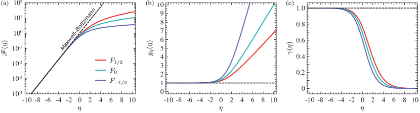
Figure 1: (a) Fermi–Dirac integrals (7) of order $\nu=1/2$, $0$ and $-1/2$ as functions of the reduced Fermi energy $\eta$. For $\eta\ll-1$ the Fermi–Dirac integrals approach the Maxwell–Boltzmann distribution $\mathscr{F}\left(\eta\right)=\exp{\left(\eta\right)}$ (non-degenerate limit). (b) Plot of the degeneracy factor (17b) (or diffusion enhancement factor) for the Fermi–Dirac integrals in (a). For $\eta\ll-1$ the degeneracy factor approaches $1$ (linear diffusion). (c) Correction factor (32) that quantifies the deviation of the Fermi–Dirac integrals from the exponential function. The non-degenerate limit corresponds to $\gamma\left(\eta\right)\equiv 1$.

In this section we briefly review the non-isothermal drift-diffusion system, which provides a self-consistent description of the coupled electro-thermal transport processes in semiconductor devices. The model has been extensively studied by several authors from the perspective of physical kinetics or phenomenological non-equilibrium thermodynamics [9, 10, 11, 12, 13, 14]. The model equations read:

$$-\nabla\cdot\varepsilon\nabla\phi =q\left(C+p-n\right),$$ (1)

$$\partial_{t}n-\frac{1}{q}\nabla\cdot\mathbf{j}_{n} =-R,$$ (2)

$$\partial_{t}p+\frac{1}{q}\nabla\cdot\mathbf{j}_{p} =-R,$$ (3)

$$c_{V}\partial_{t}T-\nabla\cdot\kappa\nabla T =H.$$ (4)

Poisson’s equation (1) describes the electrostatic field generated by the electrical charge density $\rho=q\left(C+p-n\right)$. Here, $\phi$ is the electrostatic potential, $n$ and $p$ are the densities of electrons and holes, respectively, $C$ is the built-in doping profile, $q$ is the elementary charge and $\varepsilon$ is the (absolute) dielectric constant of the material. The transport and recombination dynamics of the electron-hole plasma are modeled by the continuity equations (2)–(3), where $\mathbf{j}_{n/p}$ are the electrical current densities and $R$ is the (net-)recombination rate. The latter includes several radiative and non-radiative recombination processes (Shockley–Read–Hall recombination, Auger recombination, spontaneous emission etc.) [15]. The carrier densities $n$, $p$ are connected with the electrostatic potential $\phi$ via the state equations

$$n =N_{c}\left(T\right)\mathscr{F}\left(\frac{\mu_{c}+q\phi-E_{c}\left(T\right)}{k_{B}T}\right), p =N_{v}\left(T\right)\mathscr{F}\left(\frac{E_{v}\left(T\right)-q\phi-\mu_{v}}{k_{B}T}\right),$$ (5)

where $k_{B}$ is Boltzmann’s constant, $T$ is the absolute temperature, $N_{c/v}$ is the effective density of states and $E_{c/v}$ is the reference energy level (typically the band edge energy) of the conduction band or valence band, respectively. The function $\mathscr{F}$ describes the occupation of the electronic states under quasi-equilibrium conditions, which is controlled by the quasi-Fermi energies $\mu_{c/v}$ of the respective bands. The quasi-Fermi energies are connected with the quasi-Fermi potentials $\varphi_{n/p}$ via

$$\mu_{c} =-q\varphi_{n}, \mu_{v} =-q\varphi_{p}.$$ (6)

In non-degenerate semiconductors (Maxwell–Boltzmann statistics), $\mathscr{F}$ is the exponential function $\mathscr{F}\left(\eta\right)=\exp{\left(\eta\right)}$. Taking the degeneration of the electron-hole plasma due to Pauli-blocking into account (Fermi–Dirac statistics), $\mathscr{F}$ is typically given by the Fermi–Dirac integral

$$\mathscr{F}\left(\eta\right)=F_{\nu}\left(\eta\right)=\frac{1}{\Gamma\left(\nu+1\right)}\int_{0}^{\infty}\mathrm{d}\xi\,\frac{\xi^{\nu}}{\exp{\left(\xi-\eta\right)}+1},$$ (7)

where the index $\nu$ depends on the dimensionality of the structure. Isotropic, bulk materials with parabolic energy bands are described by $\nu=1/2$; for two-dimensional materials (quantum wells) the index $\nu=0$ applies. See Fig. 1 (a) for a plot of the Fermi–Dirac integrals for different $\nu$ as a function of the reduced Fermi energy. The function $\mathscr{F}$ may also include non-parabolicity effects, see Appendix A. In the case of organic semiconductors, $\mathscr{F}$ is often taken as the Gauss–Fermi integral [58, 59] or a hypergeometric function [60, 61].

The heat transport equation (4) describes the spatio-temporal dynamics of the temperature distribution in the device. Here, $c_{V}$ is the (volumetric) heat capacity, $\kappa$ is the thermal conductivity and $H$ is the heat generation rate. The non-isothermal drift-diffusion model assumes a local thermal equilibrium between the lattice and the carriers, i. e., $T=T_{L}=T_{n}=T_{p}$. The system (1)–(4) must be supplemented with initial conditions and boundary conditions (i.e., for electrical contacts, semiconductor-insulator interfaces, heat sinks etc). We refer to Refs. [15, 62] for a survey on commonly used boundary condition models.

The electrical current densities are driven by the gradients of the quasi-Fermi potentials and the temperature

$$\mathbf{j}_{n} =-\sigma_{n}\left(\nabla\varphi_{n}+P_{n}\nabla T\right), \mathbf{j}_{p} =-\sigma_{p}\left(\nabla\varphi_{p}+P_{p}\nabla T\right),$$ (8)

where $\sigma_{n}=qM_{n}n$ and $\sigma_{p}=qM_{p}p$ are the electrical conductivities (with carrier mobilities $M_{n/p}$) and $P_{n/p}$ are the Seebeck coefficients. Finally, we consider a (net-)recombination rate of the form [63]

$$R=R\left(\phi,\varphi_{n},\varphi_{p},T\right)=\left(1-\exp{\left(-\frac{\mu_{c}-\mu_{v}}{k_{B}T}\right)}\right)\sum_{\alpha}r_{\alpha}\left(\phi,\varphi_{n},\varphi_{p},T\right),$$ (9)

which combines several radiative and non-radiative recombination processes labeled by $\alpha$ (e.g., Shockley–Read–Hall recombination, spontaneous emission, Auger recombination etc.). The functions $r_{\alpha}=r_{\alpha}\left(\phi,\varphi_{n},\varphi_{p},T\right)\geq 0$ are inherently non-negative and specific for the respective processes. We refer to Refs. [15, 62] for commonly considered recombination rate models.

2.1 Kelvin formula for the Seebeck coefficient

In this paper, we consider the so-called Kelvin formula for the Seebeck coefficient [32]

$$P_{n} =-\frac{1}{q}\frac{\partial s\left(n,p,T\right)}{\partial n}, P_{p} =+\frac{1}{q}\frac{\partial s\left(n,p,T\right)}{\partial p},$$ (10)

which relates the thermoelectric powers to the derivatives of the entropy density $s=s(n,p,T)$ with respect to the carrier densities. The expression for the entropy density is easily derived from the free energy density $f\left(n,p,T\right)$ of the system, which is a proper thermodynamic potential if the set of unknowns is chosen as $\left(n,p,T\right)$ (“natural variables”) . The expressions for the quasi-Fermi energies and the entropy density then follow as

$$\frac{\partial f\left(n,p,T\right)}{\partial n} =+\mu_{c}\left(n,p,T\right), \frac{\partial f\left(n,p,T\right)}{\partial p} =-\mu_{v}\left(n,p,T\right), \frac{\partial f\left(n,p,T\right)}{\partial T} =-s\left(n,p,T\right).$$ (11)

Taking the second derivatives, this yields the Maxwell relations

$$\frac{\partial\mu_{c}\left(n,p,T\right)}{\partial T} =-\frac{\partial s\left(n,p,T\right)}{\partial n}, \frac{\partial\mu_{v}\left(n,p,T\right)}{\partial T} =+\frac{\partial s\left(n,p,T\right)}{\partial p},$$ (12)

which allow for an alternative representation of Eq. (10). The free energy density includes contributions from the quasi-free electron-hole plasma (ideal Fermi gas), the lattice vibrations (ideal Bose gas) and the electrostatic (Coulomb) interaction energy. Throughout this paper, we assume a free energy density of the form [13]

$$f\left(n,p,T\right)=f_{\text{e--h}}\left(n,p,T\right)+f_{L}\left(T\right)+f_{\text{Coul}}\left(p-n\right).$$ (13)

The free energy density of the (non-interacting) electron-hole plasma reads [13, 63]

$$\begin{aligned} f_{\text{e--h}}\left(n,p,T\right)&=k_{B}T\mathscr{F}^{-1}\left(\frac{n}{N_{c}\left(T\right)}\right)n-k_{B}TN_{c}\left(T\right)\mathscr{G}\left(\mathscr{F}^{-1}\left(\frac{n}{N_{c}\left(T\right)}\right)\right)+E_{c}\left(T\right)n\\ &\hphantom{=}+k_{B}T\mathscr{F}^{-1}\left(\frac{p}{N_{v}\left(T\right)}\right)p-k_{B}TN_{v}\left(T\right)\mathscr{G}\left(\mathscr{F}^{-1}\left(\frac{p}{N_{v}\left(T\right)}\right)\right)-E_{v}\left(T\right)p,\end{aligned}$$ (14)

where $\mathscr{F}^{-1}$ is the inverse of the function $\mathscr{F}$ in the state equations (5) and $\mathscr{G}$ denotes its antiderivative: $\mathscr{G}^{\prime}\left(\eta\right)=\mathscr{F}\left(\eta\right)$. Note that Eq. (14) implies

$$\frac{\partial f_{\text{e--h}}}{\partial n} =k_{B}T\mathscr{F}^{-1}\left(\frac{n}{N_{c}\left(T\right)}\right)+E_{c}\left(T\right), \frac{\partial f_{\text{e--h}}}{\partial p} =k_{B}T\mathscr{F}^{-1}\left(\frac{p}{N_{v}\left(T\right)}\right)-E_{v}\left(T\right).$$ (15a)

The lattice contribution $$f_{L}\left(T\right) c_{V} f_{\text{Coul}} f_{\text{Coul}}$$ yields the dominant contribution to the heat capacity . It can be derived from, e. g., the Debye model for the free phonon gas [64]. The Coulomb interaction energy must be modeled such that the state equations (5) follow consistently from solving the defining relations for the quasi-Fermi energies (11) for the carrier densities. In order to supplement the “missing” electrostatic contributions in Eq. (15a), we specify the derivatives of with respect to the carrier densities:

$$\frac{\partial f_{\text{Coul}}}{\partial n} =-q\phi, \frac{\partial f_{\text{Coul}}}{\partial p} =+q\phi.$$ (15b)

We refer to Albinus et al. [13] for a rigorous mathematical treatment of the Coulomb interaction energy.

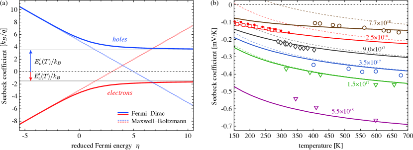
Figure 2: (a) Seebeck coefficient according to the Kelvin formula (16) as a function of the reduced Fermi energy $\eta$ for power law type effective density of states $N_{c/v}\propto T^{3/2}$ and $\mathscr{F}\left(\eta\right)=F_{1/2}\left(\eta\right)$ in units of $k_{B}/q$. The formula (16) takes degeneration effects (Fermi–Dirac statistics, solid lines) of the electron-hole plasma into account, which causes a deviation from the non-degenerate result (Maxwell–Boltzmann statistics, dashed lines) at $\eta\gtrsim-1$. The temperature dependency of the band gap energy yields an offset of $E_{c}^{\prime}\left(T\right)=\left(\chi+\frac{1}{2}\right)E_{g}^{\prime}\left(T\right)$ for electrons (red lines) and $E_{v}^{\prime}=\left(\chi-\frac{1}{2}\right)E_{g}^{\prime}\left(T\right)$ for holes (blue lines). The plot is for $\chi=-0.2$ and $k_{B}^{-1}E_{g}^{\prime}\left(T\right)=-5$. (b) Seebeck coefficient for n-type GaAs. Solid lines are computed according to the Kelvin formula (16a) using Fermi–Dirac statistics, dashed lines indicate the corresponding non-degenerate limit. The respective ionized donor densities $C=N_{D}^{+}$ are given in the plot in units of $\text{cm}^{-3}$. The temperature-dependency of the band gap energy $E_{g}\left(T\right)$ is modeled by the Varshni model (18) with data from Ref. [62] and the effective mass is $m_{c}^{\ast}\left(T\right)=\left(0.067-1.2\times 10^{-5}\,\text{K}^{-1}\,T\right)m_{0}$ [62], where $m_{0}$ is the free electron mass. The fitting parameter is set to $\chi=-0.2$. Experimental data: $\triangledown$ Carlson et al. [65], $\Circle$ Amith et al. [66], $\lozenge$ Edmond et al. [67] (data from Ref. [68]), $\square$ Homm et al. [69] and $\bullet$ Emel’yanenko et al. [70] (data from Ref. [68]).

The Seebeck coefficients (10) are evaluated using Eqs. (11)–(15). Since $f_{\text{Coul}}$ is independent of the temperature and $f_{L}$ does not depend on the carrier densities, the evaluation of Eq. (10) requires only the Maxwell relations (12) and the derivatives of Eqs. (15a) with respect to the temperature. One obtains

$$P_{n}\left(n,T\right) =-\frac{k_{B}}{q}\left(\frac{TN_{c}^{\prime}\left(T\right)}{N_{c}\left(T\right)}g\left(\frac{n}{N_{c}\left(T\right)}\right)-\mathscr{F}^{-1}\left(\frac{n}{N_{c}\left(T\right)}\right)-\frac{1}{k_{B}}E_{c}^{\prime}\left(T\right)\right),$$ (16a)

$$P_{p}\left(p,T\right) =+\frac{k_{B}}{q}\left(\frac{TN_{v}^{\prime}\left(T\right)}{N_{v}\left(T\right)}g\left(\frac{p}{N_{v}\left(T\right)}\right)-\mathscr{F}^{-1}\left(\frac{p}{N_{v}\left(T\right)}\right)+\frac{1}{k_{B}}E_{v}^{\prime}\left(T\right)\right),$$ (16b)

where the prime denotes the derivatives $N_{c/v}^{\prime}\left(T\right)=\partial_{T}N_{c/v}\left(T\right)$ and $E_{c/v}^{\prime}\left(T\right)=\partial_{T}E_{c/v}\left(T\right)$. For power law type temperature dependency $N_{c/v}\left(T\right)\propto T^{\theta}$ (e. g., $\theta=3/2$), the factor in the first term reduces to a constant $TN_{c/v}^{\prime}\left(T\right)/N_{c/v}\left(T\right)=\theta$. For temperature-dependent effective masses, the term is more complicated. The function

$$g\left(x\right)=x\,\frac{\mathrm{d}\mathscr{F}^{-1}\left(x\right)}{\mathrm{d}x}$$ (17a)

quantifies the degeneration of the Fermi gas. For non-degenerate carrier statistics (Maxwell–Boltzmann statistics), Eq. (17a) reduces to exactly $$g\equiv 1 g>1$$. For degenerate carrier statistics one obtains , which implies a nonlinear enhancement of the diffusion current (see Sec. 2.4). For later use, we also introduce the function

$$g_{\eta}\left(\eta\right)\equiv g\left(\mathscr{F}\left(\eta\right)\right)=\frac{\mathscr{F}\left(\eta\right)}{\mathscr{F}^{\prime}\left(\eta\right)},$$ (17b)

which is plotted in Fig. 1 (b). The last terms in Eq. (16) describe the contributions of the temperature dependency of the band edge energies to the Seebeck coefficients. The two terms are not independent, as they are required to satisfy $E_{g}^{\prime}\left(T\right)=E_{c}^{\prime}\left(T\right)-E_{v}^{\prime}\left(T\right)$, where $E_{g}\left(T\right)$ is the energy band gap. A plot of the Seebeck coefficients (16) as functions of the reduced Fermi energy $\eta$ is shown in Fig. 2 (a) for $\mathscr{F}\left(\eta\right)=F_{1/2}\left(\eta\right)$ and $N_{c,v}\propto T^{3/2}$. The plot illustrates schematically the impact of the temperature derivatives of the band edge energies and the role of degeneration effects.

In the following, several consequences of the Kelvin formula for the Seebeck coefficients are described, which are very appealing for numerical semiconductor device simulation as they greatly simplify the model equations. Before going into details, we emphasize that the Kelvin formula is of course merely a convenient approximation and by no means exact. More accurate and microscopically better justified approaches to calculate the Seebeck coefficient are based on advanced kinetic models such as the semi-classical Boltzmann transport equation beyond the relaxation time approximation (retaining the full form of the collision operator [71, 72]) or fully quantum mechanical methods [36, 37, 39, 42].

2.2 Comparison with experimental data

Several empirical models for the temperature dependency of the band gap energy have been proposed in the literature [73], including the commonly accepted Varshni model

$$E_{g}\left(T\right)=E_{g,0}-\frac{\alpha T^{2}}{\beta+T},$$ (18)

where $E_{g,0}$, $\alpha$ and $\beta$ are material specific constants [74]. In order to specify $E_{c/v}^{\prime}\left(T\right)$ from Eq. (18), we introduce a parameter $\chi$ such that $E_{c}^{\prime}\left(T\right)=\left(\chi+\frac{1}{2}\right)E_{g}^{\prime}\left(T\right)$ and $E_{v}^{\prime}\left(T\right)=\left(\chi-\frac{1}{2}\right)E_{g}^{\prime}\left(T\right)$. In applications, $\chi$ can be used as a fitting parameter. It shall be noted that the terms involving $E_{c/v}^{\prime}\left(T\right)$ in Eq. (16) are non-negligible and yield a significant contribution to the Seebeck coefficients at elevated temperatures. Indeed, some room temperature values of $k_{B}^{-1}E_{g}^{\prime}\left(300\,\text{K}\right)$ for important semiconductors are $-2.95$ (Si), $-4.47$ (Ge), $-5.32$ (GaAs) [62], which are on the same order of magnitude as the first term $TN_{c/v}^{\prime}\left(T\right)/N_{c/v}\left(T\right)\approx 1.5$ in Eq. (16).

In Fig. 2 (b), the Kelvin formula is plotted along with experimental data for n-GaAs. We observe a good quantitative agreement of the formula (16a) with the experimental data in both the weak and the heavy doping regime for temperatures above $150\,\text{K}$. At high carrier densities (${N_{D}^{+}\geq 9\times 10^{17}\,\text{cm}^{-3}}$) the conduction band electrons become degenerate (see the deviation of the solid from the dashed lines), where the experimental values nicely follow the degenerate formula (16a). See the caption for details. At low temperatures ($T<150\,\text{K}$, not shown), the Seebeck coefficient is increasingly dominated by the phonon drag effect [69], which is not considered in the present model.

2.3 Heat generation rate

A commonly accepted form of the self-consistent heat generation rate $H$ was derived by Wachutka [9]:

$$\begin{aligned} H&=\frac{1}{\sigma_{n}}\left\|\mathbf{j}_{n}\right\|^{2}+\frac{1}{\sigma_{p}}\left\|\mathbf{j}_{p}\right\|^{2}-T\,\mathbf{j}_{n}\cdot\nabla P_{n}-T\,\mathbf{j}_{p}\cdot\nabla P_{p}+q\left(T\frac{\partial\varphi_{n}\left(n,p,T\right)}{\partial T}-\varphi_{n}-T\frac{\partial\varphi_{p}\left(n,p,T\right)}{\partial T}+\varphi_{p}\right)R\\ &\phantom{=}-T\left(\frac{\partial\varphi_{p}\left(n,p,T\right)}{\partial T}+P_{p}\right)\nabla\cdot\mathbf{j}_{p}-T\left(\frac{\partial\varphi_{n}\left(n,p,T\right)}{\partial T}+P_{n}\right)\nabla\cdot\mathbf{j}_{n}.\end{aligned}$$ (19)

Here we omit the radiation power density contribution from the original work. The notation $\left\|\mathbf{x}\right\|=\left(\mathbf{x}\cdot\mathbf{x}\right)^{1/2}$ is the standard vector norm. The derivation of Eq. (19) is based on the conservation of internal energy and does not involve any explicit assumptions on the Seebeck coefficient. Using the Maxwell relations (12) and the transport Eqs. (2)–(3), we rewrite Eq. (19) as

$$\begin{aligned} H&=\frac{1}{\sigma_{n}}\left\|\mathbf{j}_{n}\right\|^{2}+\frac{1}{\sigma_{p}}\left\|\mathbf{j}_{p}\right\|^{2}-T\,\mathbf{j}_{n}\cdot\nabla P_{n}-T\,\mathbf{j}_{p}\cdot\nabla P_{p}+q\left(\varphi_{p}-\varphi_{n}+\Pi_{p}-\Pi_{n}\right)R\\ &\phantom{=}+qT\left(P_{p}-\frac{1}{q}\frac{\partial s\left(n,p,T\right)}{\partial p}\right)\partial_{t}p-qT\left(P_{n}+\frac{1}{q}\frac{\partial s\left(n,p,T\right)}{\partial n}\right)\partial_{t}n,\end{aligned}$$ (20)

where we introduced the Peltier coefficients $\Pi_{n}=TP_{n}$ and $\Pi_{p}=TP_{p}$ (“second Kelvin relation”). Before we highlight the consequences of the Kelvin formula for the Seebeck coefficients on $H$, we give a brief interpretation of the individual terms in Eq. (20).

The first two terms $H_{J,\lambda}=\sigma_{\lambda}^{-1}\left\|\mathbf{j}_{\lambda}\right\|^{2}$ (for $\lambda\in\left\{n,p\right\}$) describe Joule heating, which is always non-negative and therefore never leads to cooling of the device. The next two terms $H_{\text{T--P},\lambda}=-T\,\mathbf{j}_{\lambda}\cdot\nabla P_{\lambda}$ (for $\lambda\in\left\{n,p\right\}$) describe the Thomson–Peltier effect, which can either heat or cool the device depending on the direction of the current flow. At constant temperature, this reduces to the Peltier effect $H_{\text{T--P},\lambda}|_{T=\text{const}.}=-\mathbf{j}_{\lambda}\cdot\nabla\Pi_{\lambda}$, which is important at heterointerfaces and p-n junctions. At constant carrier densities, one obtains the Thomson heat term $H_{\text{T--P},\lambda}|_{n,p=\text{const}.}=-\mathcal{K}_{\lambda}\,\mathbf{j}_{\lambda}\cdot\nabla T$ with the Thomson coefficient $\mathcal{K}_{\lambda}=T\frac{\partial P_{\lambda}}{\partial T}=\frac{\partial\Pi_{\lambda}}{\partial T}-P_{\lambda}$ (for $\lambda\in\left\{n,p\right\}$). The Thomson–Peltier effect combines both contributions. The recombination heat term $H_{R}=q(\varphi_{p}-\varphi_{n}+\Pi_{p}-\Pi_{n})R$ models the self-heating of the device due to recombination of electron-hole pairs. The difference of the Peltier coefficients describes the average excess energy of the carriers above the Fermi voltage. The last line in Eq. (20) is a purely transient contribution, that has been discussed by several authors [9, 10, 11, 12, 25]. In simulation practice, this term is often neglected, since estimations show that it is negligible in comparison with the other self-heating sources, see Refs. [75, 76].

We observe that the transient term vanishes exactly if we choose the Kelvin formula (10) for the Seebeck coefficients. As a result, solely the classically known self-heating terms are contained in the model and all additional, transient heating mechanisms are excluded:

$$H=\frac{1}{\sigma_{n}}\left\|\mathbf{j}_{n}\right\|^{2}+\frac{1}{\sigma_{p}}\left\|\mathbf{j}_{p}\right\|^{2}-T\,\mathbf{j}_{n}\cdot\nabla P_{n}-T\,\mathbf{j}_{p}\cdot\nabla P_{p}+q\left(\varphi_{p}-\varphi_{n}+\Pi_{p}-\Pi_{n}\right)R.$$ (21)

Finally, we rewrite the recombination heating term using the Seebeck coefficients (16) and Eq. (5). One obtains

$$H_{R}=\left(E_{g}\left(T\right)-TE_{g}^{\prime}\left(T\right)+\left[\frac{TN_{v}^{\prime}\left(T\right)}{N_{v}\left(T\right)}g\left(\frac{p}{N_{v}\left(T\right)}\right)+\frac{TN_{c}^{\prime}\left(T\right)}{N_{c}\left(T\right)}g\left(\frac{n}{N_{c}\left(T\right)}\right)\right]k_{B}T\right)R.$$

The last term describes the (differential) average thermal energy per recombining electron-hole pair. For an effective density of states function $N_{c/v}\propto T^{3/2}$ and non-degenerate carrier statistics, we recover the classical result $H_{R}\approx\left(E_{g}\left(T\right)-TE_{g}^{\prime}\left(T\right)+3k_{B}T\right)R.$ This yields a clear interpretation of the degeneracy factor $g$ (see Eq. (17)): It describes the increased average thermal energy of the Fermi gas due to Pauli blocking in comparison to the non-degenerate case at the same carrier density. We emphasize that the Kelvin formula immediately yields the correct average kinetic energy $2\times\frac{3}{2}k_{B}T$ of the three-dimensional electron-hole plasma just from the temperature dependency of the effective density of states function $N_{c/v}\propto T^{3/2}$. This does in general not hold for Seebeck coefficients derived from the Boltzmann transport equation in relaxation time approximation, where the average thermal energy of the electron-hole plasma in the recombination heat term depends on a scattering parameter, see e. g. Ref. [29].

The dissipated heat is closely related with the electrical power injected through the contacts. The global power balance equation for the present model is derived in Appendix D.

2.4 Electrical current densities in drift-diffusion form

In this section we recast the electrical current density expressions from the thermodynamic form (8) to the drift-diffusion form. As we will see below, the Kelvin formula for the Seebeck coefficient allows to entirely absorb the thermally driven part of the electrical current density in the diffusion coefficient via a generalized Einstein relation. Thus, the $\nabla T$ term can be eliminated in the drift-diffusion form, which significantly simplifies the current density expression. Our derivation is based on rewriting the gradient of the quasi-Fermi potential using the free energy density (13) and further thermodynamic relations stated above. In the following, we sketch the essential steps for the electron current density, the corresponding expression for the holes follows analogously. We obtain

$$-q\nabla\varphi_{n}\stackrel{{\scriptstyle\text{Eq.}\,\eqref{eq: conjugate fields-1}}}{{=}}\nabla\frac{\partial f}{\partial n}\stackrel{{\scriptstyle\text{Eq.}\,\eqref{eq: free energy density-1}}}{{=}}\nabla\left(\frac{\partial f_{\text{Coul}}}{\partial n}+\frac{\partial f_{\text{e--h}}}{\partial n}\right)\stackrel{{\scriptstyle\text{Eq.}\,\eqref{eq: electrostatic derivatives-1}}}{{=}}-q\nabla\phi+\frac{\partial^{2}f_{\text{e--h}}}{\partial n^{2}}\nabla n+\frac{\partial^{2}f_{\text{e--h}}}{\partial n\,\partial p}\nabla p+\frac{\partial^{2}f_{\text{e--h}}}{\partial n\,\partial T}\nabla T,$$

where we have separated the contributions from the Coulomb interaction energy $f_{\text{Coul}}$ (leading to drift in the electric field) and the quasi-free electron-hole plasma (yielding Hessian matrix elements of the ideal Fermi gas’ free energy density $f_{\text{e--h}}$). The electrons and holes are decoupled in the non-interacting Fermi-gas such that

$$\frac{\partial^{2}f_{\text{e--h}}}{\partial n\,\partial p} =0.$$

Moreover, since (i) the Coulomb interaction energy is independent of the temperature and therefore does not contribute to the system’s entropy and (ii) the lattice contribution $f_{L}$ is independent of the carrier densities, it holds

$$\frac{\partial^{2}f_{\text{e--h}}}{\partial n\,\partial T}=-\frac{\partial s}{\partial n},$$

where $s$ is the entropy density of the full system (see the last formula in Eq. (11)). Thus, we arrive at

$$\nabla\varphi_{n}=\nabla\phi-\frac{1}{q}\frac{\partial^{2}f_{\text{e--h}}}{\partial n^{2}}\nabla n+\frac{1}{q}\frac{\partial s}{\partial n}\nabla T,$$

which must be substituted in Eq. (8) to obtain

$$\mathbf{j}_{n}=-\sigma_{n}\left(\nabla\phi-\frac{1}{q}\frac{\partial^{2}f_{\text{e--h}}}{\partial n^{2}}\nabla n+\left[\frac{1}{q}\frac{\partial s}{\partial n}+P_{n}\right]\nabla T\right)=-\sigma_{n}\nabla\phi+\sigma_{n}\frac{1}{q}\frac{\partial^{2}f_{\text{e--h}}}{\partial n^{2}}\nabla n.$$

In the last step, we have used the Kelvin formula (10) for the Seebeck coefficient. The temperature gradient term vanishes exactly, since reversing the order of the derivatives in the Hessian of the free energy density immediately yields the definition (10) and cancels with the Seebeck term in Eq. (8). The same result can be obtained by simply inverting the carrier density state equation (5) and using the explicit expression (16). With the electrical conductivities $\sigma_{n}=qM_{n}n$, $\sigma_{p}=qM_{p}p$ and

$$\frac{\partial^{2}f_{\text{e--h}}}{\partial n^{2}} =\frac{k_{B}T}{n}g\left(\frac{n}{N_{c}\left(T\right)}\right), \frac{\partial^{2}f_{\text{e--h}}}{\partial p^{2}} =\frac{k_{B}T}{p}g\left(\frac{p}{N_{v}\left(T\right)}\right),$$

(from Eq. (15a)), we finally arrive at the drift-diffusion form:

$$\mathbf{j}_{n} =-qM_{n}n\nabla\phi+qD_{n}\left(n,T\right)\nabla n, \mathbf{j}_{p} =-qM_{p}p\nabla\phi-qD_{p}\left(p,T\right)\nabla p.$$ (22)

The diffusion coefficients are given by the generalized Einstein relation [77, 26]

$$D_{n}\left(n,T\right) =\frac{k_{B}TM_{n}}{q}g\left(\frac{n}{N_{c}\left(T\right)}\right), D_{p}\left(p,T\right) =\frac{k_{B}TM_{p}}{q}g\left(\frac{p}{N_{v}\left(T\right)}\right).$$ (23)

Here the degeneracy factor $g$ describes an effective enhancement of the diffusion current that depends nonlinearly on the carrier densities, which results from the increased average thermal energy of the carriers in the case of Fermi–Dirac statistics (see above). The diffusion enhancement due to carrier degeneracy has been found to be important in, e. g., semiconductor laser diodes [78], quantum-photonic devices operated at cryogenic temperatures [79, 80] as well as organic field-effect transistors [81] and light emitting diodes [58]. We emphasize that the drift-diffusion form (22) of the current densities is fully equivalent to the thermodynamic form (8). Thus, even though the $\nabla T$ term is eliminated, the thermoelectric cross-coupling via the Seebeck effect is fully taken into account via the temperature dependency of the diffusion coefficient. A generalization to the case of hot carrier transport (with multiple temperatures) is described in Appendix B. For Seebeck coefficients that deviate from the Kelvin formula, additional thermodiffusion terms emerge.

3 Non-isothermal generalization of the Scharfetter–Gummel scheme for degenerate semiconductors

The typically exponentially varying carrier densities in semiconductor devices lead to numerical instabilities when using a standard finite difference discretization. In particular, the naive discretization approach results in spurious oscillations and may cause unphysical results such as negative carrier densities [82, 83]. A robust discretization scheme for the drift-diffusion current density was introduced by Scharfetter and Gummel [43], who explicitly solved the current density expressions as a separate differential equation along the edge between two adjacent nodes of the mesh. The resulting discretized current density expressions feature exponential terms that reflect the characteristics of the doping profile and allow for numerically stable calculations. Over the last decades, several generalizations of the Scharfetter–Gummel method have been proposed for either degenerate semiconductors [52, 53, 54, 55, 56, 57] or non-isothermal carrier transport with included thermoelectric cross effects [44, 45, 46, 47, 48, 49, 50, 51].

In this section, we derive two different generalizations of the Scharfetter–Gummel scheme for degenerate semiconductors obeying the Kelvin formula for the Seebeck coefficient. Both schemes differ in the treatment of degeneration effects and are obtained by extending the approaches previously developed in Refs. [54, 56] and [52]. First, we outline the finite volume method in Sec. 3.1 and then introduce the non-isothermal Scharfetter–Gummel schemes in Sec. 3.2. We study important limiting cases and structure preserving properties of the discretizations (Sec. 3.3), give a detailed comparison with the numerically exact solution of the underlying two-point boundary value problem (Sec. 3.4) and derive analytical error bounds (Sec. 3.5). Finally, we present a numerical convergence analysis by means of numerical simulations of a one-dimensional p-n-diode in Sec. 3.6.

3.1 Finite volume discretization

We assume a boundary conforming Delaunay triangulation [84] of the point set $\mathbf{R}=\left\{\mathbf{r}_{K}\right\}_{K=1\ldots N_{\text{nodes}}}$, $\mathbf{r}_{K}\in\Omega$, where $\Omega\subset\mathbb{R}^{d}$ is the computational domain with dimensionality $d=\{1,2,3\}$. The dual mesh is given by the Voronoï cells

$$\Omega_{K}=\left\{\mathbf{r}\in\Omega:\left\|\mathbf{r}-\mathbf{r}_{K}\right\|\leq\left\|\mathbf{r}-\mathbf{r}_{L}\right\|\text{ for all }\mathbf{r}_{L}\in\mathbf{R}\text{ with }\mathbf{r}_{L}\neq\mathbf{r}_{K}\right\},$$

which provides a non-overlapping tessellation $\Omega=\bigcup_{K}\Omega_{K}$ of the domain. This represents an admissible mesh in the sense of Ref. [85]. The finite volume discretization of the system (1)–(4) is obtained by integration over the cell $\Omega_{K}$ and usage of the divergence theorem [85, 83]. The discrete (stationary) non-isothermal drift-diffusion system reads

$$-\sum_{L\in\mathcal{N}\left(K\right)}s_{K,L}\varepsilon\left(\phi_{L}-\phi_{K}\right) =q|\Omega_{K}|\left(C_{K}+p_{K}-n_{K}\right)$$ (24a)

$$-\sum_{L\in\mathcal{N}\left(K\right)}s_{K,L}J_{n,K,L} =-q|\Omega_{K}|R_{K},$$ (24b)

$$+\sum_{L\in\mathcal{N}\left(K\right)}s_{K,L}J_{p,K,L} =-q|\Omega_{K}|R_{K},$$ (24c)

$$-\sum_{L\in\mathcal{N}\left(K\right)}s_{K,L}\kappa\left(T_{L}-T_{K}\right) =\frac{1}{2}\sum_{L\in\mathcal{N}\left(K\right)}s_{K,L}\left(H_{J,K,L}+H_{\text{T--P},K,L}\right)+|\Omega_{K}|H_{R,K}$$ (24d)

with the flux projections

$$J_{n,K,L} =\left(\mathbf{r}_{L}-\mathbf{r}_{K}\right)\cdot\mathbf{j}_{n}, J_{p,K,L} =\left(\mathbf{r}_{L}-\mathbf{r}_{K}\right)\cdot\mathbf{j}_{p}$$ (25)

on the edge $\overline{KL}:=\{x\,\mathbf{r}_{L}+(1-x)\,\mathbf{r}_{K}\,|\,x\in\mathbb{R},0\leq x\leq 1\}$. The geometric factors in Eq. (24) are the volume $|\Omega_{K}|$ of the $K$-th Voronoï cell and the edge factor

$$s_{K,L}=\frac{|\partial\Omega_{K}\cap\partial\Omega_{L}|}{\left\|\mathbf{r}_{L}-\mathbf{r}_{K}\right\|}.$$ (26)

The symbol $\mathcal{N}\left(K\right)$ denotes the set of nodes adjacent to $K$. For the sake of simplicity we restrict ourselves to the case of a homogeneous material. This limitation is not important for the flux discretization, as the discrete fluxes appear only along possible heterointerfaces (edges of the primary simplex grid, see Fig. (3)) but never across. In the case of heterostructures, the currents along material interfaces are weighted by the respective edge factors. Moreover, boundary terms on $\partial\Omega\cap\Omega_{K}\neq\emptyset$ are omitted in Eq. (24), which are treated in the standard way as described in Ref. [85] and references therein. The discrete electron density reads $n_{K}=N_{c}\left(T_{K}\right)\mathscr{F}\left(\eta_{n,K}\right)$ with $\eta_{n,K}=-\left(E_{c}\left(T_{K}\right)-q\phi_{K}+q\varphi_{n,K}\right)/\left(k_{B}T_{K}\right)$ (holes analogously). The discrete recombination rate $R_{K}$ is obtained by locally evaluating Eq. (9) as $R_{K}=R(\phi_{K},\varphi_{n,K},\varphi_{p,K},T_{K})$. Similarly, the discrete doping density on $\Omega_{K}$ is taken as $C_{K}=C(\mathbf{r}_{K})$. The discrete self-heating terms are

$$H_{J,K,L} =-J_{n,K,L}\left(\varphi_{n,L}-\varphi_{n,K}+P_{n,K,L}\left(T_{L}-T_{K}\right)\right)-J_{p,K,L}\left(\varphi_{p,L}-\varphi_{p,K}+P_{p,K,L}\left(T_{L}-T_{K}\right)\right),$$ (27a)

$$H_{\text{T--P},K,L} =-T_{K,L}J_{n,K,L}\left(P_{n,L}-P_{n,K}\right)-T_{K,L}J_{p,K,L}\left(P_{p,L}-P_{p,K}\right),$$ (27b)

$$H_{R,K} =q\left(\varphi_{p,K}-\varphi_{n,K}+T_{K}\left(P_{p,K}-P_{n,K}\right)\right)R_{K}.$$ (27c)

The finite volume discretization of the Joule and Thomson–Peltier heating terms is not straightforward [86, 87, 88]. Details on the derivation of Eqs. (27a)–(27b) are provided in Appendix C. The discretization of the edge current densities $J_{n/p,K,L}$, the edge-averaged temperature $T_{K,L}$ and the Seebeck coefficients $P_{n/p,K,L}$ along the edge $\overline{KL}$ are subject to the following sections.

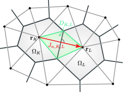
Figure 3: Delaunay triangulation and construction of Voronoï cells. The red arrow indicates the discrete current $J_{n,K,L}$ between two neighboring control volumes $\Omega_{K}$ and $\Omega_{L}$. The green area is the bi-hyperpyramid (or “diamond cell”) $D_{K,L}$ with height $\left\|\mathbf{r}_{L}-\mathbf{r}_{K}\right\|$ and internal face $|\partial\Omega_{L}\cap\partial\Omega_{K}|$. Adapted, with permission, from Ref. [89]. © 2019 IEEE.

3.2 Discretization of the current density expression

The discretization of $J_{n/p,K,L}$ is obtained by integrating the current density expressions (22) along the edge $\overline{KL}$ between two adjacent nodes of the mesh. Since the Kelvin formula implies a remarkably simple form of the electrical current densities in drift-diffusion form, where the thermal driving force is eliminated exactly (see Sec. 2.4), this allows for a straightforward adaptation of the Scharfetter–Gummel schemes developed for the isothermal case. We assume the electrostatic field $\mathbf{E}=-\nabla\phi$ and the temperature gradient $\nabla T$ to be constant along the edge $\overline{KL}$, such that

$$\phi\left(x\right) =x\,\phi_{L}+\left(1-x\right)\phi_{K}, T\left(x\right) =x\,T_{L}+\left(1-x\right)T_{K},$$

where $x\in\left[0,1\right]$ parametrizes the coordinate on the edge $\mathbf{r}\left(x\right)=x\thinspace\mathbf{r}_{L}+\left(1-x\right)\mathbf{r}_{K}$. Tacitly, these assumptions have already been used above in Eqs. (24a) and (24d). Moreover, also the mobilities $M_{n/p}$ and the fluxes $J_{n/p,K,L}$ are assumed to be constant on the edge. For the electron current density, this yields the two-point boundary value problem (BVP)

$$k_{B}T\left(x\right)g\left(\frac{n\left(x\right)}{N_{c}\left(T\left(x\right)\right)}\right)\frac{\mathrm{d}n}{\mathrm{d}x} =q\left(\phi_{L}-\phi_{K}\right)n\left(x\right)+\frac{J_{n,K,L}}{M_{n}}, n\left(0\right) =n_{K}, n\left(1\right) =n_{L},$$ (28)

on $x=\left[0,1\right]$. The problem for the holes current density is analogous.

In the non-degenerate case (Maxwell–Boltzmann statistics) the degeneracy factor is exactly $g\equiv 1$, such that the problem can be solved exactly by separation of variables. One obtains

$$\int_{n_{K}}^{n_{L}}\frac{\mathrm{d}n}{\frac{J_{n,K,L}}{qM_{n}\left(\phi_{L}-\phi_{K}\right)}+n} =\frac{q\left(\phi_{L}-\phi_{K}\right)}{k_{B}}\int_{0}^{1}\frac{\mathrm{d}x}{T\left(x\right)},$$

where the integral on the right hand side yields the (inverse) logarithmic mean temperature

$$\int_{0}^{1}\frac{\mathrm{d}x}{T\left(x\right)} =\int_{0}^{1}\frac{\mathrm{d}x}{x\,T_{L}+\left(1-x\right)T_{K}}=\frac{1}{\Lambda\left(T_{L},T_{K}\right)}\equiv\frac{1}{T_{K,L}}, \Lambda\left(x,y\right) =\frac{x-y}{\log{\left(x/y\right)}},$$ (29)

where $\Lambda\left(x,y\right)$ is the logarithmic mean. Solving for the flux yields the non-isothermal Scharfetter–Gummel scheme

$$J_{n,K,L}^{\text{ndeg}} =M_{n}k_{B}T_{K,L}\left(n_{L}B\left(X_{n,K,L}^{\text{ndeg}}\right)-n_{K}B\left(-X_{n,K,L}^{\text{ndeg}}\right)\right),\qquad X_{n,K,L}^{\text{ndeg}}=\frac{q\left(\phi_{L}-\phi_{K}\right)}{k_{B}T_{K,L}},$$ (30)

where $B\left(x\right)=x/\left(\exp{\left(x\right)}-1\right)$ is the Bernoulli function. The Bernoulli function is closely related to the logarithmic mean: $B\left(x\right)=1/\Lambda\left(\exp{(x)},1\right)$. At isothermal conditions $T_{K}\equiv T_{L}$, Eq. (30) reduces to the original Scharfetter–Gummel scheme [43].

In the case of Fermi–Dirac statistics ($g\neq 1$), no closed-form solution exists such that approximate solutions of the BVP (28) are required. As the degeneracy factor $g$ depends on both the carrier density and temperature, the problem is not even separable

3.2.1 Modified thermal voltage scheme

Following Refs. [54, 56], we solve the BVP (28) by freezing the degeneracy factor $g\left(n/N_{c}\left(T\right)\right)\to g_{n,K,L}$ to a carefully chosen average. The resulting problem has the same structure as in the non-degenerate case (see above), but with a modified thermal voltage $k_{B}T_{K,L}/q\to k_{B}T_{K,L}g_{n,K,L}/q$ along the edge, which takes the temperature variation and the degeneration of the electron gas into account. This yields the modified thermal voltage scheme

$$J_{n,K,L}^{g} =M_{n}k_{B}T_{K,L}g_{n,K,L}\left(n_{L}B\left(X_{n,K,L}^{g}\right)-n_{K}B\left(-X_{n,K,L}^{g}\right)\right),\qquad X_{n,K,L}^{g}=\frac{q\left(\phi_{L}-\phi_{K}\right)}{k_{B}T_{K,L}g_{n,K,L}},$$ (31a)

where $$T_{K,L} g_{n,K}\leq g_{n,K,L}\leq g_{n,L} \eta_{n,K}\leq\eta_{n,L} K\leftrightarrow L$$ is the logarithmic mean temperature (29). In order to ensure the consistency with the thermodynamic equilibrium and boundedness (for or with else), the edge-averaged degeneracy factor is taken as [54, 56]

$$g_{n,K,L}=\frac{\eta_{n,L}-\eta_{n,K}}{\log{\left(\mathscr{F}\left(\eta_{n,L}\right)/\mathscr{F}\left(\eta_{n,K}\right)\right)}}=\frac{\mathscr{F}^{-1}\left(n_{L}/N_{c}\left(T_{L}\right)\right)-\mathscr{F}^{-1}\left(n_{K}/N_{c}\left(T_{K}\right)\right)}{\log{\left(n_{L}/N_{c}\left(T_{L}\right)\right)}-\log{\left(n_{K}/N_{c}\left(T_{K}\right)\right)}}.$$ (31b)

In the limit of $\eta_{n,L}=\eta_{n,K}$, it approaches the common nodal value

$$\lim_{\eta_{n,L}\to\eta_{n,K}\equiv\bar{\eta}_{n}}g_{n,K,L}=\frac{\mathscr{F}\left(\bar{\eta}_{n}\right)}{\mathscr{F}^{\prime}\left(\bar{\eta}_{n}\right)}=g\left(\mathscr{F}\left(\bar{\eta}_{n}\right)\right)\equiv g_{\eta}\left(\bar{\eta}_{n}\right).$$

For constant temperature $T_{L}=T_{K}=T$, the scheme reduces to the modified Scharfetter–Gummel scheme discussed in Refs. [54, 56]. It can thus be regarded as a non-isothermal generalization of this approach. In the non-degenerate limit $g=1$, it reduces to the non-isothermal, non-degenerate Scharfetter–Gummel scheme (30).

3.2.2 Modified drift scheme

The traditional approach for the inclusion of degeneration effects in the Scharfetter–Gummel scheme, that is widely used in commercial software packages, is based on introducing the correction factors [52, 90, 91]

$$\gamma\left(\eta\right)=\frac{\mathscr{F}\left(\eta\right)}{\exp\left(\eta\right)},$$ (32)

and rearranging the current density expression with nonlinear diffusion (22) (involving the generalized Einstein relation (23)) into a form with linear diffusion and a modified drift term:

$$\mathbf{j}_{n} =\sigma_{n}\mathbf{E}_{n}+M_{n}k_{B}T\nabla n+\frac{k_{B}}{q}\sigma_{n}\thinspace\rho_{n}\left(T,\eta_{n}\right)\nabla T, \mathbf{E}_{n} =-\nabla\left(\phi+\frac{k_{B}T}{q}\log\left(\gamma\left(\eta_{n}\right)\right)\right).$$ (33)

Here, the degeneration of the electron gas induces a thermodiffusion term with the coefficient

$$\rho_{n}\left(T,\eta_{n}\right)=\log\left(\gamma\left(\eta_{n}\right)\right)-\frac{TN_{c}^{\prime}\left(T\right)}{N_{c}\left(T\right)}\frac{\gamma^{\prime}\left(\eta_{n}\right)/\gamma\left(\eta_{n}\right)}{1+\gamma^{\prime}\left(\eta_{n}\right)/\gamma\left(\eta_{n}\right)}=\log\left(\gamma\left(\eta_{n}\right)\right)+\frac{TN_{c}^{\prime}\left(T\right)}{N_{c}\left(T\right)}\left(g_{\eta}\left(\eta_{n}\right)-1\right),$$ (34)

that vanishes exactly in the non-degenerate limit ${\gamma\left(\eta\right)\equiv 1\equiv g_{\eta}\left(\eta\right)}$. Hence, the function $\rho_{n}\left(T,\eta_{n}\right)$ quantifies the difference between the degenerate and the non-degenerate Seebeck-coefficient, see Fig. 2 (a). On the step from Eq. (22) to (33), we have used the relation $g_{\eta}\left(\eta\right)=\left(1+\gamma^{\prime}\left(\eta\right)/\gamma\left(\eta\right)\right)^{-1}$. A plot of the correction factor (32) is given in Fig. 1 (c).

The current density expression (33) is discretized by projecting the current on the edge $\overline{KL}$, assuming the effective electric field $\mathbf{E}_{n}$ to be a constant along the edge, and freezing $\rho_{n}\left(T,\eta_{n}\right)\to\rho_{n,K,L}$ to a constant average value. Here, different averages can be taken for $\rho_{n,K,L}$, see Fig. 4 (c). The influence of this choice will be discussed below in Sec. 3.4. Along the same lines as above, one arrives at the modified drift scheme

$$\begin{aligned} J_{n,K,L}^{\gamma}\end{aligned} =M_{n}k_{B}T_{K,L}\left(n_{L}B\left(X_{n,K,L}^{\gamma}\right)-n_{K}B\left(-X_{n,K,L}^{\gamma}\right)\right),$$ (35a)

with

$$X_{n,K,L}^{\gamma}=\frac{q\left(\phi_{L}-\phi_{K}\right)}{k_{B}T_{K,L}}+\frac{T_{L}\log\left(\gamma\left(\eta_{n,L}\right)\right)-T_{K}\log\left(\gamma\left(\eta_{n,K}\right)\right)}{T_{K,L}}-\rho_{n,K,L}\log{\left(\frac{T_{L}}{T_{K}}\right)}.$$ (35b)

Again, $T_{K,L}$ is the logarithmic mean temperature (29). The corresponding non-degenerate limit (30) is easily recovered by $\gamma\left(\eta_{n,L/K}\right)\to 1$ and $\rho_{n,K,L}\to 0$.

3.3 Limiting cases and structure preserving properties

In the following, we investigate some important limiting cases and structure preserving properties of the generalized Scharfetter–Gummel schemes (31) and (35). This includes an analysis of the consistency of the discrete expressions with fundamental thermodynamical principles (thermodynamic equilibrium, second law of thermodynamics). To this end, it is convenient to rewrite both expressions using the identity $B\left(-x\right)=\exp{\left(x\right)}\,B\left(x\right)$ and the logarithmic mean $\Lambda$ (see Eq. (29)) as

$$J_{n,K,L}^{g} =-\sigma_{n,K,L}^{g}\left(\varphi_{n,L}-\varphi_{n,K}+P_{n,K,L}^{g}\left(T_{L}-T_{K}\right)\right) \text{with}\quad\sigma_{n,K,L}^{g}= qM_{n}\frac{\Lambda\left(n_{L}\exp{\left(-\frac{1}{2}X_{n,K,L}^{g}\right)},n_{K}\exp{\left(\frac{1}{2}X_{n,K,L}^{g}\right)}\right)}{\mathrm{sinhc}{\left(\frac{1}{2}X_{n,K,L}^{g}\right)}},$$ (36)

and

$$J_{n,K,L}^{\gamma} =-\sigma_{n,K,L}^{\gamma}\left(\varphi_{n,L}-\varphi_{n,K}+P_{n,K,L}^{\gamma}\left(T_{L}-T_{K}\right)\right) \text{with}\quad\sigma_{n,K,L}^{\gamma}= qM_{n}\frac{\Lambda\left(n_{L}\exp{\left(-\frac{1}{2}X_{n,K,L}^{\gamma}\right)},n_{K}\exp{\left(\frac{1}{2}X_{n,K,L}^{\gamma}\right)}\right)}{\mathrm{sinhc}{\left(\frac{1}{2}X_{n,K,L}^{\gamma}\right)}},$$ (37)

where $\mathrm{sinhc}\left(x\right)=\sinh{\left(x\right)}/x$. This representation directly corresponds to the continuous current density expression in the thermodynamic form (8), where the conductivity along the edge $\sigma_{n,K,L}^{g/\gamma}$ is determined by a “tilted” logarithmic average of the nodal carrier densities. Both expressions (36)–(37) have a common structure, but differ in the discrete conductivity $\sigma_{n,K,L}^{g}\neq\sigma_{n,K,L}^{\gamma}$ (due to $X_{n,K,L}^{g}\neq X_{n,K,L}^{\gamma}$) and the discrete Seebeck coefficients $P_{n,K,L}^{g}\neq P_{n,K,L}^{\gamma}$ along the edge, which are implicitly prescribed by the Scharfetter–Gummel discretization procedure. The latter read

$$P_{n,K,L}^{g} =-\frac{k_{B}}{q}\left[\log{\left(\frac{N_{c}\left(T_{L}\right)}{N_{c}\left(T_{K}\right)}\right)}\frac{g_{n,K,L}}{\log{\left(T_{L}/T_{K}\right)}}-\frac{\left(T_{L}-T_{K,L}\right)\eta_{n,L}-\left(T_{K}-T_{K,L}\right)\eta_{n,K}}{T_{L}-T_{K}}-\frac{1}{k_{B}}\frac{E_{c}\left(T_{L}\right)-E_{c}\left(T_{K}\right)}{T_{L}-T_{K}}\right]$$ (38a)

and

$$P_{n,K,L}^{\gamma} =-\frac{k_{B}}{q}\Bigg{[}\log{\left(\frac{N_{c}\left(T_{L}\right)}{N_{c}\left(T_{K}\right)}\right)}\frac{1}{\log{\left(T_{L}/T_{K}\right)}}+\rho_{n,K,L}-\frac{T_{L}\log\left(\gamma\left(\eta_{n,L}\right)\right)-T_{K}\log\left(\gamma\left(\eta_{n,K}\right)\right)-T_{K,L}\log{\left(\gamma\left(\eta_{n,L}\right)/\gamma\left(\eta_{n,K}\right)\right)}}{T_{L}-T_{K}}$$ (38b)

$$\phantom{=-\frac{k_{B}}{q}\Bigg{[}\log{\left(\frac{N_{c}\left(T_{L}\right)}{N_{c}\left(T_{K}\right)}\right)}\frac{1}{\log{\left(T_{L}/T_{K}\right)}}+\rho_{n,K,L}}-\frac{\left(T_{L}-T_{K,L}\right)\eta_{n,L}-\left(T_{K}-T_{K,L}\right)\eta_{n,K}}{T_{L}-T_{K}}-\frac{1}{k_{B}}\frac{E_{c}\left(T_{L}\right)-E_{c}\left(T_{K}\right)}{T_{L}-T_{K}}\Bigg{]}.$$

The discrete Seebeck coefficients (38) enter the discrete Joule heat term (27a) and thus the discrete entropy production rate (see Sec. 3.3.5 below). Out of the thermodynamic equilibrium, the discrete Seebeck coefficients (38) determine the point of compensating (discrete) chemical and thermal current flow such that $J_{n,K,L}|_{\varphi_{n,K}\neq\varphi_{n,L},T_{K}\neq T_{L}}=0$. In other words, there is a non-equilibrium configuration with $T_{K}\neq T_{L}$ and $\varphi_{n,K}\neq\varphi_{n,L}$, where the discrete Seebeck coefficient $P_{n,K,L}^{g/\gamma}=-\left(\varphi_{n,L}-\varphi_{n,K}\right)/\left(T_{L}-T_{K}\right)$ equals the (negative) ratio of both discrete driving forces such that the discrete current density is zero. This compensation point is in general slightly different between both schemes (see inset of Fig. 4 (c)). In the limit of a small temperature gradient and a small difference in the reduced Fermi energy along the edge, both discrete Seebeck coefficients approach in leading order the continuous expression (16a)

$$P_{n,K,L}^{g/\gamma}=-\frac{k_{B}}{q}\left[\frac{\bar{T}N_{c}^{\prime}(\bar{T})}{N_{c}(\bar{T})}g_{\eta}\left(\bar{\eta}_{n}\right)-\bar{\eta}_{n}-\frac{1}{k_{B}}E_{c}^{\prime}(\bar{T})\right]+\mathcal{O}(\delta\eta_{n}^{2})+\mathcal{O}(\delta\eta_{n}\,\delta\Theta)+\mathcal{O}(\delta\Theta^{2}),$$

where $\delta\Theta=\left(T_{L}-T_{K}\right)/\bar{T}$, $\bar{T}=\frac{1}{2}\left(T_{L}+T_{K}\right)$, $\delta\eta_{n}=\eta_{n,L}-\eta_{n,K}$ and $\bar{\eta}_{n}=\frac{1}{2}\left(\eta_{n,L}+\eta_{n,K}\right)$.

3.3.1 Thermodynamic equilibrium

In the thermodynamic equilibrium (thermal equilibrium $T_{K}=T_{L}$ and chemical equilibrium $\varphi_{n,K}=\varphi_{n,L}$), both the discrete current densities (31) and (35) are exactly zero. This is easily seen from Eqs. (36)–(37), where the discrete driving force $\left(\varphi_{n,L}-\varphi_{n,K}+P_{n,K,L}^{g/\gamma}\left(T_{L}-T_{K}\right)\right)$ vanishes under thermodynamic equilibrium conditions.

3.3.2 Strong electric field (drift-dominated limit)

Due to the asymptotics of the Bernoulli function $B\left(x\to\infty\right)=0$ and $B\left(x\to-\infty\right)\sim-x$, the modified thermal voltage scheme (31) approaches the first-order upwind scheme

$$J_{n,K,L}^{g}\left(\delta\phi_{K,L}\to\pm\infty\right) \sim-qM_{n}\left(\frac{n_{L}+n_{K}}{2}+\frac{n_{K}-n_{L}}{2}\mathop{\mathrm{sign}}\left(\delta\phi_{K,L}\right)\right)\,\delta\phi_{K,L}=J_{n,K,L}^{\text{{upw}}}$$ (39)

in the limit of a strong electrostatic potential gradient $\delta\phi_{K,L}=\phi_{L}-\phi_{K}\to\pm\infty$. The upwind scheme is a stable, first-order accurate discretization for advection-dominated problems, where the coefficient is evaluated in the “donor cell” of the flow [92]. Hence, this asymptotic feature of the original Scharfetter–Gummel scheme, which is important for the robustness of the discretization as it avoid spurious oscillations, is preserved in the degenerate and non-isothermal case. The modified drift scheme (35) approaches the upwind scheme as well

$$J_{n,K,L}^{\gamma}\left(\delta\phi_{K,L}\to\pm\infty\right) \sim-qM_{n}\left(\frac{n_{L}+n_{K}}{2}+\frac{n_{K}-n_{L}}{2}\mathop{\mathrm{sign}}\left(\delta\phi_{K,L}\right)\right)\left(\delta\phi_{K,L}+\frac{k_{B}}{q}\left(\log\left(\frac{\left[\gamma\left(\eta_{n,L}\right)\right]^{T_{L}}}{\left[\gamma\left(\eta_{n,K}\right)\right]^{T_{K}}}\right)-\left(T_{L}-T_{K}\right)\rho_{n,K,L}\right)\right),$$

however, in the case of strong degeneration the convergence is significantly slowed down if the nodal correction factors $\gamma\left(\eta_{n,K}\right)\neq\gamma\left(\eta_{n,K}\right)$ and temperatures $T_{L}\neq T_{K}$ are very different. This is shown in Fig. 4 (c), where the modified drift scheme shows a constant offset from the numerically exact solution of the BVP (28) for $\delta\phi_{K,L}\to-\infty$.

3.3.3 No electric field (diffusive limit)

In the case of a vanishing electrostatic potential gradient $\delta\phi_{K,L}=\phi_{L}-\phi_{K}=0$ the schemes take the form

$$\lim_{\delta\phi_{K,L}\to 0}J_{n,K,L}^{g} =M_{n}k_{B}T_{K,L}g_{n,K,L}\left(n_{L}-n_{K}\right),$$ (40)

$$\lim_{\delta\phi_{K,L}\to 0}J_{n,K,L}^{\gamma} =M_{n}k_{B}T_{K,L}\frac{1}{\Lambda\left(\frac{T_{L}^{\rho_{n,K,L}}}{\left[\gamma\left(\eta_{n,L}\right)\right]^{T_{L}/T_{K,L}}},\frac{T_{K}^{\rho_{n,K,L}}}{\left[\gamma\left(\eta_{n,K}\right)\right]^{T_{K}/T_{K,L}}}\right)}\left(\frac{T_{L}^{\rho_{n,K,L}}}{\left[\gamma\left(\eta_{n,L}\right)\right]^{T_{L}/T_{K,L}}}n_{L}-\frac{T_{K}^{\rho_{n,K,L}}}{\left[\gamma\left(\eta_{n,K}\right)\right]^{T_{K}/T_{K,L}}}n_{K}\right).$$

The modified thermal voltage scheme (31) approaches the central finite difference discretization (40), which is a stable discretization for diffusion-dominated transport problems [92]. With the edge-averaged degeneracy factor $g_{n,K,L}$, Eq. (40) nicely reflects the structure of the diffusive part of the continuous current density expression (22) involving the generalized Einstein relation (23). For the modified drift scheme (35), the limiting expression is a weighted finite difference discretization. Due to the different treatment of the degeneracy of the electron gas via the correction factors (32), it does not yield a discrete analogue of the generalized Einstein relation.

3.3.4 Purely thermally driven currents

In the chemical equilibrium ($\varphi_{n,L}=\varphi_{n,K}$), the current is driven only by the temperature gradient. The corresponding expressions are easily obtained from Eqs. (36)–(37), which include the discrete Seebeck coefficients (38).

3.3.5 Non-negativity of the discrete dissipation rate

The continuous entropy production rate (dissipation rate) per volume (see Eq. (53))

$$\dot{s}_{\text{tot}} =\frac{1}{T}\left(\mu_{c}-\mu_{v}\right)R+\frac{\kappa}{T^{2}}\left\|\nabla T\right\|^{2}+\frac{1}{T}H_{J},$$

has contributions from carrier recombination, heat flux and Joule heating $H_{J}=-\left(\nabla\varphi_{n}+P_{n}\nabla T\right)\cdot\mathbf{j}_{n}-\left(\nabla\varphi_{p}+P_{p}\nabla T\right)\cdot\mathbf{j}_{p}$. With the current density expressions (8) and a recombination rate of the form (9), all terms in $\dot{s}_{\text{tot}}$ (including $H_{J}$) are evidently non-negative (i. e., zero in the thermodynamic equilibrium and positive else). Therefore, the model obeys the second law of thermodynamics. In order to rule out unphysical phenomena such as steady state dissipation [54, 93], it is highly desirable to preserve this important structural property of the continuous system in its discrete counterpart. Given the finite volume discretization described above, this is straightforwardly achieved for the contributions from the carrier recombination and the heat flux, however, it is less obvious for the Joule heating term. In fact, the non-negativity of the discrete Joule heating term is non-trivial and can be violated in general when using a naive discretization approach as in Ref. [94].

We show that the discrete dissipation rate is evidently non-negative for both generalized Scharfetter–Gummel schemes (31) and (35). This follows immediately from their consistency with the thermodynamic equilibrium (see Sec. 3.3.1) in conjunction with the discrete form (27a) of the heating term. Substituting Eq. (36) in (27a), one obtains

$$H_{J,n}^{g} =-\left(\varphi_{n,L}-\varphi_{n,K}+P_{n,K,L}^{g}\left(T_{L}-T_{K}\right)\right)J_{n,K,L}^{g}=\sigma_{n,K,L}^{g}\left|\varphi_{n,L}-\varphi_{n,K}+P_{n,K,L}^{g}\left(T_{L}-T_{K}\right)\right|^{2}\geq 0,$$

which is zero only in the (discrete) thermodynamic equilibrium and positive else. The discrete conductivity $\sigma_{n,K,L}^{g}$ is positive by construction, see Eq. (36). Analogous expressions are obtained for the holes’ current contribution and the modified drift scheme (35). In conclusion, the consistency of the discrete system (24) with the second law of thermodynamics relies on using the respective Seebeck coefficients $P_{n/p,K,L}$ implied by the current discretization (see Eq. (38)) consistently in the discretized Joule heating term (27a). Only then this structural property of the discrete system holds without any smallness assumption.

3.4 Comparison with numerically exact solution

We investigate the accuracy of the schemes (31) and (35) by comparing them with the numerically exact solution of the BVP (28). In the isothermal case, this has been carried out before in a similar way by Farrell et al. [95] (for different Scharfetter–Gummel schemes), which inspired the investigation of highly accurate Scharfetter–Gummel type discretizations based on the direct numerical integration of the arising integral equation using quadrature rules in Ref. [96]. In the present non-isothermal case, the problem is more complicated because of the spatially varying temperature distribution along the edge. It is convenient to recast the problem (28) into the form

$$\begin{aligned} \frac{\mathrm{d}y\left(x\right)}{\mathrm{d}x}&=\frac{\bar{T}}{T\left(x\right)}\left(\delta\Phi+\frac{N_{c}(\bar{T})}{N_{c}(T(x))}\frac{J}{\mathscr{F}\left(y\right)}-\delta\Theta\frac{T(x)N_{c}^{\prime}(T(x))}{N_{c}(T(x))}\frac{\mathscr{F}\left(y\right)}{\mathscr{F}^{\prime}\left(y\right)}\right),\\ y\left(0\right)&=\bar{\eta}_{n}-\frac{1}{2}\delta\eta_{n},\qquad\qquad y\left(1\right)=\bar{\eta}_{n}+\frac{1}{2}\delta\eta_{n},\end{aligned}$$ (41)

with the notations $T\left(x\right)\equiv\left(1+\left[x-\frac{1}{2}\right]\delta\Theta\right)\bar{T}$, $\bar{T}=\frac{1}{2}\left(T_{L}+T_{K}\right)$, $\delta T=T_{L}-T_{K}$, $\bar{\eta}_{n}=\frac{1}{2}\left(\eta_{n,L}+\eta_{n,K}\right)$, $\delta\eta_{n}=\eta_{n,L}-\eta_{n,K}$ and the non-dimensionalized quantities

$$J =\frac{J_{n,K,L}}{M_{n}k_{B}\bar{T}N_{c}(\bar{T})}, \delta\Phi =\frac{q\left(\phi_{L}-\phi_{K}\right)}{k_{B}\bar{T}}, \delta\Theta =\frac{\delta T}{\bar{T}}.$$

The exact current $J_{\text{exact}}=J_{\text{exact}}(\delta\Phi,\delta\eta_{n},\delta\Theta,\bar{\eta}_{n},\bar{T})$ is a function of five parameters that satisfies the BVP (41). We solve the BVP (41) numerically using the shooting method [97], where we combine a 4th order Runge–Kutta method with Brent’s root finding algorithm [98] . The problem is invariant under the simultaneous transformation

$$\delta\Phi \to-\delta\Phi, \delta\eta_{n} \to-\delta\eta_{n}, \delta\Theta \to-\delta\Theta, x \to 1-x, J \to-J$$

(i. e., the sign of the current changes when changing the nodes $K\leftrightarrow L$), such that we can restrict our analysis to $\delta\Theta\geq 0$, when exploring the accuracy of the discrete current in the $\left(\delta\Phi,\delta\eta_{n}\right)$-plane. The comparison is carried out for $\mathscr{F}\left(\eta\right)=F_{1/2}\left(\eta\right)$ and $N_{c}=2\left(m_{c}^{\ast}k_{B}T/(2\pi\hbar^{2})\right)^{3/2}$. The Fermi–Dirac integrals $F_{1/2}\left(\eta\right)$ and $F_{-1/2}\left(\eta\right)$ are evaluated using MacLeod’s algorithm [99].

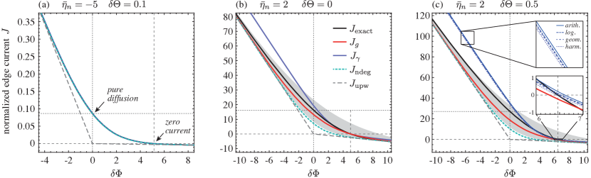
Figure 4: Comparison of the non-isothermal Scharfetter–Gummel schemes for $\delta\eta_{n}=5$. (a) In the non-degenerate regime ($\bar{\eta}_{n}=-5$) all schemes coincide, even in the presence of a temperature gradient. (b) At $\bar{\eta}_{n}=2$ degeneration effects become significant. While $J_{g}$ follows $J_{\text{exact }}$ with an acceptable error over the whole range of $\delta\Phi$, the modified drift scheme $J_{\gamma}$ has a significant offset at strong electric fields ($\delta\Phi\to-\infty$). The grey shaded area indicates the analytic bounds of the modified thermal voltage scheme determined using the nodal values $g_{n,K}$ and $g_{n,L}$ instead of $g_{n,K,L}$. (c) An additional temperature gradient increases the error in the degenerate regime. The insets show the effect of different averages $\rho_{n,K,L}$ of the nodal values $\rho_{n,K}$ and $\rho_{n,L}$ in the modified drift scheme and the different behavior of the schemes in the region of vanishing discrete currents.

Figure 4 shows the numerically exact current $J_{\text{exact}}$ along with the approximations $J_{g}$ (modified thermal voltage scheme (31)) and $J_{\gamma}$ (modified drift scheme (35)) as a function of the normalized electric field $\delta\Phi$ along the edge. For weak degeneracy, both schemes agree with the numerically exact solution – even in the case of non-isothermal conditions. This is shown in Fig. 4 (a) for $\bar{\eta}_{n}=-5$ and $\delta\Theta=0.1$. At strong electric fields $\delta\Phi\to\pm\infty$, all schemes approach the upwind scheme $J_{\text{upw}}$ (grey dashed line, cf. Eq. (39)). The schemes (31) and (35) differ in the treatment of degeneration effects, which becomes apparent for increased $\bar{\eta}_{n}$. Figure 4 (b) shows the results for $\bar{\eta}_{n}=2$ at isothermal conditions $\delta\Theta=0$. The modified thermal voltage scheme $J_{g}$ (red line) yields an acceptable deviation from the exact result $J_{\text{exact}}$ (black line) over the whole range of $\delta\Phi$. The error vanishes at strong electric fields where both $J_{g}$ and $J_{\text{exact}}$ converge to the upwind scheme $J_{\text{upw}}$. The modified drift scheme (purple line), however, shows a significant error at large (negative) $\delta\Phi$, where it overestimates the current density significantly (about 33 % relative error at $\delta\Phi=-3$). This behavior results from the different treatment of the degeneration effects, that degrades the convergence of the modified drift scheme in the case of strong degeneration (see Sec. 3.3.2). The plot highlights two other important exceptional points (pure diffusion and zero current), where both schemes show a similar accuracy. In the presence of an additional temperature gradient along the edge, see Fig. 4 (c), the approximation error of both schemes increases. The upper inset shows that the choice of the average of $\rho_{n,K,L}$ (see Eq. (34)) has only a minor impact on the modified drift scheme. The lower inset zooms on the region where the currents become zero. Here, all schemes provide a satisfying accuracy, but none of them is exact, i. e., they yield a small spurious discrete current and intersect with the exact solution only in the vicinity of the exact zero current point. We observe that the modified drift schemes show a slightly better performance in this case, i. e., the Seebeck coefficient (38b) appears to be slightly better than (38a).

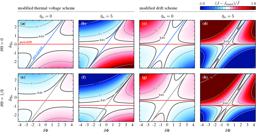
Figure 5: Comparison of the two non-isothermal Scharfetter–Gummel schemes (31) and (35) (with arithmetic average $\rho_{n,K,L}=\left(\rho_{n,K}+\rho_{n,L}\right)/2$) in the ($\delta\Phi,\delta\eta_{n}$)-plane at isothermal ($\delta\Theta=0$, top row (a)–(d)) and non-isothermal ($\delta\Theta=1/6$, bottom row (e)–(h)) conditions and different levels of degeneration (weak $\bar{\eta}_{n}=0$ or strong $\bar{\eta}_{n}=5$). The normalized absolute error $(J-J_{\text{exact}})/\hat{J}$ is color-coded for the range $[-1,1]$ (dark colored regions correspond to larger errors, see the level lines). See the text for a discussion.

The normalized absolute errors $(J-J_{\text{exact}})/\hat{J}$ (with $\hat{J}=M_{n}k_{B}\bar{T}N_{c}(\bar{T})$) of the two schemes (31) and (35) are shown in the ($\delta\Phi,\delta\eta_{n}$)-plane in Fig. 5 under isothermal ($\delta\Theta=0$, top row (a)–(d)) and non-isothermal ($\delta\Theta=1/6$, bottom row (e)–(h)) conditions and for different levels of degeneration (weak $\bar{\eta}_{n}=0$ and strong $\bar{\eta}_{n}=5$). In the limit of very fine meshes $(\delta\Phi,\delta\eta_{n},\delta\Theta)\to(0,0,0)$, both schemes coincide and the deviation from the exact current approaches zero. One observes that the size of the white regions with a normalized absolute error below $0.01$ (in the following denoted as “low error domain”) are generally larger for the modified thermal voltage scheme than for the modified drift scheme. Thus, the modified thermal voltage scheme is expected to yield a higher accuracy on sufficiently fine meshes. This will be evidenced by the numerical simulation of a p-n-diode in Sec. 3.6. The plots in Fig. 5 feature two additional lines, that refer to special limiting cases where both schemes yield a very high accuracy. The case of a pure drift current (i. e., no diffusion $n_{L}=n_{K}$) is indicated by a red line; the zero current line (blue) refers to the curve in the ($\delta\Phi,\delta\eta_{n}$)-plane where the exact current vanishes ($J_{\text{exact}}=0$ in the BVP (41)). In the isothermal case ($\delta\Theta=0$), the latter corresponds to the thermodynamic equilibrium, in the non-isothermal case $(\delta\Theta\neq 0)$ it refers to the situation of compensating chemical and thermal driving forces. Both schemes are exact in the case of a pure drift current, i. e., they asymptotically approach the upwind scheme (39), which is important for the robustness of the discretization in order to avoid spurious oscillations. The modified thermal voltage scheme shows a high accuracy also for slight deviations from the pure drift line, even in the case of strong degeneration, see Fig. 5 (b, f). In contrast, the modified drift scheme yields significant errors (much higher than $0.01$) already for tiny deviations from the pure drift line in the strongly degenerate case, see Fig. 5 (d, h). This behavior has already been observed above in Fig. 4 (b, c) and was predicted analytically in Sec. 3.3.2. Note that in the non-isothermal case, the temperature gradient shifts the pure drift line from $\delta\eta_{n}^{\text{pure drift}}|_{\delta\Theta=0}=0$ (in Fig. 5 (a–d)) to $\delta\eta_{n}^{\text{pure drift}}\approx-\delta\Theta g_{\eta}(\bar{\eta}_{n})\bar{T}N_{c}^{\prime}(\bar{T})/N_{c}(\bar{T})$ (see Fig. 5 (e–h)). A prominent feature of the modified drift scheme is the additional intersection with the exact solution (see also Fig. 4 (c) at $\delta\Phi\approx 3.5$), which leads to additional “fingers” of the low error domain, see Fig. 5 (c, d, g, h), that are not associated with any special limiting case. The same feature has been observed for the so-called inverse activity scheme described in Ref. [95]. Finally, we study the consistency of the discretization schemes with the zero current line. In the isothermal case, both schemes are exact and therefore consistent with the thermodynamic equilibrium, see Fig. 5 (a–d). In the strongly degenerate case, however, the zero current line is only partially located within the low error domain, since the schemes intersect with the exact solution only in the vicinity of the zero current line and not exactly on it (see also the inset of Fig. 4 (c)). Nevertheless, the zero current lines of the discrete schemes, which are plotted as dashed orange lines in Fig. 5 (e–h), nicely overlap with the exact zero current line (blue). Thus, the spurious non-zero currents are very low and the little discrepancy in this limiting case is only of minor importance.

3.5 Analytical error estimate

We compare both schemes (31) and (35) by deriving an upper error bound. We follow the approach developed by Farrell et al. [95] and extend it to the non-isothermal case. Using the identities

$$B\left(x\right)-B\left(-x\right) =-x, B\left(x\right)+B\left(-x\right) =x\coth{\left(\frac{x}{2}\right)},$$

we obtain the series expansion of the discrete currents (31) and (35) at $\left(\delta\Phi,\delta\eta_{n},\delta\Theta\right)=\left(0,0,0\right)$ up to second order as

$$J_{g} =-\mathscr{F}\left(\bar{\eta}_{n}\right)\delta\Phi+\mathscr{F}\left(\bar{\eta}_{n}\right)\left(\delta\eta+\frac{\bar{T}N_{c}^{\prime}(\bar{T})}{N_{c}(\bar{T})}g_{\eta}\left(\bar{\eta}_{n}\right)\delta\Theta\right)\frac{\tilde{X}_{g}}{2}\coth{\left(\frac{\tilde{X}_{g}}{2}\right)}+\mathcal{O}(\delta^{3}),$$

$$J_{\gamma} =-\mathscr{F}\left(\bar{\eta}_{n}\right)\tilde{X}_{\gamma}+\mathscr{F}^{\prime}\left(\bar{\eta}_{n}\right)\left(\delta\eta+\frac{\bar{T}N_{c}^{\prime}(\bar{T})}{N_{c}(\bar{T})}g_{\eta}\left(\bar{\eta}_{n}\right)\delta\Theta\right)\frac{\tilde{X}_{\gamma}}{2}\coth{\left(\frac{\tilde{X}_{\gamma}}{2}\right)}+\mathcal{O}(\delta^{3}),$$

where

$$\tilde{X}_{g} =\frac{1}{g_{\eta}\left(\bar{\eta}_{n}\right)}\delta\Phi, \tilde{X}_{\gamma} =\delta\Phi-\frac{g_{\eta}\left(\bar{\eta}_{n}\right)-1}{g_{\eta}\left(\bar{\eta}_{n}\right)}\left(\delta\eta+\frac{\bar{T}N_{c}^{\prime}(\bar{T})}{N_{c}(\bar{T})}g_{\eta}\left(\bar{\eta}_{n}\right)\delta\Theta\right),$$

and $\mathcal{O}(\delta^{3})\equiv\mathcal{O}(\delta\eta_{n}^{3})+\mathcal{O}(\delta\eta_{n}^{2}\,\delta\Theta)+\mathcal{O}(\delta\Theta^{2}\,\delta\eta_{n})+\mathcal{O}(\delta\Theta^{3})+\mathcal{O}(\delta\Phi\,\delta\eta_{n}^{2})+\mathcal{O}(\delta\Phi\,\delta\eta_{n}\,\delta\Theta)+\mathcal{O}(\delta\Phi\,\delta\Theta^{2})$ denotes the third-order corrections. The second-order expansion of the modified drift scheme is independent of the kind of average used for $\rho_{n,K,L}\approx\rho_{n}(\bar{\eta}_{n},\bar{T})+\mathcal{O}(\delta\eta_{n}^{2})+\mathcal{O}(\delta\eta_{n}\,\delta\Theta)+\mathcal{O}(\delta\Theta^{2})$, as only its zeroth-order contribution (where all means coincide) is relevant here. Using the inequality [95]

$$1\leq x\coth{\left(x\right)}\leq 1+\left|x\right|,$$

we arrive at the error estimates for the modified thermal voltage scheme (neglecting third-order terms)

$$\left|J_{g}-J_{1}\right| \leq\frac{1}{2}\mathscr{F}^{\prime}\left(\bar{\eta}_{n}\right)\left(\left|\delta\Phi\,\delta\eta_{n}\right|+\frac{\bar{T}N_{c}^{\prime}(\bar{T})}{N_{c}(\bar{T})}g_{\eta}\left(\bar{\eta}_{n}\right)\left|\delta\Phi\,\delta\Theta\right|\right)$$ (42)

and the modified drift scheme

$$\left|J_{\gamma}-J_{1}\right| \leq\frac{1}{2}\mathscr{F}^{\prime}\left(\bar{\eta}_{n}\right)\left(\left|\delta\Phi\,\delta\eta_{n}\right|+\frac{\bar{T}N_{c}^{\prime}(\bar{T})}{N_{c}(\bar{T})}g_{\eta}\left(\bar{\eta}_{n}\right)\left|\delta\Phi\,\delta\Theta\right|+\frac{g_{\eta}\left(\bar{\eta}_{n}\right)-1}{g_{\eta}\left(\bar{\eta}_{n}\right)}\left|\delta\eta_{n}+\frac{\bar{T}N_{c}^{\prime}(\bar{T})}{N_{c}(\bar{T})}g_{\eta}\left(\bar{\eta}_{n}\right)\delta\Theta\right|^{2}\right),$$ (43)

where $J_{1}=\mathscr{F}\left(\bar{\eta}_{n}\right)\left(\delta\eta_{n}-\delta\Phi+\frac{\bar{T}N_{c}^{\prime}(\bar{T})}{N_{c}(\bar{T})}g_{\eta}\left(\bar{\eta}_{n}\right)\delta\Theta\right)$ is the first-order exact solution of the BVP (41). Both schemes converge to the exact result as their first-order terms agree with $J_{1}$. The first two terms of Eq. (43) coincide with Eq. (42). The error bound for the modified drift scheme has an additional second-order contribution that becomes significant in the case of strong degeneration $\bar{\eta}\gg 1$ where $(g_{\eta}\left(\bar{\eta}_{n}\right)-1)/g_{\eta}\left(\bar{\eta}_{n}\right)\to 1$. Therefore, the maximum error of the modified thermal voltage scheme is guaranteed to be smaller than that of the modified drift scheme in the case of degenerate carrier statistics. This analytical result is consistent with the numerical results shown in Figs. 4 and 5 and holds in both the isothermal and the non-isothermal case. For non-degenerate carrier statistics, both error estimates (42) and (43) coincide, since both schemes reduce to the non-degenerate scheme (30).

3.6 Numerical simulation of a p-n-diode

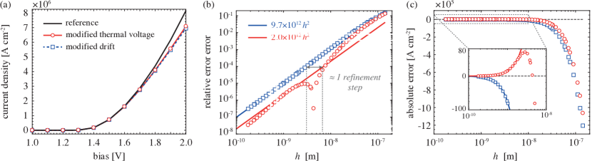
Figure 6: Convergence of total current density in the p-n diode problem without self-heating effects ($H=0$, isothermal case). (a) Current-voltage curves obtained by the two schemes (31) and (35) on an equidistant grid with 13 nodes. The reference solution (black line) was obtained on a fine grid (65535 nodes). (b) Convergence of the relative error with respect to the reference solution under mesh refinement at $2\,\text{V}$. The modified drift scheme (blue squares) shows a monotonous, quadratic convergence for decreasing $h$. The modified thermal voltage scheme (red circles) converges non-monotonously as it intersects with the reference solution at $h\approx 4.5\,\text{nm}$. (c) Convergence of the absolute error of both schemes.

We consider a one-dimensional GaAs-based p-n-diode and compare the convergence of the total current density ($\mathbf{j}_{\text{tot}}=\mathbf{j}_{n}+\mathbf{j}_{p}$) under mesh refinement using both discretization schemes. The device consists of a $1\,\text{\textmu m}$ n-doped section with $C=N_{D}^{+}=2\times 10^{18}\,\text{cm}^{-3}$ followed by a $1\,\text{\textmu m}$ long p-doped section with $C=-N_{A}^{-}=-2\times 10^{18}\,\text{cm}^{-3}$. We use Fermi–Dirac statistics $\mathscr{F}\left(\eta\right)=F_{1/2}\left(\eta\right)$ and take Shockley–Read–Hall recombination, spontaneous emission and Auger recombination into account [15, 62]. The material parameters, mobility models (depending on temperature and doping density) and the temperature-dependent heat conductivity model are taken from Ref. [62]. The mobilities and thermal conductivity along the edges are taken as the harmonic average of the respective nodal values. We use Dirichlet boundary conditions on both ends of the diode, modeling ideal Ohmic contacts (charge neutrality at the boundary) and ideal heat sinks with $T_{\text{contact}}=300\,\text{K}$. The simulations are carried out on equidistant grids with varying number of mesh points $N_{\text{nodes}}$ and mesh size $h=2\,\text{\textmu m}/(N_{\text{nodes}}-1)$. The nonlinear systems are solved using a Newton iteration method with a fully analytical Jacobian matrix [83].

Figure 6 (a) shows the current-voltage curves obtained by both discretization schemes on a coarse grid (13 nodes, $h\approx 1.7\times 10^{-7}\,\text{m}$) under isothermal conditions, i. e., without self-heating and Seebeck effect. For the evaluation of the error, we use a reference solution that was computed on a fine grid with 65535 nodes ($h\approx 3.1\times 10^{-11}\,\text{m}$), where the relative error between both schemes is about $9.6\times 10^{-9}$. At $2\thinspace\text{V}$ the computed currents differ significantly from the reference result: The relative error is about $13\,\%$ for the modified thermal voltage scheme and $15\,\%$ for the modified drift scheme. The convergence of the computed current densities to the reference result under mesh refinement is shown in Fig. 6 (b). The modified drift scheme (Eq. (35), blue squares) shows a monotonous, quadratic convergence for decreasing $h$. The modified thermal voltage scheme (Eq. (31), red circles), however, shows a non-monotonous convergence behavior as it intersects with the reference solution at $h\approx 4.5\times 10^{-9}\,\text{m}$. On sufficiently fine meshes ($h<10^{-8}\,\text{m}$), the error of the modified thermal voltage scheme is almost one order of magnitude smaller than that of the modified drift scheme. Conversely, the modified thermal voltage scheme reaches the same accuracy as the modified drift scheme already on a coarse grid with less than half of the number of nodes. Thus, the modified thermal voltage scheme saves about one refinement step. The convergence of the absolute error is plotted in Fig. 6 (c), where the inset highlights the origin of the non-monotonous convergence behavior of the modified thermal voltage scheme.

The numerical results for the non-isothermal case, where self-heating and the Seebeck effect are taken into account, are shown in Fig. 7. The results are qualitatively very similar to the isothermal case shown in Fig. 6; quantitatively the advantage of the modified thermal voltage scheme over the modified drift scheme is even greater. On a coarse grid, the total current is underestimated by both schemes with a relative error of about $8\,\%$, see Fig. 7 (a). For sufficiently fine meshes ($h<0.5\times 10^{-8}\text{m}$), the error of the modified thermal voltage scheme is always more than one order of magnitude smaller than that of the modified drift scheme, see Fig. 7 (b). In other words, the modified thermal voltage scheme reaches the same accuracy already on an about four times coarser mesh (two refinement steps), which is a substantial advantage for large problems involving complex multi-dimensional geometries. Again, we observe a non-monotonous convergence behavior of the modified thermal voltage scheme, see Fig. 7 (b, c).

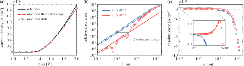
Figure 7: Convergence of total current density in the p-n diode problem with self-heating effects. (a) Current-voltage curves obtained by the two schemes (31) and (35) on an equidistant grid with 13 nodes. As in Fig. 6, the reference solution (black line) was obtained on a grid with 65535 nodes. Self-heating lowers the mobilities such that the total current density is smaller than in the isothermal case, cf. Fig. 6 (a). (b) Convergence of the relative error with respect to the reference solution under mesh refinement at $2\,\text{V}$. As in the isothermal case, the modified thermal voltage scheme (red circles) shows a non-monotonous convergence behavior that is faster than the quadratic convergence of the modified drift scheme (blue squares). (c) Convergence of the absolute error of both schemes. The modified thermal voltage scheme intersects twice with the reference solution.

4 Summary and conclusion

We discussed the non-isothermal drift-diffusion system for the simulation of electro-thermal transport processes in semiconductor devices. It was shown that the model equations take a remarkably simple form when assuming the Kelvin formula for the Seebeck coefficient. First, the heat generation rate involves exactly the three classically known self-heating effects (Joule heating, recombination heating, Thomson–Peltier effect) without any further transient contributions. Moreover, our modeling approach immediately yields the correct average kinetic energy of the carriers in the recombination heating term, independently of any scattering parameter. Second, the Kelvin formula enables a simple representation of the electrical current densities in the drift-diffusion form, where the thermal driving force can be entirely absorbed in the (nonlinear) diffusion coefficient via the generalized Einstein relation. The Kelvin formula accounts for the degeneration of the electron-hole plasma (Fermi–Dirac statistics) and was shown to be in a good quantitative agreement with experimental data reported for n-GaAs.

We have derived two non-isothermal generalizations of the finite volume Scharfetter–Gummel scheme for the discretization of the current densities, which differ in their treatment of degeneration effects. The first approach is based on an approximation of the discrete generalized Einstein relation and implies a specific modification of the thermal voltage. The second scheme is based on including the degeneration effects into a modification of the electric field, which is similar to the conventional method that is widely used in commercial device simulation software packages [90, 91]. We presented a detailed analysis of both schemes by assessing their accuracy in comparison to the numerically exact solution of the underlying two-point boundary value problem. Moreover, we derived analytical error bounds and investigated important structure preserving properties of the discretizations, including the consistency with the thermodynamic equilibrium, the non-negativity of the discrete dissipation rate (second law of thermodynamics on the discrete level) and their asymptotic behavior in the drift- and diffusion-dominated limits. Finally, we performed a numerical convergence study for a simple example case. Our results indicate a significantly higher accuracy and faster convergence of the modified thermal voltage scheme in comparison to the modified drift scheme. This result holds under both isothermal and non-isothermal conditions. The higher accuracy — about one order of magnitude for sufficiently fine grids in the present case study — of the modified thermal voltage scheme makes it a favorable discretization method for problems exhibiting stiff solutions (internal layers at p-n junctions, boundary layers at electrical contacts) or devices with a complicated multi-dimensional geometry, where the number of nodes required to reach the asymptotic accuracy regime is extremely large and routinely exceeds the available computational power.

In more general situations, where the Seebeck coefficient deviates from the Kelvin formula (e. g., due to the phonon drag effect), we suggest to combine the two discretization techniques by decomposing the Seebeck coefficient into a Kelvin formula part and an excess contribution: $P_{n}=P_{n}^{\text{Kelvin}}+P_{n}^{\text{exc}}$. The first part can be absorbed in the generalized Einstein relation, which allows for the treatment described in Sec. 3.2.1 and inherits the improved accuracy of the modified thermal voltage scheme. The excess part $P_{n}^{\text{exc}}$ must be averaged along the edge and plays a similar role as the $\rho_{n,K,L}$ term in Sec. 3.2.2 (leading to an additive correction in the argument of the Bernoulli function).

Appendix Appendix A Non-parabolic energy bands

The results presented in this paper hold for Fermi–Dirac statistics with arbitrary density of states, provided that the Kelvin formula for the Seebeck coefficient is applicable. In particular, this includes also the case of non-parabolic energy bands. For example, we assume the scalar Kane-type model [28] for the conduction band energy dispersion

$$E =E_{c}+\varepsilon_{k}, \left(1+\alpha\varepsilon_{k}\right)\varepsilon_{k} =\frac{\hbar^{2}k^{2}}{2m_{c}^{\ast}}$$

with the non-parabolicity parameter $\alpha\geq 0.$ This corresponds to the density of states (in 3D)

$$D_{c}\left(E\right)=\frac{1}{V}\sum_{\mathbf{k},\sigma}\delta\left(E-E\left(\mathbf{k}\right)\right)=\frac{1}{2\pi^{2}}\left(\frac{2m_{c}^{\ast}}{\hbar^{2}}\right)^{3/2}\sqrt{\left(E-E_{c}\right)\left(1+\alpha\left(E-E_{c}\right)\right)}\left(1+2\alpha\left(E-E_{c}\right)\right)\,\Theta\left(E-E_{c}\right),$$

which recovers with the parabolic case for $\alpha=0$. Here, $\Theta$ is the Heaviside step function. For weak non-parabolicity $0\leq\alpha/\beta\ll 1$, the corresponding electron density can be expanded in a series of Fermi–Dirac integrals (7)

$$n =\int_{\mathbb{R}}\mathrm{d}E\,D_{c}\left(E\right)\frac{1}{\exp{\left(\beta\left[E-q\phi-\mu_{c}\right]\right)}+1}=N_{c}\left(T\right)\mathscr{F}\left(\eta_{n}\right), \mathscr{F}\left(\eta_{n}\right) =\sum_{n=0}^{\infty}\frac{1}{n!}\frac{\Gamma\left(\frac{5}{2}+n\right)}{\Gamma\left(\frac{5}{2}-n\right)}\left(\frac{\alpha}{\beta}\right)^{n}F_{n+\frac{1}{2}}\left(\eta_{n}\right),$$

with $\eta_{n}=\beta\left(\mu_{c}+q\phi-E_{c}\right)$ and $\beta=\left(k_{B}T\right)^{-1}$, which is clearly of the type (5).

The desired asymptotic behavior in the non-degenerate limit $\mathscr{F}(\eta\ll-1)\sim\exp{(\eta)}$ is restored by rescaling

$$N_{c}\left(T\right) \to\sqrt{\frac{\beta}{\pi\alpha}}\exp{\left(\frac{\beta}{2\alpha}\right)}K_{2}\left(\frac{\beta}{2\alpha}\right)N_{c}\left(T\right), \mathscr{F}(\eta) \to\left(\sqrt{\frac{\beta}{\pi\alpha}}\exp{\left(\frac{\beta}{2\alpha}\right)}K_{2}\left(\frac{\beta}{2\alpha}\right)\right)^{-1}\mathscr{F}(\eta),$$

where $K_{\nu}$ is the modified Bessel function of second kind.

Appendix Appendix B Generalization to the case of multiple temperatures

The results for the Kelvin formula can be generalized to the multi-temperature case, i.e., to systems describing hot carrier transport where the carrier ensembles have temperatures different from the lattice temperature $T_{n}\neq T_{L}\neq T_{p}$. We postulate the free energy density of the electron-hole plasma

$$\begin{aligned} f_{\text{e--h}}\left(n,p,T_{n},T_{p},T_{L}\right)&=k_{B}T_{n}\left[n\mathscr{F}^{-1}\left(\frac{n}{N_{c}\left(T_{L},T_{n}\right)}\right)-N_{c}\left(T_{n},T_{L}\right)\mathscr{G}\left(\mathscr{F}^{-1}\left(\frac{n}{N_{c}\left(T_{n},T_{L}\right)}\right)\right)\right]+nE_{c}\left(T_{L}\right)\\ &\phantom{=}+k_{B}T_{p}\left[p\mathscr{F}^{-1}\left(\frac{p}{N_{v}\left(T_{p},T_{L}\right)}\right)-N_{v}\left(T_{p},T_{L}\right)\mathscr{G}\left(\mathscr{F}^{-1}\left(\frac{p}{N_{v}\left(T_{p},T_{L}\right)}\right)\right)\right]-pE_{v}\left(T_{L}\right),\end{aligned}$$ (44)

where the effective density of states $N_{c/v}=N_{c/v}(T_{n/p},T_{L})$ is now a function of the carrier temperature and the lattice temperature. In the case of 3D bulk materials, this might be for example $N_{c/v}=2\left(m_{e/h}^{\ast}\left(T_{L}\right)k_{B}T_{n/p}/(2\pi\hbar^{2})\right)^{3/2}$, where the effective masses are allowed to depend on the lattice temperature $T_{L}$. Moreover, the band gap energy and the band edge energies $E_{c/v}$ depend solely on $T_{L}$. The free energy density of the phonon gas $f_{L}=f_{L}\left(T_{L}\right)$ and the electrostatic interaction energy $f_{\text{Coul}}=f_{\text{Coul}}\left(p-n\right)$ are the same as in Sec. 2.1.

The multi-temperature free energy density $f\left(n,p,T_{n},T_{p},T_{L}\right)=f_{\text{e--h}}\left(n,p,T_{n},T_{p},T_{L}\right)+f_{\text{Coul}}\left(p-n\right)+f_{L}\left(T_{L}\right)$ is a thermodynamic potential, that yields expressions for the chemical potentials

$$+\mu_{c} =\frac{\partial f}{\partial n}=k_{B}T_{n}\mathscr{F}^{-1}\left(\frac{n}{N_{c}\left(T_{n},T_{L}\right)}\right)+E_{c}\left(T_{L}\right)-q\phi$$ (45a)

$$-\mu_{v} =\frac{\partial f}{\partial p}=k_{B}T_{p}\mathscr{F}^{-1}\left(\frac{p}{N_{v}\left(T_{p},T_{L}\right)}\right)-E_{v}\left(T_{L}\right)+q\phi$$ (45b)

and the entropy densities

$$s_{n} =-\frac{\partial f}{\partial T_{n}}, s_{p} =-\frac{\partial f}{\partial T_{p}}, s_{L} =-\frac{\partial f}{\partial T_{L}}.$$

The state equations for the carrier densities follow from Eq. (45) as

$$n =N_{c}\left(T_{n},T_{L}\right)\mathscr{F}\left(\frac{\mu_{c}+q\phi-E_{c}\left(T_{L}\right)}{k_{B}T_{n}}\right), p =N_{v}\left(T_{p},T_{L}\right)\mathscr{F}\left(\frac{E_{v}\left(T_{L}\right)-q\phi-\mu_{v}}{k_{B}T_{p}}\right).$$

In analogy to Eq. (8), we postulate the generalized electrical current density expressions

$$\mathbf{j}_{n} =-\sigma_{n}\left(\nabla\varphi_{n}+P_{n,n}\nabla T_{n}+P_{L,n}\nabla T_{L}\right), \mathbf{j}_{p} =-\sigma_{p}\left(\nabla\varphi_{p}+P_{p,p}\nabla T_{p}+P_{L,p}\nabla T_{L}\right),$$ (46)

with the thermopowers given by the Kelvin formula

$$P_{n,n} =-\frac{1}{q}\frac{\partial s_{n}}{\partial n}, P_{L,n} =-\frac{1}{q}\frac{\partial s_{L}}{\partial n}, P_{p,p} =+\frac{1}{q}\frac{\partial s_{p}}{\partial p}, P_{L,p} =+\frac{1}{q}\frac{\partial s_{L}}{\partial p}.$$ (47)

Here, we do not describe the corresponding hot carrier transport system in full detail, but rather focus on the central property of the electrical current densities, which is the simple representation in the drift-diffusion form (without thermodiffusion). If the thermal driving forces can be absorbed in a generalized Einstein relation for the diffusion coefficient, this enables a generalized Scharfetter–Gummel discretization of type (31) (modified thermal voltage scheme). With the definitions given above, the drift-diffusion form of Eq. (46) reads (along the lines in Sec. 2.4)

$$\mathbf{j}_{n} =-\sigma_{n}\left(-\frac{1}{q}\nabla\mu_{c}+P_{n,n}\nabla T_{n}+P_{L,n}\nabla T_{L}\right)=-\sigma_{n}\left(-\frac{1}{q}\nabla\frac{\partial f}{\partial n}+P_{n,n}\nabla T_{n}+P_{L,n}\nabla T_{L}\right)$$

$$=-\sigma_{n}\left(-\frac{1}{q}\nabla\frac{\partial f_{\text{Coul}}}{\partial n}-\frac{1}{q}\nabla\frac{\partial f_{\text{e--h}}}{\partial n}+P_{n,n}\nabla T_{n}+P_{L,n}\nabla T_{L}\right)$$

$$=-\sigma_{n}\left(\nabla\phi-\frac{1}{q}\frac{\partial^{2}f_{\text{e--h}}}{\partial n^{2}}\nabla n-\frac{1}{q}\frac{\partial^{2}f_{\text{e--h}}}{\partial n\,\partial T_{n}}\nabla T_{n}-\frac{1}{q}\frac{\partial^{2}f_{\text{e--h}}}{\partial n\,\partial T_{L}}\nabla T_{L}+P_{n,n}\nabla T_{n}+P_{L,n}\nabla T_{L}\right)$$

$$=-\sigma_{n}\left(\nabla\phi-\frac{1}{q}\frac{\partial^{2}f_{\text{e--h}}}{\partial n^{2}}\nabla n+\left[P_{n,n}+\frac{1}{q}\frac{\partial s_{n}}{\partial n}\right]\nabla T_{n}+\left[P_{L,n}+\frac{1}{q}\frac{\partial s_{L}}{\partial n}\right]\nabla T_{L}\right)$$

$$=-qM_{n}n\nabla\phi+M_{n}k_{B}T_{n}g\left(\frac{n}{N_{c}\left(T_{n},T_{L}\right)}\right)\nabla n$$

(holes analogously). As a result, the generalized Einstein relation – which now yields a nonlinear diffusion coefficient that depends on both the lattice and the carrier temperature – allows to absorb the thermal driving forces also in the multi-temperature case, if the respective Kelvin formulae (47) for the Seebeck coefficients are assumed.

Appendix Appendix C Discretization of the heat source term

This section explains the finite volume discretization of the heat source term (27) entering the discrete heat equation (24d) in more detail. First, the discrete recombination heating term is obtained by integration over the $K$-th Voronoï cell as

$$H_{R,K}=\frac{1}{|\Omega_{K}|}\int_{\Omega_{K}}\mathrm{d}V\,q\left(\varphi_{p}-\varphi_{n}+\Pi_{p}-\Pi_{n}\right)R\approx q\left(\varphi_{p,K}-\varphi_{n,K}+T_{K}\left(P_{p,K}-P_{n,K}\right)\right)R_{K},$$

using the local values of the quasi-Fermi potentials, temperature, Seebeck coefficients and $R_{K}=R(\phi_{K},\varphi_{n,K},\varphi_{p,K},T_{K})$.

The discretization of the Joule and Thomson–Peltier heating terms is more involved. The continuous expressions

$$H_{J} =\sum_{\lambda\in\left\{n,p\right\}}\frac{1}{\sigma_{\lambda}}\left\|\mathbf{j}_{\lambda}\right\|^{2}=-\sum_{\lambda\in\left\{n,p\right\}}\mathbf{j}_{\lambda}\cdot\left(\nabla\varphi_{\lambda}+P_{\lambda}\nabla T\right), H_{\text{T--P}} =-T\sum_{\lambda\in\left\{n,p\right\}}\mathbf{j}_{\lambda}\cdot\nabla P_{\lambda}$$

are all of the type $\tilde{H}=\kappa\left(\mathbf{j}_{\lambda}\cdot\nabla\psi\right)$, where $\mathbf{j}_{\lambda}$ is an electrical current density vector and $\nabla\psi$ is the gradient of a particular scalar field with $\psi\in\left\{\varphi_{\lambda},T,P_{\lambda}\right\}$ and $\kappa\in\left\{1,P_{\lambda},T\right\}$ for $\lambda\in\left\{n,p\right\}$. The essential problem in the discretization of $\tilde{H}$ is that the full vector field $\mathbf{j}_{\lambda}$ and the full gradient $\nabla\psi$ are required on the cell $\Omega_{K}$, whereas naturally only approximations of the normal components are available. There are several methods to tackle this problem, see Ref. [86] for a discussion. Here, we follow the approch suggested by Eymard & Gallouët [88], who introduced a weakly converging gradient. The discrete expressions (27a) and (27b) are obtained along the following lines:

We seek for a finite volume discretization of the term $\tilde{H}=\kappa\left(\mathbf{j}_{\lambda}\cdot\nabla\psi\right)$ by integration over the $K$-th cell

$$\int_{\Omega_{K}}\mathrm{d}V\,\tilde{H}=\frac{1}{2}\sum_{L\in\mathcal{N}\left(K\right)}\int_{D_{K,L}}\mathrm{d}V\,\tilde{H}\approx\frac{1}{2}\sum_{L\in\mathcal{N}\left(K\right)}|D_{K,L}|\,\kappa_{K,L}\left(\mathbf{j}_{\lambda}\cdot\nabla\psi\right)|_{K,L},$$

where the integral was recast in an integral over the adjacent bi-hyperpyramids $D_{K,L}$ (see Fig. 3) with volumes

$$|D_{K,L}|=\frac{1}{d}\left\|\mathbf{r}_{L}-\mathbf{r}_{K}\right\||\partial\Omega_{K}\cap\partial\Omega_{L}|=\frac{1}{d}\left\|\mathbf{r}_{L}-\mathbf{r}_{K}\right\|^{2}s_{K,L}.$$ (48)

Here, $d$ is the dimensionality of the computational domain and $s_{K,L}$ is the edge factor (26). Moreover, $\kappa_{K,L}$ is a suitably chosen average of $\kappa$ on the domain $D_{K,L}$ (see below). Following Eymard & Gallouët [88, Definition 2], we approximate $\nabla\psi$ by the weakly converging discrete gradient

$$\nabla\psi|_{K,L}\approx d\frac{\psi_{L}-\psi_{K}}{\left\|\mathbf{r}_{L}-\mathbf{r}_{K}\right\|}\,\mathbf{n}_{K,L}$$ (49)

where $\mathbf{n}_{K,L}=\left(\mathbf{r}_{L}-\mathbf{r}_{K}\right)/\left\|\mathbf{r}_{L}-\mathbf{r}_{K}\right\|$ is the (outward-oriented) normal vector and $d\in\left\{1,2,3\right\}$ is the dimensionality of the domain. The technique has been adopted for the discretization of Joule heating in similar models [86, 100, 101] and for the computation of contact currents [83]. Finally, we combine Eqs. (48), (49) and the normal projection of the current $J_{\lambda,K,L}=\left(\mathbf{r}_{L}-\mathbf{r}_{K}\right)\cdot\mathbf{j}_{\lambda}$ (see Eq. (25), where $J_{\lambda,K,L}$ is given by a Scharfetter–Gummel type discretization scheme) and obtain

$$\int_{\Omega_{K}}\mathrm{d}V\,\tilde{H}\approx\frac{1}{2}\sum_{L\in\mathcal{N}\left(K\right)}s_{K,L}\,\kappa_{K,L}\,J_{\lambda,K,L}\left(\psi_{L}-\psi_{K}\right),$$

cf. Eqs. (27a)–(27b). In order to ensure the non-negativity of the discrete Joule heating and dissipation rate (see Sec. 3.3.5), $\kappa_{K,L}$ is taken as the logarithmic mean temperature (29) or the edge-averaged Seebeck coefficient (38), respectively.

Appendix Appendix D Power balance

The balance equation for the total power is derived by integrating the heat transport Eq. (4) over the domain $\Omega$:

$$\int_{\Omega}\mathrm{d}V\,c_{V}\partial_{t}T-\int_{\Omega}\mathrm{d}V\,\nabla\cdot\kappa\nabla T=\int_{\Omega}\mathrm{d}V\,H.$$

Using Eqs. (2)–(3) and partial integration, the expression for the heat generation rate (21) is rearranged as

$$H =-\nabla\cdot\left(\left(\varphi_{n}+\Pi_{n}\right)\mathbf{j}_{n}+\left(\varphi_{p}+\Pi_{p}\right)\mathbf{j}_{p}\right)+q\left(\varphi_{n}+\Pi_{n}\right)\partial_{t}n-q\left(\varphi_{p}+\Pi_{p}\right)\partial_{t}p.$$

The internal energy density of the system reads $u\left(n,p,T\right)=f\left(n,p,T\right)+Ts\left(n,p,T\right)$, where the free energy density is given in Eq. (13). Using the defining relations for the quasi-Fermi potentials and the entropy density (11) as well as the Kelvin formula (10), the differential internal energy per carrier is obtained as as

$$\frac{\partial u}{\partial n} =\frac{\partial f}{\partial n}+T\frac{\partial s}{\partial n}=-q\left(\varphi_{n}+\Pi_{n}\right), \frac{\partial u}{\partial p} =\frac{\partial f}{\partial p}+T\frac{\partial s}{\partial p}=+q\left(\varphi_{n}+\Pi_{n}\right),$$

where the Peltier coefficients $\Pi_{n/p}$ are defined via the Kelvin relation $\Pi_{n/p}=TP_{n/p}$. Using the definition of the heat capacity $c_{V}=\partial_{T}u$, the (integrated) heat transport equation is rearranged as a balance equation for the internal energy:

$$\int_{\Omega}\mathrm{d}V\,\left(\frac{\partial u}{\partial T}\frac{\partial T}{\partial t}+\frac{\partial u}{\partial n}\frac{\partial n}{\partial t}+\frac{\partial u}{\partial p}\frac{\partial p}{\partial t}\right)=\frac{\mathrm{d}}{\mathrm{d}t}\int_{\Omega}\mathrm{d}V\,u=-\oint_{\partial\Omega}\mathrm{d}A\,\mathbf{n}\cdot\left(-\kappa\nabla T+\left(\varphi_{n}+\Pi_{n}\right)\mathbf{j}_{n}+\left(\varphi_{p}+\Pi_{p}\right)\mathbf{j}_{p}\right).$$ (50)

In the following, we will recast the surface integral on the right hand side into an expression for the injected electrical power and the dissipated heat.

The local continuity equation for the internal energy (first law of thermodynamics, cf. Eq. (50)) reads

$$\partial_{t}u+\nabla\cdot\mathbf{j}_{u} =0, \mathbf{j}_{u} =-\kappa\nabla T+\left(\varphi_{n}+\Pi_{n}\right)\mathbf{j}_{n}+\left(\varphi_{p}+\Pi_{p}\right)\mathbf{j}_{p},$$ (51)

where $\mathbf{j}_{u}$ is the internal energy flux density. The corresponding continuity equation for the entropy density is obtained from Gibb’s fundamental thermodynamic relation $\mathrm{d}u=T\mathrm{d}s+\mu_{c}\mathrm{d}n-\mu_{v}\mathrm{d}p$. By substituting Eqs. (2)–(3) and (51), one arrives at

$$\partial_{t}s =\frac{1}{T}\partial_{t}u-\frac{\mu_{c}}{T}\partial_{t}n+\frac{\mu_{v}}{T}\partial_{t}p=-\nabla\cdot\mathbf{j}_{s}+\dot{s}_{\text{tot}}, \mathbf{j}_{s} =\frac{1}{T}\left(\mathbf{j}_{u}-\varphi_{n}\mathbf{j}_{n}-\varphi_{p}\mathbf{j}_{p}\right),$$ (52)

where $\mathbf{j}_{s}$ is the the entropy flux density. The entropy production rate reads (cf. Sec. 3.3.5)

$$\dot{s}_{\text{tot}}=\frac{1}{T}\left(\mu_{c}-\mu_{v}\right)R+\frac{\kappa}{T^{2}}\left\|\nabla T\right\|^{2}+\frac{1}{T}H_{J}.$$ (53)

Here, $H_{J}=\mathbf{j}_{n}\cdot\left(\nabla\varphi_{n}+P_{n}\nabla T\right)+\mathbf{j}_{p}\cdot\left(\nabla\varphi_{p}+P_{p}\nabla T\right)$ is the Joule heat term. The entropy flux density is closely connected with the heat flux density

$$\mathbf{j}_{Q}=T\mathbf{j}_{s}=\mathbf{j}_{u}-\varphi_{n}\mathbf{j}_{n}-\varphi_{p}\mathbf{j}_{p}=-\kappa\nabla T+\Pi_{n}\mathbf{j}_{n}+\Pi_{p}\mathbf{j}_{p}.$$ (54)

We return to the power balance equation (50) and rewrite the surface integral on the right hand side as

$$\oint_{\partial\Omega}\mathrm{d}A\,\mathbf{n}\cdot\left(-\kappa\nabla T+\left(\varphi_{n}+\Pi_{n}\right)\mathbf{j}_{n}+\left(\varphi_{p}+\Pi_{p}\right)\mathbf{j}_{p}\right)=\oint_{\partial\Omega}\mathrm{d}A\,\mathbf{n}\cdot\mathbf{j}_{Q}+\oint_{\partial\Omega}\mathrm{d}A\,\mathbf{n}\cdot\left(\varphi_{n}\mathbf{j}_{n}+\varphi_{p}\mathbf{j}_{p}\right).$$

The first term is the heat flux density leaving the device. The second term is evaluated for a device with mixed boundary conditions $\partial\Omega=\Gamma_{D}\cup\Gamma_{N}$, where the segments $\Gamma_{D}=\bigcup_{i}\Gamma_{D,i}$ are the electrical contacts with (ideal) Ohmic boundary conditions $\varphi_{n}=\varphi_{p}=\varphi_{D,i}=\text{const}.$ on $\Gamma_{D,i}$ (Dirichlet conditions). The remaining facets $\Gamma_{N}$ are semiconductor-insulator interfaces or artificial boundaries with “no-flux” boundary conditions $\mathbf{n}\cdot\mathbf{j}_{n/p}=0$. One obtains

$$\oint_{\partial\Omega}\mathrm{d}A\,\mathbf{n}\cdot\left(\varphi_{n}\mathbf{j}_{n}+\varphi_{p}\mathbf{j}_{p}\right)=\sum_{i}\varphi_{D,i}\int_{\Gamma_{D,i}}\mathrm{d}A\,\mathbf{n}\cdot\left(\mathbf{j}_{n}+\mathbf{j}_{p}\right)=\sum_{i}\varphi_{D,i}I_{i},$$

where $I_{i}=\int_{\Gamma_{D,i}}\mathrm{d}A\,\mathbf{n}\cdot\left(\mathbf{j}_{n}+\mathbf{j}_{p}\right)$ is the electrical current flux across the $i$-th electrical contact. For a two-terminal device with total current $I=I_{2}=-I_{1}$ (Kirchhoff’s current law) and applied voltage $U=\varphi_{D,1}-\varphi_{D,2}$, this is (cf. Ref. [12])

$$\oint_{\partial\Omega}\mathrm{d}A\,\mathbf{n}\cdot\left(\varphi_{n}\mathbf{j}_{n}+\varphi_{p}\mathbf{j}_{p}\right)=I_{1}\varphi_{D,1}+I_{2}\varphi_{D,2}=-UI.$$

Thus, at stationary conditions, we finally obtain the power balance equation as

$$UI=\oint_{\partial\Omega}\mathrm{d}A\,\mathbf{n}\cdot\mathbf{j}_{Q}.$$ (55a)

In conclusion, the injected electrical power $$UI \nabla\cdot\mathbf{j}_{Q}=H+\nabla\cdot\left(\Pi_{n}\mathbf{j}_{n}+\Pi_{p}\mathbf{j}_{p}\right)$$ is equal to the heat flux density leaving the device. With the divergence of the heat flux density , this can also be written as

$$UI =\int_{\Omega}\mathrm{d}VH+\int_{\Gamma_{D}}\mathrm{d}A\,\mathbf{n}\cdot\left(\Pi_{n}\mathbf{j}_{n}+\Pi_{p}\mathbf{j}_{p}\right),$$ (55b)

where the first term is the total heat generated on the full domain and the second term describes the “Peltier power”, that can be either positive or negative, depending on the direction of the current flow. In the case of optoelectronic devices (with open optical cavities), the power balance must be supplemented by additional terms describing the emitted radiation power [29]. The power balance equation (55) is consistent with the results previously reported in the literature, i.e., the result persists when assuming the Kelvin formula for the Seebeck coefficient.

References

- Lutz et al. [2011] J. Lutz, H. Schlangenotto, U. Scheuermann, R. D. Donker, Semiconductor Power Devices – Physics, Characteristics, Reliability, Springer, Berlin, Heidelberg, 2011. doi:10.1007/978-3-642-11125-9.
- Schulze et al. [2012] H.-J. Schulze, F.-J. Niedernostheide, F. Pfirsch, R. Baburske, Limiting factors of the safe operating area for power devices, IEEE Trans. Electron Devices 60 (2012) 551–562. doi:10.1109/ted.2012.2225148.
- Fischer et al. [2014] A. Fischer, T. Koprucki, K. Gärtner, M. L. Tietze, J. Brückner, B. Lüssem, K. Leo, A. Glitzky, R. Scholz, Feel the heat: Nonlinear electrothermal feedback in organic LEDs, Adv. Funct. Mater. 24 (2014) 3367–3374. doi:10.1002/adfm.201303066.
- Fischer et al. [2018] A. Fischer, M. Pfalz, K. Vandewal, S. Lenk, M. Liero, A. Glitzky, S. Reineke, Full electrothermal OLED model including nonlinear self-heating effects, Phys. Rev. Appl 10 (2018) 014023. doi:10.1103/physrevapplied.10.014023.
- Osiński and Nakwaski [1994] M. Osiński, W. Nakwaski, Thermal effects in vertical-cavity surface-emitting lasers, Int. J. High Speed Electron. Syst. 5 (1994) 667–730. doi:10.1142/s0129156494000267.
- Piprek et al. [2002] J. Piprek, J. K. White, A. J. SpringThorpe, What limits the maximum output power of long-wavelength AlGaInAs/InP laser diodes?, IEEE J. Quantum Elect. 38 (2002) 1253–1259. doi:10.1109/jqe.2002.802441.
- Streiff et al. [2005] M. Streiff, W. Fichtner, A. Witzig, Vertical-Cavity Surface-Emitting Lasers: Single-Mode Control and Self-Heating Effects, Springer, New York, 2005, pp. 217–247. doi:10.1007/0-387-27256-9_8.
- Wenzel et al. [2010] H. Wenzel, P. Crump, A. Pietrzak, X. Wang, G. Erbert, G. Tränkle, Theoretical and experimental investigations of the limits to the maximum output power of laser diodes, New J. Phys. 12 (2010) 085007. doi:10.1088/1367-2630/12/8/085007.
- Wachutka [1990] G. K. Wachutka, Rigorous thermodynamic treatment of heat generation and conduction in semiconductor device modeling, IEEE Trans. Comput.-Aided Design Integr. Circuits Syst. 9 (1990) 1141–1149. doi:10.1109/43.62751.
- Lindefelt [1994] U. Lindefelt, Heat generation in semiconductor devices, J. Appl. Phys. 75 (1994) 942–957. doi:10.1063/1.356450.
- Brand and Selberherr [1995] H. Brand, S. Selberherr, Two-dimensional simulation of thermal runaway in a nonplanar GTO-thyristor, IEEE Trans. Electron Devices 42 (1995) 2137–2146. doi:10.1109/16.477772.
- Parrott [1996] J. E. Parrott, Thermodynamic theory of transport processes in semiconductors, IEEE Trans. Electron Devices 43 (1996) 809–826. doi:10.1109/16.491259.
- Albinus et al. [2002] G. Albinus, H. Gajewski, R. Hünlich, Thermodynamic design of energy models of semiconductor devices, Nonlinearity 15 (2002) 367–383. doi:10.1088/0951-7715/15/2/307.
- Bandelow et al. [2005] U. Bandelow, H. Gajewski, R. Hünlich, Fabry–Perot lasers: Thermodynamics-based modeling, Springer, New York, 2005, pp. 63–85. doi:10.1007/0-387-27256-9_3.
- Selberherr [1984] S. Selberherr, Analysis and Simulation of Semiconductor Devices, Springer, Vienna, 1984. doi:10.1007/978-3-7091-8752-4.
- Markowich [1986] P. A. Markowich, The stationary Semiconductor device equations, Springer, Vienna, 1986. doi:10.1007/978-3-7091-3678-2.
- Goldsmid [2010] H. J. Goldsmid, Introduction to Thermoelectricity, volume 121 of Springer Series in Materials Science, Springer, Berlin, Heidelberg, 2010. doi:10.1007/978-3-642-00716-3.
- Goupil et al. [2011] C. Goupil, Ouerdane, K. Zabrocki, W. Seifert, N. Hinsche, E. Müller, Thermodynamics and Thermoelectricity, Wiley, Weinheim, 2011, pp. 1–73. doi:10.1002/9783527338405.ch1.
- Onsager [1931] L. Onsager, Reciprocal relations in irreversible processes. I., Phys. Rev. 37 (1931) 405. doi:10.1103/PhysRev.37.405.
- Kubo et al. [1957] R. Kubo, M. Yokota, S. Nakajima, Statistical-mechanical theory of irreversible processes. II. Response to thermal disturbance, J. Phys. Soc. Jpn. 12 (1957) 1203–1211. doi:10.1143/jpsj.12.1203.
- Cutler and Mott [1969] M. Cutler, N. F. Mott, Observation of Anderson localization in an electron gas, Phys. Rev. 181 (1969) 1336–1340. doi:10.1103/physrev.181.1336.
- Fritzsche [1971] H. Fritzsche, A general expression for the thermoelectric power, Solid State Commun. 9 (1971) 1813–1815. doi:10.1016/0038-1098(71)90096-2.
- Chaikin and Beni [1976] P. M. Chaikin, G. Beni, Thermopower in the correlated hopping regime, Phys. Rev. B 13 (1976) 647–651. doi:10.1103/physrevb.13.647.
- Shastry [2013] B. S. Shastry, Thermopower in correlated systems, in: V. Zlatc, A. Hewson (Eds.), New Materials for Thermoelectric Applications: Theory and Experiment, NATO Science for Peace and Security Series B: Physics and Biophysics, Springer, Dordrecht, 2013, pp. 25–29. doi:10.1007/978-94-007-4984-9_2.
- Freeman [2014] J. C. Freeman, Self-heating in semiconductors: A comparative study, Solid State Electron. 95 (2014) 8–14. doi:10.1016/j.sse.2014.02.005.
- Van Vliet and Marshak [1976] K. M. Van Vliet, A. H. Marshak, Conduction current and generalized Einstein relations for degenerate semiconductors and metals, Phys. Status Solidi B 78 (1976) 501–517. doi:10.1002/pssb.2220780209.
- Marshak and Van Vliet [1984] A. H. Marshak, C. Van Vliet, Electrical current and carrier density in degenerate materials with nonuniform band structure, Proc. IEEE 72 (1984) 148–164. doi:10.1109/proc.1984.12836.
- Lundstrom [2000] M. Lundstrom, Fundamentals of carrier transport, Cambridge University Press, Cambridge, 2000. doi:10.1017/CBO9780511618611.
- Wenzel and Zeghuzi [2017] H. Wenzel, A. Zeghuzi, High-power lasers, in: J. Piprek (Ed.), Handbook of Optoelectronic Device Modeling and Simulation: Lasers, Modulators, Photodetectors, Solar Cells, and Numerical Methods, volume 2, CRC Press, Taylor & Francis Group, Boca Raton, 2017, pp. 733–771. doi:10.4324/9781315152318-2.
- Snyder and Toberer [2008] G. J. Snyder, E. S. Toberer, Complex thermoelectric materials, Nat. Mater. 7 (2008) 105–114. doi:10.1142/9789814287005_0006.
- Bennett [2017] N. S. Bennett, Thermoelectric performance in n-type bulk silicon: The influence of dopant concentration and dopant species, Phys. Status Solidi A 214 (2017) 1700307. doi:10.1002/pssa.201700307.
- Peterson and Shastry [2010] M. R. Peterson, B. S. Shastry, Kelvin formula for thermopower, Phys. Rev. B 82 (2010) 195105. doi:10.1103/physrevb.82.195105.
- Shastry [2008] B. S. Shastry, Electrothermal transport coefficients at finite frequencies, Rep. Prog. Phys. 72 (2008) 016501. doi:10.1088/0034-4885/72/1/016501.
- Silk et al. [2009] T. Silk, I. Terasaki, T. Fujii, A. Schofield, Out-of-plane thermopower of strongly correlated layered systems: An application to Bi2(Sr, La)2CaCu2O8+δ, Phys. Rev. B 79 (2009) 134527. doi:10.1103/PhysRevB.79.134527.
- Garg et al. [2011] A. Garg, B. S. Shastry, K. B. Dave, P. Phillips, Thermopower and quantum criticality in a strongly interacting system: Parallels with the cuprates, New J. Phys. 13 (2011) 083032. doi:10.1088/1367-2630/13/8/083032.
- Arsenault et al. [2013] L.-F. Arsenault, B. S. Shastry, P. Sémon, A.-M. Tremblay, Entropy, frustration, and large thermopower of doped Mott insulators on the fcc lattice, Phys. Rev. B 87 (2013) 035126. doi:10.1103/physrevb.87.035126.
- Deng et al. [2013] X. Deng, J. Mravlje, R. Žitko, M. Ferrero, G. Kotliar, A. Georges, How bad metals turn good: Spectroscopic signatures of resilient quasiparticles, Phys. Rev. Lett. 110 (2013) 086401. doi:10.1103/physrevlett.110.086401.
- Zlatić et al. [2014] V. Zlatić, G. R. Boyd, J. K. Freericks, Universal thermopower of bad metals, Phys. Rev. B 89 (2014) 155101. doi:10.1103/PhysRevB.89.155101.
- Kokalj and McKenzie [2015] J. Kokalj, R. H. McKenzie, Enhancement of the thermoelectric power by electronic correlations in bad metals: A study of the Kelvin formula, Phys. Rev. B 91 (2015) 125143. doi:10.1103/physrevb.91.125143.
- Hejtmánek et al. [2015] J. Hejtmánek, Z. Jirák, J. Šebek, Spin-entropy contribution to thermopower in the [Ca2CoO3-t]0.62(CoO2) misfits, Phys. Rev. B 92 (2015) 125106. doi:10.1103/PhysRevB.92.125106.
- Terasaki [2016] I. Terasaki, Research update: Oxide thermoelectrics: Beyond the conventional design rules, APL Mater. 4 (2016) 104501. doi:10.1063/1.4954227.
- Mravlje and Georges [2016] J. Mravlje, A. Georges, Thermopower and entropy: Lessons from Sr2RuO4, Phys. Rev. Lett. 117 (2016) 036401. doi:10.1103/physrevlett.117.036401.
- Scharfetter and Gummel [1969] D. L. Scharfetter, H. K. Gummel, Large-signal analysis of a silicon Read diode oscillator, IEEE Trans. Electron Devices 16 (1969) 64–77. doi:10.1109/t-ed.1969.16566.
- Tang [1984] T.-W. Tang, Extension of the Scharfetter–Gummel algorithm to the energy balance equation, IEEE Trans. Electron Devices 31 (1984) 1912–1914. doi:10.1109/t-ed.1984.21813.
- McAndrew et al. [1985] C. C. McAndrew, K. Singhal, E. L. Heasell, A consistent nonisothermal extension of the Scharfetter–Gummel stable difference approximation, IEEE Electr. Device L. 6 (1985) 446–447. doi:10.1109/edl.1985.26187.
- Rudan and Odeh [1986] M. Rudan, F. Odeh, Multi-dimensional discretization scheme for the hydrodynamic model of semiconductor devices, Compel. 5 (1986) 149–183. doi:10.1108/eb010024.
- Forghieri et al. [1988] A. Forghieri, R. Guerrieri, P. Ciampolini, A. Gnudi, M. Rudan, G. Baccarani, A new discretization strategy of the semiconductor equations comprising momentum and energy balance, IEEE T. Comput. Aid. D. 7 (1988) 231–242. doi:10.1109/43.3153.
- Chen et al. [1991] D. Chen, E. C. Kan, U. Ravaioli, Z. Yu, R. W. Dutton, A self-consistent discretization scheme for current and energy transport equations, in: IV Int. Conf. on Simulation of Semiconductor Devices and Processes (SISDEP), Zurich, 1991, pp. 235–240.
- Souissi et al. [1991] K. Souissi, F. Odeh, A. Gnudi, A note on current discretization in the hydromodel, Compel. 10 (1991) 475–485. doi:10.1108/eb051722.
- Ten Thije Boonkkamp and Schilders [1993] J. H. M. Ten Thije Boonkkamp, W. H. A. Schilders, An exponential fitting scheme for the electrothermal device equations specifically for the simulation of avalanche generation, Compel. 12 (1993) 95–111. doi:10.1108/eb010116.
- Smith and Rohatgi [1993] A. W. Smith, A. Rohatgi, Non-isothermal extension of the Scharfetter–Gummel technique for hot carrier transport in heterostructure simulations, IEEE T. Comput. Aid. D. 12 (1993) 1515–1523. doi:10.1109/43.256926.
- Yu and Dutton [1985] Z. Yu, R. W. Dutton, SEDAN-III – A generalized electronic material device analysis program, Technical Report, Stanford Univ., 1985.
- Gajewski [1993] H. Gajewski, Analysis und Numerik von Ladungstransport in Halbleitern, Mitt. Ges. Angew. Math. Mech. 16 (1993) 35–57.
- Bessemoulin-Chatard [2012] M. Bessemoulin-Chatard, A finite volume scheme for convection-diffusion equations with nonlinear diffusion derived from the Scharfetter–Gummel scheme, Numer. Math. 121 (2012) 637–670. doi:10.1007/s00211-012-0448-x.
- Koprucki and Gärtner [2013] T. Koprucki, K. Gärtner, Discretization scheme for drift-diffusion equations with strong diffusion enhancement, Opt. Quantum. Electron. 45 (2013) 791–796. doi:10.1007/s11082-013-9673-5.
- Koprucki et al. [2015] T. Koprucki, N. Rotundo, P. Farrell, D. H. Doan, J. Fuhrmann, On thermodynamic consistency of a Scharfetter–Gummel scheme based on a modified thermal voltage for drift-diffusion equations with diffusion enhancement, Opt. Quantum. Electron. 47 (2015) 1327–1332. doi:10.1007/s11082-014-0050-9.
- Fuhrmann [2015] J. Fuhrmann, Comparison and numerical treatment of generalised Nernst–Planck models, Comput. Phys. Commun. 196 (2015) 166–178. doi:10.1016/j.cpc.2015.06.004.
- van Mensfoort and Coehoorn [2008] S. L. M. van Mensfoort, R. Coehoorn, Effect of Gaussian disorder on the voltage dependence of the current density in sandwich-type devices based on organic semiconductors, Phys. Rev. B 78 (2008) 085207. doi:10.1103/PhysRevB.78.085207.
- Paasch and Scheinert [2010] G. Paasch, S. Scheinert, Charge carrier density of organics with Gaussian density of states: Analytical approximation for the Gauss–Fermi integral, J. Appl. Phys. 107 (2010) 104501. doi:10.1063/1.3374475.
- Vissenberg and Matters [1998] M. C. J. M. Vissenberg, M. Matters, Theory of the field-effect mobility in amorphous organic transistors, Phys. Rev. B 57 (1998) 12964–12967. doi:10.1103/PhysRevB.57.12964.
- Seki et al. [2013] K. Seki, K. Marumoto, M. Tachiya, Bulk recombination in organic bulk heterojunction solar cells under continuous and pulsed light irradiation, Appl. Phys. Express 6 (2013) 051603. doi:10.7567/APEX.6.051603.
- Palankovski and Quay [2004] V. Palankovski, R. Quay, Analysis and Simulation of Heterostructure Devices, Springer, Vienna, 2004. doi:10.1007/978-3-7091-0560-3.
- Kantner [2018] M. Kantner, Modeling and simulation of electrically driven quantum dot based single-photon sources: From classical device physics to open quantum systems, PhD thesis, Technical University Berlin, Berlin, 2018. doi:10.14279/depositonce-7516.
- Czycholl [2008] G. Czycholl, Theoretical solid-state physics., Springer, Berlin, Heidelberg, 2008. doi:10.1007/978-3-540-74790-1.
- Carlson et al. [1962] R. Carlson, S. J. Silverman, H. Ehrenreich, Nernst effect in n-type GaAs, J. Phys. Chem. Solids 23 (1962) 422–424. doi:10.1016/0022-3697(62)90112-9.
- Amith et al. [1965] A. Amith, I. Kudman, E. F. Steigmeier, Electron and phonon scattering in GaAs at high temperatures, Phys. Rev. 138 (1965) 1270–1276. doi:10.1103/PhysRev.138.A1270.
- Edmond et al. [1956] J. T. Edmond, R. F. Broom, F. A. Cunnel, Report on meeting on semiconductors at Rugby, Physical Society, London, 1956, p. 109.
- Sutadhar and Chattopadhyay [1979] S. K. Sutadhar, D. Chattopadhyay, Thermoelectric power of n-GaAs, J. Phys. C: Solid State Phys. 12 (1979) 1693–1697. doi:10.1088/0022-3719/12/9/011.
- Homm et al. [2008] G. Homm, P. J. Klar, J. Teubert, W. Heimbrodt, Seebeck coefficients of n-type (Ga, In)(N, As),(B, Ga, In) As, and GaAs, Appl. Phys. Lett. 93 (2008) 042107. doi:10.1063/1.2959079.
- Emel’yanenko et al. [1973] O. V. Emel’yanenko, V. A. Skripkin, U. A. Popova, Thermoelectric power and phonon drag in heavily doped III–V crystals, Sov. Phys.-Semicond. 7 (1973) 667–674.
- Ramu et al. [2010] A. T. Ramu, L. E. Cassels, N. H. Hackman, H. Lu, J. M. O. Zide, J. E. Bowers, Rigorous calculation of the Seebeck coefficient and mobility of thermoelectric materials, J. Appl. Phys. 107 (2010) 083707. doi:10.1063/1.3366712.
- Mascali and Romano [2017] G. Mascali, V. Romano, Exploitation of the maximum entropy principle in mathematical modeling of charge transport in semiconductors, Entropy 19 (2017) 36. doi:10.3390/e19010036.
- O’Donnell and Chen [1991] K. P. O’Donnell, X. Chen, Temperature dependence of semiconductor band gaps, Appl. Phys. Lett. 58 (1991) 2924–2926. doi:10.1063/1.104723.
- Vurgaftman et al. [2001] I. Vurgaftman, J. R. Meyer, L. R. Ram-Mohan, Band parameters for III–V compound semiconductors and their alloys, J. Appl. Phys. 89 (2001) 5815–5875. doi:10.1063/1.1368156.
- Kells et al. [1993] K. Kells, S. Müller, G. Wachutka, W. Fichtner, Simulation of self-heating effects in a power pin diode, in: S. Selberherr, H. Stippel, E. Strasser (Eds.), Simulation of Semiconductor Devices and Processes, volume 5, Springer, Vienna, 1993, pp. 41–44. doi:10.1007/978-3-7091-6657-4_9.
- Wolbert et al. [1994] P. B. M. Wolbert, G. K. M. Wachutka, B. H. Krabbenborg, T. J. Mouthaan, Nonisothermal device simulation using the 2D numerical process/device simulator TRENDY and application to SOI-devices, IEEE T. Comput. Aid. D. 13 (1994) 293–302. doi:10.1109/43.265671.
- Landsberg [1952] P. T. Landsberg, On the diffusion theory of rectification, Proc. R. Soc. Lond. A 213 (1952) 226–237. doi:10.1098/rspa.1952.0122.
- Shore and Adams [1976] K. Shore, M. Adams, The effects of carrier degeneracy on transport properties of the double heterostructure injection laser, Appl. Phys. 9 (1976) 161–164. doi:10.1007/bf00903953.
- Kantner et al. [2016] M. Kantner, U. Bandelow, T. Koprucki, J.-H. Schulze, A. Strittmatter, H.-J. Wünsche, Efficient current injection into single quantum dots through oxide-confined p-n-diodes, IEEE Trans. Electron Devices 63 (2016) 2036–2042. doi:10.1109/ted.2016.2538561.
- Kantner and Koprucki [2016] M. Kantner, T. Koprucki, Numerical simulation of carrier transport in semiconductor devices at cryogenic temperatures, Opt. Quantum. Electron. 48 (2016) 543. doi:10.1007/s11082-016-0817-2.
- Roichman and Tessler [2002] Y. Roichman, N. Tessler, Generalized Einstein relation for disordered semiconductors — Implications for device performance, Appl. Phys. Lett. 80 (2002) 1948–1950. doi:10.1063/1.1461419.
- Brezzi et al. [1989] F. Brezzi, L. D. Marini, P. Pietra, Numerical simulation of semiconductor devices, Comput. Methods Appl. Mech. Eng. 75 (1989) 493–514. doi:10.1016/0045-7825(89)90044-3.
- Farrell et al. [2017] P. Farrell, N. Rotundo, D. H. Doan, M. Kantner, J. Fuhrmann, T. Koprucki, Drift-diffusion models, in: J. Piprek (Ed.), Handbook of Optoelectronic Device Modeling and Simulation: Lasers, Modulators, Photodetectors, Solar Cells, and Numerical Methods, volume 2, CRC Press, Taylor & Francis Group, Boca Raton, 2017, pp. 15–58. doi:10.4324/9781315152318-25.
- Si et al. [2010] H. Si, K. Gärtner, J. Fuhrmann, Boundary conforming Delaunay mesh generation, Comput. Math. Math. Phys. 50 (2010) 38–53. doi:10.1134/S0965542510010069.
- Eymard et al. [2000] R. Eymard, T. Gallouët, R. Herbin, Finite volume methods, in: P. Ciarlet, J. Lions (Eds.), Handbook of Numerical Analysis, volume 7 of Handbook of Numerical Analysis, Elsevier, 2000, pp. 713–1018. doi:10.1016/S1570-8659(00)07005-8.
- Bradji and Herbin [2008] A. Bradji, R. Herbin, Discretization of coupled heat and electrical diffusion problems by finite-element and finite-volume methods, IMA J. Numer. Anal. 28 (2008) 469–495. doi:10.1093/imanum/drm030.
- Chainais-Hillairet [2009] C. Chainais-Hillairet, Discrete duality finite volume schemes for two-dimensional drift-diffusion and energy-transport models, Int. J. Numer. Meth. Fl. 59 (2009) 239–257. doi:10.1002/fld.1393.
- Eymard and Gallouët [2003] R. Eymard, T. Gallouët, H-convergence and numerical schemes for elliptic problems, SIAM J. Numer. Anal. 41 (2003) 539–562. doi:10.1137/s0036142901397083.
- Kantner [2019] M. Kantner, A generalized Scharfetter–Gummel scheme for degenerate and non-isothermal semiconductors, in: J. Piprek, K. Hinzer (Eds.), Proc. Int. Conf. Numerical Simulation of Optoelectronic Devices (NUSOD), Ottawa, 2019, pp. 7–8. doi:10.1109/nusod.2019.8806839.
- Synopsys, Inc. [2010] Synopsys, Inc., Sentaurus Device UserGuide, Mountain View, CA, 2010.
- Silvaco International [2016] Silvaco International, Atlas User’s Manual, Santa Clara, CA, 2016.
- Versteeg and Malalasekera [2007] H. K. Versteeg, W. Malalasekera, An Introduction to Computational Fluid Dynamics: The Finite Volume Method, Prentice Hall, Harlow, 2007.
- Bessemoulin-Chatard and Chainais-Hillairet [2017] M. Bessemoulin-Chatard, C. Chainais-Hillairet, Exponential decay of a finite volume scheme to the thermal equilibrium for drift–diffusion systems, J. Numer. Math. 25 (2017) 147–168. doi:10.1515/jnma-2016-0007.
- Kato et al. [1994] A. Kato, M. Katada, T. Kamiya, T. Ito, T. Hattori, A rapid, stable decoupled algorithm for solving semiconductor hydrodynamic equations, IEEE T. Comput. Aid. D. 13 (1994) 1425–1428. doi:10.1109/43.329272.
- Farrell et al. [2017] P. Farrell, T. Koprucki, J. Fuhrmann, Computational and analytical comparison of flux discretizations for the semiconductor device equations beyond Boltzmann statistics, J. Comput. Phys. 346 (2017) 497–513. doi:10.1016/j.jcp.2017.06.023.
- Patriarca et al. [2019] M. Patriarca, P. Farrell, J. Fuhrmann, T. Koprucki, Highly accurate quadrature-based Scharfetter–Gummel schemes for charge transport in degenerate semiconductors, Comput. Phys. Commun. 235 (2019) 40–49. doi:10.1016/j.cpc.2018.10.004.
- Keller [1976] H. B. Keller, Numerical Solution of Two Point Boundary Value Problems, SIAM, Philadelphia, Pennsylvania, 1976.
- Brent [1971] R. P. Brent, An algorithm with guaranteed convergence for finding a zero of a function, Comput. J. 14 (1971) 422–425. doi:10.1093/comjnl/14.4.422.
- MacLeod [1998] A. J. MacLeod, Algorithm 779: Fermi–Dirac functions of order -1/2, 1/2, 3/2, 5/2, ACM T. Math. Software 24 (1998) 1–12. doi:10.1145/285861.285862.
- Liero et al. [2015] M. Liero, T. Koprucki, A. Fischer, R. Scholz, A. Glitzky, -Laplace thermistor modeling of electrothermal feedback in organic semiconductor devices, Z. Angew. Math. Phys. 66 (2015) 2957–2977. doi:10.1007/s00033-015-0560-8.
- Fuhrmann et al. [2017] J. Fuhrmann, A. Glitzky, M. Liero, Hybrid finite-volume/finite-element schemes for -Laplace thermistor models, in: C. Cancès, P. Omnes (Eds.), Finite Volumes for Complex Applications VIII – Hyperbolic, Elliptic and Parabolic Problems, Springer, Berlin, Heidelberg, 2017, pp. 397–405. doi:10.1007/978-3-319-57394-6_42.