3D hierarchical optimization for Multi-view depth map coding

Abstract

Depth data has a widespread use since the popularity of high resolution 3D sensors. In multi-view sequences, depth information is used to supplement the color data of each view. This article proposes a joint encoding of multiple depth maps with a unique representation. Color and depth images of each view are segmented independently and combined in an optimal Rate-Distortion fashion. The resulting partitions are projected to a reference view where a coherent hierarchy for the multiple views is built. A Rate-Distortion optimization is applied to obtain the final segmentation choosing nodes of the hierarchy. The consistent segmentation is used to robustly encode depth maps of multiple views obtaining competitive results with HEVC coding standards.
Available at: http://link.springer.com/article/10.1007/s11042-017-5409-z

1 Introduction

Advances on 3D media technology and the progressively affordable 3D displays have consolidated 3D video technology in recent years. Video applications such as 3D television and Free-viewpoint selection are able to provide depth perception and interactivity to the user. One way to provide this functionality is by capturing the scene from multiple viewpoints.

Multi-view video coding systems can be classified among those that only use color data and the ones that also make use of depth data for each viewpoint. Among the ones using only color data stand out the respective extensions of the H.264 Ostermann et al (2004) and HEVC Sullivan et al (2012) to multi-view environments. The multi-view video coding (MVC) Merkle et al (2007) was developed as the extension of H.264 standard while HEVC has the multi-view video coding extension (MV-HEVC) Sullivan et al (2013). Both extensions use inter view prediction to exploit the multi-view redundancy of the N cameras employed.

On the other hand, in the multi-view plus depth (MVD) representation, depth data of each viewpoint is encoded in addition of color data. The depth information is encoded in depth maps, where a per-pixel distance between the scene and the camera is stored. The addition of depth maps allows the rendering of virtual views in-between of the encoded camera positions (DIBR) Fehn (2004).

The efficient compression of depth data has been studied to exploit the distinct characteristics of depth maps from standard video images. Depth maps present sharp edges separating areas with smooth transitions which are not well represented with the block-based transformations of natural video coders. The 3D extension of the high efficiency video coding (3D-HEVC) Müller et al (2013) presented coding tools for both color and depth maps. For depth maps, 3D-HEVC uses the similarity between color and depth data with the motion parameter inheritance.

In MVD sequences, depth data associated with each view heavily augments the amount of data needed to store the 3D information. In this context, extracting a 3D model of a scene from multiple depth maps removes redundant information of the views while obtaining a unique 3D representation of the scene.

In this work, we are inspired in segmentation-based coding systems Torres and Kunt (1996), where images (in our case, depth maps) are segmented into homogeneous regions; the resulting texture and contours of the partition are encoded and sent to the receiver. However, classical segmentation-based systems would use an independent segmentation of each view and the encoding process would also be performed independently for each view. We propose to build a global 3D hierarchical representation of the scene that is able to jointly model the various views in a MVD sequence. This new representation allows exploiting the spatial redundancy among views to efficiently compress the depth maps of multiple viewpoints. We start by constructing color and depth partitions for each of the views. These partitions are combined into a single hierarchical representation. The depth information of each resulting region is modeled as a 3D plane, thus providing a global 3D hierarchical scene representation. This 3D planar representation is a convenient model for the smooth regions with sharp transitions in depth maps Müller et al (2011). As long as the sharp edges in depth maps lay in-between regions, the planar models can approximate the texture information compactly.

A Rate-Distortion optimization process over the previous hierarchy (hierarchical optimization) allows obtaining an optimal (for a given bit budget) coding partition for each one of the different views automatically. Depth map coding is then performed by sending the plane coefficients for all regions of the view’s coding partitions, as well as the contours of these partitions. This set of partitions is consistent (regions representing the same objects in the different views are given the same labels) because the cameras parameters are used through all the process. Having a global multiview model implies that corresponding regions from different views can be represented with a unique planar model, thus reducing the number of bits necessary. Figure 1 shows a graphical overview of the proposed multi-view representation and coding scheme.

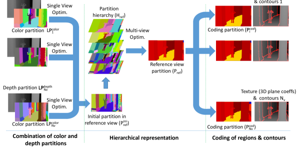
Figure 1: Overview of the multi-view optimal partition. Color & depth map images of multiple views are projected and combined in a reference view, where a hierarchy of regions is built (each layer shows a cut of the hierarchy). A Rate-Distortion optimization finds the optimal partition in the hierarchy which defines a coding partition in each of the input views. The coding partitions are used to encode the depth maps of each input view.

One of the problems of segmentation based coding systems is the high cost of sending the contours. In this work, we will assume that color images are already encoded and available at the decoder. Thus, depth boundaries can be approximated by a color partition without cost, because the color partition can be reproduced from the color image at the decoder. Only the approximation error (depth contours not present in the color image) will need to be explicitly sent, at a reduced coding cost.

The main contributions of this paper are:

• A consistent segmentation of the multiple views and a hierarchical representation of the different views.

• A new global scene representation based on a 3D planar model obtained from a hierarchical optimization.

• A method to efficiently encode the depth maps from multiple views, based on the global scene representation.

The outline of the paper is as follows. Related work in 3D planar representations and multi-view depth coding is studied in Section 2. In Section 3, the generic hierarchical optimization method is presented. In Section 4, the consistent multi-view depth map representation is introduced. Details of encoding the information of the multiple views are found in Section 5. Finally, we discuss the experimentation results and conclusion in Section 6 and Section 7 respectively.

2 Related Work

The use of 3D planar models to represent the structure of a scene has been explored in multiple applications. 3D planar models have shown to be useful to extract the structure of a scene using only color data in a stereo configuration Sinha et al (2009), to co-segment multiple view objects Kowdle et al (2012), to recover the structure of the scene from panoramic sequences Micusik and Kosecka (2009) or from a multi-camera environment Yin et al (2015). Multiple planes are detected and tracked in Time of Flight depth images using a layered scene decomposition in Schwarz et al (2011).

More similar to our configuration, in Barrera and Padoy (2014) the 3D point cloud from multiple RGB-D cameras is projected to the 3D world and used to generate a set of 3D planar patches consistent among the views. This patches are obtained with a Markov random fields using a voxelization of the scene and several 3D planar candidates. More recently, in Verleysen and De Vleeschouwer (2016) the same problem is tackled in a wide-baseline stereo configuration. Each image is segmented independently and a fitting process assigns a 3D plane to each region. Those planes are used as candidates in an energy-minimization problem, which optimizes the error of the model and the smoothness over neighboring regions.

Segmenting point clouds coming from RGB-D sensors has been tackled as a part of semantic labeling of indoor scenes and scene understanding. In Silberman et al (2012) a hierarchical segmentation is proposed using depth clues to infer the relations between objects and using priors to classify the different objects. In Ren et al (2012) an initial superpixel segmentation is used to compute kernel descriptors such as gradient, color and surface normal to build a hierarchy that is used to assign the labels to each node using markov random field. Gupta et al. Gupta et al (2013) generalize the gPb-ucm hierarchical segmentation to incorporate depth information for semantic segmentation. Lately, in Wang et al (2015) an unsupervised framework where joint feature learning and encoding is proposed for RGB-D scene labeling.

Planar models have been also proposed for depth representation on 3DTV applications. In Özkalaycı and Alatan (2014) a Markov random field model that mimics a Rate-Distortion trade-off is used in a stereo configuration to obtain a co-segmentation with planar approximations. A single reference MVD format is also proposed to fuse the information of the stereo views in a single reference.

Some depth map coding techniques propose improvements of the depth coding modes of 3D-HEVC. In Lucas et al (2015) an intra prediction framework with a flexible block partition scheme. Depth edges that cannot be predicted are explicitly encoded. Similarly, in Merkle et al (2016) a complete overhaul of the 3D-HEVC is defined. It incorporates planar signals to represent the smooth changes of flat scene areas, a new intra-picture prediction for this model and an improved wedgelet segmentation.

A joint color and depth coding for multi-view video is proposed in Gao et al (2016). Making use of DIBR, the color and depth information is projected obtaining a inter-view prediction. This inter-view prediction has missing pixels which are inpainted using minimum explicitly encoding.

In Maceira et al (2016) we proposed a region based coding of depth maps for a single-view. There we defined depth hierarchies to segment a depth map from one RGB-D image but only a flat partition was explored for coding. In the current paper we extend the depth hierarchies defined in Maceira et al (2016) to deal with multiple views on an optimal fashion.

3 Rate-Distortion hierarchy optimization

In this Section, we define a generic methodology to find the optimal partition in a hierarchy in terms of Rate-Distortion. The notation used is consistent with Varas et al (2015), where an optimization on multiple hierarchies is used for semantic segmentation of sequences. The optimization presents two benefits. Firstly, the encoding parameters are selected optimally for each region and secondly, the optimal final number of regions needed to encode the depth map can be automatically obtained. In this work, we will use this Rate-Distortion optimization in various steps of the proposed algorithm.

3.1 Hierarchy Definition

The representation of a hierarchy can be depicted with nodes as shown in Figure 2. Each node of the hierarchy represents a region in the image, and the parent node of a set of regions represents their merging. In all stages we assume that this hierarchy is binary (regions are merged by pairs). This structure is named as Binary Partition Tree Salembier and Garrido (2000). Commonly, such hierarchies are created using a greedy region merging algorithm that, starting from an initial leaf partition $LP$, iteratively merges the most similar pair of neighboring regions according to a region similarity criteria.

Figure 2: Hierarchical representation of an image. At each step the two most similar regions are merged.

The merging process ends when the whole image is represented by a single region, which is the root of the tree. The set of mergings that creates the tree, from the leaves to the root, is denoted as merging sequence (Figure 2). In a binary hierarchy, a merging sequence contains N partitions, where $N$ is the number of leaves (regions in $LP$). This is the set of partitions that is usually analyzed when working with hierarchies. Still, once the hierarchy is built, an analysis on the whole hierarchy could obtain partitions which are not included in the merging sequence (for instance, merging regions 3 and 5 in the example of Figure 2)

3.2 Rate-Distortion Problem Definition

The Rate-Distortion problem consists in finding the optimal coding that minimizes the distortion $D$ of the image with the constraint that the total cost $R$ is below a given budget Ortega and Ramchandran (1998). In our case, this optimal coding consists in finding the optimal partition to describe the image.

In a hierarchical representation, the Rate-Distortion function has to be defined (see Ortega and Ramchandran (1998)) with $R$ and $D$ additive measures in the hierarchy $H$:

$$R_{H}=\sum_{leaves}R_{k}$$ (1)

$$D_{H}=\sum_{leaves}D_{k}$$ (2)

Each node of the hierarchy can be encoded using a set of coding techniques generating a set of $R_{k}$ and $D_{k}$ for each region $k$. In this work, the distortion measure $D_{k}$ is computed as the Square Error between the estimated texture values and the real ones:

$$D_{k}=\sum\limits_{n=1}^{N_{k}}|\hat{g}(n)-g(n)|^{2}$$ (3)

where $N_{k}$ is the number of pixels of the region $k$, $g$ is the texture value of the pixels of the region and $\hat{g}$ is the estimated values with the texture coding option.

Typically, in region-based coding, two terms are needed to encode the region. The cost to store the position of the contours of the region $(R_{k}^{C})$ and the cost to store the texture coefficients $(R_{k}^{T})$. Hence, for each region their rate cost $R_{k}$ is defined as:

$$R_{k}=R_{k}^{C}+R_{k}^{T}$$ (4)

The constrained problem can be converted into an equivalent unconstrained one by using Lagrangian relaxation Ortega and Ramchandran (1998). Cost and distortion are combined using a positive multiplier $\lambda$ that defines the trade-off between the distortion allowed and the number of bits spent:

$$J_{k}=D_{k}+\lambda R_{k}$$ (5)

The best partition can be obtained by using a bottom-up local analysis at each node:

$$J_{parent}\leq J_{ch_{1}}+J_{ch_{2}}$$ (6)

where $J_{ch}$ is the cost of the cheapest path under the child node.

3.3 Hierarchy Optimization

The objective of the hierarchy optimization is to find the optimal boundary configuration that defines a partition using nodes from the hierarchy $H$ using the previously defined Rate-Distortion constraints.

Inspired by Charikar et al (2003); Glasner et al (2011); Varas et al (2015), we propose to solve the Rate-Distortion optimization problem as a quadratic semi-assignment problem (QSAP), restricting the solution to nodes of the hierarchy. Partitions are defined in terms of boundaries between regions and hierarchical constraints are added to solve the QSAP problem with a linear programming relaxation approach. The QSAP approach have two main advantages over other common approaches such as the dynamic programming solution. Firstly, QSAP defines the relation between regions (whether they are merged or not) in terms of their common contour. This relation allows to represent the contour cost of the union of two regions easily. Secondly, QSAP can be generalized to work with multiple hierarchies, which would allow applying the procedure defined in this work to relate frames of multiple time instants in order to remove temporal redundancy.

This optimization can be stated as a constrained minimization problem:

$$\min_{B}\ tr(QB)=\min_{B}\ \sum_{m,n}q_{m,n}b_{m,n}$$ (7)

$$s.t.\quad b_{m,n}\in\{0,1\}\ \forall m,n\ b_{m,m}=0$$

where matrix $Q$ is an affinity matrix that measures the quality of all the possible partitions in the hierarchy $H$. Matrix $B$ encodes those partitions as a binary matrix, where elements $b_{m,n}=1$ if the boundary between leaves $m$ and $n$ is active (regions $m$ and $n$ have not been merged) and $b_{m,n}=0$ otherwise.

In our case, the elements in matrix $Q$ can be defined to mimic the Rate-Distortion Lagrangian decision as:

$$q_{ch_{1},ch_{2}}=J_{parent}-(J_{ch_{1}}+J_{ch_{2}})$$ (8)

This allows to introduce the local node analysis of Equation (6) into the global framework optimization of Equation (7). The idea is that nodes with minimum Lagrangian $J$ are favored, thus leading to the optimal partition for a given $\lambda$. Figure 3 presents an example of Lagrangian optimization over the hierarchy presented in Figure 2. The algorithm examines all the nodes in the hierarchy (nodes 1-7) and selects the ones that present a minimum Lagrangian (nodes 3, 4 and 5). The final partition (shown in the right side of the figure) is composed of the regions represented by these nodes.

Figure 3: Example of Lagrangian optimization over the hierarchy presented in Figure 2. The optimization process activates the nodes with minimum Lagrangian $J$ (regions 3, 4 and 5), thus finding the best partition for a given $\lambda$.

The hierarchy $H$ contributes in two aspects to the optimization process. Firstly, it defines the mergings between regions of its leaves partition $LP$ to form clusters. Secondly, it also includes the order in which these regions should be merged to represent each node of the tree. As in Varas et al (2015), these restrictions are encoded using two coupled constraints per node. The first constraint imposes that all the variables representing boundaries between two siblings should have the same value. The second constraint imposes that for a given node, a variable representing a boundary between two siblings can only impose a merging if all the leaves associated with the node are merged.

The first constraint is defined as:

$$\sum_{n\neq l}^{m,n}b_{m,n}=(N_{c}-1)b_{m,l}$$ (9)

where $N_{c}$ is the total number of common region boundaries from the leaf partition that represents the union of both siblings, $m$ is a region from the first sibling and $n,l$ are regions from the second sibling.

The second as:

$$\sum^{n,l}b_{n,l}\leq N_{m}b_{m,o}$$ (10)

where $N_{m}$ is the total number of inner region boundaries from the leaves partition of both siblings, $m$ and $n$ are regions from the first sibling and $n,l$ are regions from the second sibling.

Adding these two constraints to the optimization process of Equation (7) results in:

$$\min_{B}\sum_{m,n}q_{m,n}b_{m,n}$$ (11)

$$s.t.\quad b_{m,n}\in\{0,1\}\quad b_{m,n}=b_{n,m}\quad\forall n,m$$

$$\sum_{n\neq l}^{m,n}b_{m,n}=(N_{c}-1)b_{m,l},\quad\sum^{n,l}b_{n,l}\leq N_{m}b_{m,o}\quad\forall p\in\{H\}$$

where $p$ represents any parent node in the collection of hierarchies. The result of this optimization is a binary matrix $B^{*}$ that describes the optimal partition $\{P^{*}(\lambda)\}$. Varying $\lambda$, different optimal Rate-Distortion partitions are found. Each $\lambda$ corresponds to a different potential solution on the convex hull of the operational Rate-Distortion points. It can be demonstrated that the set of solutions is finite Shoham and Gersho (1988). Because of the monotonicity of $R(\lambda)$, only a small subset of $\lambda$ need to be searched and the convergence of the algorithm is ensured in all cases.

4 Multi-view 3D Representation

The proposed multi-view depth map coding system fuses the information of multiple views in a unique 3D representation. Our method builds a 3D representation from a set of initial 2D partitions for each of the views. The global scheme is depicted in Figure 4. It starts by finding a partition for each individual view $i$ which merges color and depth partitions optimally, reducing the computational complexity of the multi-view process. The single-view processing is done independently for each view as shown in Figure 5 and explained in Section 4.1.

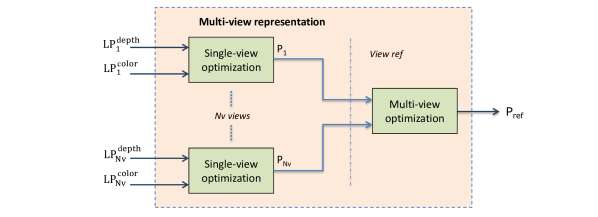
Figure 4: Multi-view representation. For each view $i$, a joint color and depth optimization finds a $P_{i}$ partition. The $N_{v}$ $P_{i}$ partitions are projected to the reference view where a multi-view optimization finds the best set of regions for each partition.

The information of the multiple views is accumulated in the reference view $view_{ref}$ by projecting the views partitions into $view_{ref}$. Then, an optimization process (depicted in Figure 8) obtains $P_{ref}$ which defines the final coding partitions for each view. Complete details on this process are given at Section 4.2.

We refer the optimization process of Equation (11) as:

$$P^{*}(\lambda)=Opt_{\lambda}(H)$$ (12)

where for a given $\lambda$ an optimal partition $P^{*}$ is extracted from $H$. For simplicity, we will reduce the notation of optimal partitions from $P^{*}(\lambda)$ to $P$.

In this work we use the initial color and depth leaves partitions from Maceira et al (2016). We name those initial partitions as $LP^{color}_{i}$ and $LP^{depth}_{i}$ respectively. Hierarchies in the single-view and the multi-view stages are built as in Maceira et al (2016): region contents are projected into 3D and modeled as 3D planes with RANSAC Fischler and Bolles (1981). The merging criterion is based on 3D plane similarity. Both stages find optimal partitions $P^{*}$ inside the hierarchy with the method presented in Section 3.

4.1 Single-View Optimization

In the Single-View Optimization $LP^{color}_{i}$ and $LP^{depth}_{i}$ are combined into an optimal partition $P_{i}$ for each view $i$ as shown in Figure 5.

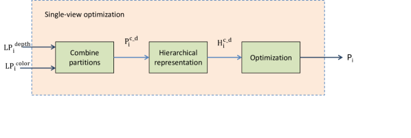
Figure 5: Optimization process for each view. A combined color and depth optimization is performed finding an optimal combined partition.

$LP^{color}_{i}$ and $LP^{depth}_{i}$ are fused into a partition $P^{c\_d}_{i}=LP^{color}_{i}\bigcap LP^{depth}_{i}$ that preserves all the boundaries from both partitions. The $P^{c\_d}_{i}$ is used to build a hierarchy $H^{c\_d}_{i}$. The optimization procedure introduced in Section 3.2 over that hierarchy obtains an optimal Rate-Distortion partition $P_{i}$:

$$P_{i}=Opt_{\lambda}(H^{c\_d})$$ (13)

For each view $i$, Equation (8) can be expressed as follows:

$$q_{ch_{i,1},ch_{i,2}}=J_{p_{i}}-(J_{ch_{i,1}}+J_{ch_{i,2}})=$$ (14)

$$(D_{p_{i}}+\lambda R_{p_{i}})-(D_{ch_{i,1}}+\lambda R_{ch_{i,1}})-(D_{ch_{i,2}}+\lambda R_{ch_{i,2}})=$$

$$\triangle D_{ch_{i,1},ch_{i,2}}+\lambda\triangle R_{ch_{i,1},ch_{i,2}}$$

where $p_{i}$ is the parent region resulting of the union of children $ch_{i,1}$ and $ch_{i,2}$:

$$p_{i}=ch_{i,1}\bigcup ch_{i,2}$$ (15)

$\triangle D_{ch_{i,1},ch_{i,2}}$ is the increment in distortion caused by the union of Equation (15) while $\triangle R_{ch_{i,1},ch_{i,2}}$ is the increment in rate of this union. Typically, the $\triangle D_{ch_{i,1},ch_{i,2}}$ is positive as representing the depth map with less regions will increase the distortion and $\triangle R_{ch_{i,1},ch_{i,2}}$ is negative.

The distortion of each region $k$ of the hierarchy is computed as the square error between the 3D planar model and the pixel values of the region, particularizing Equation (3) as:

$$D_{i,k}=\sum\limits_{n=1}^{N_{i,k}^{Pix}}|Proj_{i}(\Pi_{k},n)-g_{i}(n)|^{2}$$ (16)

where $\Pi^{3D}_{k}$ is the plane model for region $k$, $N_{i,k}^{Pix}$ is the number of pixels of region $k$, $Proj_{i}(\Pi_{k},n)$ is the value of the projected 3D planar model to the pixel $n$ of region $k$ and $g_{i}(n)$ is the depth value of pixel $n$ for each view $i$. An example of the projection step is shown in Figure 6.

The $\triangle D_{ch_{i,1},ch_{i,2}}$ is computed as:

$$\triangle D_{ch_{i,1},ch_{i,2}}=D_{p_{i}}-D_{ch_{i,1}}-D_{ch_{i,2}}$$ (17)

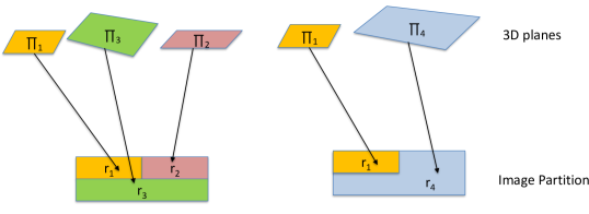
Figure 6: The Single-View distortion is computed projecting each 3D planar model to all the pixels of the corresponding region. The $r_{4}$ distortion generated with $\Pi_{4}$ is compared with a representation using the child regions $r_{2}$ and $r_{3}$, represented with models $\Pi_{2}$ and $\Pi_{3}$.

To compute the $\triangle R_{ch_{i,1},ch_{i,2}}$ two terms are present: texture and contour. For texture:

$$\triangle R^{T}_{ch_{i,1},ch_{i,2}}=R^{T}_{p_{i}}-R^{T}_{ch_{i,1}}-R^{T}_{ch_{i,2}}=-R^{T}$$ (18)

since the cost of texture is constant ($R^{T}$) for all regions.

Contours of a region may come from two partitions; some from $LP^{color}_{i}$ and some from $LP^{depth}_{i}$. The contour cost $\triangle R_{ch_{i,1},ch_{i,2}}^{C}$ is computed by counting the number of contour elements (two neighboring pixels with different labels define one contour element between them) of the regions $ch_{i,1}$, $ch_{i,2}$ and multiplying for the average cost of encoding each contour element. Since we are considering the common contours, the contour cost for the parent is zero. Then:

$$\triangle R_{ch_{i,1},ch_{i,2}}^{C}=-c_{A}\,N_{ch_{i,1},ch_{i,2}}-c^{\prime}_{A}\,N^{\prime}_{ch_{i,1},ch_{i,2}}$$ (19)

where $N_{ch_{i,1},ch_{i,2}}$ and $N^{\prime}_{ch_{i,1},ch_{i,2}}$ are the numbers of common contours of the two children from the depth and color partitions respectively, while $c_{A}$ and $c^{\prime}_{A}$ are the average costs to encode a contour element for either the depth and the color partitions. Note that contours from the color partition do not introduce any cost, therefore $c^{\prime}_{A}=0$. The $c_{A}$ has been obtained experimentally using the multi-view sequences resulting in $c_{A}$ = 1.2 bits per contour position.

Equation (4) is computed as:

$$\triangle R_{ch_{i,1},ch_{i,2}}=\triangle R_{ch_{i,1},ch_{i,2}}^{C}+\triangle R_{ch_{i,1},ch_{i,2}}^{T}=-c_{A}\,N_{ch_{i,1},ch_{i,2}}-R^{T}$$ (20)

Figure 7 shows an example of merging two regions. Encoding $r_{4}$ instead of $r_{2}$ and $r_{3}$ saves the cost of encoding the boundary between the regions and the texture coefficients of one region.

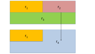
Figure 7: The Single-View rate for each region is the rate saving promoted by the merging. Regions $r_{2}$ and $r_{3}$ are merged into $r_{4}$, leading to represent the depth map without the contour between $r_{2}$ and $r_{3}$ and saving one 3D plane.

The color-depth optimization in each view addresses the addition of the depth boundaries in the color partition in an optimal fashion while reducing heavily the total number of regions. Doing this procedure in each view also reduces the number of occluded regions in the Multi-View Optimization.

4.2 Multi-View Optimization

The multi-view optimization process is shown in Figure 8. The partition $P_{i}$ of each of the $N_{v}$ views is projected, using the camera parameters, to $view_{ref}$, obtaining an initial partition $P_{i}^{\,ini}$ for each view $i$:

$$P_{i}^{\,ini}=Proj_{ref}(P_{i})$$ (21)

Pixels in each partition $P_{i}$ are processed in scan order and the corresponding pixel labels are projected to $view_{ref}$. Each individual projected partition $P^{ini}_{i}$ is defined by assigning to each pixel position the label of the nearest projected view $i$ pixel. With this process the regions that are near to the camera position prevail over the ones that are further away.

In this projection step, regions of view $i$ that are occluded in the reference view are detected. A region is considered occluded if the number of pixels of this region in $view_{ref}$ is less than half the number of pixels in view $i$. Occluded regions have no valid correspondence in $view_{ref}$. To solve this, these regions will be encoded independently in that view and removed from the projected partition in $view_{ref}$.

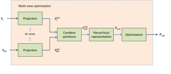
Figure 8: Multi-View Optimization process for each view. Partitions from multiple views are combined in a unique hierarchy. Rate-Distortion measures are computed using all the input views and stored in the hierarchy to find the joint optimal partition for the multiple views.

The individual projected partitions $P^{ini}_{i}$ in $view_{ref}$ are accumulated in a unique partition as stated in Equation (22). Unlike the single-view optimization, here in the projected $view_{ref}$ not all the pixels have a projected label. In order to obtain a partition with all the pixels assigned to a label, a hole filling algorithm creates new labels in-between regions with different label. For each combination of labels in each $view_{i}$, a new label is created in $P^{ini}_{ref}$.

$$P^{ini}_{ref}=\bigcap_{i}P^{ini}_{i}$$ (22)

A hierarchical depth representation $H_{ref}$ is built using the accumulated partition $P^{ini}_{ref}$. Rate and distortion values for each region in $H_{ref}$ are found examining each partition generated in the $N$ views. The increment of distortion for each union is computed as:

$$\triangle D_{ch_{1},ch_{2}}=\sum\limits_{i=1}^{N}\triangle D_{ch_{i,1},ch_{i,2}}$$ (23)

where $\triangle D_{ch_{i,1},ch_{i,2}}$ represents the increment of distortion of each view $i$ as in Equation (17). A graphical example of Equation (23) is shown in Figure 9. Notice that, in the example, $r_{ocl\,1}$ is occluded in $view_{ref}$. Therefore, $r_{ocl\,1}$ does not participate of the optimization process and is encoded with a independent plane.

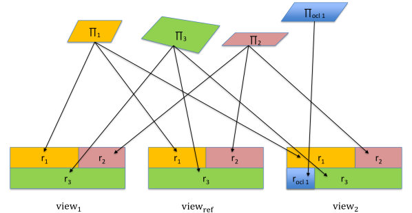
Figure 9: The Multi-View distortion is computed projecting each 3D planar model to all the pixels of the corresponding region of each image.

Similarly, the rate is computed using the information of all views, adding the boundary cost (from depth boundaries only, as $c^{\prime}_{A}=0$ for color contours):

$$\triangle R_{ch_{1},ch_{2}}=\sum\limits_{i=1}^{N}\triangle R_{ch_{i,1},ch_{i,2}}$$ (24)

As the same region model encodes regions of multiple views, the texture rate is the same than in the single view optimization:

$$\triangle R_{ch_{1},ch_{2}}=-c_{A}\,\sum\limits_{i=1}^{N}N_{ch_{i,1},ch_{i,2}}-R^{T}$$ (25)

An example of computing the rate for the Multi-View optimization is shown in Figure 10.

The $P_{ref}$ partition is obtained using the hierarchical optimization of Section 3.2:

$$P_{ref}=Opt_{\lambda}(H_{ref})$$ (26)

Since the hierarchy $H_{ref}$ is build in the $view_{ref}$, the merging orders are determined in $view_{ref}$. By incorporating the information of the $N_{v}$ views to the optimization process, the resulting partition $P_{ref}$ defines an optimal partition in all the views.

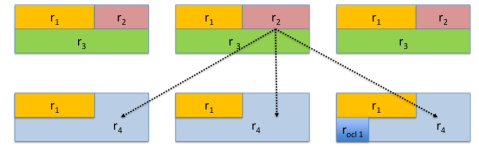
Figure 10: The Multi-View rate for each region is the rate saving obtained with the merging. A merging in $view_{ref}$ may force a merging in the other views.

The optimization parameter $\lambda$ that defines the Rate-Distortion trade-off is the quality parameter. By varying $\lambda$, different Rate-Distortion points are found, being able to obtain 3D scene representations with different level of detail.

5 Multi-view depth map coding

In Section 4, the proposed method to obtain a joint segmentation of the scene combining color and depth partition has been explained. In order to convey the depth information to the decoder we propose a method to pack the information of the multiple views efficiently. The method assumes that the camera parameters and the color images of each view have been encoded and sent to the decoder before decoding the depth map information. The partition $P_{ref}$ is projected back, following the inverse process of Equation (21), to obtain a consistent set of coding partitions $P^{cod}_{i}$ for each of the $N_{v}$ views.

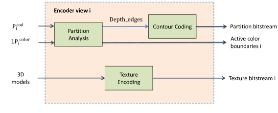
Figure 11: Encoder scheme. Partition information is generated independently for each view. Texture encoding encodes the 3D plane in INTRA if it is the first view where it appears or INTER if it has been encoded previously.

The general coding scheme for each view $i$ is presented in Figure 11. The first step consists in analyzing which contours from $LP^{color}_{i}$ and $LP^{depth}_{i}$ are present in $P^{cod}_{i}$. Contours in $P^{cod}_{i}$ from $LP^{depth}_{i}$ are encoded with Freeman contour coding Freeman (1961) independently for each view. For the color contours, information of color boundaries that are not active (because of region mergings) is sent to the decoder indicating if the merging has been done or not. Active information is stored with 1 bit per each merging in $H_{ref}$.

Once the partition information has been encoded, the texture coefficients are generated. The first view encodes the texture information of all the planes associated to that view in INTRA mode, while planes from the subsequent views will be encoded using INTER view prediction when possible. In the INTRA mode, the 3D planes are represented by using the distance of that plane to a camera plus the plane orientation. This plane orientation is stored in spherical coordinates with their 3D angles $\theta$ and $\phi$:

$$\theta=arccos\left(\frac{n_{z}}{\|n\|}\right)\qquad\phi=arctan\left(\frac{n_{y}}{n_{x}}\right)$$ (27)

where the $n_{z}$ component is pointed towards $z>0$. The resulting angles (in the range $0\leq\theta\leq\frac{\pi}{2}$ and $0\leq\phi\leq 2\pi$) are encoded with equal precision with a uniform quantizer.

The distance from the plane to the camera is converted to an alternative quantized representation using the distance to depth map conversion:

$$C_{dist}=\frac{1.0}{\frac{d(pl,c)}{(2^{N_{dist}}-1)}*(\frac{1.0}{MinZ}-\frac{1.0}{MaxZ})+\frac{1.0}{MaxZ}}$$ (28)

where $d(pl,c)$ is the euclidean distance between the region plane and the camera, $N_{dist}$ is the number of bits to be used in the quantization and $MaxZ$ and $MinZ$ are the maximum and minimum depth values of the image.

For subsequent views $i$, the INTER mode is used. Planes from the first view are projected to view $i$ as done in the construction of the multi-view partition in $view_{ref}$. Each region in view $i$ has a candidate plane from the first view. This plane is compared with a plane coded with INTRA in view $i$. The plane with the lower error is kept. If the plane is coded with INTER, a SKIP mode is sent, if not the region is INTRA coded.

The bitstream (depicted in Figure 12) provides the decoder with the information needed to recover the partition and the texture for each region. The partition bitstream, active color boundaries and texture bitstream for each view are provided in addition of the number of regions $N_{regs\_color}$ in each initial color partition $LP^{color}_{i}$. $N_{regs\_color}$ is the same for the $N_{v}$ views.

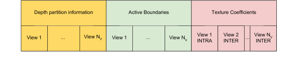
Figure 12: Bitstream with the information of the $N_{v}$ views. The depth partition information signal the depth boundaries added to the color information. With the active boundaries information the final coding partition is obtained. The texture coefficients for views 2 to $N_{v}$ make use of the previous transmitted coefficients.

The decoder process is depicted in Figure 13. For each view, the $LP^{color}_{i}$ is built from the decoded color image. From that partition, color edges are removed using the active color boundaries information. Then new edges are added from the partition bitstream. Depth map is recovered by decoding the texture bitstream and projecting each 3D plane to $P^{cod}_{i}$.

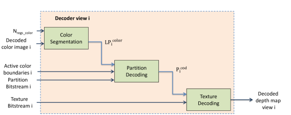
Figure 13: Decoder scheme. $LP^{color}_{i}$ is generated from the decoded color image using $N_{regs\_color}$. Using the information of active color boundaries and the partition bitstream the encoding partition $P^{cod}_{i}$ is generated. The decoded depth map for view i obtained by projecting the 3D planes to $P^{cod}_{i}$.

6 Experimental Evaluation

In this section, we present a quantitative evaluation of our multi-view optimization segmentation and coding method. We use the RGB-D multi-view sequences Ballet, Undo Dancer, Breakdancers and Ghost Town for evaluation Zitnick et al (2004); Zhang et al (2011); Rusanovskyy et al (2011). Each sequence is composed of color and depth frames from up to $8$ camera views as well as camera parameters for each frame. Ballet and Breakdances have been captured using color (RGB) cameras and the depth has been computed afterwards. Undo Dancer and Ghost Town are synthetic sequences. The resolution of the sequences is 1920x1088 pixels for Undo Dancer and Ghost Town and 1024x768 pixels for Ballet and Breakdancers. We assume that color views have been previously decoded at the receiver side. The different stages of the proposed method are evaluated using $25$ frames of each sequence.

In order to assess our technique, we first explore different configurations of the proposed method in Section 6.1. Finally, our proposal is compared against HEVC, 3D-HEVC and MV-HEVC in Section 6.2.

Experiments will make use of three views: $view_{left}$, $view_{right}$ and $view_{ref}$ using the same configuration of 3D-HEVC. $view_{left}$ and $view_{right}$ are the two base views to encode and $view_{ref}$ is the location selected to perform the optimization process in the multi-view optimization block (See Section 4.2). This view corresponds to the virtual view of 3D-HEVC. Color and depth map images as well as the camera parameters are available in the three views considered.

6.1 Configuration

In this Section, the different blocks of the overall system are analyzed. The first experiment studies how the number of views affects the coding performance of our method. Then, we show the gain of using the RD optimization in the hierarchy. In the third experiment, we show the difference between using a color partition or a combination of color plus depth partitions. Finally we study the distribution of rate among depth partition information, active boundaries and texture coefficients. Results for the different sequences are averaged into a single Rate-Distortion curve.

Combining multiple views

In this experiment we study the combination of several views prior to the multi-view optimization

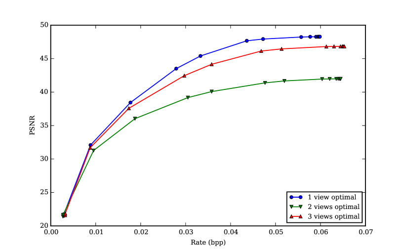
Figure 14: Coding results in the $view_{ref}$. 1 view configuration has only information of $view_{ref}$, 2 view configuration use the 2 views projected to $view_{ref}$ and 3 view configuration uses the three of them.

Figure 14 shows the results of encoding the $view_{ref}$ depth map in different configurations. In each configuration, a different number of views is used to obtain the hierarchy in $view_{ref}$.

In the 1 view optimal configuration, only information from the $view_{ref}$ is used. This configuration is the one that achieves better Rate-Distortion figures. The 2 views optimal configuration uses information of $view_{left}$ and $view_{right}$. As the projection from those views to $view_{ref}$ is not able to match all the depth boundaries in $view_{ref}$, the results for the 2 views optimal are below the 1 view configuration. With the 3 views optimal all 3 views are used. Results are slightly below the 1 view optimal, but in this case we optimize for the 3 views together, obtaining a consistent segmentation across the views.

The resulting optimal coding partitions for each configuration are projected back to $view_{left}$ and $view_{right}$, as presented in Section 5. Results are shown in Figure 15. The different configurations achieve similar results, all of them below the results of the single-view configuration. This behavior is due to the fact that the hierarchical optimization in $view_{ref}$ restricts the possible mergings in the other views and that an extra rate is needed to encode occluded regions.

With the Single-View optimization, the number of regions in the different views is reduced before building the shared hierarchy between views in $view_{ref}$. Being able to merge regions in a single-view reduces the number of regions that are occluded in $view_{ref}$ while creating a hierarchy $H_{ref}$ in $view_{ref}$ with relevant regions.

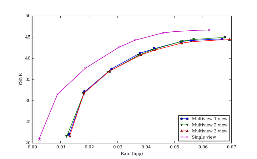
Figure 15: Results from Figure 14 are translated to $view_{left}$ and $view_{right}$. The three multi-view configuration (all with hierarchy built in $view_{ref}$) are compared with a hierarchy in each view independently.

Rate-Distortion optimization

In this Section, the performance of the Rate-Distortion optimization method in the Single-View Configuration is studied. Different cuts of the hierarchy $H^{c\_d}_{i}$ (this is, different partitions) extracted following the merging sequence are compared with optimal partitions $P_{i}$ with different quality parameter $\lambda$. Results are shown in Figure 16. By using the proposed optimization, we are able to achieve a gain of 2-3 dB over using the $H_{i}^{depth}$ merging sequence.

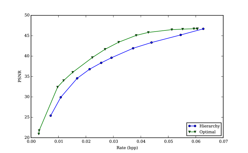
Figure 16: Rate-Distortion results with the proposed optimization method. Using an initial $H^{depth}$, results from coding the partition with 3D planes following the merging sequence and with the proposed optimization.

Color and depth combination

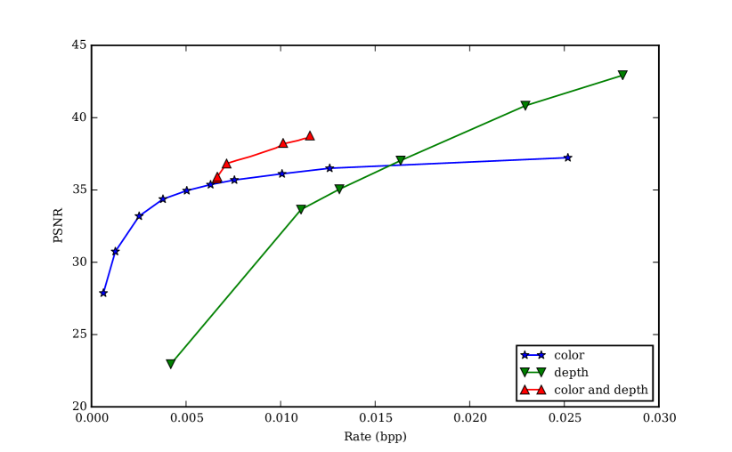
Figure 17: R-D curves using color partitions, depth partitions and combined color and depth partitions to encode depth maps. Partitions using depth include the cost of encoding texture and boundary while the colors only need texture information.

Figure 17 shows the R-D curves for three different options: using only a depth partition, using only a color partition and using a color-depth partition. Using only color partition has the advantage that no contour information has to be sent. It’s a good option for very low bit-rates but the lack of precision in the region boundaries limits the maximum achievable quality. Using only depth information allows to obtain higher quality as all the contours have to be sent, the curve is displaced to the right. The combination of color and depth provides a good trade-off because most of the depth contours can be approximated using color boundaries and only a reduced set of depth contours not present in the color partition must be sent.

Multi-view optimization: rate statistics

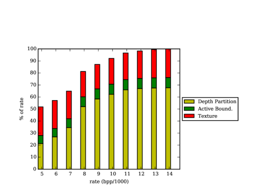
Figure 18: Distribution of rate in texture, partition and active boundaries information for different Rate-Distortion points.

To evaluate the distribution of rate among depth partition information, active boundaries and texture coefficients, the bitstream presented in Section 5 was analyzed to determine the different contributions. Figure 18 shows the rate distribution among each category. Each bar is normalized with the maximum rate in the last column. The cost of encoding the texture and the information of active boundaries remains fairly constant among all the different Rate-Distortion points. However, the partition cost becomes the prevailing one as the rate increases. The results of the optimization depend on the given budget rate. When the budget is low, only color boundaries are added. When more bits can be allocated, the optimization adds the costly depth boundaries.

6.2 Rate-Distortion results

As the proposed method does not have temporal prediction, only intra modes for the different methods are taken. For each sequence, three views are used, $view_{left}$ and $view_{right}$ are encoded (each view independently) and the middle one is employed as the location for the $view_{ref}$. The view rendered using the original depth maps serves as a reference for the different methods in the virtual view.

To objectively evaluate the proposed method, error measures are taken both in the depth map and in the synthesized virtual view. Since depth maps are not visualized but used to render new images, the measure in the virtual view gives the real performance of the method. Measuring directly on the depth map gives an overview of how the original depth map can be represented with planes. Similar results were obtained using PSNR and SSIM. As both measures show similar tendencies, only the PSNR will be shown to evaluate the error.

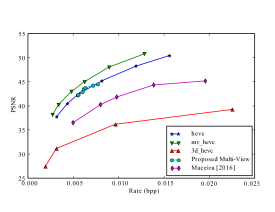
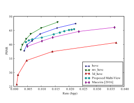
a) Undo Dancer	b) Ghost Town
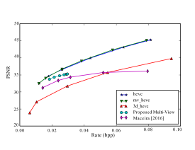
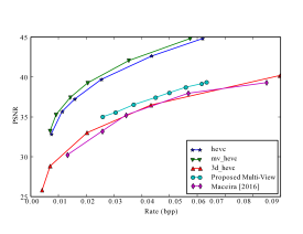
c) Ballet	d) Breakdancers

Figure 19: Rate distortion results evaluated directly in depth maps.

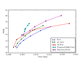
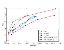
a) Undo Dancer	b) Ghost Town
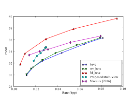
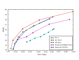
c) Ballet	d) Breakdancers

Figure 20: Rate distortion results evaluated over rendered views.

Results measured on the depth map for the different sequences are shown in Figure 19. In that comparison, the 3D-HEVC performs worse than the other HEVC configurations methods of the literature. This is because color and depth map for two views are encoded together in 3D-HEVC, the view synthesis optimization maximize the quality in the virtual view and not directly in the depth map. The proposed method outperforms Maceira et al (2016) ([Maceira2016]) for all the sequences. The use of multi-view redundancy as well as the proposed optimization net allows a more than 2 dB gain for the different sequences. This improvement is noteworthy for the Undo Dancer sequence, where the planar characteristic of the scene can be fully exploited. On the other hand, our method has more problems with the Ghost Town sequence, where the number of added depth contours is similar to Maceira et al (2016), thus achieving similar results. This is because the color segmentation is not able to properly segment elements at different depths since all of them have the same tonality.

In sequences where the depth map is noisier, as Ballet and Breakdancers, the 3D planar segments are not able to represent correctly the depth maps, thus obtaining worse results than the HEVC standards.

Results in the rendered virtual view are shown in Figure 20. The results of the planar implementations achieve better results than HEVC and MV-HEVC in Ballet and Undo Dancer and are closer than in the depth map comparison in the other sequences. Notice that in Undo Dancer 3D-HEVC does not improve HEVC or MV-HEVC. This is due to 3D-HEVC encoding together color and depth information. Here we only take the depth maps from the 3D-HEVC, using the same color image than the other methods for doing the rendered view. The results for Figure 20 are summarized in Tables 1 and 2 where the Bjontegaard’s metric to compute the average gain in psnr (BD-SNR) and to compute the average saving in bitrate (BD-Rate) are shown, taking the HEVC as a reference.

Table 1: BD-RATE

	MV-HEVC	3D-HEVC	Maceira2016	Proposed
Undo Dancer	-23.69	-40.97	-36.94	-49.16
Ghost Town	-39.96	-64.50	42.03	2.91
Ballet	-6.03	-71.89	-37.16	-41.63
Breakdancers	-6.16	-35.71	48.46	150.13

Table 2: BD-SNR

	MV-HEVC	3D-HEVC	Maceira2016	Proposed
Undo Dancer	1.16	1.80	2.12	3.38
Ghost Town	1.43	2.16	-1.03	0.01
Ballet	0.20	3.47	1.57	1.51
Breakdancers	0.17	1.02	-1.03	-2.57

The multi-view method proposed improves the Rate-Distortion results of Maceira et al (2016) for all sequences, achieving encoding results competitive with the HEVC standards. However, this result is not translated equally in virtual views. For instance, Ballet and Breakdancers sequences are noisier and present a larger baseline between views. In this case, the proposed method reduces the number of 3D planes when encoding the corresponding depth maps, which penalizes the performance of the method. On the other hand, in sequence Undo Dancer, the planar characteristics of their depth maps allow an improvement over the HEVC standards. In addition, the multi-view method presented in this work extracts a consistent segmentation for the different views, which could be very useful in further applications.

7 Conclusion

In this work we have presented a region-based multi-view depth map coding technique based on a global 3D scene representation. Color and depth segmentations of the different views are combined into a single hierarchical representation. An optimization process over this hierarchy allows to obtain the optimal coding partition. This representation retrieves a unique 3D planar decomposition of the scene. A method to encode the 3D planar decomposition for multi-view depth map coding application is also proposed. Texture information is sent by modeling each resulting region as a 3D plane and sending the corresponding plane parameters. The use of a color partition (that is already available at the decoder, without extra cost) allows to reduce the cost of sending this coding partition. The multi-view coding method shows competitive results against HEVC.

A side benefit of the proposed method is that, in addition to coding, the global 3D scene representation is susceptible to be used in tasks such as action detection Liang and Zheng (2015), scene recognition Gupta et al (2013) or scene labeling Wang et al (2015).