A Machine Learning Based Source Property Inference for Compact Binary Mergers

Abstract

The detection of the binary neutron star (BNS) merger, GW170817, was the first success story of multi-messenger observations of compact binary mergers. The inferred merger rate along with the increased sensitivity of the ground-based gravitational-wave (GW) network in the present LIGO/Virgo, observing runs, strongly hints at detections of binaries which could potentially have an electromagnetic (EM) counterpart. A rapid assessment of properties that could lead to a counterpart is essential to aid time-sensitive follow-up operations, especially robotic telescopes. At minimum, the possibility of counterparts require a neutron star (NS). Also, the tidal disruption physics is important to determine the remnant matter post merger, the dynamics of which could result in the counterparts. The main challenge, however, is that the binary system parameters such as masses and spins estimated from the realtime, GW template-based searches are often dominated by statistical and systematic errors. Here, we present an approach that uses supervised machine-learning to mitigate such selection effects to report possibility of counterparts based on presence of a NS component, and presence of remnant matter post merger in realtime.

1 Introduction

The first two observing runs of the LIGO detectors, (Aasi et al., 2015) and the Virgo detector (Acernese et al., 2014) witnessed remarkable level of participation from the electromagnetic (EM) astronomy community in search for EM counterparts of gravitational wave (GW) detections from coalescing binaries (Abbott et al., 2019a, b). As the detectors become more sensitive, the projected detection rates of such events will increase (Abbott et al., 2018). Technological improvement is not just confined to GW detectors alone. Current and upcoming telescope facilities such as the Zwicky Transient Facility (Kulkarni, 2016) and the Large Synoptic Survey Telescope, (Ivezić et al., 2008) consistent with the timeline of LIGO/Virgo operations, plan to participate in the follow-up efforts (see Graham et al. (2019), for example).

Observers are interested to know about the presence of a neutron star (NS) in coalescing binaries. This is a minimum condition for there to be matter post merger. The dynamics of matter in the extreme environment of the aftermath of a compact binary merger is responsible for EM phenomena associated with GWs. Binary black hole (BBH) mergers, therefore, are not expected to have an associated counterpart, since they are vacuum solutions to the Einstein’s field equations. Even in the presence of a NS, other effects, like the equation of state (EoS) of the NS(s), or the mass and spin of the companion BH plays crucial role in the tidal disruption, and the amount of matter ejected. For a neutron star black hole (NSBH) system, tidally disrupted material from the NS could form an accretion disk around the central BH. High temperatures in the disk could lead to annihilation of neutrinos to pair produce electron-positrons, which further annihilate to power a short GRB. This could also happen via extraction of rotational energy from the BH due to the presence of magnetic field lines threading the BH horizon (Blandford & Znajek, 1977). In the case of unbound ejecta, $r$-process nucleosynthesis can power a kilonova. (Lattimer & Schramm, 1974; Li & Paczyński, 1998; Korobkin et al., 2012; Tanaka & Hotokezaka, 2013; Barnes & Kasen, 2013; Kasen et al., 2015) For a binary neutron star (BNS) system, even if the tidal interaction is not strong enough, the two bodies will eventually come into physical contact, resulting in shocks that expel neutron rich material. This will result in a kilonova as seen in the case of GW170817 (Abbott et al., 2017; Arcavi et al., 2017; Coulter et al., 2017; Kasliwal et al., 2017; Lipunov et al., 2017; Soares-Santos et al., 2017; Tanvir et al., 2017). The interaction of the ejecta with the surrounding medium can result in synchrotron emission, observable in X-rays and radio in weeks to months. There can be relativistic outflows, which could result in a GRB, as seen for GW170817; although, there could be cases of prompt collapse where GRB generation could be suppressed (Ruiz & Shapiro, 2017). Nevertheless, the generation of some EM messenger is highly probable. Therefore, data products that predict the existence of matter is useful in the EM counterpart follow-up operations.

An accurate computation of the remnant matter requires general-relativistic numerical simulations of compact mergers. These are expensive, and only a few ($\lesssim 100$) such simulations have been performed to date. Also, such a simulation is not possible in the time scale of discovery, and generic target of opportunity follow-up of GW candidates. Empirical fits to the numerical relativity results, however, have been performed, and are a use case for such realtime inferences. For example, Foucart (2012) and Foucart et al. (2018) devised an empirical fit to predict the combined mass from the accretion disk, the tidal tail, and the ejecta remaining outside the final BH in case of a NSBH merger. However, it should be mentioned that such fits often require more input than what is available from the realtime GW data. For example, the fits mentioned above require the compactness of the NS, which is not a parameter inferred by the GW searches. The NS EoS, which is not constrained strongly, is to be assumed in order to infer the compactness.

The second LIGO/Virgo observing run, O2, saw the first effort to provide realtime data products to aid EM follow-up operations from ground and space based facilities (Abbott et al., 2019a). These included sky localization maps, (Singer & Price, 2016; Singer et al., 2016) and source classification of the binary which included

1. the probability that there was at least one neutron star in the binary, $p(\texttt{HasNS})$, and

2. the probability that there was non-zero remnant matter, $p(\texttt{HasRemnant})$, considering the mass and spin of the components, based on the Foucart (2012) fit.

For a BNS merger, we expect some matter to be expelled (see Table 1 of Shibata & Hotokezaka (2019) for different scenarios). Therefore, we expect the result, $p(\texttt{HasNS})=1$; $p(\texttt{HasRemnant})=1$. On the other extreme, BBH coalescences will not lead to remnant matter, since they are vacuum solutions, i.e., $p(\texttt{HasNS})=0$; $p(\texttt{HasRemnant})=0$. Hence, $p(\texttt{HasRemnant})$ is more relevant for NSBH systems. Here, the mass and spin of the BH determines the tidal disruption of the NS. Lower mass, and high spin implies a smaller innermost stable circular orbit which allows the NS to inspiral closer to BH. The tidal force exerted by the BH, which also increases with spin, then tears the NS apart. This leaves remnant matter post merger. However, if the NS is compact, or tidal forces are not sufficient enough, the NS is swallowed whole into the BH, leaving no remnant. The type and morphology of EM counterparts generated depends on the amount of matter ejected and its properties. Pannarale & Ohme (2014) considered the conditions for short GRB production in the context of LIGO/Virgo observations of NSBHs. More recent work has tried to understand the morphology of kilonovae from NSBH mergers considering the density structure of the ejected matter, opacity properties, the viewing angle, and other factors (see Barbieri et al. (2019); Hotokezaka & Nakar (2019), for example). However, accurate modeling is still at its infancy. Thus, the presence of remnant matter is a conservative proxy for the presence of counterparts, still more constraining than the presence of a NS component alone, albeit the model dependence i.e., the assumption of NS EoS, and the usage of a particular fit. The rationale behind computing two quantities is to give flexibility to observing partners in follow-up operations.

The main challenge in this inference, however, is to handle detection uncertainties in the parameter recovery of the realtime GW template-based searches. This was done in O2 via an effective Fisher formalism using an ambiguity region around the parameters of the triggered template. The algorithm used for O2 is described in Sec. 3.3.2 of Abbott et al. (2019a), and briefly summarized in Sec. 2 below. While it accounted for statistical uncertainties, the systematic errors in the low-latency GW template based analysis were not considered. Here we consider the problem differently. We treat the problem as binary classification, and present a new technique that is based on supervised learning. This not only improves the speed and accuracy, but also removes runtime dependencies that were required during O2 operations. Also, this technique provides flexibility to incorporate astrophysical rates of binary populations in the universe.

In the third LIGO/Virgo observing run, O3, these data products (and a few more) continue to be part of the public alerts. In this work, we make a slight modification to the nomenclature. The $p(\texttt{HasRemnant})$ quantity had been referred to as EM bright classification probability in Abbott et al. (2019a). Here, we refer to the both these quantities collectively as source properties, following the O3 LIGO/Virgo public alert userguide. These values indicate the chances of the matter remaining post merger, the dynamics of which can launch EM counterparts. For example, the combination $p(\texttt{HasNS})=1$; $p(\texttt{HasRemnant})=0$, indicates a conservative measure of presence of matter – just the presence of NS. However, the combination $p(\texttt{HasNS})=1$; $p(\texttt{HasRemnant})=1$, is a stronger indication of the presence of a counterpart, albeit some model dependence.

The organization of the paper is as follows. In Sec. 2 we provide a brief review of the ellipsoid-based inference used in O2. In Sec. 3, we present the inference using a supervised learning method called KNeighborClassifier (Pedregosa et al., 2011), which was trained on injection campaigns from the GstLAL search pipeline (Messick et al., 2017) used by LIGO/Virgo in routine search sensitivity analyses during O2. We test the performance of the machine learned inference. In Sec. 4, we conclude and propose to use this method to report source properties, $p(\texttt{HasNS})$ and $p(\texttt{HasRemnant})$ in future operations.

2 Ellipsoid based classification

2.1 Low-latency Searches

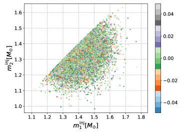
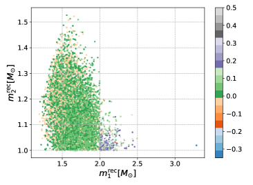
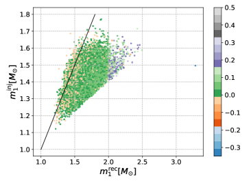
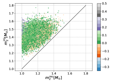
Figure 1: In this figure we compare the mass and spin recovery of one of the search pipelines, GstLAL (Messick et al., 2017), that meet the false alarm rate threshold of Eq.(2). Upper panel: This panel shows the $(m_{1},m_{2})$ pairs of a gaussian distributed BNS population $\sim\mathcal{N}[1.33M_{\odot},0.09M_{\odot}]$ (see Table 1). The left plot shows the masses injected following a normal distribution, as mentioned in Table 1, colored by the injected primary aligned spin component, $\chi_{1}^{z}$. The right plot shows the recovered masses colored by the recovered $\chi_{1}^{z}$. It can be seen that the distribution in the recovered space is significantly different from the one in the injected space. One may also see that the recovered spin values may be higher than the injected ones, especially in the case of higher mass ratio recoveries. Lower panel: This panel shows the injected values of the primary and secondary masses against their recovered values for low-mass injections. This is an example where one can see the systematic effect of the primary mass being recovered at higher values than the injected values. The secondary follows the opposite trend: the recovered value is lesser than the injected values. The effect also exists at higher mass ranges. Both plots are colored by the recovered $\chi_{1}^{z}$ values. Note the recovered $m_{1}^{\text{rec}}>2M_{\odot}$ (both panels) have higher values of recovered $\chi_{1}^{z}$. This is because the GstLAL search uses templates with low spins for masses $\leq 2M_{\odot}$ and high spins above that (see Fig. 1 $\&$ 2 in Mukherjee et al. (2018) for example). Even values slightly higher than $2M_{\odot}$ may result in high spin values compared to the injections.

LIGO/Virgo searches for transient GW signals fall into two broad categories: modeled compact binary coalescence (CBC) searches (Adams et al., 2016; Messick et al., 2017; Chu, 2017; Nitz et al., 2018; Abbott et al., 2019b) and un-modeled burst searches (Lynch et al., 2017; Klimenko et al., 2016). In this work, we are concerned with the former. The modeled searches use a discrete template bank of CBC waveforms to carry out matched filtering on the data. This is further broken down into realtime online analysis, and calibration corrected offline analysis. The online low-latency searches report CBC events in sub-minute latencies. They use waveform templates that are characterized by masses, $(m_{1},m_{2})$, and the dimensionless aligned/anti-aligned spins of the binary elements along the orbital angular momentum of the binary, $(\chi_{1}^{z},\chi_{2}^{z})$. They report a best matching template based on an appropriate detection statistic. We call the parameters of this template, $\{m_{1},m_{2},\chi_{1}^{z},\chi_{2}^{z}\}$, the point estimate. This data can be used for low-latency source property inference.

2.2 Capturing Detection Uncertainties

Since the source property inference is to be done based on the point estimates, the obvious pitfall in the inference is: How accurate are the point-estimates compared to the true parameters of the source? The primary goal of detection pipelines is to maximize detection efficiency at fixed false alarm probability. While some parameters like the chirp mass,

$$\mathcal{M}_{c}=(m_{1}m_{2})^{3/5}/(m_{1}+m_{2})^{1/5},$$ (1)

on which the signal strongly depends, are measured accurately, others like the individual mass or spin components are often inconsistent compared to the true parameters. Accurate parameter recovery is left to Bayesian parameter estimation analysis (Veitch et al., 2015; Ashton et al., 2019; Biwer et al., 2019).

Consider the case for the GstLAL search (Messick et al., 2017; Mukherjee et al., 2018; Sachdev et al., 2019) in Fig. 1. Here, we compare fake GW signals whose parameters we know a priori, to the recovered template i.e., point estimate, obtained from injecting the fake signals in detector noise and running the pipeline. Note that the recovered masses can sometimes be significantly different from the injected values, leading to an erroneous classification of the systems based on point-estimates alone. To alleviate this problem attempts were made to capture the uncertainty in the recovery of the parameters using an effective Fisher formalism (Cho et al., 2013). This method allows us to construct an ellipsoidal region of the parameter space around the point estimate that captures the uncertainty in the parameters under the Fisher approximation. This was used to create confidence regions in the parameter estimation code, RapidPE (Pankow et al., 2015) from which it was implemented in EM-Bright pipeline to construct $90\%$ confidence regions in three dimensions – chirp mass, symmetric mass ratio and effective spin. This ellipsoidal region was populated uniformly with one thousand points (besides the original triggered point). The fraction of these ellipsoid samples which had $m_{2}<m^{\text{NS}}_{\text{max}}$ constituted the $p(\texttt{HasNS})$ value, while the fraction that had non-vanishing disk mass, $M_{\text{disk}}>0$ from the Foucart (2012) fit, constituted $p(\texttt{HasRemnant})$ value.

3 Machine learning based classification

Table 1: The table lists the different population features used in the injection campaign. This includes signals in the three categories of CBC signals - binary black hole (BBH), neutron star black hole (NSBH) and binary neutron star (BNS) categories. The BBH category has both aligned and isotropic spin distributions. The BNS category has high spinning and low spinning systems to account for isolated high spinning neutron stars and galactic binaries. The NSBH category, includes $\delta$ function distributions along with uniform in log mass distribution. The $U,\mathcal{N},\delta$ imply uniform, normal and delta function distributions respectively. These injections densely sample possible populations of binaries. The number of found injections that passed the FAR threshold in Eq. (2) used in training are listed in the right-most column. The campaign uses the SpinTaylorT4 approximant for BNS injections, and effective one body calibrated to numerical relativity SEOBNR approximant for NSBH and BBH injections.

Type	Mass distribution	Spin distribution	Num. Injections
BBH	$U[\log m_{1},\log m_{2}]$	$|\chi^{\mathrm{max}}|=0.99$ (Isotropic)	$4.0\times 10^{4}$
BBH	$U[\log m_{1},\log m_{2}]$	$|\chi^{\mathrm{max}}|=0.99$ (Aligned)	$1.9\times 10^{4}$
BNS	$\mathcal{N}[1.33M_{\odot},0.09M_{\odot}]$	$|\chi^{\mathrm{max}}|=0.05$ (Isotropic)	$1.6\times 10^{4}$
BNS	$U[m_{1},m_{2}]$	$|\chi^{\mathrm{max}}|=0.40$ (Isotropic)	$1.6\times 10^{4}$
NSBH	$U[\log m_{1},\log m_{2}]$	$|\chi^{\mathrm{max}}_{\mathrm{NS}}|=0.40$; $|\chi^{\mathrm{max}}_{\mathrm{BH}}|=0.99$ (Aligned)	$1.9\times 10^{4}$
NSBH	$\delta(m_{1}-5M_{\odot},m_{2}-1.4M_{\odot})$	$|\chi^{\mathrm{max}}_{\mathrm{NS}}|=0.05$; $|\chi^{\mathrm{max}}_{\mathrm{BH}}|=0.99$ (Aligned/Isotropic)	$1.6\times 10^{4}$/$1.5\times 10^{4}$
NSBH	$\delta(m_{1}-10M_{\odot},m_{2}-1.4M_{\odot})$	$|\chi^{\mathrm{max}}_{\mathrm{NS}}|=0.05$; $|\chi^{\mathrm{max}}_{\mathrm{BH}}|=0.99$ (Aligned/Isotropic)	$1.7\times 10^{4}$/$1.3\times 10^{4}$
NSBH	$\delta(m_{1}-30M_{\odot},m_{2}-1.4M_{\odot})$	$|\chi^{\mathrm{max}}_{\mathrm{NS}}|=0.05$; $|\chi^{\mathrm{max}}_{\mathrm{BH}}|=0.99$ (Aligned/Isotropic)	$1.8\times 10^{4}$/$1.3\times 10^{4}$

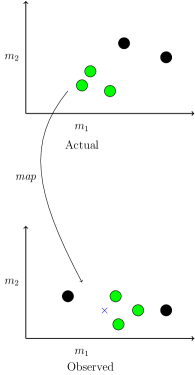
Figure 2: This figure is an qualitative illustration of the binary classification treatment of the problem. The top panel represent the true parameter space of binaries i.e, the injected parameters in this case, where the two colors represents satisfying either of the conditions in Eq. (3, 4). The lower panel is the parameter space of the recovery i.e., what the search reports. For the training process, the parameters in the recovered space are the features, while the label is inferred from the actual parameters. A fiducial detection during the production running is represented by the $\times$ mark in this plane. The probability of this fiducial detection being either of the two binary classes is determined from the nearest neighbors in the recovered parameter space.

The method of uncertainty ellipsoids handles the statistical uncertainties of the parameters from the low-latency search pipelines. However, the underlying Fisher approximation is only suitable in the case of high signal to noise ratio, when the parameter uncertainties are expected to be Gaussian distributed (see Sec. II of Cutler & Flanagan (1994) for example). Also, it is not robust in capturing any bias that a search might have. Such trends are seen, for example, in Fig. 1 where the $m_{1}$ parameter is recovered to be larger than the injected value, while the $m_{2}$ parameter is recovered to be smaller. Such uncertainties are more often the dominant source of error in this inference. While they decrease as the significance increases, they may be pronounced otherwise. Capturing and correcting such selection effects can be done by supervised machine learning algorithms. By injecting fake signals into real noise, performing the search, and comparing the recovered parameters with the original parameters of injections, one gets the map between the injected and recovered parameters. This is qualitatively illustrated in Fig. 2. Given a broad training set, the supervised algorithm learns this map. The training features are recovered parameters obtained after running the search, however, the labels of having a NS or remnant are determined from the injected values. It should be highlighted that we are not using machine learning to predict the recovered parameters from the injected values, or vice versa. Rather we use it for binary classification, correcting for selection biases that could have, otherwise, given an erroneous answer from the point estimate. We return the probability that the binary had a component less that $3M_{\odot}$, which we assume to be a conservative upper limit of the NS mass, and the probability that it had remnant matter based on the Foucart et al. (2018) (hereafter F18) expression.

3.1 Injection Campaign

In this study, we use a broad injection set that well samples the space of compact binaries. The distribution of the masses and spins is tabulated in Table 1. The injections are simulated waveforms placed in real detector noise at specific times. The BNS injections use the SpinTaylorT4 approximant (Buonanno et al., 2009), while NSBH and BBH injections use the SEOBNR approximant (Bohé et al., 2017). We consider the injections made in two detector operations from O2 (see Table 4 for times). The population contains uniform/log-uniform distribution of the masses, and both aligned and isotropic distributions of spins. It was used for the spacetime volume sensitivity analysis for the GstLAL search in Abbott et al. (2019b). In particular, injection campaigns were conducted for all astrophysical categories (BNS, NSBH, BBH) to analyze search sensitivity. We use the results, as a by product, to train our algorithm.

For an injection campaign, as this one, fake GW signals are put in real detector noise, followed by which the search is run, just as in the case of analyzing the production data. The injections maybe recovered based on the noise properties, and the GW intrinsic (masses and spins) and extrinsic (distance, sky location etc.) parameters. Since we are using real data, the dynamic variation of the power spectral density is taken into account (see Table 4 for the stretch of data used, and the splitting of the data into chunks). Not all injections are found by the searches, partly because of the signal strength, or from having them at a sky location where the detectors are not sensitive. The search reports triggers coincident signal across multiple detectors, simultaneously getting a high detection statistic. The triggers are assigned a false alarm rate (FAR) based on the frequency of background triggers that are assigned an equal or more significant value of the detection statistic. If the time of an injection coincides with the time of recovery of a trigger, the injection is considered found. For this study, we further subsample to the set where the FAR of the recovered triggers corresponding to found injections is less than one per month,

FAR $$\leq 1/1\text{ month}$$ (2)

$$= 3.85\times 10^{-7}\text{Hz}.$$

This leaves us with $\sim 2.0\times 10^{5}$ injections to train our supervised algorithm. The breakdown into different populations is shown in Table 1. This FAR threshold is reasonable since the LIGO/Virgo public alerts in the third observing run consider a false alarm rate threshold of one per two months further modified by a trials factor which consider the number of independent searches (see https://emfollow.docs.ligo.org/userguide/).

3.2 Training Features and Performance

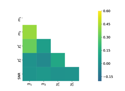
Figure 3: This is the correlation matrix of the recovered parameters that form our training set. The masses are expected to be correlated since there is a preference towards detecting heavier masses. The primary spin shows a strong correlation with the primary mass, however, the secondary spin recovery is not as correlated with the secondary mass. The signal-to-noise is mildly correlated with the remaining parameters. as expected since it is a detector frame parameter independent of the source properties.

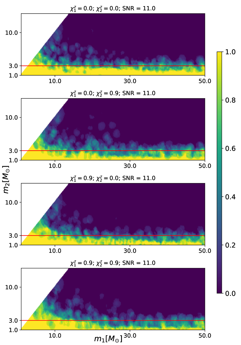
$p(\texttt{HasNS})$

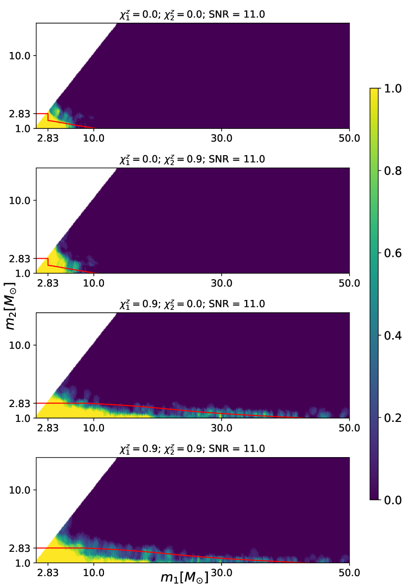
$p(\texttt{HasRemnant})$

Figure 4: This figure shows the predictions of the trained binary classifier upon performing a parameter sweep on the $(m_{1},m_{2})$ values. Note that each point on the plots is analogous to a point-estimate. We feed the trained classifier with arbitrary recovered parameter values and evaluate the predictions. Left panel: $p(\texttt{HasNS})$ predictions on the parameter space. We sweep over the masses, keeping the spin and SNR values fixed in each individual plot, incrementing the former as we move down. The horizontal line corresponds to $m_{2}=3M_{\odot}$ around which we expect a fuzzy region due to the detection uncertainties. Also, it is to be noted that the performance does not get affected by much upon increasing spin values since our original classification did not depend on it. Small changes are, however, expected due to correlation between the parameters during recovery (see Fig. 3). Right panel: $p(\texttt{HasRemnant})$ predictions on the parameter space. The region denoting non-zero remnant matter shows a more constrained classification about presence of matter compared to just having a NS in the binary. Also, note that unlike $p(\texttt{HasNS})$, $p(\texttt{HasRemnant})$ is strongly affected by the primary spin, as expected. The red curve in this panel represents the contour $M_{\text{rem}}(m_{1}^{\text{rec}},m_{2}^{\text{rec}},\chi_{1}^{z{\text{ rec}}})=0M_{\odot}$, calculated from recovered parameters using Eq.(4) of Foucart et al. (2018). Note that the $M_{\text{rem}}$ expression applies to NSBH systems and require a NS EoS which sets a maximum mass for the NS. In this study, we use the 2H EoS (Kyutoku et al., 2010) which has a maximum mass of $2.83M_{\odot}$. Mass components above this maximum mass are considered BHs which do not leave remnant matter upon coalescence. This explains the kink in the red curve in the top two panels.

Table 2: The table lists the percentage misclassification when using a threshold of $p(\text{HasNS}/\text{HasRemnant})=0.5$ to infer a binary to have a counterpart, as a function of the fraction of the dataset used for training and testing purposes. This could be thought as the scenario when an external partner has decided to follow-up CBCs that report $p(\text{HasNS})>0.5$ (or $p\text{HasRemnant}>0.5$). The table lists the fraction when such an observation would be a false positive. Out of the fraction of the total dataset used (left most column), we train using $90\%$ and test on the remaining $10\%$, cycling the training/testing set to have predictions on all points in the set. The uniform and inverse distance weighting of the nearest neighbors are used in all cases. We see that the answer starts to converge when using $\gtrsim 50\%$ of the total dataset. In light of verifying correlations (shown in Fig. 3) between parameters not affecting the prediction and the impurity, we trained using the Mahalanobis metric (Mahalanobis, 1936) in the parameter space mentioned in Eq.(5) . The misclassification does not change significantly based on the weighting scheme or the metric used.

Fraction	Misclassification $\%$ $p(\text{HasNS})$			Misclassification $\%$ $p(\text{HasRemnant})$
	Uniform	Inverse distance	Mahalanobis metric	Uniform	Inverse distance	Mahalanobis metric
$0.1$	$3.21$	$3.38$	$4.24$	$4.04$	$4.34$	$3.77$
$0.2$	$3.03$	$2.98$	$3.80$	$3.65$	$3.62$	$3.28$
$0.5$	$2.91$	$2.96$	$-$	$3.00$	$2.92$	$-$
$0.9$	$2.83$	$2.80$	$-$	$2.65$	$2.64$	$-$
$1.0$	$2.83$	$2.82$	$-$	$2.59$	$2.59$	$-$

For the HasNS quantity, to label an injection as having a NS, we use,

$$m_{2}^{\text{inj}}\leq 3M_{\odot}.$$ (3)

The value $\approx 3M_{\odot}$ has been regarded as a traditional and conservative upper limit for the NS maximum mass. The limit comes from the causality condition of the sound speed being less than the speed of light. The exact numbers, however, differ based on how the high core density is matched to the low crustal density, which is of the order of the nuclear density. If the low density is known to about twice the nuclear density, one obtains the $\approx 3M_{\odot}$ upper limit (see, for example, Rhoades & Ruffini, 1974; Kalogera & Baym, 1996; Lattimer, 2012). Observational evidences of pulsars obey this limit (see Table 1 of Lattimer, 2012). The total mass of the GW170817 system, $\approx 2.74M_{\odot}$, also provides an observational upper limit. Although the system could have undergone prompt collapse to form a BH, ejecting some mass prior to it (see Sec. 2.2 of Friedman (2018), and references therein for a discussion). Some GW template based searches, also, regard the $3M_{\odot}$ to be the upper boundary for placing BNS templates (Nitz et al., 2018). Thus, Eq. (3) is conservative and fundamental inference about the presence of a NS. However, we should mention that the presence of compact objects apart from BNS, NSBH, and BBH which satisfy Eq. (3) would be included in this inference. Our inference is only based on the secondary mass, and we do not prejudge the nature of the object.

For the HasRemnant quantity, to label an injection as having remnant matter, we use the F18 empirical fit to check for non-vanishing remnant matter (see Eq. (4) therein for expression),

$$M_{\text{rem}}(m_{1}^{\text{inj}},m_{2}^{\text{inj}},\chi_{1}^{z{\text{ inj}}})>0.$$ (4)

The F18 fit requires the compactness of the NS, and hence an EoS model. For this work, we use the 2H EoS (Kyutoku et al., 2010), which has a maximum NS mass of $2.83M_{\odot}$. Note that this value is not to be confused with the value mentioned in Eq.(3), which is the value considered for the HasNS categorization. The value $2.83M_{\odot}$ for HasRemnant comes from the usage of a particular model EoS. We use the condition in Eq. (4) only for the injections which have primary mass above the $2.83M_{\odot}$ and secondary mass below this value i.e., NSBH systems based on this EoS. The injections having both masses less than $2.83M_{\odot}$ are labeled as having remnant, while those with both masses above this value are labeled as not having remnant, based on the assumption that BNS mergers will always produce some remnant matter, while BBH mergers will will never do so. The 2H is an unusually stiff EoS resulting in NS radii $\sim 15-16$ km, but it errs towards larger values of the remnant matter, and therefore is a conservative choice in the sense of not misclassifying a CBC having remnant matter as otherwise, due to uncertainty in the EoS. This could be extended to compute disk masses based on different EoS models reported in the literature, giving each of them individual astrophysical weight and obtaining an EoS averaged disk mass, and thereby, a $p(\texttt{HasRemnant})$ after marginalizing over EoS.

We can restrict to the part of the parameter space on which the classification strongly depends on. We choose the following set as training features:

$$\boldsymbol{\beta}=\{m_{1},m_{2},\chi_{1}^{z},\chi_{2}^{z},{\rm SNR}\}\,.$$ (5)

The reason for using more parameters than those which are used to label the injections is because the recovered parameters have correlations (see Fig. 3). For example, the masses are expected to be positively correlated since the chirp mass is recovered fairly accurately and is an increasing function of the individual masses. There can also exist biases in the recovery due to degeneracies in the space of CBC GW signals. For example, high spin recovery is associated with high mass ratio. Regarding the choice of the feature set to be used, the masses and primary spins are natural since they are the intrinsic properties of the binary on which the source properties depend. As for a detection specific property, we use the signal to noise ratio, SNR, since it captures the general statistical uncertainty in the recovered parameters.

With this set, we use the machinery of supervised learning provided by the scikit-learn library (Pedregosa et al., 2011) to train a binary classifier based on the search results. Once trained, the classifier outputs a probability $p(\texttt{HasNS})$ or $p(\texttt{HasRemnant})$ given arbitrary but physical values of $\boldsymbol{\beta}$. We tested the performance using two non-parametric algorithms: KNeighborsClassifier and RandomForestClassifier, both provided in the scikit-learn library. We found that the former outperforms the latter in our case and is used for this study.  We train it using 11 neighbors – twice the number of dimensions plus one to break ties. The collection of parameters of a point-estimate is a point in this parameter space. To obtain the probability of this point having a secondary mass $\leq 3M_{\odot}$ or having some remnant matter based on F18 expression, we use the nearest neighbors from the training set, weighting them by the inverse of their distance from the fiducial point,

$$p(\texttt{HasNS/HasRemnant})=\frac{\sum_{\tiny{\texttt{HasNS/HasRemnant}}}w_{K}}{\sum w_{K}},$$ (6)

where the numerator (denominator) goes over neighbors that satisfy Eq.(3, 4) (all neighbors) of the fiducial point, and $w_{K}=1/d_{K}$ ($w_{K}=1$) for the inverse distance (uniform) weighting. We also used the Mahalanobis metric (Mahalanobis, 1936) in the space of $\boldsymbol{\beta}$ where distance, and therefore, nearest neighbors are determined via,

$$d_{K}=(\textbf{x}-\tilde{\textbf{x}})^{T}\Sigma^{-1}(\textbf{x}-\tilde{\textbf{x}}),$$ (7)

where $\tilde{\textbf{x}}$ is the mean and $\Sigma$ is the covariance matrix of the training set. This is done in the light of handling correlations. We, however, find that the metric or weighting scheme used does not affect the result significantly (see Table 2).

3.3 ROC Curve

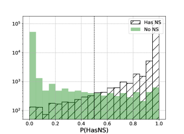
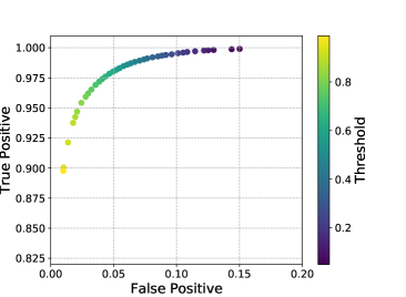
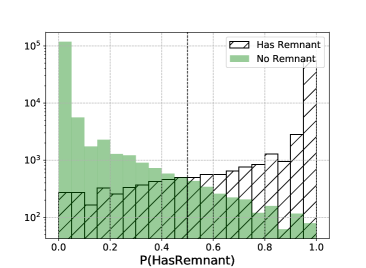
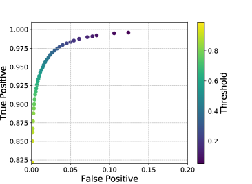
Figure 5: This figure shows the receiver operating characteristic curve for the classifier. It shows the true-positive against the false positive as a function of the threshold to classify binaries as having an NS or having remnant matter. Top panel: The left figure is a histogram of the $p(\text{HasNS})$ values for the injections which represented a binary that had an NS and for those does that did not. In the limit of perfect performance, the values for the former (latter) should be at $p(\text{HasNS})=1$ ($p(\text{HasNS})=0$). The true positive and false negative performance is decided based on the threshold that is applied to make the decision. For example, using the value of $p(\text{HasNS})=0.5$ (dot-dashed vertical line) would imply that all the values to the right of the line are decided as having a NS. While such a decision captures most of the true NS bearing binaries, one can notice a small misclassification fraction. The right figure shows the fractions as a function of this threshold. Bottom panel: Similar plots as the top panel except that the values correspond to the binary having remnant matter after merger.

Table 3: The table lists some example values of true positive and false positive numbers for changing values of the threshold used in Fig. 5. The column containing threshold values correspond to the colobar in both panels. The true positive and false positive values are to be read off based on HasNS/HasRemnant case.

Threshold	TP(HasNS)	FP(HasNS)	TP(HasRemnant)	FP(HasRemnant)
0.07	0.999	0.144	0.995	0.106
0.27	0.995	0.096	0.979	0.040
0.51	0.986	0.061	0.949	0.014
0.80	0.959	0.028	0.894	0.003
0.94	0.900	0.010	0.822	0.001

In the case of perfect performance, one expects the trained algorithm to predict $p(\texttt{HasNS})=1$ ($p(\texttt{HasRemnant})=1$) from the recovered parameters of the fake injections which originally had a NS (had remnant matter). On the other hand, in absence a NS component we also do not expect any remnant matter and hence expect $p(\texttt{HasNS}/\texttt{HasRemnant})=0$. In order to test the accuracy of the classifier we trained the algorithm on $90\%$ of the dataset and tested it on the remaining $10\%$, cycling the training/testing combination on the full dataset. The results are shown in Fig. 5. While most of the binaries are correctly classified as shown in the histogram plot (left panel) for the two quantities, there is a small fraction which does not end up getting perfect score ($p(\texttt{HasNS})=1$). The choice of threshold value to consider a binary suitable for follow-up operations would result in an impurity fraction. For example, if we use $p(\texttt{HasNS})\geq 0.5$, shown as a dashed vertical line in the upper left panel of Fig. 5, the contribution of the “No NS” histogram to the right of that line constitutes the false-positive. The variation of the efficiency with the false-positive as a function of the threshold applied is shown in right panels of Fig. 5. Some example values are listed in Table 3.3. The threshold could be set depending on the desired efficiency or, alternatively, the false positive to tolerate. We would like to highlight that the ROC curve depends on the relative rates of the different astrophysical sources. In this injection campaign each population has been densely sampled, without considering the relative rates. However, the current methodology works given an injection campaign curated based on astrophysical rate estimates of mergers as more observations are made.

The predictions of a parameter sweep on the $(m_{1},m_{2})$ values is shown in Fig. 5. Considering, the $p(\texttt{HasNS})$ plot, a perfect performance of the search would have rendered the region under the vertical line of $m_{2}=3M_{\odot}$ as $p(\texttt{HasNS})=1$. In reality, we expect a fuzz around the $m_{2}=3M_{\odot}$ line, as shown in the figure. The $p(\texttt{HasRemnant})$ is behaving as expected with respect to the increasing spin values, increasing the region having non-vanishing remnant mass boundary.

4 Conclusion

The low-latency inference about the presence of a neutron-star or post merger remnant matter in a compact binary merger provides crucial information about whether the binary will have an EM counterpart, and be worth following up for the observing partners. Such time sensitive inference has to be carried out from the low-latency point-estimate parameters provided by the gravitational wave realtime search pipelines. However, the point-estimate masses and spins could be off from the true estimate. Bayesian parameter estimation provides the best answer to such inference but it takes $\sim$ hours to $\sim$ days to complete. In order to correct for such systematics in low-latency, we show the use of supervised machine learning on the parameter recovery of the GstLAL online search pipeline from LIGO/Virgo operations. The result is a binary classifier that is trained based on an injection campaign to learn such systematics. Once trained, the real time computation on arbitrary binaries is sub-second. This method is adaptive to the change of template banks in the low-latency search algorithms provided the injection campaigns are conducted. Also, it is adaptive to the change in the noise power spectral density of the interferometer which naturally manifests in the performance of the search. While we have used a broad training set for the purposes of this paper, the methodology could be extended to incorporate astrophysical rates by curating injection campaigns based on our knowledge of the rates of binary mergers.

Appendix A Parameter sweep showing variation with SNR

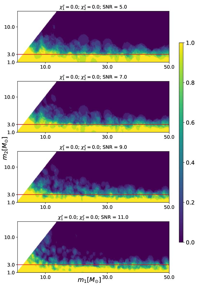
$p(\texttt{HasNS})$

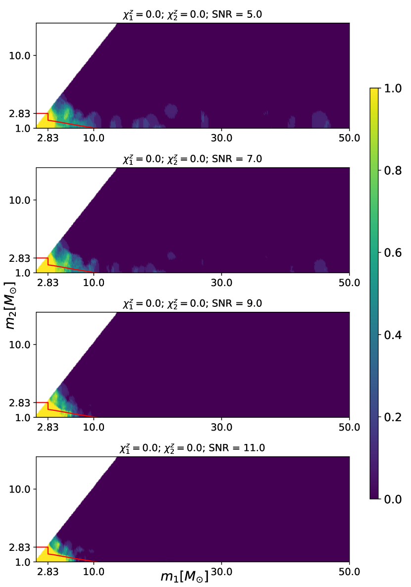
$p(\texttt{HasRemnant})$

Figure 6: This figure is an extension of Fig. 4. Here we see the behavior of the predictions from the binary classifiers as the signal to noise (SNR) of recovery increases. Left panel: Variation in $p(\texttt{HasNS})$ with SNR. Right panel: Variation in $p(\texttt{HasRemnant})$ with SNR.

In this section, we make in extension of the parameter sweep results shown in Fig. 4. Here we sweep over the $(m_{1},m_{2})$ values but keep the values of the spins fixed, only varying the signal-to-noise (SNR). The result is shown in Fig. 6. It is expected that the uncertainty in the recovered parameter should decrease with the increase in SNR which manifests as a decrease in the fuzzy region separating the bright ($p(\texttt{HasNS})=1$/$p(\texttt{HasRemnant})=1$) and dark ($p(\texttt{HasNS})=0$/$p(\texttt{HasRemnant})=0$) regions.

Appendix B GstLAL Injection sets

Table 4: The table contains the calender times for two detector (H1L1) chunks of LIGO O2 data. We consider the injections performed by the GstLAL search in these durations for this study. The timeseries is available in https://www.gw-openscience.org/data/

GstLAL chunk	Start date	End date
Chunk 02	Wed Nov 30 16:00:00 GMT 2016	Fri Dec 23 00:00:00 GMT 2016
Chunk 03	Wed Jan 04 00:00:00 GMT 2017	Sun Jan 22 08:00:00 GMT 2017
Chunk 04	Sun Jan 22 08:00:00 GMT 2017	Fri Feb 03 16:20:00 GMT 2017
Chunk 05	Fri Feb 03 16:20:00 GMT 2017	Sun Feb 12 15:30:00 GMT 2017
Chunk 06	Sun Feb 12 15:30:00 GMT 2017	Mon Feb 20 13:30:00 GMT 2017
Chunk 07	Mon Feb 20 13:30:00 GMT 2017	Tue Feb 28 16:30:00 GMT 2017
Chunk 08	Tue Feb 28 16:30:00 GMT 2017	Fri Mar 10 13:35:00 GMT 2017
Chunk 09	Fri Mar 10 13:35:00 GMT 2017	Sat Mar 18 20:00:00 GMT 2017
Chunk 10	Sat Mar 18 20:00:00 GMT 2017	Mon Mar 27 12:00:00 GMT 2017
Chunk 11	Mon Mar 27 12:00:00 GMT 2017	Tue Apr 04 16:00:00 GMT 2017
Chunk 12	Tue Apr 04 16:00:00 GMT 2017	Fri Apr 14 21:25:00 GMT 2017
Chunk 13	Fri Apr 14 21:25:00 GMT 2017	Sun Apr 23 04:00:00 GMT 2017
Chunk 14	Sun Apr 23 04:00:00 GMT 2017	Mon May 08 16:00:00 GMT 2017
Chunk 15	Fri May 26 06:00:00 GMT 2017	Sun Jun 18 18:30:00 GMT 2017
Chunk 16	Sun Jun 18 18:30:00 GMT 2017	Fri Jun 30 02:30:00 GMT 2017
Chunk 17	Fri Jun 30 02:30:00 GMT 2017	Sat Jul 15 00:00:00 GMT 2017
Chunk 18	Sat Jul 15 00:00:00 GMT 2017	Thu Jul 27 19:00:00 GMT 2017

In this section, we report the calender dates for the data chunks used in this study. These are tabulated in Table 4. The chunks cover most of the duration of the observing run, although they may not be contiguous corresponding to break in the observing run. Three detector injections were performed about the last $\sim 1$ month of the second observing run. Thus, their length and hence the missed found injections are smaller in number. As a future work, we plan to re-analyze the performance of the classifier based on injection campaigns in the third observing run as they are performed.

References

- Aasi et al. (2015) Aasi, J., et al. 2015, Classical and Quantum Gravity, 32, 074001
- Abbott et al. (2018) Abbott, B. P., Abbott, R., Abbott, T. D., Abernathy, M. R., et al. 2018, Living Reviews in Relativity, 21, 3
- Abbott et al. (2019a) Abbott, B. P., Abbott, R., Abbott, T. D., et al. 2019a, The Astrophysical Journal, 875, 161
- Abbott et al. (2017) Abbott, B. P., Abbott, R., Abbott, T. D., et al. 2017, ApJ Lett., 848, L12
- Abbott et al. (2019b) Abbott, B. P., Abbott, R., Abbott, T. D., et al. 2019b, Phys. Rev. X, 9, 031040
- Acernese et al. (2014) Acernese, F., et al. 2014, Classical and Quantum Gravity, 32, 024001
- Adams et al. (2016) Adams, T., Buskulic, D., Germain, V., et al. 2016, Classical and Quantum Gravity, 33, 175012
- Arcavi et al. (2017) Arcavi, I., Hosseinzadeh, G., Howell, D. A., et al. 2017, Nature, 551, 64
- Ashton et al. (2019) Ashton, G., Hübner, M., Lasky, P. D., et al. 2019, The Astrophysical Journal Supplement Series, 241, 27
- Barbieri et al. (2019) Barbieri, C., Salafia, O. S., Perego, A., Colpi, M., & Ghirlanda, G. 2019, Astronomy & Astrophysics, 625, A152
- Barnes & Kasen (2013) Barnes, J., & Kasen, D. 2013, The Astrophysical Journal, 775, 18
- Biwer et al. (2019) Biwer, C. M., Capano, C. D., De, S., et al. 2019, Publications of the Astronomical Society of the Pacific, 131, 024503
- Blandford & Znajek (1977) Blandford, R. D., & Znajek, R. L. 1977, Monthly Notices of the Royal Astronomical Society, 179, 433
- Bohé et al. (2017) Bohé, A., Shao, L., Taracchini, A., et al. 2017, Phys. Rev. D, 95, 044028
- Buonanno et al. (2009) Buonanno, A., Iyer, B. R., Ochsner, E., Pan, Y., & Sathyaprakash, B. S. 2009, Phys. Rev. D, 80, 084043
- Cho et al. (2013) Cho, H.-S., Ochsner, E., O’Shaughnessy, R., Kim, C., & Lee, C.-H. 2013, Phys. Rev. D, 87, 024004
- Chu (2017) Chu, Q. 2017, PhD thesis, The University of Western Australia
- Coulter et al. (2017) Coulter, D. A., Foley, R. J., Kilpatrick, C. D., et al. 2017, Science, 358, 1556
- Cutler & Flanagan (1994) Cutler, C., & Flanagan, E. E. 1994, Phys. Rev. D, 49, 2658
- Foucart (2012) Foucart, F. 2012, Phys. Rev. D, 86, 124007
- Foucart et al. (2018) Foucart, F., Hinderer, T., & Nissanke, S. 2018, Phys. Rev. D, 98, 081501
- Friedman (2018) Friedman, J. L. 2018, International Journal of Modern Physics D, 27, 1843018
- Graham et al. (2019) Graham, M. J., Kulkarni, S. R., Bellm, E. C., et al. 2019, Publications of the Astronomical Society of the Pacific, 131, 078001
- Hotokezaka & Nakar (2019) Hotokezaka, K., & Nakar, E. 2019, Radioactive heating rate of r-process elements and macronova light curve, , , arXiv:1909.02581
- Hunter (2007) Hunter, J. D. 2007, Computing In Science & Engineering, 9, 90
- Ivezić et al. (2008) Ivezić, Ž., Kahn, S. M., Tyson, J. A., et al. 2008, arXiv e-prints, arXiv:0805.2366
- Jones et al. (2001–) Jones, E., Oliphant, T., Peterson, P., et al. 2001–, SciPy: Open source scientific tools for Python, , , [Online; accessed ¡today¿]
- Kalogera & Baym (1996) Kalogera, V., & Baym, G. 1996, The Astrophysical Journal, 470, L61
- Kasen et al. (2015) Kasen, D., Fernández, R., & Metzger, B. D. 2015, Monthly Notices of the Royal Astronomical Society, 450, 1777
- Kasliwal et al. (2017) Kasliwal, M. M., Nakar, E., Singer, L. P., et al. 2017, Science, 358, 1559
- Klimenko et al. (2016) Klimenko, S., Vedovato, G., Drago, M., et al. 2016, Phys. Rev. D, 93, 042004
- Korobkin et al. (2012) Korobkin, O., Rosswog, S., Arcones, A., & Winteler, C. 2012, Monthly Notices of the Royal Astronomical Society, 426, 1940
- Kulkarni (2016) Kulkarni, S. R. 2016, in American Astronomical Society Meeting Abstracts, Vol. 227, American Astronomical Society Meeting Abstracts #227, 314.01
- Kyutoku et al. (2010) Kyutoku, K., Shibata, M., & Taniguchi, K. 2010, Phys. Rev. D, 82, 044049
- Lattimer (2012) Lattimer, J. M. 2012, Annual Review of Nuclear and Particle Science, 62, 485–515
- Lattimer & Schramm (1974) Lattimer, J. M., & Schramm, D. N. 1974, ApJ, 192, L145
- Li & Paczyński (1998) Li, L.-X., & Paczyński, B. 1998, The Astrophysical Journal, 507, L59
- Lipunov et al. (2017) Lipunov, V. M., Gorbovskoy, E., Kornilov, V. G., et al. 2017, The Astrophysical Journal, 850, L1
- Lynch et al. (2017) Lynch, R., Vitale, S., Essick, R., Katsavounidis, E., & Robinet, F. 2017, Phys. Rev. D, 95, 104046
- Mahalanobis (1936) Mahalanobis, P. C. 1936, Proceedings of the National Institute of Science of India, 12, 49
- McKinney (2010) McKinney, W. 2010, in Proceedings of the 9th Python in Science Conference, ed. S. van der Walt & J. Millman, 51 – 56
- Messick et al. (2017) Messick, C., Blackburn, K., Brady, P., et al. 2017, Phys. Rev. D, 95, 042001
- Mukherjee et al. (2018) Mukherjee, D., Caudill, S., Magee, R., et al. 2018, arXiv e-prints, arXiv:1812.05121
- Nitz et al. (2018) Nitz, A. H., Dal Canton, T., Davis, D., & Reyes, S. 2018, Phys. Rev. D, 98, 024050
- Pankow et al. (2015) Pankow, C., Brady, P., Ochsner, E., & O’Shaughnessy, R. 2015, Phys. Rev. D, 92, 023002
- Pannarale & Ohme (2014) Pannarale, F., & Ohme, F. 2014, The Astrophysical Journal, 791, L7
- Pedregosa et al. (2011) Pedregosa, F., Varoquaux, G., Gramfort, A., et al. 2011, Journal of Machine Learning Research, 12, 2825
- Rhoades & Ruffini (1974) Rhoades, C. E., & Ruffini, R. 1974, Phys. Rev. Lett., 32, 324
- Ruiz & Shapiro (2017) Ruiz, M., & Shapiro, S. L. 2017, Physical Review D, 96, doi:10.1103/physrevd.96.084063
- Sachdev et al. (2019) Sachdev, S., Caudill, S., Fong, H., et al. 2019, arXiv e-prints, arXiv:1901.08580
- Shibata & Hotokezaka (2019) Shibata, M., & Hotokezaka, K. 2019, Annual Review of Nuclear and Particle Science, 69, null
- Singer & Price (2016) Singer, L. P., & Price, L. R. 2016, Phys. Rev. D, 93, 024013
- Singer et al. (2016) Singer, L. P., Chen, H.-Y., Holz, D. E., et al. 2016, The Astrophysical Journal Letters, 829, L15
- Soares-Santos et al. (2017) Soares-Santos, M., Holz, D. E., Annis, J., et al. 2017, The Astrophysical Journal, 848, L16
- Tanaka & Hotokezaka (2013) Tanaka, M., & Hotokezaka, K. 2013, The Astrophysical Journal, 775, 113
- Tanvir et al. (2017) Tanvir, N. R., Levan, A. J., González-Fernández, C., et al. 2017, The Astrophysical Journal, 848, L27
- van der Walt et al. (2011) van der Walt, S., Colbert, S. C., & Varoquaux, G. 2011, Computing in Science Engineering, 13, 22
- Veitch et al. (2015) Veitch, J., Raymond, V., Farr, B., et al. 2015, Phys. Rev. D, 91, 042003