Representation theory and products of random matrices in $\text{SL}(2,{\mathbb{R}})$

Abstract.

The statistical behaviour of a product of independent, identically distributed random matrices in $\text{SL}(2,{\mathbb{R}})$ is encoded in the generalised Lyapunov exponent $\Lambda$; this is a function whose value at the complex number $2\ell$ is the logarithm of the largest eigenvalue of the transfer operator obtained when one averages, over $g\in\text{SL}(2,{\mathbb{R}})$, a certain representation $T_{\ell}(g)$ associated with the product. We study some products that arise from models of one-dimensional disordered systems. These models have the property that the inverse of the transfer operator takes the form of a second-order difference or differential operator. We show how the ideas expounded by N. Ja. Vilenkin in his book [Special Functions and the Theory of Group Representations, American Mathematical Society, 1968.] can be used to study the generalised Lyapunov exponent. In particular, we derive explicit formulae for the almost-sure growth and for the variance of the corresponding products.

1. Introduction

In his remarkable paper [16], Furstenberg succeeded in generalising the law of large numbers to products

$$\Pi_{n}:=g_{n}\cdots g_{2}g_{1}$$

of independent, identically-distributed random elements of a matrix group $G$. In his theory, an important part is played by a compact homogeneous space, now known as the Furstenberg boundary, on which the group acts, and the problem of determining the growth rate of the product is reduced to that of finding a certain measure on this boundary that is invariant under the action of elements drawn at random from the group. The growth rate is called the Lyapunov exponent of the product, and the problem of computing it— or the invariant measure— given a probability measure on the group, is notoriously difficult.

By elaborating ideas that go back to the seminal works of Dyson [12], Schmidt [35], Frisch & Lloyd [15], Halperin [21], Kotani [24] and Nieuwenhuizen [31], we have, over the past few years, found several instances of products of random matrices in $\text{SL}(2,{\mathbb{R}})$ for which the growth rate can be obtained explicitly in terms of special functions such as the hypergeometric, Bessel, confluent hypergeometric functions and so on; see the survey [7]. There are also a few cases involving larger matrix groups where calculations have been possible; two such cases were found by Newman [30] and Forrester [14], who succeeded in obtaining formulae for all the Lyapunov exponents of certain products in terms of the gamma and dilogarithmic functions; the key observation, in these particular cases, is that the invariant measure coincides with the rotation-invariant measure.

Now, since Vilenkin’s classic book [41], it is widely appreciated that there is a close relationship between special functions and the theory of group representation. It is the purpose of the present paper to explain how Vilenkin’s ideas may be brought to bear on this problem. To the best of our knowledge, this is, in itself, an original contribution to the literature on products of random matrices; it has the merit of providing a unified presentation of the ideas originating from the work of Frisch & Lloyd, with the practical benefit that calculations can be pushed further, using concepts of such generality that one may also envisage applications to other groups. There is some overlap with the approach and the results that will appear in a forthcoming publication by one of us [38], but here, although we shall not assume any prior knowledge of the subject, the emphasis is on the connections with representation theory.

The focus of our analysis is the generalised Lyapunov exponent, which will be defined in the next paragraph. This is an important mathematical object, relevant in several physical contexts: chaotic dynamics and multifractal analysis [8]; fluid dynamics [40]; classical dynamics of an oscillator driven by parametric noise [36, 45]; polymers in a random landscape [17]. In particular, the generalised Lyapunov exponent yields information on the fluctuations of products of random matrices; these fluctuations are of interest in relation with Anderson localisation [10, 11, 34, 37] and also in relation with disordered Ising spin chains [5].

In the remainder of this extensive introduction, we provide a summary of those facts that we shall need in order to develop our material. We then describe the content of the paper in broad terms, state our main results, and provide some indication of how these results relate to the work of others— postponing the technical details to the remaining sections. We shall deal exclusively with the case where

$$G:=\text{SL}(2,{\mathbb{R}})$$

and then comment at the end of the paper on the possibility of extending our ideas to other semi-simple groups.

1.1. The generalised Lyapunov exponent and Tutubalin’s transfer operator

Inspired by the work of Furstenberg, Tutubalin [39] proved a central limit theorem for products of random matrices; he showed that, as $n\rightarrow\infty$,

$$\frac{\ln\left|{\mathbf{x}}\Pi_{n}\right|-n\gamma}{\sigma\sqrt{n}}$$

converges in distribution to a normal random variable. Here

(1.1) $$\gamma:=\lim_{n\rightarrow\infty}\frac{1}{n}\,{\mathbb{E}}\left(\ln\left|{\mathbf{x}}\Pi_{n}\right|\right)$$

and

(1.2) $$\sigma^{2}:=\lim_{n\rightarrow\infty}\frac{1}{n}\,{\mathbb{E}}\left(\ln^{2}\left|{\mathbf{x}}\Pi_{n}\right|-n^{2}\gamma^{2}\right)$$

where ${\mathbf{x}}$ is an arbitrary non-zero vector, $|\cdot|$ is an arbitrary norm on the vector space, and the expectation is taken with respect to the probability measure on the group. It is a fact that the limits do not depend on the precise choice of ${\mathbf{x}}$ and $|\cdot|$.

Both $\gamma$ and $\sigma^{2}$ may be expressed in terms of the generalised Lyapunov exponent of the product, defined by

$$\Lambda({2\ell}):=\lim_{n\rightarrow\infty}\frac{\ln{\mathbb{E}}\left(\left|\Pi_{n}^{t}\Pi_{n}\right|^{\ell}\right)}{n}$$

where $g^{t}$ denotes the transpose of $g$. Here, we have chosen to write the argument of $\Lambda$ in this unusual way to indicate its relationship with the index $\ell$ used by Vilenkin [41] and Vilenkin & Klimyk [42] to label a certain family of representations of the group $\text{SL}(2,{\mathbb{R}})$. The existence of the limit in this definition is a non-trivial matter but, in case of existence, it is again a fact that the limit on the right-hand side does not depend on the choice of norm. It is also clear from the definition that the generalised Lyapunov exponent is unchanged if we replace the $g_{n}$ in the product by $g_{n}^{t}$. Other equivalent definitions are used in the literature:

(1.3) $$\Lambda({2\ell})=\lim_{n\rightarrow\infty}\frac{\ln{\mathbb{E}}\left(\left|\Pi_{n}{\mathbf{x}}\right|^{2\ell}\right)}{n}=\lim_{n\rightarrow\infty}\frac{\ln{\mathbb{E}}\left(\left|{\mathbf{x}}\Pi_{n}\right|^{2\ell}\right)}{n}\,.$$

The last of these formulae yields

(1.4) $$\gamma=\Lambda^{\prime}(0)\;\;\text{and}\;\;\sigma^{2}=\Lambda^{\prime\prime}(0)\,.$$

Tutubalin proved his theorem by expressing the generalised Lyapunov exponent as the largest eigenvalue of a certain operator. To describe his approach, we begin by remarking that every matrix

$$g=\begin{pmatrix}a&b\\ c&d\end{pmatrix}\in G$$

acts on ${\mathbb{R}}_{\ast}^{2}:={\mathbb{R}}^{2}\backslash\{{\mathbf{0}}\}$ from the right according to

$${\mathbf{x}}\cdot g:=\begin{pmatrix}x_{1}&x_{2}\end{pmatrix}\begin{pmatrix}a&b\\ c&d\end{pmatrix}=\begin{pmatrix}ax_{1}+cx_{2}&bx_{1}+dx_{2}\end{pmatrix}\,.$$

To every $g\in G$, we assign a linear map, denoted $T(g)$, defined on the space $V$ of all functions $v:\,{\mathbb{R}}_{\ast}^{2}\rightarrow{\mathbb{C}}$ by

(1.5) $$\left[T(g)v\right]({\mathbf{x}}):=v({\mathbf{x}}\cdot g)=v\left(ax_{1}+cx_{2},bx_{1}+dx_{2}\right)\,.$$

The map $g\mapsto T(g)$ obtained in this way is a representation of the group — namely, it satisfies the following properties: Firstly, if $e$ denotes the identity matrix then $T(e)$ is the identity operator; secondly,

$$\forall\,g_{1},\,g_{2}\in G\,,\;\;T(g_{1}g_{2})=T({g_{1}})\,T({g_{2}})\,.$$

The vector space $V$, on which the operators $T(g)$ are defined, is called the representation space.

We introduce the function $1_{\ell}\in V$ defined by

(1.6) $$1_{\ell}({\mathbf{x}})=|{\mathbf{x}}|^{2\ell}\,.$$

For every ${\mathbf{x}}\in{\mathbb{R}}_{\ast}^{2}$ and every $g\in G$, we may write

$$\left[T(g){1}_{\ell}\right]({\mathbf{x}})={1}_{\ell}\left({\mathbf{x}}\cdot g\right)=\left|{\mathbf{x}}g\right|^{2\ell}\,.$$

Hence

$$\left|{\mathbf{x}}\Pi_{n}\right|^{2\ell}=\left[T\left({\Pi_{n}}\right){1}_{\ell}\right]({\mathbf{x}})\,.$$

By using the fact that the $g_{n}$ are independent with the same distribution, we deduce

(1.7) $${\mathbb{E}}\left(\left|{\mathbf{x}}\Pi_{n}\right|^{2\ell}\right)=\left[{\mathscr{T}}^{n}{1}_{\ell}\right]({\mathbf{x}})$$

where

(1.8) $${\mathscr{T}}:={\mathbb{E}}\left[T(g)\right]\,.$$

In the literature, the operator ${\mathscr{T}}$ is often called the transfer operator associated with the product of random matrices [2, 32]. Heuristically, if this operator admits an eigenvalue of largest modulus, then the generalised Lyapunov exponent will be obtained by taking its logarithm.

In his paper, Tutubalin proved that this heuristic argument is indeed correct if one assumes that the matrices are drawn from a probability distribution that has a density with respect to the Haar measure on the group $G$. This hypothesis has since been weakened considerably; see [2, 3] and the references therein. Important and relevant as this question is, we shall not be concerned with stating or proving general theorems that guarantee the existence of an eigenvalue of the transfer operator of largest modulus. Rather, our aim in this paper is to bring out the practical usefulness of representation theory by considering specific probability measures on the group for which the heuristic argument leads to explicit calculations of $\gamma$ and $\sigma^{2}$.

1.2. Reducibility, equivalence and unitarity of representations

The analysis of the spectral problem obviously entails the search for vector spaces invariant under the action of the transfer operator.

Definition 1.1.

We say that a subspace of $V$ is invariant under a representation $T$ if, for every $g\in G$, $T(g)$ maps the subspace to itself. $T$ is called reducible if its representation space $V$ contains a proper invariant subspace. Otherwise, it is called irreducible.

Every subspace invariant for the representation is also invariant for the transfer operator. Now, the particular representation defined by Equation (1.5) is reducible, as the following makes clear.

Definition 1.2.

We say that $v$ is even (respectively odd) if

$$\forall\,{\mathbf{x}}\in{\mathbb{R}}_{\ast}^{2},\;\;v(-{\mathbf{x}})=v({\mathbf{x}})\;\;\text{(respectively $-v({\mathbf{x}})$)}\,.$$

For $\ell\in{\mathbb{C}}$, we say that $v$ is homogeneous of degree $2\ell$ if

$$\forall\,\tau>0\,,\;\forall\,{\mathbf{x}}\in{\mathbb{R}}_{\ast}^{2},\;\;v(\tau{\mathbf{x}})=\tau^{2\ell}v({\mathbf{x}})\,.$$

It is readily verified that the subspace consisting of all smooth even homogeneous functions of degree $2\ell$— which we shall denote by $V_{\ell}$— is invariant for $T$; the restrictions of $T$ and ${\mathscr{T}}$ to $V_{\ell}$ will be denoted by $T_{\ell}$ and ${\mathscr{T}}_{\ell}$ respectively. Another invariant subspace of $V$ is that consisting of all smooth odd homogeneous functions of degree $2\ell$; we shall not need to consider this invariant subspace because the function ${1}_{\ell}$ introduced earlier and defined by Equation (1.6) happens to be even.

Although the functions in the space $V_{\ell}$ are defined on the punctured plane, the requirement of homogeneity and evenness implies that they are completely characterised by the values they take on certain curves. These curves may be understood as parametrisations of the Furstenberg boundary, and there is some flexibility in choosing them; this will prove convenient when we consider specific probability measures on the group. The important point is that, although we may work with different curves, it is essentially always the same representation that is involved.

Definition 1.3.

Two representations $\widetilde{T}$ and $T$ with respective representation spaces $V$ and $\widetilde{V}$ are called equivalent if there exists an invertible map, say $Q:\,V\rightarrow\widetilde{V}$, such that

$$\widetilde{T}\,Q=Q\,T\,.$$

We then say that $\widetilde{T}$ and $T$ are realisations, in the spaces $\widetilde{V}$ and $V$ respectively, of the same representation.

Finally, in discussing the spectral problem for the transfer operator, we need to consider also the spectral problem for its adjoint, and this raises the technical question of finding an appropriate inner product for the space $V_{\ell}$.

Definition 1.4.

The representation $T_{\ell}$ is called unitary if $V_{\ell}$ is equipped with an inner product, say $\mathinner{\langle{\cdot|\cdot}\rangle}$, such that

$$\forall\,g\in G,\;\forall\,f,\,v\in V_{\ell},\,\;\;\mathinner{\langle{T_{\ell}(g)f|T_{\ell}(g)v}\rangle}=\mathinner{\langle{f|v}\rangle}\,.$$

We remark however that, even if an inner product can be found that makes $T_{\ell}$ unitary, this property is lost upon averaging over the group, and so will play only a very minor part in what follows.

Starting with Bargmann [1], the family of representations $T_{\ell}$ has been thoroughly studied [18, 41, 42]. We summarise in the following theorem those properties that will be relevant to our purpose:

Theorem 1.

The representation $T_{\ell}$ is reducible if and only if $\ell\in{\mathbb{Z}}$. In the reducible case, it may be decomposed into three irreducible subrepresentations: one, denoted $T_{\ell}^{0}$, in a space of finite dimension, and two others, denoted $T_{\ell}^{+}$ and $T_{\ell}^{-}$ and called “holomorphic”, in spaces of infinite dimension.

For $\ell\in{\mathbb{Z}}$ and $\varepsilon\in\{-,0,+\}$ (respectively $\ell\notin{\mathbb{Z}}$), the representations $T_{\ell}^{\varepsilon}$ and $T_{-\ell-1}^{\varepsilon}$ (respectively $T_{\ell}$ and $T_{-\ell-1}$) are equivalent.

Of the finite-dimensional representations, only $T_{0}^{0}$ is unitary, as it corresponds to the trivial representation in a one-dimensional space. The holomorphic subrepresentations are unitary with respect to a certain inner product and belong to the so-called discrete series. The only other values of $\ell$ for which $T_{\ell}$ can be made unitary are

$$\ell=-\frac{1}{2}+\text{\rm i}t\,,\;\;t\in{\mathbb{R}}\;\;\text{and}\;\;\ell\in(-2,-1)\cup(0,1)\,.$$

They are associated with the principal and the supplementary series respectively.

1.3. The one-parameter subgroups of $\text{SL}(2,{\mathbb{R}})$

The proof of Theorem 1 uses the so-called “infinitesimal method” which tackles questions of irreducibility, equivalence and unitarity by making systematic use of the infinitesimal generators associated with the one-parameter subgroups of $\text{SL}(2,{\mathbb{R}})$. These subgroups may be classified in terms of three types:

1. Elliptic

   $$k(t):=\begin{pmatrix}\cos\frac{t}{2}&-\sin\frac{t}{2}\\ \sin\frac{t}{2}&\cos\frac{t}{2}\end{pmatrix}\,.$$

2. Hyperbolic

   $$a_{1}(t):=\begin{pmatrix}\text{e}^{\frac{t}{2}}&0\\ 0&\text{e}^{-\frac{t}{2}}\end{pmatrix}\;\;\text{and}\;\;a_{2}(t):=\begin{pmatrix}\text{ch}\frac{t}{2}&\text{sh}\frac{t}{2}\\ \text{sh}\frac{t}{2}&\text{ch}\frac{t}{2}\end{pmatrix}\,.$$

3. Parabolic

   $$n_{+}(t):=\begin{pmatrix}1&t\\ 0&1\end{pmatrix}\;\;\text{and}\;\;n_{-}(t):=\begin{pmatrix}1&0\\ t&1\end{pmatrix}\,.$$

By definition, the generator associated with the one-parameter subgroup ${\mathbb{R}}\ni t\mapsto g(t)\in G$ is the operator on $V_{\ell}$ that maps $v$ to

$$\frac{d}{dt}\left\{T_{\ell}\left[g(t)\right]v\right\}\Bigl{|}_{t=0}\,.$$

A list of the infinitesimal generators for various realisations of $T_{\ell}$ may be found in Tables 1 to 4. We shall consider probability measures that lead to an explicit formula for ${\mathscr{T}}_{\ell}$ in terms of these infinitesimal generators. The fact that these generators are affine functions of the index $\ell$ will be important in what follows.

The subgroup $K$ occupies a special place in the harmonic analysis of $G$ as the largest compact subgroup, and there is a countable basis of $V_{\ell}$ consisting of eigenvectors of the corresponding infinitesimal generator. We shall denote these basis functions ${\mathbf{e}}_{\ell,n}$, $n\in{\mathbb{Z}}$, regardless of the particular realisation of the representation $T_{\ell}$. We draw attention to the important fact that the function $1_{\ell}$, defined by Equation (1.6), is a multiple of ${\mathbf{e}}_{\ell,0}$.

In order to work out how each generator acts on the basis functions, it is helpful to introduce a basis of the Lie algebra consisting of the operators

(1.9) $${J}_{0}:=\text{i}{K}\,,\;\;{J}_{\pm}:={A}_{1}\pm\text{i}{A}_{2}\,.$$

For instance, we have

(1.10) $${N}_{\pm}=\text{i}\left[\frac{{J}_{-}-{J}_{+}}{2}\pm{J}_{0}\right]\,.$$

The action of $N_{\pm}$ is then easily deduced from the identities

(1.11) $${J}_{0}\,{{\mathbf{e}}_{\ell,n}}=n\,{{\mathbf{e}}_{\ell,n}}$$

and

(1.12) $${J}_{+}\,{{\mathbf{e}}_{\ell,n}}=(\ell-n)\,{{\mathbf{e}}_{\ell,n+1}}\;\;\text{and}\;\;{J}_{-}\,{{\mathbf{e}}_{\ell,n}}=(\ell+n)\,{{\mathbf{e}}_{\ell,n-1}}\,.$$

In particular, the Casimir operator associated with the representation is defined by

$${C}:=A_{1}^{2}+A_{2}^{2}-K^{2}={J}_{0}^{2}+{J}_{0}+{J}_{-}{J}_{+}\,.$$

This operator commutes with the representation, and it is readily verified that it is a multiple of the identity operator ${I}$:

$${C}=\ell(\ell+1)\,{I}\,.$$

	Plane	Circle	Line	Hyperbola
${K}$	$\frac{x_{2}}{2}\frac{\partial}{\partial x_{1}}-\frac{x_{1}}{2}\frac{\partial}{\partial x_{2}}$	$-\frac{d}{d\theta}$	$-\ell x+\frac{1+x^{2}}{2}\frac{d}{dx}$	$\frac{\ell}{2}(\frac{1}{x}-x)+\frac{1+x^{2}}{2}\frac{d}{dx}$
${A}_{1}$	$\frac{x_{1}}{2}\frac{\partial}{\partial x_{1}}-\frac{x_{2}}{2}\frac{\partial}{\partial x_{2}}$	$\ell\cos\theta-\sin\theta\frac{d}{d\theta}$	$-\ell+x\frac{d}{dx}$	$x\frac{d}{dx}$
${A}_{2}$	$\frac{x_{2}}{2}\frac{\partial}{\partial x_{1}}+\frac{x_{1}}{2}\frac{\partial}{\partial x_{2}}$	$\ell\sin\theta+\cos\theta\frac{d}{d\theta}$	$\ell x+\frac{1-x^{2}}{2}\frac{d}{dx}$	$\frac{\ell}{2}(\frac{1}{x}+x)+\frac{1-x^{2}}{2}\frac{d}{dx}$
${N}_{+}$	$x_{1}\frac{\partial}{\partial x_{2}}$	$\ell\sin\theta+(\cos\theta+1)\frac{d}{d\theta}$	$2\ell x-x^{2}\frac{d}{dx}$	$\ell x-x^{2}\frac{d}{dx}$
${N}_{-}$	$x_{2}\frac{\partial}{\partial x_{1}}$	$\ell\sin\theta+(\cos\theta-1)\frac{d}{d\theta}$	$\frac{d}{dx}$	$\frac{\ell}{x}+\frac{d}{dx}$

Table 1. Infinitesimal generators associated with the representation $T_{\ell}$ for various one-parameter subgroups. The columns correspond to equivalent realisations of the representation in spaces of functions on the punctured plane, the circle, the line and the hyperbola respectively.

1.4. One-dimensional disordered systems

The class of probability measures for which the transfer operator has a simple expression in terms of generators arises naturally in connection with the one-dimensional disordered systems that were studied by Dyson [12] and Frisch & Lloyd [15]. So we provide a brief description of these models. The reader interested in their physical relevance will find further details in [7, 38].

Consider the differential equation

$$-\psi^{\prime\prime}+U\psi=\omega^{2}M^{\prime}\psi\,,\quad x>0\,.$$

Here, $U$ denotes the generalised function

$$U(x)=\sum_{j}u_{j}\,\delta(x-x_{j})$$

where the $x_{j}$ are the values taken by a Poisson process of intensity $\rho$, so that the jumps

$$l_{j}:=x_{j+1}-x_{j}>0$$

are independent and exponentially distributed with mean $1/\rho$. If we put $M^{\prime}(x)\equiv 1$ and draw the $u_{j}$ independently from some probability distribution, we obtain a model for the energy levels $\omega^{2}$ of a particle subject to a one-dimensional potential with impurities [15]. By introducing the derivative $\psi^{\prime}$ as an additional unknown, we can write this second-order differential equation as a first-order system. For $\omega^{2}=1$, the solution of the corresponding Cauchy problem may be expressed as a product $\Pi_{n}$ with elements of the form

$$g_{j}=\underbrace{\begin{pmatrix}\cos l_{j}&-\sin l_{j}\\ \sin l_{j}&\cos l_{j}\end{pmatrix}}_{k(2l_{j})\in K}\underbrace{\begin{pmatrix}1&u_{j}\\ 0&1\end{pmatrix}}_{n_{+}(u_{j})\in N_{+}}\,.$$

The analysis carried out by Frisch & Lloyd [15] and, later, Kotani [24], focused on the random process associated with the “Riccati variable” $\psi^{\prime}/\psi$.

By setting $U\equiv 0$ and

$$M^{\prime}(x)=\sum_{j}m_{j}\,\delta(x-x_{j})$$

we obtain instead a model for a (discrete) vibrating string, where $m_{j}$ is the punctual mass at $x_{j}$ and $\omega$ is now interpreted as a characteristic frequency. The solution of the Cauchy problem in the case $\omega=1$ is then a product of matrices of the form

$$g_{j}=\underbrace{\begin{pmatrix}1&0\\ l_{j}&1\end{pmatrix}}_{n_{-}(l_{j})\in N_{-}}\underbrace{\begin{pmatrix}1&-m_{j}\\ 0&1\end{pmatrix}}_{n_{+}(-m_{j})\in N_{+}}\,.$$

Dyson [12] considered the case where the $l_{j}$ and $m_{j}$ are drawn from gamma distributions. We alert the reader to the fact that our notation differs from Dyson’s; his string equation is

$$K_{j}\left(x_{j+1}-x_{j}\right)+K_{j-1}\left(x_{j-1}-x_{j}\right)=-m_{j}\omega^{2}x_{j}$$

where the $x_{j}$ are the positions of particles coupled together by springs that obey Hooke’s law, and $K_{j}$ is the elastic modulus of the spring between the $j$th and $(j+1)$th particles. The correspondence between this and our own equation is

$$x_{j}\sim\psi(x_{j})\;\;\text{and}\;\;K_{j}\sim 1/l_{j}\,.$$

Other models of a similar kind have been considered more recently in which $M^{\prime}\equiv 1$ and the potential function $U$ is “supersymmetric” [6]:

$$U=\frac{w^{\prime}}{2}+\frac{w^{2}}{4}\,,\;\;w(x):=\sum_{j}w_{j}\,\delta(x-x_{j})\,.$$

These models lead to products of matrices of the form

$$g_{j}=\underbrace{\begin{pmatrix}\cos l_{j}&-\sin l_{j}\\ \sin l_{j}&\cos l_{j}\end{pmatrix}}_{k(2l_{j})\in K}\underbrace{\begin{pmatrix}e^{\frac{w_{j}}{2}}&0\\ 0&e^{-\frac{w_{j}}{2}}\end{pmatrix}}_{a_{1}(w_{j})\in A_{1}}$$

or

$$g_{j}=\underbrace{\begin{pmatrix}\text{ch}\,l_{j}&\text{sh}\,l_{j}\\ \text{sh}\,l_{j}&\text{ch}\,l_{j}\end{pmatrix}}_{a_{2}(2l_{j})\in A_{2}}\underbrace{\begin{pmatrix}e^{\frac{w_{j}}{2}}&0\\ 0&e^{-\frac{w_{j}}{2}}\end{pmatrix}}_{a_{1}(w_{j})\in A_{1}}\,.$$

All these models have two features in common that make the corresponding transfer operator tractable: Firstly, the matrices consist of two independent components taken from two of the one-parameter subgroups, say $D$ and $E$. This implies that the transfer operator factorises: Indeed, for

$$g_{j}=d(t_{j})\,e(\tau_{j})$$

we may write

$${\mathscr{T}}_{\ell}={\mathbb{E}}\left[T_{\ell}\left(g_{j}\right)\right]={\mathbb{E}}\left\{T_{\ell}\left[d(t_{j})\right]\right\}\,{\mathbb{E}}\left\{T_{\ell}\left[e(\tau_{j})\right]\right\}={\mathbb{E}}\left(e^{t_{j}{D}}\right)\,{\mathbb{E}}\left(e^{\tau_{j}{E}}\right)$$

where, with some abuse of notation, ${D}$ and ${E}$ are the infinitesimal generators associated with each of the subgroups. The second important feature is that one of the random parameters involved in the definition of $g_{j}$ has an exponential or, more generally, a gamma distribution. For definiteness, suppose that

$${\mathbb{P}}\left[\tau_{j}>\tau\right]=e^{-\rho\tau}\,.$$

It then follows that

$${\mathbb{E}}\left(e^{\tau_{j}{E}}\right)=\left(1-\frac{1}{\rho}{E}\right)^{-1}$$

and there only remains to deal with the component corresponding to the other one-parameter subgroup— in this case $D$. We can do so by working with a realisation of the representation $T_{\ell}$ that is diagonal with respect to that subgroup. In such a realisation, the infinitesimal generator associated with $D$ is independent of $\ell$ and acts on the representation space by multiplication by a fixed function, so that, after averaging, the $d$ component is essentially the characteristic function of the random variable $t_{j}$. Hence, since $E$ is an affine function of $\ell$, by working with the inverse ${\mathscr{T}}_{\ell}^{-1}$ we obtain a spectral problem equivalent to that for the transfer operator, in terms of a second-order difference/differential operator that depends linearly on the index $\ell$.

The utility of this approach depends on finding realisations of the representation $T_{\ell}$ that are diagonal with respect to a given subgroup. This matter is discussed in considerable detail in Vilenkin’s book [41] and in its sequel [42]; we shall draw heavily on that material. The upshot is that we can— at least for three of the subgroups— find such realisations, all of them equivalent to the basic realisation associated with even homogeneous functions on the punctured plane. In order to guide the reader through this collection, we have organised it in terms of a geometrical theme, based on particular curves that serve as parametrisations of the Furstenberg boundary; see Figure 1. To each curve is associated a functional transform that diagonalises the representation with respect to some subgroup.

1.5. The finite-dimensional case

For $\ell\in{\mathbb{Z}}$, the representation $T_{\ell}$ is reducible. One of the invariant subspaces is

(1.13) $$V_{\ell}^{0}:=\underset{-\ell\leq n\leq\ell}{\text{span}}\{{{\mathbf{e}}_{\ell,n}}\}\,.$$

Now, the function $1_{\ell}$, defined by Equation (1.6) and appearing in Equation (1.7), happens to belong to $V_{\ell}^{0}$; it may therefore be decomposed in terms of the eigenvectors of the restriction of ${\mathscr{T}}_{\ell}^{-1}$ to $V_{\ell}^{0}$. It follows that the generalised Lyapunov exponent can, for $\ell\in{\mathbb{Z}}$, be obtained by purely algebraic means— a fact that has been observed in the physics literature [36, 40, 45] without reference to representation theory. For example, the smallest eigenvalue of ${\mathscr{T}}_{0}^{-1}$ is readily deduced by restricting this operator to the one-dimensional invariant subspace

$$V_{0}^{0}:=\text{span}\{{\mathbf{e}}_{0,0}\}\,.$$

The restriction has only one eigenvalue, namely $\lambda=\lambda_{0}:=1$. We choose a non-zero multiple of ${\mathbf{e}}_{0,0}$ and denote it by $v_{0}$.

1.6. The adjoint spectral problem and the Dyson–Schmidt equation

In the general case, it will be more convenient to work with the adjoint

(1.14) $${\mathscr{A}}_{\ell}:=\left({\mathscr{T}}_{\ell}^{-1}\right)^{\ast}$$

of ${\mathscr{T}}_{\ell}^{-1}$. We shall see that this adjoint operator is defined in the space $V_{\ell^{\ast}}$ where

(1.15) $$\ell^{\ast}=-\overline{\ell}-1$$

and the bar denotes complex conjugation. The relationship between the indices $\ell$ and $\ell^{\ast}$ will be of great significance for what follows. We denote by $\mathinner{\langle{\cdot|\cdot}\rangle}$ a positive-definite Hermitian form expressing the duality between the spaces $V_{\ell}$ and $V_{\ell^{\ast}}$, such that $\{{\mathbf{e}}_{\ell^{\ast},n}\}_{n\in{\mathbb{Z}}}\subset V_{\ell^{\ast}}$ and $\{{{\mathbf{e}}_{\ell,n}}\}_{n\in{\mathbb{Z}}}\subset V_{\ell}$ constitute a bi-orthogonal system:

$$\mathinner{\langle{{\mathbf{e}}_{\ell^{\ast},m}|\,{\mathbf{e}}_{\ell,n}}\rangle}=\begin{cases}1&\text{if $m=n$}\\ 0&\text{otherwise}\end{cases}\,.$$

The adjoint spectral problem then takes the form: Find $\lambda\in{\mathbb{C}}$ and $0\neq f\in V_{\ell^{\ast}}$ such that

(1.16) $$\overline{\lambda}\,f={\mathscr{A}}_{\ell}f=\left({\mathscr{A}}_{0}+\overline{\ell}\,{\mathscr{B}}\right)f\,.$$

Here, we have used the fact, discussed at the end of §1.4, that for the products we consider, we can work with a realisation such that ${\mathscr{T}}_{\ell}^{-1}$ is an affine function of $\ell$, so that its adjoint ${\mathscr{A}}_{\ell}$ is an affine function of $\overline{\ell}$. More precisely, we shall be interested in computing the smallest eigenvalue $\overline{\lambda}$. By virtue of Equation (1.14), $1/\lambda$ is then the largest eigenvalue of the transfer operator, and so we can access the generalised Lyapunov exponent via the formula

(1.17) $$\lambda=\exp[-\Lambda(2\ell)]\>.$$

For $\ell=0$, we have $\lambda=\lambda_{0}=1$, and so Equation (1.16) becomes

(1.18) $$\left({\mathscr{A}}_{0}-{I}\right)f_{0}=0\,.$$

This is called the Dyson–Schmidt equation in the physics literature and it has a useful interpretation in terms of the Furstenberg theory: As mentioned already, under certain conditions on the distribution of the matrices in the product, there exists a probability measure on the Furstenberg boundary, invariant under the action of the matrices drawn at random from the group. One may think of $f_{0}$ as the “density” of the invariant measure with respect to some fixed measure associated with the particular realisation. With some abuse of terminology, we shall henceforth refer to $f_{0}$ as the invariant density associated with the product, even though the invariant measure may be singular or merely continuous.

1.7. Perturbative solution about $\ell=0$

It is apparent from the explicit form of the generators that ${\mathscr{A}}_{\ell}$ is a regular perturbation of ${\mathscr{A}}_{0}$. If there exists an invariant density $f_{0}$, we can, for small values of the index $\ell$, look for a solution of the adjoint spectral problem (1.16) of the form

(1.19) $$\lambda=1+\lambda_{1}\ell+\lambda_{2}\ell^{2}+\cdots\;\;\text{and}\;\;f=f_{0}+f_{1}\overline{\ell}+f_{2}\overline{\ell^{2}}+\cdots\,.$$

The problem is then identical to that considered in [44], Chapter 1, §3. Upon equating like powers of $\overline{\ell}$, we obtain the recurrence relation

(1.20) $$\left({\mathscr{A}}_{0}-{I}\right)f_{j}=\sum_{i=1}^{j}\overline{\lambda_{i}}f_{j-i}-{\mathscr{B}}\,f_{j-1}\,,\;\;j\in{\mathbb{N}}\,,$$

with the starting value $f_{-1}=0$. We choose the normalisation

(1.21) $$\mathinner{\langle{f_{j}|\,v_{0}}\rangle}=\begin{cases}1&\text{if $j=0$}\\ 0&\text{otherwise}\end{cases}\,.$$

The effective solution of Equation (1.20) depends to some extent on the details of the particular realisation of the representation $T_{\ell}$, but the guiding principles may be described as follows: The operator ${\mathscr{A}}_{0}-{I}$ has a non-trivial kernel and so, for a solution $f_{j}$ of Equation (1.20) to exist, the right-hand side cannot be arbitrary: For the simplest realisation— that on the circle— we require that the right-hand side of Equation (1.20) be bi-orthogonal to $v_{0}$, the eigenvector of ${\mathscr{T}}_{0}^{-1}$ corresponding to the eigenvalue $\lambda_{0}=1$; see [44]. In view of the normalisation (1.21), this yields

(1.22) $$\lambda_{j}=\mathinner{\langle{{\mathscr{B}}f_{j-1}|\,v_{0}}\rangle}\,.$$

With this formula for $\lambda_{j}$, we may then write

$$\sum_{i=1}^{j}\overline{\lambda_{i}}f_{j-i}-{\mathscr{B}}\,f_{j-1}=r_{j}$$

where

$$r_{j}\in V_{0}^{\perp}=\underset{n\neq 0}{\text{span}}\{{\mathbf{e}}_{-1,n}\}=\underset{n<0}{\text{span}}\{{\mathbf{e}}_{-1,n}\}\cup\underset{n>0}{\text{span}}\{{\mathbf{e}}_{-1,n}\}\,.$$

These last two subspaces of $V_{-1}$ are invariant under ${\mathscr{A}}_{0}-{I}$, and it turns out that $f_{j}$ may be obtained by considering the restriction of Equation (1.20) to any one of them. Intuitively, one might think of this simplification as a consequence of the fact that, in the case $\ell=0$, there are two subrepresentations of $T_{\ell}$ that belong to the discrete series.

For some realisations, a complication arises because the term ${\mathscr{B}}f_{j-1}$ appearing in Equation (1.22) does not belong to $V_{-1}$, so that the inner product with $v_{0}$ is not well-defined. We shall see that, in such cases, a natural regularisation may be used to give a precise meaning to Equation (1.22). By using this machinery, we can in principle determine the successive terms in the expansions for $\lambda$. In particular, this translates into expressions for the growth rate $\gamma$ of the product and the variance $\sigma^{2}$ of its fluctuations via the formulae

(1.23) $$\gamma=-\frac{\lambda_{1}}{2}\;\;\text{and}\;\;\sigma^{2}=\frac{\lambda_{1}^{2}}{4}-\frac{\lambda_{2}}{2}\,.$$

We remark that this formula for $\gamma$ is much simpler than the the usual Furstenberg formula, which also involves an integral over the group [16]. This simplification is of course specific to the probability distributions on the group that we consider in this paper.

1.8. Outline of the remainder of the paper

§2 is devoted to the realisation associated with the unit circle of equation

$$x_{1}^{2}+x_{2}^{2}=1$$

in which the representation space is in fact independent of $\ell$ and consists of smooth $2\pi$-periodic functions of a real variable. We shall use this realisation to develop the theoretical framework in greater detail, with the aim of formulating the spectral problem for the transfer operator in concrete terms. By going over to Fourier series, one can diagonalise with respect to the subgoup $K$ and this results in a spectral problem involving a difference operator. As a practical application, we study in §3 the growth and fluctuations of products of the type $k\,n_{+}$ where the components are independent and the $n_{+}$ component is exponentially distributed. In §4, we consider a realisation associated with the line of equation

$$x_{2}=1\,.$$

It is that realisation that is associated with the Riccati analysis mentioned earlier. The representation space then consists of certain smooth functions on the projective line, whose behaviour at infinity depends on the index $\ell$. By going over to the Fourier transform, we achieve a representation diagonal with respect to the subgroup $N_{-}$. In this realisation, the spectral problem involves a differential operator. In §5, we study the growth and fluctuations of products involving the subgroup $N_{-}$. We examine products of the type $n_{-}\,k$, as such products correspond to the model considered by Frisch & Lloyd. We then consider products of the type $n_{-}\,n_{+}$ associated with Dyson’s model. We also take the opportunity to discuss— albeit briefly— the existence of the invariant measure. In §6, we discuss a realisation relevant to disordered systems of “supersymmetric” type; it is associated with the hyperbola of equation

$$x_{2}=\frac{1}{|x_{1}|}\,.$$

Apart from a universal factor, the functions in its representation space are essentially the same as for the realisation on the line. By using the Mellin transform, we can diagonalise with respect to the subgroup $A_{1}$, and formulate the spectral problem in terms of a difference operator analogous to those discussed recently by Neretin [29]. It turns out, however, that the study of this operator is not entirely straightforward, and we shall indicate the nature of the difficulties. Finally, in §7, we discuss the possible extension of these ideas to other semi-simple groups.

Figure 1. Curves in the punctured plane associated with various realisations of $T_{\ell}$, and the section of the paper in which each is discussed. The (semi-) circle, the horizonal line and the two-branched hyperbola lead to realisations diagonal with respect to the subgroups $K$, $N_{-}$ and $A_{1}$ respectively.

The reader should be aware that the material presented in §§2, 4 and 6 is largely a distillation of that in [41, 42], adapted to our particular purpose.

2. Realisation on the circle

In this section, we shall obtain and work with a realisation of $T_{\ell}$ that is diagonal with respect to the subgroup $K$. Although this realisation is admittedly of limited interest from the point of view of disordered systems, it has the advantage of affording the most natural setting in which to develop the technical details of our approach.

Consider the half-circle of equation

$$x_{1}^{2}+x_{2}^{2}=1\,,\;\;x_{2}>0\,.$$

Using the polar decomposition

$${\mathbf{x}}=r\begin{pmatrix}\cos\theta&\sin\theta\end{pmatrix}\,,\;\;0\leq\theta\leq\pi\,,$$

we see that, for every $v\in V_{\ell}$, homogeneity implies

$$v({\mathbf{x}})=r^{2\ell}v(\cos\theta,\sin\theta)$$

whilst evenness implies

$$v(\cos(\theta+\pi),\sin(\theta+\pi))=v(\cos\theta,\sin\theta)\,.$$

Thus, $v$ is completely determined by a smooth $\pi$-periodic function. Conversely, to any smooth $\pi$-periodic function, say $\widetilde{v}$, we can associate the function $v:\,{\mathbb{R}}_{\ast}^{2}\rightarrow{\mathbb{C}}$ defined by

$$v({\mathbf{x}})=r^{2\ell}\widetilde{v}(\theta)$$

where $r$ and $\theta$ are the polar coordinates of ${\mathbf{x}}$. Obviously, the function $v$ defined in this way is smooth, even and homogeneous of degree $2\ell$. It will be convenient for esthetic reasons to rescale the angle so that we associate with $v$ — not a $\pi$-periodic function— but rather a $2\pi$-periodic function $\widetilde{v}$ defined by

$$\widetilde{v}(\theta)=v\left(\cos\frac{\theta}{2},\sin\frac{\theta}{2}\right)\,,\;\;0\leq\theta\leq 2\pi\,.$$

We denote the map $v\mapsto\widetilde{v}$ by $Q$ and write

(2.1) $$\widetilde{V}_{\ell}=\left\{Qv:\,v\in V_{\ell}\right\}\,.$$

For example, the function $1_{\ell}\in V_{\ell}$, defined by Equation (1.6), is mapped by $Q$ to the $2\pi$-periodic function that is identically equal to $1$— hence the notation.

Proposition 2.1.

For a function $\widetilde{v}:[0,2\pi)\rightarrow{\mathbb{C}}$ to belong to $\widetilde{V}_{\ell}$, it is necessary and sufficient that its $2\pi$-periodic extension to the real line be smooth.

The map $Q$ from $V_{\ell}$ to $\widetilde{V}_{\ell}$ is bijective. We may then realise the representation $T_{\ell}$ on the space of smooth $2\pi$-periodic functions as follows:

(2.2) $$\widetilde{T}_{\ell}(g)\,Q=Q\,T_{\ell}(g)\,.$$

More explicitly,

(2.3) $$\left[\widetilde{T}_{\ell}(g)\widetilde{v}\right](\theta):=\left[T_{\ell}(g)v\right]\left(\cos\frac{\theta}{2},\sin\frac{\theta}{2}\right)\\ =v\left(a\cos\frac{\theta}{2}+c\sin\frac{\theta}{2},\,b\cos\frac{\theta}{2}+d\sin\frac{\theta}{2}\right)=\left|\begin{pmatrix}\cos\frac{\theta}{2}&\sin\frac{\theta}{2}\end{pmatrix}g\right|^{2\ell}\,\widetilde{v}(\theta\cdot g)$$

where $\theta\cdot g$, defined implicitly by

(2.4) $$\cot\frac{\theta\cdot g}{2}:=\frac{a\cos\frac{\theta}{2}+c\sin\frac{\theta}{2}}{b\cos\frac{\theta}{2}+d\sin\frac{\theta}{2}}\,,$$

describes the action of the group on the circle. We shall henceforth refer to this as the realisation on the circle and drop the tilde. The corresponding infinitesimal generators are listed in the third column of Table 1.

2.1. Multipliers

There is an alternative interpretation of this (and other) realisatisation(s). We observe that the measure $d\theta$ is invariant under the action of the subgroup $K$. For a fixed $g\in G$, the Jacobian of the map $\theta\mapsto\theta\cdot g$ is easily computed:

(2.5) $$\frac{d}{d\theta}\left(\theta\cdot g\right)=\frac{1}{\left(a\cos\frac{\theta}{2}+c\sin\frac{\theta}{2}\right)^{2}+\left(b\cos\frac{\theta}{2}+d\sin\frac{\theta}{2}\right)^{2}}=:\sigma_{K}(\theta,g)\,.$$

We may therefore express the operator $T_{\ell}(g)$ as

(2.6) $$\left[T_{\ell}(g)v\right](\theta)=\sigma_{K}(\theta,g)^{-\ell}\,v(\theta\cdot g)\,.$$

Now, since the map $\sigma_{K}:\,[0,2\pi)\times G\rightarrow{\mathbb{R}}_{+}$ so defined is a Jacobian, it follows easily from the chain rule for differentiation that it has the so-called multiplicative cocycle or multiplier property :

(2.7) $$\forall\,\theta\in[0,2\pi)\,,\;\;\forall\,g_{1},\,g_{2}\in G\,,\;\;\sigma_{K}(\theta,g_{1}g_{2})=\sigma_{K}(\theta\cdot g_{1},g_{2})\,\sigma_{K}(\theta,g_{1})\,.$$

Using this property, we may then verify directly, without reference to the realisation on the punctured plane, that the realisation on the circle is indeed a representation. This formulation in terms of multipliers accounts for the fact, noted in §1.3, that the infinitesimal generators are affine functions of the index $\ell$. We note, for future reference, another easy consequence of the multiplier property:

(2.8) $$1=\sigma_{K}(\theta,e)=\sigma_{K}(\theta,gg^{-1})=\sigma_{K}(\theta\cdot g,g^{-1})\,\sigma_{K}(\theta,g)\,.$$

2.2. Hilbert space formulation

The monomials

(2.9) $${{\mathbf{e}}_{\ell,n}}(\theta):=e^{\text{i}n\theta}$$

form an obvious basis for $V_{\ell}$, orthonormal with respect to the inner product

(2.10) $$\mathinner{\langle{f|\,v}\rangle}:=\frac{1}{2\pi}\int_{0}^{2\pi}\overline{f(\theta)}\,v(\theta)\,d\theta\,.$$

We denote by $H$ the Hilbert space obtained from $V_{\ell}$ by completion with respect to the norm induced by this inner product; it coincides with the familiar Hilbert space of square integrable functions on the circle, and we call the numbers $\mathinner{\langle{{\mathbf{e}}_{\ell,n}|\,v}\rangle}$ the Fourier coefficients of $v$. $V_{\ell}$ is then the subspace of $H$ consisting of functions $v$ whose Fourier coefficients are rapidly decreasing, i.e.

$$\forall\,m\in{\mathbb{N}}\,,\;\;n^{m}\mathinner{\langle{{\mathbf{e}}_{\ell,n}|\,v}\rangle}\xrightarrow[n\rightarrow\infty]{}0\,.$$

2.3. The dual space and the adjoint

It is possible to define a topology on $V_{\ell}$ so that one may speak of continuous linear functionals on $V_{\ell}$ [27]. The space $V_{\ell}^{\ast}$ of these functionals is the dual of $V_{\ell}$ and may be identified with the set of functions $f$ whose Fourier coefficients are slowly increasing, i.e.

$$\exists\,m\in{\mathbb{N}}\,,\;\exists\,c>0\;\;\text{such that}\;\;\forall\,n\in{\mathbb{N}}\,,\;\;\left|\mathinner{\langle{f|\,{\mathbf{e}}_{\ell,n}}\rangle}\right|\leq c\,n^{m}\,.$$

Fourier series with such coefficients always converge in the sense of generalised functions; see [19]. Clearly,

$$V_{\ell}\subset H\subset V_{\ell}^{\ast}\,.$$

With some abuse of notation, we may then write $\mathinner{\langle{f|\,v}\rangle}$ to denote also the value that the continuous linear functional takes when it is evaluated at $v\in V_{\ell}$.

Let $A$ be a linear operator on $V_{\ell}$. Its adjoint $A^{\ast}$ is a linear operator on $V_{\ell}^{\ast}$ that assigns to $f\in V_{\ell}^{\ast}$ the linear functional $A^{\ast}f$ defined via

(2.11) $$\forall\,v\in V_{\ell}\,,\;\;\mathinner{\langle{A^{\ast}f|\,v}\rangle}=\mathinner{\langle{f|\,Av}\rangle}\,.$$

Let us work out the adjoint of $T_{\ell}(g)$. For the realisation on the circle, we have

$$\mathinner{\langle{f|\,T_{\ell}(g)v}\rangle}=\frac{1}{2\pi}\int_{0}^{2\pi}\overline{f(\theta)}\,\sigma_{K}(\theta,g)^{-\ell}\,v(\theta\cdot g)\,d\theta$$

where $\sigma_{K}$ is the multiplier defined by (2.5). Hence, the change of variable $\widetilde{\theta}=\theta\cdot g$ yields

(2.12) $$\mathinner{\langle{f|\,T_{\ell}(g)v}\rangle}=\frac{1}{2\pi}\int_{0}^{2\pi}\overline{f(\widetilde{\theta}\cdot g^{-1})}\,\sigma_{K}(\theta,g)^{-\ell-1}\,v(\widetilde{\theta})\,d\widetilde{\theta}\\ =\frac{1}{2\pi}\int_{0}^{2\pi}\overline{f(\widetilde{\theta}\cdot g^{-1})}\,\sigma_{K}(\widetilde{\theta},g^{-1})^{\ell+1}\,v(\widetilde{\theta})\,d\widetilde{\theta}\,.$$

where we have used the definition (2.5) of $\sigma_{K}$ and its property (2.8). We readily deduce the formula

(2.13) $$\left[T_{\ell}^{\ast}(g)f\right](\theta)=\sigma_{K}(\theta,g^{-1})^{-\ell^{\ast}}\,f(\theta\cdot g^{-1})\\ =\left[\left(d\cos\frac{\theta}{2}-c\sin\frac{\theta}{2}\right)^{2}+\left(-b\cos\frac{\theta}{2}+a\sin\frac{\theta}{2}\right)^{2}\right]^{\ell^{\ast}}\,f\left(\theta\cdot g^{-1}\right)$$

where

$$\cot\frac{\theta\cdot g^{-1}}{2}=\frac{d\cos\frac{\theta}{2}-b\sin\frac{\theta}{2}}{a\cos\frac{\theta}{2}-c\sin\frac{\theta}{2}}$$

and $\ell^{\ast}$ is the index (1.15).

It follows from this calculation that

(2.14) $$T_{\ell}^{\ast}(g)=T_{\ell^{\ast}}(g^{-1})\,.$$

In particular, we deduce that $V_{\ell^{\ast}}$ is a subspace of $V_{\ell}^{\ast}$, invariant for the adjoint $T_{\ell}^{\ast}(g)$. Knowing the infinitesimal generators, we can easily construct the adjoint by using the

Proposition 2.2.

Let $S=S(\ell)$ be an infinitesimal generator of ${T}_{\ell}$ corresponding to some one-parameter subgroup. Then its adjoint is given by the formula

$$S(\ell)^{\ast}=-S(\ell^{\ast})\;\;\text{where}\;\;\ell^{\ast}=-\overline{\ell}-1\,.$$

Another consequence of the formula for the adjoint is as follows: The spectrum of ${\mathscr{T}}_{\ell}$ is the complex conjugate of the spectrum of its adjoint

$${\mathscr{T}}_{\ell}^{\ast}={\mathbb{E}}\left[T_{\ell}^{\ast}(g)\right]={\mathbb{E}}\left[T_{\ell^{\ast}}(g^{-1})\right]\,.$$

From the definition of $\Lambda_{\ell}$, we see that the largest eigenvalue of this last operator is also the largest eigenvalue of the operator

$${\mathbb{E}}\left[T_{\ell^{\ast}}(g^{-t})\right]\,.$$

But this operator is similar to ${\mathscr{T}}_{\ell^{\ast}}$ because, for every $g\in G$,

$$\begin{pmatrix}0&1\\ -1&0\end{pmatrix}g=g^{-t}\begin{pmatrix}0&1\\ -1&0\end{pmatrix}\,.$$

We deduce

(2.15) $$\Lambda(2\ell)=\overline{\Lambda(2\ell^{\ast})}=\Lambda\left(\overline{2\ell^{\ast}}\right)=\Lambda(-2\ell-2)\,.$$

This well-known symmetry property of the generalised Lyapunov exponent— see [40], Proposition 2— is consistent with the fact that the representations $T_{\ell}$ and $T_{-\ell-1}$ are equivalent.

2.4. The solvable case $\ell\in{\mathbb{Z}}$

By virtue of the symmetry property (2.15), we need only consider the range

$$\ell\in\left\{0,1,\,\ldots\right\}\,.$$

We can use the formulae (1.11-1.12) to show that $V_{\ell}^{0}$, defined by Equation (1.13), and

$$\underset{\pm n\geq-\ell}{\text{span}}\{{{\mathbf{e}}_{\ell,n}}\}\,.$$

are subspaces invariant under $T_{\ell}$. The finite-dimensional subspace $V_{\ell}^{0}$ contains no proper invariant subspace. Hence the subrepresentation $T_{\ell}^{0}$ obtained by restricting $T_{\ell}$ to $V_{\ell}^{0}$ is irreducible.

Proposition 2.3.

For $\ell\in{\mathbb{N}}$, the generalised Lyapunov exponent $\Lambda(2\ell)$ is the logarithm of the largest eigenvalue of the $(2\ell+1)\times(2\ell+1)$ matrix with entries

(2.16) $$\mathinner{\langle{{\mathbf{e}}_{\ell^{\ast},m}|{\mathscr{T}}_{\ell}\,{\mathbf{e}}_{\ell,n}}\rangle}\,,\;\;-\ell\leq m,\,n\leq\ell\,.$$

Proof.

The finite-dimensional subrepresentation $T_{\ell}^{0}$ is expressible as a matrix of order $2\ell+1$ with entries

$$\mathinner{\langle{{\mathbf{e}}_{\ell^{\ast},m}|\,{T}_{\ell}(g)\,{\mathbf{e}}_{\ell,n}}\rangle}\,,\;\;-\ell\leq m,\,n\leq\ell\,.$$

After averaging it over the group, we obtain the matrix with the stated entries. It only remains to observe that

$$1_{\ell}=\mathbf{e}_{\ell,0}\in V_{\ell}^{0}$$

and so it may be expressed in terms of the eigenvectors (and associated eigenvectors) of the averaged matrix. In particular, ${\mathscr{T}}_{\ell}^{n}1_{\ell}$ will be asymptotic in magnitude to the largest eigenvalue, raised to the power $n$. ∎

Two further irreducible subrepresentations, denoted $T_{\ell}^{\pm}$, are obtained by restricting $T_{\ell}$ to the quotient spaces

(2.17) $$\underset{\pm n\geq-\ell}{\text{span}}\{{{\mathbf{e}}_{\ell,n}}\}/V_{\ell}^{0}\,.$$

Here, taking the quotient means that two elements are considered identical if their difference belongs to $V_{\ell}^{0}$. Thus an element in $V_{\ell}^{\pm}$ is completely determined by its coefficients of index $\pm n>\ell$.

The significance of the subspaces $V_{\ell}^{\pm}$ is as follows: For the realisation on the circle, we may identify $v\in V_{\ell}^{+}$ with an element of $V_{\ell}$ of the form

$$v=\sum_{n>\ell}\mathinner{\langle{{\mathbf{e}}_{\ell,n}|v}\rangle}e^{\text{i}n\theta}\,.$$

Since the coefficients $\mathinner{\langle{{\mathbf{e}}_{\ell,n}|v}\rangle}$ are rapidly decreasing, we can assert that, for every $r\leq 1$, the power series

$$\sum_{n>\ell}\,\mathinner{\langle{{\mathbf{e}}_{\ell,n}|v}\rangle}z^{n}\,,\;\;\text{with $z=re^{\text{i}\theta}$}\,,$$

is convergent, and so the series is a function of the complex variable $z$, analytic inside the unit disk. We may therefore paraphrase our description of $V_{\ell}^{+}$ by saying that it consists of functions in $V_{\ell}$, defined on the unit circle in the complex plane, that may be continued analytically inside the unit disk. Clearly, however, it does not contain all such functions. Likewise, the subspace $V_{\ell}^{-}$ consists of functions that may be continued analytically outside the unit disk. For these reasons, we shall henceforth refer to $T_{\ell}^{+}$ and $T_{\ell}^{-}$ as the holomorphic representations. We will see in due course that they are unitary with respect to a certain inner product.

2.5. Diagonalisation with respect to $K$

It is straightforward to diagonalise $T_{\ell}$ with respect to the subgroup $K$ by working in the space

$$\widehat{V}_{\ell}:=\left\{Qv:\,v\in V_{\ell}\right\}$$

where $Q$ is the operator that assigns to $v\in V_{\ell}$ the sequence $\widehat{v}:\,{\mathbb{Z}}\rightarrow{\mathbb{C}}$ of its Fourier coefficients defined by

$$\widehat{v}(n):=\mathinner{\langle{{\mathbf{e}}_{\ell,n}|\,v}\rangle}\,.$$

Thus, for instance, $\widehat{{\mathbf{e}}}_{\ell,n}$ is the sequence defined by

$$\widehat{{\mathbf{e}}}_{\ell,n}(m)=\delta_{m,n}\;\;\text{for every $m\in{\mathbb{Z}}$}\,.$$

As mentioned already, $\widehat{V}_{\ell}$ is the space of rapidly decreasing sequences, and its dual $\widehat{V}_{\ell}^{\ast}$ is the space of slowly increasing sequences. By virtue of the Parseval formula, it follows from the definition (2.10) of the inner product in $H$ that the duality can be expressed via the positive-definite Hermitian form

$$\mathinner{\langle{\widehat{f}\,|\,\widehat{v}}\rangle}:=\sum_{n\in{\mathbb{Z}}}\overline{\widehat{f}(n)}\,{\widehat{v}(n)}\,.$$

The corresponding Hilbert space consists of the square summable sequences. The $\widehat{{\mathbf{e}}}_{\ell^{\ast},m}$ and $\widehat{{\mathbf{e}}}_{\ell,n}$ form a bi-orthogonal system with respect to this inner product, but since, for the realisation on the circle, there holds ${\mathbf{e}}_{\ell^{\ast},n}={\mathbf{e}}_{\ell,n}$, we have in fact an orthonormal basis.

We obtain a realisation— denoted $\widehat{T}_{\ell}$— of $T_{\ell}$ in $\widehat{V}_{\ell}$ via

$$\widehat{T}_{\ell}\,Q=Q\,T_{\ell}$$

or, equivalently,

$$\left[\widehat{T}_{\ell}(g)\,\widehat{v}\right](n)=\mathinner{\langle{\widehat{\mathbf{e}}_{\ell^{\ast},n}|\,T_{\ell}(g)v}\rangle}\,.$$

In this realisation, for every $g\in G$, $\widehat{T}_{\ell}(g)$ is a “difference operator” on the space of rapidly decreasing sequences; it may be identified with the infinite matrix with entry

$$\mathinner{\langle{{\mathbf{e}}_{\ell^{\ast},m}|\,{T}_{\ell}(g)\,{\mathbf{e}}_{\ell,n}}\rangle}$$

in the $m$th row and $n$th column. As an illustration, when

$$g=k(t)=\begin{pmatrix}\cos\frac{t}{2}&\sin\frac{t}{2}\\ -\sin\frac{t}{2}.&\cos\frac{t}{2}\end{pmatrix}\in K,$$

we find

$$\left[\widehat{T}_{\ell}(g)\,\widehat{v}\right](n)=e^{-\text{i}nt}\,\widehat{v}(n)$$

so that, for $g\in K$, $\widehat{T}_{\ell}(g)$ takes the form of a diagonal matrix. The corresponding infinitesimal generator is the difference operator $\widehat{K}$ defined by

$$\left(\widehat{K}\,\widehat{v}\right)(n)=-\text{i}n\,\widehat{v}(n)\,.$$

We call this the realisation in discrete Fourier space. As with other realisations, when there is no risk of confusion, we shall drop the hat. The infinitesimal generators are listed in Table 2.

$\left({K}v\right)(n)=-\text{i}n\,v(n)$

$\left({A}_{1}v\right)(n)=\frac{1}{2}\left(\ell+n+1\right)v({n+1})+\frac{1}{2}\left(\ell-n+1\right)v({n-1})$

$\left({A}_{2}v\right)(n)=\frac{\text{i}}{2}\left(\ell+n+1\right)v({n+1})-\frac{\text{i}}{2}\left(\ell-n+1\right)v({n-1})$

$\left({N}_{+}v\right)(n)=\frac{\text{i}}{2}\left(\ell+n+1\right)v({n+1})+\text{i}n\,v(n)-\frac{\text{i}}{2}\left(\ell-n+1\right)v({n-1})$

$\left({N}_{-}v\right)(n)=\frac{\text{i}}{2}\left(\ell+n+1\right)v({n+1})-\text{i}n\,v(n)-\frac{\text{i}}{2}\left(\ell-n+1\right)v({n-1})$

Table 2. Infinitesimal generators associated with the realisation of $T_{\ell}$ in discrete Fourier space.

Proposition 2.4.

For $\ell\in{\mathbb{N}}$, the realisation of $T_{\ell}^{\pm}$ in discrete Fourier space is unitary with respect to the inner product

$$\mathinner{\langle{f|v}\rangle}_{\pm}:=\sum_{\pm n>\ell}\frac{\Gamma(\ell+1\pm n)}{\Gamma(-\ell\pm n)}\,\overline{f(n)}\,v(n)\,.$$

Proof.

The “infinitesimal method” reduces the proof to a verification that the infinitesimal generators listed in Table 2 are all skew–symmetric with respect to this inner product. ∎

3. Growth and fluctuations of products of the type $k\,n_{+}$

Let us now use these facts to calculate the generalised Lyapunov exponent for some probability measures on the group. The measures we shall consider in this section are supported on the set of matrices of the form

$$g_{j}=k(t_{j})\,n_{+}(\tau_{j})$$

where the $\tau_{j}$ are random variables drawn from an exponential distribution of mean $1/\rho$, and the $t_{j}$ are drawn independently from some other distribution. As explained in §1.4, the corresponding transfer operator may then be worked out explicitly in terms of

$${D}:={K}\;\;\text{and}\;\;{E}:={N}_{+}\,.$$

We obtain

$${\mathscr{T}}_{\ell}^{-1}=\left(1-\frac{1}{\rho}{N}_{+}\right){\mathbb{E}}\left(e^{t_{j}{K}}\right)^{-1}$$

and so, by making use of the expressions for the operators $K$ and $N_{+}$ in Table 2, we find that ${\mathscr{T}}_{\ell}^{-1}$ is the difference operator

(3.1) $$\left({\mathscr{T}}_{\ell}^{-1}v\right)(n)=\frac{v(n)}{\chi(-n)}\\ -\frac{\text{i}}{2\rho}\left[\frac{n+1+\ell}{\chi(-n-1)}v(n+1)+2\frac{n}{\chi(-n)}v(n)+\frac{n-1-\ell}{\chi(-n+1)}v(n-1)\right]$$

where

(3.2) $$\chi(\theta):={\mathbb{E}}\left(e^{\text{i}\theta t_{j}}\right)$$

is the characteristic function of the random variable $t_{j}$. By using Proposition 2.2, we easily work out that the adjoint operator ${\mathscr{A}}_{\ell}$ is given by the formula

$${\mathscr{A}}_{\ell}={\mathscr{A}}_{0}+\overline{\ell}\,{\mathscr{B}}$$

where

(3.3) $$\left({\mathscr{A}}_{0}f\right)(n)=\frac{1}{\chi(n)}\left\{f(n)+\frac{\text{i}n}{2\rho}\left[f(n+1)+2f(n)+f(n-1)\right]\right\}$$

and

(3.4) $$\left({\mathscr{B}}f\right)(n)=\frac{-\text{i}}{2\rho}\frac{1}{\chi(n)}\left[f(n+1)-f(n-1)\right]\,.$$

3.1. The case $\ell\in{\mathbb{N}}$

From the identity (1.10), we deduce

(3.5) $${N}_{\pm}\,{{\mathbf{e}}_{\ell,n}}=\frac{\text{i}}{2}\left[(\ell+n)\,{{\mathbf{e}}_{\ell,n-1}}-(\ell-n)\,{{\mathbf{e}}_{\ell,n+1}}\pm 2n\,{{\mathbf{e}}_{\ell,n}}\right]\,.$$

We then verify easily that the subspace

$$V_{\ell}^{0}=\underset{-\ell\leq n\leq\ell}{\text{span}}\{{{\mathbf{e}}_{\ell,n}}\}$$

is invariant under ${\mathscr{T}}_{\ell}^{-1}$. The corresponding finite-dimensional representation may be expressed as a tridiagonal matrix of order $2\ell+1$ with entries

(3.6) $$\mathinner{\langle{{\mathbf{e}}_{\ell^{\ast},m}|\,{\mathscr{T}}_{\ell}^{-1}\,{\mathbf{e}}_{\ell,n}}\rangle}=a_{m}\,\delta_{m,n+1}+b_{m}\,\delta_{m,n}+c_{m}\,\delta_{m,n-1}$$

where $\delta_{m,n}$ is the usual Kronecker delta and

(3.7) $$a_{m}=\frac{\text{i}}{2\rho}\,\frac{\ell+1-m}{\chi(-m+1)}\,,\;\;b_{m}=\frac{1}{\chi(-m)}\left(1-\frac{\text{i}\,m}{\rho}\right)\,,\;\;c_{m}=\frac{-\text{i}}{2\rho}\,\frac{\ell+1+m}{\chi(-m-1)}\,.$$

3.2. Perturbative solution of the adjoint spectral problem

We now discuss the practical calculation of the coefficients $\lambda_{j}$ and $f_{j}$ in the expansion (1.19). If we assume that there is a unique probability measure on the circle invariant under the action of the matrices $k(t_{j})\,n_{+}(\tau_{j})$ drawn at random, then the Dyson–Schmidt equation— which corresponds to the case $j=0$ — has one and only one solution that is square-summable; it satisfies

$$f_{0}(0)=1\;\;\text{and}\;\;\lim_{|n|\rightarrow\infty}f_{0}(n)=0\,.$$

Using the fact that $\lambda_{0}=1$, it is then readily verified by induction on $j$ that, for every $j\in\{0,\,1,\,\ldots\}$, $\lambda_{j}$ is a real number and

$$\forall\,n\in{\mathbb{Z}}\,,\;\;\overline{f_{j}(-n)}=f_{j}(n)\,.$$

It follows immediately from this symmetry property that, for a product of type $k\,n_{+}$ where the $n_{+}$ component has an exponential distribution of mean $1/\rho$, the coefficients in the expansion (1.19) are given by

(3.8) $$\lambda_{j}=\frac{1}{\rho}\text{Im}\left[f_{j-1}(1)\right]\,,\;\;j\geq 1\,,$$

where, for $j\geq 1$, $f_{j}$ is the solution of

(3.9) $$\left[\left({\mathscr{A}}_{0}-{I}\right)f_{j}\right](n)=r_{j}(n):=\sum_{i=1}^{j}\lambda_{i}f_{j-i}(n)-\left({\mathscr{B}}f_{j-1}\right)(n)\,,\;\;n\geq 1\,,$$

subject to

(3.10) $$f_{j}(0)=0\;\;\text{and}\;\;\lim_{n\rightarrow\infty}f_{j}(n)=0\,.$$

The solution of the inhomogeneous problem (3.9) is given by

(3.11) $$f_{j}(n)=\sum_{m\geq 1}G(m,n)\,r_{j}(m)\,,\;\;n\geq 1\,,$$

where, for a fixed $m\geq 1$, $G(m,\cdot)$ is the solution of

$$\left[\left({\mathscr{A}}_{0}-{I}\right)f\right](n)=\delta_{m,n}$$

subject to the conditions

$$f(0)=0\;\;\text{and}\;\;\lim_{n\rightarrow\infty}f(n)=0\,.$$

In order to construct this “Green function”, we require two solutions of the homogeneous equation

$$\left[\left({\mathscr{A}}_{0}-{I}\right)f\right](n)=0\,,\;\;n\geq 1\,.$$

The particular solution $f_{0}$ takes care of the condition at infinity. By using “reduction of order” and the precise form of the operator ${\mathscr{A}}_{0}$ in Equation (3.3), we readily find another solution, say $\zeta$, that satisfies the conditions $f(0)=0$ and $f(1)=1$; it is given by

(3.12) $$\zeta(n)=f_{0}(n)\sum_{j=1}^{n}\frac{1}{f_{0}(j-1)f_{0}(j)}\,.$$

The Wronskian of these two solutions is

$$\begin{vmatrix}f_{0}(n-1)&\zeta(n-1)\\ f_{0}(n)&\zeta(n)\end{vmatrix}=1$$

and it follows easily that

(3.13) $$G(m,n)=2\text{i}\rho\,\frac{\chi(m)}{m}\begin{cases}f_{0}(m)\,\zeta(n)&\text{if $n\leq m$}\\ f_{0}(n)\,\zeta(m)&\text{if $n\geq m$}\end{cases}\,.$$

In particular, using this in Equation (3.11) for $j=1$, we obtain the formula

(3.14) $$f_{1}(1)=2\text{i}\rho\sum_{n=1}^{\infty}\frac{\chi(n)}{n}f_{0}(n)\left\{\lambda_{1}f_{0}(n)+\frac{\text{i}}{2\rho}\frac{1}{\chi(n)}\left[f_{0}(n+1)-f_{0}(n-1)\right]\right\}\\ =2\text{i}\rho\,\lambda_{1}\,\sum_{n=1}^{\infty}\frac{\chi(n)}{n}f_{0}^{2}(n)-\sum_{n=1}^{\infty}\frac{1}{n}\left[f_{0}(n)\,f_{0}(n+1)-f_{0}(n-1)\,f_{0}(n)\right]\,.$$

If we use summation by parts for the last series, this becomes

(3.15) $$f_{1}(1)=f_{0}(1)+2\text{i}\rho\,\lambda_{1}\,\sum_{n=1}^{\infty}\frac{\chi(n)}{n}f_{0}^{2}(n)-\sum_{n=1}^{\infty}\frac{1}{n(n+1)}f_{0}(n)\,f_{0}(n+1)$$

and we can, in principle, deduce an expression for $\lambda_{2}$.

3.3. Nieuwenhuizen’s example

To give a concrete example, let the random variable $t_{j}$ have an exponential distribution of mean density $p$, so that

(3.16) $$\chi(n)=\frac{1}{1-\frac{\text{i}n}{p}}\,.$$

In this case, the Dyson–Schmidt equation (1.18) becomes, after simplification,

$$f_{0}(n+1)+2\left(1-\frac{\text{i}\rho}{n+\text{i}p}\right)f_{0}(n)+f_{0}(n-1)=0\,,$$

subject to $f_{0}(0)=1$. We multiply through by $n+\text{i}p$ and introduce the new unknown

$$w(n)=\Gamma(n+\text{i}p)f_{0}(n)\,.$$

Then

$$w(n+1)+2\left[n+\text{i}(p-\rho)\right]w(n)+(n+\text{i}p)(n+\text{i}p-1)w(n-1)=0\,.$$

The general solution of this difference equation is given explicitly in Masson [28] under the “Laguerre case”:

(3.17) $$w(n)=c_{1}\,(-1)^{n}\,\Gamma(n+\text{i}p)\,\Gamma(n+1+\text{i}p)\,W_{-n-\text{i}p,\frac{1}{2}}\left(-2\text{i}\rho\right)\\ +c_{2}\,(-1)^{n}\,\Gamma(n+1+\text{i}p)\,M_{-n-\text{i}p,\frac{1}{2}}\left(-2\text{i}\rho\right)\,.$$

The eigenvector $f_{0}$ is the solution of the Dyson–Schmidt equation that is recessive as $n\rightarrow\infty$; it is obtained by taking $c_{2}=0$. Hence

(3.18) $$f_{0}(n)=(-1)^{n}\frac{\Gamma(n+\text{i}p+1)\,W_{-n-\text{i}p,\frac{1}{2}}\left(-2\text{i}\rho\right)}{\Gamma(\text{i}p+1)\,W_{-\text{i}p,\frac{1}{2}}\left(-2\text{i}\rho\right)}\,,\;\;n\geq 0\,.$$

Equation (3.8) then becomes

$$\lambda_{1}=\frac{1}{\rho}\,\text{Im}\left[(-1)(\text{i}p+1)\frac{W_{-\text{i}p-1,\frac{1}{2}}(-2\text{i}\rho)}{W_{-\text{i}p,\frac{1}{2}}(-2\text{i}\rho)}\right]\,.$$

Now, Formula 3 in [20], §9.234, says that

$$z\,W_{\kappa,\mu}^{\prime}(z)=\left(\kappa-\frac{z}{2}\right)W_{\kappa,\mu}(z)-\left[\mu^{2}-\left(\kappa-\frac{1}{2}\right)^{2}\right]\,W_{\kappa-1,\mu}(z)\,.$$

We may therefore express this result in the alternative form

(3.19) $$\lambda_{1}=\frac{2}{p}\,\text{Im}\left[\frac{W_{-\text{i}p,\frac{1}{2}}^{\prime}(-2\text{i}\rho)}{W_{-\text{i}p,\frac{1}{2}}(-2\text{i}\rho)}\right]$$

and we recover a formula that was first obtained by Nieuwenhuizen in [31], §5.2, by a different method. We shall return to this example in §5.2 and obtain an alternative expression for $\lambda_{2}$ in terms of an integral.

4. Realisation on the line

Another useful realisation of $T_{\ell}$ is that associated with the line of equation

$$x_{2}=1\,.$$

Every function $v\in V_{\ell}$ is completely determined by the values it takes on this line: Indeed, for $x_{2}>0$,

$$v(x_{1},x_{2})=x_{2}^{2\ell}\,v\left(\frac{x_{1}}{x_{2}},1\right)$$

whilst, for $x_{2}<0$, we have instead

$$v(x_{1},x_{2})=v(-x_{1},-x_{2})=(-x_{2})^{2\ell}\,v\left(\frac{x_{1}}{x_{2}},1\right)\,.$$

Hence, for every $x_{2}\neq 0$,

$$v(x_{1},x_{2})=|x_{2}|^{2\ell}\,\widetilde{v}\left(\frac{x_{1}}{x_{2}}\right)$$

where

$$\widetilde{v}(x):=v(x,1)\,.$$

This defines $\widetilde{v}$ for every $x\in{\mathbb{R}}$. We denote by $Q$ the map that assigns $\widetilde{v}$ to $v$ and define the space $\widetilde{V}_{\ell}$ of complex-valued functions on ${\mathbb{R}}$ by Equation (2.1). As an example, we have

$$\left[Q\,1_{\ell}\right](x)=\widetilde{1}_{\ell}(x):=\left(1+x^{2}\right)^{\ell}\,.$$

Lemma 4.1.

For $\widetilde{v}:\,{\mathbb{R}}\rightarrow{\mathbb{C}}$ to belong to $\widetilde{V}_{\ell}$, it is necessary and sufficient that both $\widetilde{v}$ and the function

$$x\mapsto|x|^{2\ell}\,\widetilde{v}(1/x)$$

be smooth.

One consequence of this characterisation is that, for a function $\widetilde{v}$ to belong to $\widetilde{V}_{\ell}$, it is necessary that the limits

(4.1) $$\lim_{x\rightarrow\infty}|x|^{-2\ell}\,\widetilde{v}(x)\;\;\text{and}\;\;\lim_{x\rightarrow-\infty}|x|^{-2\ell}\,\widetilde{v}(x)$$

exist and be equal.

The map $Q:\,V_{\ell}\rightarrow\widetilde{V}_{\ell}$ is bijective and the representation $T_{\ell}$ is realised on the space $\widetilde{V}_{\ell}$ via Equation (2.2) or, more explicitly,

(4.2) $$\left[\widetilde{T}_{\ell}(g)\widetilde{v}\right](x):=\left[T_{\ell}(g)v\right]\left(x,1\right)=v\left(ax+c,\,bx+d\right)=\left|bx+d\right|^{2\ell}\,\widetilde{v}(x\cdot g)$$

where

(4.3) $$x\cdot g:=\frac{ax+c}{bx+d}$$

describes the action of the group on the line. We shall henceforth drop the tilde. The infinitesimal generators associated with this realisation are listed in Table 1. In particular, every eigenvector of $J_{0}=\text{i}\,K$ corresponding to the eigenvalue $n\in{\mathbb{Z}}$ is proportional to

(4.4) $${{\mathbf{e}}_{\ell,n}}(x)=\frac{1}{\sqrt{\pi}}\left(\frac{x+\text{i}}{x-\text{i}}\right)^{n}1_{\ell}(x)=\frac{1}{\sqrt{\pi}}(x+\text{i})^{\ell+n}(x-\text{i})^{\ell-n}$$

and the ${{\mathbf{e}}_{\ell,n}}$ form a basis for $V_{\ell}$.

4.1. Multiplier, dual space and adjoint

The Lebesgue measure $dx$ is invariant under the action of the subgroup $N_{-}$. The corresponding multiplier is

(4.5) $$\sigma_{N_{-}}(x,g):=\frac{d}{dx}\left(x\cdot g\right)=\frac{1}{\left(bx+d\right)^{2}}$$

and so the representation may also be expressed as

(4.6) $$\left[T_{\ell}(g)v\right](x)=\sigma_{N_{-}}(x,g)^{-\ell}\,v(x\cdot g)\,.$$

We now turn to the determination of the space dual to $V_{\ell}$. Since

$$-2\ell-2\overline{\ell^{\ast}}=2\,,$$

we deduce from Equation (4.1) that, for every $v\in V_{\ell}$ and every $f\in V_{\ell^{\ast}}$, the limits

$$\lim_{x\rightarrow\infty}|x|^{2}\,\overline{f(x)}\,v(x)\;\;\text{and}\;\;\lim_{x\rightarrow-\infty}|x|^{2}\,\overline{f(x)}\,v(x)$$

exist and are equal. It follows that the function $\overline{f}\,v$ is absolutely integrable, and so $f$ may be identified with the continuous linear functional defined on $V_{\ell}$ by

(4.7) $$v\mapsto\int_{-\infty}^{\infty}\overline{f(x)}\,v(x)\,dx=:\mathinner{\langle{f|v}\rangle}\,.$$

Hence

$$V_{\ell^{\ast}}\subset V_{\ell}^{\ast}\,.$$

By adapting for this new definition of $\mathinner{\langle{\cdot|\cdot}\rangle}$ the calculation we performed earlier for the realisation on the circle, we readily deduce the analogue of Equation (2.13) for this realisation:

(4.8) $$\left[T_{\ell}^{\ast}(g)f\right](x)=\sigma_{N_{-}}(x,g^{-1})^{-\ell^{\ast}}\,f(x\cdot g^{-1})=\left(a-bx\right)^{2\ell^{\ast}}\,f\left(\frac{dx-c}{a-bx}\right)\,.$$

.

The foregoing suggests that the “natural” Hilbert space for the realisation on the line is

$$H:=\left\{v:\,{\mathbb{R}}\rightarrow{\mathbb{C}}:\,\int_{-\infty}^{\infty}|v(x)|^{2}\,dx<\infty\right\}$$

equipped with the inner product (4.7). We remark, however, that, in this realisation, $V_{\ell}\subset H$ only if $\text{Re}\,\ell<-1/2$. Nevertheless, the sequences

$$\{{\mathbf{e}}_{\ell^{\ast},m}\}_{m\in{\mathbb{Z}}}\subset V_{\ell^{\ast}}\;\;\text{and}\;\;\{{{\mathbf{e}}_{\ell,n}}\}_{n\in{\mathbb{Z}}}\subset V_{\ell}$$

constitute a bi-orthogonal system for this inner product since, in this realisation,

(4.9) $$\mathinner{\langle{{\mathbf{e}}_{\ell^{\ast},m}|\,{\mathbf{e}}_{\ell,n}}\rangle}:=\frac{1}{\pi}\,\int_{-\infty}^{\infty}dx\,\overline{\left(\frac{x+\text{i}}{x-\text{i}}\right)^{m}1_{\ell^{\ast}}(x)}\,\left(\frac{x+\text{i}}{x-\text{i}}\right)^{n}1_{\ell}(x)\\ =\frac{1}{\pi}\,\int_{-\infty}^{\infty}\frac{dx}{1+x^{2}}\overline{\left(\frac{x+\text{i}}{x-\text{i}}\right)^{m}}\,\left(\frac{x+\text{i}}{x-\text{i}}\right)^{n}\overset{\underset{\downarrow}{x=\cot\frac{\theta}{2}}}{=}\frac{1}{2\pi}\int_{0}^{2\pi}e^{\text{i}(n-m)\theta}\,d\theta=\delta_{m,n}\,.$$

4.2. Realisation in continuous Fourier space

The realisation on the line is convenient if we wish to diagonalise the representation with respect to the subgroup $N_{-}$. Indeed, for

$$g=n_{-}(t):=\begin{pmatrix}1&0\\ t&1\end{pmatrix}$$

we have

$$\left[T_{\ell}\left(g\right)v\right](x)=v(x+t)\,.$$

The restriction of $T_{\ell}$ to $N_{-}$ acts on $V_{\ell}$ by translation, and this suggests that we go over to the Fourier transform:

(4.10) $$\widehat{v}(s):=\int_{-\infty}^{\infty}dx\,e^{\text{i}sx}v(x)\,,\;\;s\in{\mathbb{R}}\,.$$

Proceeding formally, if we denote by $Q$ the operator that assigns to $v$ its Fourier transform $\widehat{v}$ and put

(4.11) $$\widehat{V}_{\ell}:=\left\{\widehat{v}:\,v\in V_{\ell}\right\}$$

we obtain a new realisation $\widehat{T}_{\ell}$ of the representation, defined by

$$\widehat{T}_{\ell}\,Q=Q\,T_{\ell}\,.$$

In particular, for $g=n_{-}(t)$,

$$\left[\widehat{T}_{\ell}\left(g\right)\widehat{v}\right](s)=\left[Q\,T_{\ell}\left(g\right)v\right](s)=\int_{-\infty}^{\infty}dx\,e^{\text{i}sx}v(x+t)\overset{\underset{\downarrow}{x^{\prime}=x+t}}{=}e^{-\text{i}st}\,\widehat{v}(s)$$

and so $\widehat{T}_{\ell}(g)$ is indeed a multiplication operator.

Now, the fact that the limits (4.1) exist and are equal imply in particular that $\widehat{v}$ is typically not smooth at the origin. For $\text{Re}\,\ell\geq-1/2$, $v$ does not even decay sufficiently quickly at infinity to have a Fourier transform in the classical sense. Nevertheless, we can give a precise meaning to Formula (4.10) by viewing the elements of $V_{\ell}$ as “generalised functions” in the sense of Gel’fand & Shilov [19]. Put briefly, a generalised function, say $v$, is a continuous linear functional on the space of smooth functions $\varphi$ with compact support, and one expresses the value that the functional takes at $\varphi$ in the form

$$\int_{-\infty}^{\infty}dx\,\overline{v(x)}\,\varphi(x)\,.$$

The derivative $v^{\prime}$ of the generalised function $v$ is then defined to be the generalised function

$$\varphi\mapsto-\int_{-\infty}^{\infty}dx\,\overline{v(x)}\,\varphi^{\prime}(x)\,.$$

We remark that the Fourier transform $\widehat{\varphi}$ of a test function $\varphi$ exists in the classical sense. The Fourier transform of the generalised function $v$ is then, by definition, a continuous linear functional on the space of transformed test functions, given implicitly by the Parseval formula

(4.12) $$\int_{-\infty}^{\infty}ds\,\overline{\widehat{v}(s)}\,\widehat{\varphi}(s)=2\pi\int_{-\infty}^{\infty}dx\,\overline{v(x)}\,\varphi(x)\,$$

for all transformed test functions $\widehat{\varphi}$. For ordinary, square-integrable functions, this definition coincides with the classical definition. Furthermore, the Fourier transform of the generalised function $v^{\prime}$ is $-\text{i}s\widehat{v}$, and the Fourier transform of the generalised function $xv$ is $-\text{i}\widehat{v}^{\prime}$, where $\widehat{v}$ is the Fourier transform of the generalised function $v$.

With these clarifications, the Fourier transform $\widehat{\mathbf{e}}_{\ell,n}$ of the basis function ${\mathbf{e}}_{\ell,n}$ can be worked out as follows: from the formula (12) in [13], §3.2, we obtain

(4.13) $$\widehat{\mathbf{e}}_{\ell,n}(s)=\sqrt{\pi}(-1)^{n}\left|s/2\right|^{-\ell-1}\begin{cases}\frac{1}{\Gamma(n-\ell)}\,W_{n,\ell+\frac{1}{2}}\left(2s\right)&\text{if $s>0$}\\ \frac{1}{\Gamma(-n-\ell)}\,W_{-n,\ell+\frac{1}{2}}\left(-2s\right)&\text{if $s<0$}\end{cases}\,.$$

This formula is valid in the classical sense if $\text{Re}\,\ell<-1/2$ and $\ell$ is not an integer. If $\ell$ is an integer, the formula remains valid if we interpret $\Gamma(m)$ as infinity for $m=-1,\,-2\,,\ldots$

As a concrete illustration, when $\ell$ is a negative integer, the Fourier transform exists in the classical sense. Using the formula

$$W_{\frac{\alpha}{2}+\frac{1}{2}+m,-\frac{\alpha}{2}}(z)=(-1)^{m}m!\,e^{-z/2}z^{\frac{\alpha+1}{2}}L_{m}^{\alpha}(z)\,,\;\;m=0,\,1,\,2,\,\ldots$$

where

$$L_{m}^{\alpha}(z):=\sum_{j=0}^{m}(-1)^{j}\binom{j+\alpha}{m-j}\frac{z^{j}}{j!}\,,$$

we can express some of the Fourier coefficients in terms of Laguerre polynomials:

(4.14) $$\widehat{\mathbf{e}}_{\ell,n}(s)=2\sqrt{\pi}\,(-1)^{\ell}\frac{\Gamma(n+\ell+1)}{\Gamma(n-\ell)}\,s^{-2\ell-1}\,e^{-s}\,L_{n+\ell}^{-2\ell-1}(2s)\,\theta(s)\,,\;\;n\geq-\ell,$$

where

$$\theta(s):=\begin{cases}1&\text{if $s>0$}\\ 0&\text{otherwise}\end{cases}$$

is the Heaviside function. For $\ell<n<-\ell$, the formula (4.13) may be used verbatim, whilst

$$\widehat{\mathbf{e}}_{\ell,n}(s)=\sqrt{\pi}\frac{(-1)^{n}}{\Gamma(-n-\ell)}\left|\frac{s}{2}\right|^{-\ell-1}\,W_{-n,\ell+\frac{1}{2}}(-2s)\,\theta(-s)\;\;\text{for $n\leq\ell$}\,.$$

When $\ell=0$, the Fourier transform must be interpreted in the sense of generalised functions. To compute it, we can use the fact that

$${\mathbf{e}}_{0,n}(x)=(1+x^{2})\,{\mathbf{e}}_{-1,n}(x)\implies\widehat{\mathbf{e}}_{0,n}(s)=\left(1-\frac{d^{2}}{ds^{2}}\right)\widehat{\mathbf{e}}_{-1,n}(s)\,.$$

In particular, this yields

$$\widehat{\mathbf{e}}_{0,0}(s)=\frac{1}{\sqrt{\pi}}\,\delta(s)$$

where $\delta$ is the familiar Dirac delta.

In summary, by going over to the Fourier transform, we obtain from the realisation on the line a new realisation of the representation $T_{\ell}$ which has the property of being diagonal with respect to the subgroup $N_{-}$. We call it the realisation in continuous Fourier space, and we shall henceforth drop the hats. In this realisation, the sequences

$$\left\{{\mathbf{e}}_{\ell^{\ast},m}\right\}_{m\in{\mathbb{Z}}}\;\;\text{and}\;\;\left\{{{{\mathbf{e}}_{\ell,n}}}\right\}_{n\in{\mathbb{Z}}}$$

defined by Formula (4.13) constitute, by virtue of Parseval’s identity, a bi-orthogonal system for the inner product

$$\mathinner{\langle{{f}|{v}}\rangle}:=\frac{1}{2\pi}\,\int_{-\infty}^{\infty}ds\,\overline{f(s)}\,{v}(s)\,.$$

The infinitesimal generators associated with this realisation are listed in Table 3.

${K}=\text{i}\left[\frac{s}{2}\frac{d^{2}}{ds^{2}}+(\ell+1)\frac{d}{ds}-\frac{s}{2}\right]$

${A}_{1}=-s\frac{d}{ds}-(\ell+1)$

${A}_{2}=-\text{i}\left[\frac{s}{2}\frac{d^{2}}{ds^{2}}+(\ell+1)\frac{d}{ds}+\frac{s}{2}\right]$

${N}_{+}=-\text{i}\left[s\frac{d^{2}}{ds^{2}}+2(\ell+1)\frac{d}{ds}\right]$

${N}_{-}=-\text{i}s$

Table 3. Infinitesimal generators associated with the realisation of $T_{\ell}$ in continuous Fourier space.

4.3. Realisation of one of the holomorphic representations in continuous Fourier space

Let now

$$\ell\in\left\{-1,\,-2,\,\ldots\right\}\,.$$

In this case, the invariant subspace

$$V_{\ell}^{-}:=\underset{n\geq-\ell}{\text{span}}\{{{\mathbf{e}}_{\ell,n}}\}$$

consists of the Fourier transform of those functions on the real line that may be continued to the lower half of the complex plane; it yields one of the holomorphic subrepresentations, denoted $T_{\ell}^{-}$. The basis functions were worked out in §4.2; we found that they are supported on ${\mathbb{R}}_{+}$ and given by Formula (4.14). By using the fact that the Laguerre polynomials $L_{m}^{\alpha}$ are orthogonal with respect to the inner product

$$\left(\varphi,\psi\right):=\int_{0}^{\infty}\varphi(x)\,\psi(x)\,x^{\alpha}e^{-x}dx$$

we deduce that the basis $\{{{\mathbf{e}}_{\ell,n}}\}_{n\geq-\ell}$ is orthogonal with respect to the inner product

(4.15) $$\mathinner{\langle{f|v}\rangle}_{\ell}:=\int_{0}^{\infty}\overline{f(s)}\,v(s)\,s^{2\ell+1}ds$$

Now, the infinitesimal generators are skew-symmetric with respect to this inner product; it follows that the realisation of $T_{\ell}^{-}$ in continuous Fourier space is unitary. The connection between the holomorphic representations of $\text{SL}(2,{\mathbb{R}})$ and the Laguerre polynomials has been discussed by Davidson et al. [9].

5. Growth and fluctuations of products involving $N_{-}$

In this section, we study products consisting of matrices of the form

$$g_{j}=n_{-}(t_{j})\,e(\tau_{j})$$

where $e(\tau)$ is a fixed one-parameter subgroup, the $\tau_{j}$ are random variables drawn from an exponential distribution of mean $1/\rho$, and the $t_{j}$ are drawn independently from some other distribution with characteristic function $\chi$. We shall consider in turn the cases $e(\tau_{j})=k(\tau_{j})$, $n_{+}(\tau_{j})$ and $a_{1}(\tau_{j})$.

5.1. Products of the type $n_{-}\,k$

In this case, the transfer operator is given by

$${\mathscr{T}}_{\ell}={\mathbb{E}}\left(e^{t_{j}{N_{-}}}\right)\left(1-\frac{1}{\rho}{K}\right)^{-1}\,.$$

Let us first discuss the case $\ell\in{\mathbb{N}}$. The restriction of ${\mathscr{T}_{\ell}}$ to the invariant subspace $V_{\ell}^{0}$ may then be expressed as a product of two matrices of order $2\ell+1$. To the $k$ component, there corresponds the diagonal matrix

$$\text{diag}\left(\frac{1}{1+\text{i}\ell/\rho},\,\cdots,\,\frac{1}{1-\text{i}\ell/\rho}\right)\,.$$

To the $n_{-}$ component, there corresponds the matrix with entries

$$\mathinner{\langle{\ell^{\ast},m|\,{\mathbb{E}}\left(e^{t_{j}N_{-}}\right)|\ell,n}\rangle}={\mathbb{E}}\left[\mathinner{\langle{\ell^{\ast},m|e^{t_{j}N_{-}}|\ell,n}\rangle}\right]=\sum_{i=0}^{2\ell}\frac{{\mathbb{E}}(t^{i})}{i!}N_{-}^{i}$$

where we have used the fact that

(5.1) $$N_{-}:=\frac{\text{i}}{2}\begin{pmatrix}2\ell&1&0&&&\\ -2\ell&2(\ell-1)&2&&&\\ &\ddots&\ddots&\ddots&&\\ &&&-2&-2(\ell-1)&2\ell\\ &&&0&-1&-2\ell\end{pmatrix}$$

is a nilpotent matrix such that $N_{-}^{i}=0$ for $i>2\ell$. It follows in particular that, for $\ell\in{\mathbb{N}}$, the generalised Lyapunov exponent depends only on the first $2\ell$ moments of the random variable $t_{j}$.

Turning next to the perturbative solution of the adjoint spectral problem, we see, with the help of Table 3, that the adjoint ${\mathscr{A}}_{\ell}$ of ${\mathscr{T}}_{\ell}^{-1}$ is given by the formula

$${\mathscr{A}}_{\ell}={\mathscr{A}}_{0}+\overline{\ell}\,{\mathscr{B}}$$

where

(5.2) $${\mathscr{A}}_{0}=\frac{1}{\chi(s)}\left[1+\frac{\text{i}s}{2\rho}\left(\frac{d^{2}}{ds^{2}}-1\right)\right]\,,\;\;{\mathscr{B}}=-\frac{1}{\chi(s)}\frac{\text{i}}{\rho}\frac{d}{ds}$$

and

$$\chi(\theta):={\mathbb{E}}\left(e^{\text{i}\theta t_{j}}\right)$$

is the characteristic function of the random variable $t_{j}$.

We can look for a perturbative solution of the spectral problem of the form (1.19) and, as before, this leads to the recurrence relation (1.20) for the unknown coefficients $\lambda_{j}$ and $f_{j}$. For $j=0$, in view of the normalisation (1.21), we then have that

$$\lambda_{0}=1\,,\;\;v_{0}=\delta\,,$$

whilst $f_{0}$ solves the Dyson–Schmidt equation (1.18) subject to the conditions $f_{0}(0)=1$ and $f_{0}(s)\rightarrow 0$ as $|s|\rightarrow\infty$.

For $j=1$, however, a new situation arises, namely that the formula (1.22) does not make sense in this realisation since, as the expressions for the basis functions make clear, $f_{0}$ has a jump in its derivative, so that the Dirac delta functional cannot be applied to it. This difficulty is inherent in the use of the projective variable $x$ associated with the realisation on the line; it is linked to the fact that, in contrast with the realisation on the circle, the representation space now depends explicitly on $\ell$, so that it is not immediately clear in what space one should seek the successive terms $f_{j}$ of the perturbation expansion. We proceed to describe the adjustments that are needed in order to compute them.

The problem of assigning a precise meaning to the formula (1.22) has already been addressed by Halperin [21] in connection with the Frisch–Lloyd model. Indeed, for the realisation on the line, the integral

$$\int_{-\infty}^{\infty}xf(x)\,dx$$

does not always exist in the strict sense for $f\in V_{-1}$, but the fact that the limits

$$\lim_{x\rightarrow-\infty}x^{2}f(x)\;\;\text{and}\;\;\lim_{x\rightarrow\infty}x^{2}f(x)$$

exist and are equal implies that it always makes sense as a Cauchy principal value integral. For the realisation in continuous Fourier space, the corresponding interpretation is to view $\mathinner{\langle{{\mathscr{B}}f_{0}|v_{0}}\rangle}$ as

$$\overline{\frac{1}{2}\left[{\mathscr{B}}f_{0}(0+)+{\mathscr{B}}f_{0}(0-)\right]}=\frac{\text{i}}{2\rho}\overline{\left[f_{j-1}^{\prime}(0+)+f_{j-1}^{\prime}(0-)\right]}\,.$$

Now, it is easy to show that the solution of the Dyson–Schmidt equation has the property

$$\forall\,s\in{\mathbb{R}}\,,\;\;\overline{f_{0}(-s)}=f_{0}(s)\,.$$

For $j=1$, we may therefore use the equivalent interpretation

(5.3) $$\mathinner{\langle{{\mathscr{B}}f_{0}|v_{0}}\rangle}:=\frac{1}{\rho}\,\text{Im}\left[f_{0}^{\prime}(0+)\right]\,.$$

Equation (1.22) then says

(5.4) $$\lambda_{1}=\frac{1}{\rho}\,\text{Im}\left[f_{0}^{\prime}(0+)\right]\,.$$

Proceeding to the next stage, it follows from the fact that $\lambda_{1}$ is real that

(5.5) $$r_{1}:=\lambda_{1}f_{0}-{\mathscr{B}}f_{0}=\lambda_{1}f_{0}+\frac{1}{\chi(s)}\frac{\text{i}}{\rho}f_{0}^{\prime}$$

has the property

$$\forall\,s\in{\mathbb{R}}\,,\;\;\overline{r_{1}(-s)}=r_{1}(s)\,.$$

The solution $f_{1}$ of Equation (1.20) inherits this property, and the equation may therefore be replaced by

(5.6) $$\left({\mathscr{A}}_{0}-{I}\right)f_{1}=r_{1}\,,\;\;s>0\,,$$

subject to $f_{1}(0)=0$ and $f_{1}(s)\rightarrow 0$ as $s\rightarrow\infty$. The solution of this inhomogeneous problem is given by

(5.7) $$f_{1}(s)=\int_{0}^{\infty}dt\,G(s,t)\,r_{1}(t)\,,\;\;s>0\,,$$

where, for a fixed $t>0$, $G(\cdot,t)$ is the solution of

$$\left[\left({\mathscr{A}}_{0}-{I}\right)f\right](s)=\delta(s-t)$$

subject to the conditions

$$f(0)=0\;\;\text{and}\;\;\lim_{s\rightarrow\infty}f(s)=0\,.$$

The construction of this Green function follows essentially the same principles as in §3.2: From the solution $f_{0}$ of the Dyson–Schmidt equation, we obtain a second solution

(5.8) $$\zeta(s)=f_{0}(s)\int_{0}^{s}\frac{d\tau}{f_{0}^{2}(\tau)}\,.$$

of the homogeneous problem such that $\zeta(0)=0$ and $\zeta^{\prime}(0+)=1$. The Wronskian of these two solutions is

$$\begin{vmatrix}f_{0}(s)&\zeta(s)\\ f_{0}^{\prime}(s)&\zeta^{\prime}(s)\end{vmatrix}=1$$

and it follows easily that

(5.9) $$G(s,t)=2\text{i}\rho\,\frac{\chi(t)}{t}\begin{cases}f_{0}(t)\,\zeta(s)&\text{if $s\leq t$}\\ f_{0}(s)\,\zeta(t)&\text{if $s\geq t$}\end{cases}\,.$$

Equation (5.7) then yields, after differentiation with respect to $s$,

$$f_{1}^{\prime}(s)=2\text{i}\rho\left\{f_{0}^{\prime}(s)\int_{0}^{s}\frac{dt}{t}\,\chi(t)\,\zeta(t)\,r_{1}(t)+\zeta^{\prime}(s)\int_{s}^{\infty}\frac{dt}{t}\,\chi(t)\,f_{0}(t)\,r_{1}(t)\right\}\,,\;\;s>0\,.$$

The right-hand side is a complex-valued fonction of $s$; whether it has a limit as $s\rightarrow 0+$ depends on the behaviour of $r_{1}$ near $0$. Now, Formula (5.4) implies that the real part of $r_{1}$ vanishes at $0$. We deduce that the imaginary part of the expression for $f_{1}^{\prime}$ does have a limit, and we may write

$$\lim_{s\rightarrow 0+}\text{Im}\left[f_{1}^{\prime}(s)\right]=2\rho\int_{0}^{\infty}\frac{ds}{s}\,\text{Re}\left[\chi(s)\,f_{0}(s)\,r_{1}(s)\right]\,.$$

Upon using the regularisation (5.3) again, we find

(5.10) $$\lambda_{2}=\frac{1}{\rho}\,\lim_{s\rightarrow 0+}\text{Im}\left[f_{1}^{\prime}(s)\right]=2\int_{0}^{\infty}\frac{ds}{s}\,\text{Re}\left[\lambda_{1}\chi(s)f_{0}^{2}(s)+\frac{\text{i}}{\rho}f_{0}(s)f_{0}^{\prime}(s)\right]\,.$$

This procedure may be continued to compute successively $f_{2}$, $\lambda_{3}$ and so on.

5.2. Nieuwenhuizen’s example revisited

We remark that

$$g_{j}=n_{-}(t_{j})\,k(\tau_{j})\implies g_{j}^{t}=k(-\tau_{j})\,n_{+}(t_{j})$$

and, since taking the transpose does not change the generalised Lyapunov exponent, we can use Nieuwenhuizen’s example to check that the realisations in discrete and in continuous Fourier spaces yield consistent results.

Let the random variable $t_{j}$ have an exponential distribution of mean density $p$, so that

$$\chi(s)=\frac{1}{1-\frac{\text{i}s}{p}}\,.$$

The Dyson–Schmidt equation (1.18) then takes the form

$$f_{0}^{\prime\prime}-\left(\frac{2\rho}{p-\text{i}s}+1\right)f_{0}=0\,,$$

subject to $f_{0}(0)=1$ and $f_{0}(s)\rightarrow 0$ as $s\rightarrow 0$. This equation may be reduced to Whittaker’s equation, and we easily deduce

(5.11) $$f_{0}(s)=\frac{W_{-\text{i}\rho,\frac{1}{2}}\left(2\text{i}p+2s\right)}{W_{-\text{i}\rho,\frac{1}{2}}\left(2\text{i}p\right)}\,,\;\;s>0\,.$$

Equation (5.4) then yields

(5.12) $$\lambda_{1}=\frac{2}{\rho}\,\text{Im}\left[\frac{W_{-\text{i}\rho,\frac{1}{2}}^{\prime}\left(2\text{i}p\right)}{W_{-\text{i}\rho,\frac{1}{2}}\left(2\text{i}p\right)}\right]$$

and this is indeed consistent with the formula (3.19) we found earlier.

Plots of $\gamma$ and of the variance $\sigma^{2}=\lambda_{1}^{2}/4-\lambda_{2}/2$ against $1/\rho$, for a fixed $p$, are shown in Figure 2.

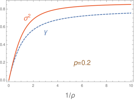
Figure 2. The growth rate $\gamma$ and the variance $\sigma^{2}$ for the product of type $n_{-}(t_{j})\,k(\tau_{j})$ discussed in §5.2, plotted against the mean value $1/\rho$ of $\tau_{j}$, for a fixed unit mean $1/p=5$ of $t_{j}$.

5.3. Products of the type $n_{-}\,n_{+}$

The perturbative analysis of products consisting of elements of the form

$$g_{j}=n_{-}(t_{j})\,n_{+}(\tau_{j})\,,$$

where $t_{j}$ and $\tau_{j}$ are as before, requires no further adjustment other than updating the definitions of the operators ${\mathscr{A}}_{0}$ and ${\mathscr{B}}$:

(5.13) $${\mathscr{A}}_{0}=\frac{1}{\chi(s)}\left(1-\frac{\text{i}s}{\rho}\frac{d^{2}}{ds^{2}}\right)\,,\;\;{\mathscr{B}}=\frac{1}{\chi(s)}\frac{2\text{i}}{\rho}\frac{d}{ds}\,.$$

This leads to the revised formulae

(5.14) $$\lambda_{1}=-\frac{2}{\rho}\,\text{Im}\left[f_{0}^{\prime}(0+)\right]$$

and

(5.15) $$\lambda_{2}=-\frac{2}{\rho}\,\lim_{s\rightarrow 0+}\text{Im}\left[f_{1}^{\prime}(s)\right]=2\int_{0}^{\infty}\frac{ds}{s}\,\text{Re}\left[\lambda_{1}\chi(s)f_{0}^{2}(s)-\frac{2\text{i}}{\rho}f_{0}(s)f_{0}^{\prime}(s)\right]\,.$$

As an illustration, we can solve Exercise 5.5 in [3], which corresponds to taking for $t_{j}$ an exponential distribution of mean $1/p$. The solution of the Dyson–Schmidt equation is

(5.16) $$f_{0}(s)=\frac{\sqrt{p-\text{i}s}\,K_{1}\left(2\sqrt{\rho\,(p-\text{i}s)}\right)}{\sqrt{p}\,K_{1}\left(2\sqrt{\rho\,p}\right)}\,.$$

It follows in particular that the invariant distribution is a generalised inverse Gaussian — a fact discovered by Letac & Seshadri [26]. After some straightforward manipulations, we deduce from Equations (1.23) and (5.14)

$$\gamma=-\frac{\lambda_{1}}{2}=\frac{1}{\sqrt{\rho\,p}}\,\frac{K_{0}\left(2\sqrt{\rho\,p}\right)}{K_{1}\left(2\sqrt{\rho\,p}\right)}\,.$$

Plots of $\gamma$ and of the variance $\sigma^{2}=\lambda_{1}^{2}/4-\lambda_{2}/2$ against $1/\rho$, for a fixed $p$, are shown in Figure 3.

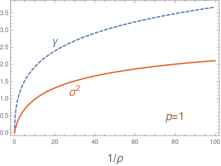
Figure 3. The growth rate $\gamma$ and the variance $\sigma^{2}$ for the product of type $n_{-}(t_{j})\,n_{+}(\tau_{j})$ discussed in §5.3, plotted against the mean value $1/\rho$ of $\tau_{j}$, for a fixed unit mean $1/p=1$ of $t_{j}$.

If we replace $\rho$ by $-\rho$, we recover the model studied by Kotani in [24], §5, Example 1, for which the Lyapunov exponent may be expressed in terms of a Hankel function.

5.4. Products of the type $n_{-}\,a_{1}$

The matrices are lower triangular in this case; the diagonal entries depend only on the $a_{1}$ component, and so the calculation of the generalised Lyapunov exponent is trivial. For instance, if $t_{j}$ is exponentially distributed with mean $1/p$, we deduce directly from the definition (1.3) that

$$\Lambda(2\ell)=-\ln\left(1-\frac{\ell}{\rho}\right)\;\;\text{for $\text{Re}\,\ell<\rho$}\,.$$

This simplification manifests itself in the fact that, as can be seen from the entries of Table 3, the inverse of the transfer operator

$${\mathscr{T}}_{\ell}^{-1}=\left(1-\frac{1}{\rho}{A}_{1}\right)\left(1-\frac{1}{p}{N}_{-}\right)$$

and hence also its adjoint ${\mathscr{A}}_{\ell}$ are both first-order differential operators:

$${\mathscr{T}}_{\ell}^{-1}=\left[1+\frac{1}{\rho}\left(s\frac{d}{ds}+\ell+1\right)\right]\left(1+\frac{\text{i}s}{p}\right)\,,\;\;{\mathscr{A}}_{\ell}=\left(1-\frac{\text{i}s}{p}\right)\left[1-\frac{1}{\rho}\left(s\frac{d}{ds}-\overline{\ell}\right)\right]\,.$$

Despite such simplicity, it turns out that the perturbative approach does not produce the correct result in this case. The Dyson–Schmidt equation

$$\frac{df_{0}}{ds}+\frac{\rho}{s+\text{i}p}f_{0}=0$$

is readily solved by separating the variables:

$$f_{0}(s)=c(s+\text{i}p)^{\rho}$$

for some constant $c$. But this function cannot be the Fourier transform of a probability density. We are in a situation where there is no measure on the Furstenberg boundary invariant for this product. The probability distribution on $\text{SL}(2,{\mathbb{R}})$ corresponding to this random product fails to satisfy Furstenberg’s “strong irreduciblity condition”. This condition says that the smallest subgroup containing the distribution’s support, acting on ${\mathbb{R}}^{2}$, should not leave invariant a finite union of one-dimensional subspaces [16]; without it, and without some other conditions, the existence of an invariant measure cannot be guaranteed. We refer the reader to [3], Theorem 4.1 and Proposition 4.3, for a useful list of such conditions.

If one changes the probability distribution so that it is now $-\tau_{j}$ that is exponentially distributed with mean $1/\rho$ then the generalised Lyapunov exponent does not change but the invariant measure does exist. Indeed, this change is tantamount to replacing $\rho$ by $-\rho$ in the Dyson–Schmidt equation; the solution is now given by

$$f_{0}(s)=\frac{c}{(s+\text{i}p)^{\rho}}$$

and, after normalisation, we recognise the Fourier transform of a gamma density. We can use the recurrence relation (1.20) with

$$v_{0}=\delta\;\;\text{and}\;\;{\mathscr{B}}=-\frac{1}{\rho}{I}$$

and the perturbative approach produces the correct result

$$\lambda_{1}=-\frac{1}{\rho}\;\;\text{and}\;\;\lambda_{2}=0\,.$$

6. Realisation on the hyperbola

For the diagonalisation of $T_{\ell}$ with respect to the subgroup $A_{1}$, it is convenient to work with the realisation on the two-branched hyperbola of equation

$$x_{2}=\frac{1}{|x_{1}|}\,.$$

To every $v\in V_{\ell}$, we associate the function $\widetilde{v}:\,{\mathbb{R}}_{\ast}\rightarrow{\mathbb{C}}$ defined by

$$\widetilde{v}(x):=v\left(\frac{x}{\sqrt{|x|}},\frac{1}{\sqrt{|x|}}\right)\,.$$

We denote by $Q$ the operator that assigns $\widetilde{v}$ to $v$ and define the space $\widetilde{V}_{\ell}$ of complex-valued functions on ${\mathbb{R}}_{\ast}$ by Equation (2.1). By making use of the identity

$$\widetilde{v}(x)=|x|^{-\ell}\,v(x,1)$$

we easily deduce the following from Lemma 4.1:

Lemma 6.1.

For $\widetilde{v}$ to belong to $\widetilde{V}_{\ell}$, it is necessary and sufficient that both the functions

$${\mathbb{R}}_{\ast}\ni x\mapsto|x|^{\ell}\,\widetilde{v}(x)\;\;\text{and}\;\;{\mathbb{R}}_{\ast}\ni x\mapsto|x|^{\ell}\,\widetilde{v}(1/x)$$

be smooth.

In particular, if $\widetilde{v}\in\widetilde{V}_{\ell}$, then the limits

$$\lim_{x\rightarrow\infty}|x|^{-\ell}\,\widetilde{v}(x)\;\;\text{and}\;\;\lim_{x\rightarrow-\infty}|x|^{-\ell}\,\widetilde{v}(x)$$

exist and are equal. Furthermore, the limit

$$\lim_{x\rightarrow 0}|x|^{\ell}\,\widetilde{v}(x)$$

also exists.

The map $Q:\,V_{\ell}\rightarrow\widetilde{V}_{\ell}$ is bijective and the representation $T_{\ell}$ is realised on the space $\widetilde{V}_{\ell}$ via Equation (2.2):

(6.1) $$\left[\widetilde{T}_{\ell}(g)\widetilde{v}\right](x):=\left|\frac{(ax+c)(bx+d)}{x}\right|^{\ell}\,\widetilde{v}\left(\frac{ax+c}{bx+d}\right)\,.$$

From now on, we shall omit the tilde.

We remark that the measure $dx/|x|$ is invariant under the action of the subgroup $A_{1}$. The corresponding multiplier is given by the formula

$$\sigma_{A_{1}}(x,g):=\frac{|x|}{\left|x\cdot g\right|}\frac{d}{dx}\left(x\cdot g\right)=\left|\frac{x}{(ax+c)(bx+d)}\right|$$

and so the realisation on the hyperbola may also be expressed as

(6.2) $$\left[T_{\ell}(g)v\right](x)=\sigma_{A_{1}}(x,g)^{-\ell}\,v(x\cdot g)\,.$$

6.1. The adjoint

For every $v\in V_{\ell}$ and every $f\in V_{\ell^{\ast}}$, we deduce from the asymptotic behaviours found above that

$$|x|\,\overline{f(x)}\,v(x)\xrightarrow[|x|\rightarrow\infty]{}C\;\;\text{and}\;\;\frac{1}{|x|}\overline{f(x)}\,v(x)\xrightarrow[x\rightarrow 0]{}c$$

for some constants $c$ and $C$ depending on $f$ and $v$. It follows that $f$ may be identified with the continuous linear functional defined on $V_{\ell}$ by

(6.3) $$v\mapsto\int_{{\mathbb{R}_{\ast}}}\overline{f(x)}\,v(x)\,\frac{dx}{|x|}=:\mathinner{\langle{f|v}\rangle}\,.$$

Hence

$$V_{\ell^{\ast}}\subset V_{\ell}^{\ast}\,.$$

It is then readily verified by direct calculation that the adjoint of $T_{\ell}$ with respect to this inner product is given by

(6.4) $$\left[T_{\ell}^{\ast}(g)f\right](x)=\sigma_{A_{1}}(x,g^{-1})^{-\ell^{\ast}}f(x\cdot g^{-1})\\ =\left|\frac{(dx-c)(a-bx)}{x}\right|^{\ell^{\ast}}\,f\left(\frac{dx-c}{a-bx}\right)\,.$$

The appropriate Hilbert space for the realisation on the hyperbola is thus

$$H:=\left\{v:\,{\mathbb{R}}_{\ast}\rightarrow{\mathbb{C}}:\,\int_{{\mathbb{R}}_{\ast}}|v(x)|^{2}\,\frac{dx}{|x|}<\infty\right\}$$

equipped with the inner product (6.3). In this realisation, $V_{\ell}\subset H$ only if $\text{Re}\,\ell<0$. The sequences

$$\{{\mathbf{e}}_{\ell^{\ast},m}\}_{m\in{\mathbb{Z}}}\subset V_{\ell^{\ast}}\;\;\text{and}\;\;\{{{\mathbf{e}}_{\ell,n}}\}_{n\in{\mathbb{Z}}}\subset V_{\ell}$$

constitute a bi-orthogonal system for this inner product.

6.2. Realisation in Mellin space

In order to diagonalise with respect to the subgroup $A_{1}$, we work with the realisation on the hyperbola. First, we assign, to every $v\in V_{\ell}$, the pair

$$(v_{+},\,v_{-}):\,(0,\infty)\rightarrow{\mathbb{C}}^{2}$$

where

$$v_{+}(x):=v(x)\;\;\text{and}\;\;v_{-}(x):=v(-x)\,,\;\;x>0\,.$$

We can assert that there exist constants $c$ and $C$, depending only on $v$, such that

$$v_{\pm}(x)\sim C\,x^{\ell}\;\;\text{as $x\rightarrow\infty$}\;\;\text{and}\;\;v_{\pm}(x)\sim c\,x^{-\ell}\;\;\text{as $x\rightarrow 0+$}\,.$$

It then follows that the Mellin transforms

$$\widehat{v}_{\pm}(s):=\int_{0}^{\infty}dx\,x^{\text{i}s-1}v_{\pm}(x)$$

exist, in the classical sense, in the strip

(6.5) $$\text{Re}\,\ell<\text{Im}\,s<-\text{Re}\,\ell\,.$$

We put

$$\widehat{v}:=(\widehat{v}_{+},\widehat{v}_{-})$$

and denote by $Q$ the operator that assigns $\widehat{v}$ to $v$. We may then obtain a new realisation $\widehat{T}_{\ell}$ of $T_{\ell}$ in the space

$$\widehat{V}_{\ell}:=\left\{Qv:\,v\in V_{\ell}\right\}$$

by setting

$$\widehat{T}_{\ell}\,Q=Q\,T_{\ell}\,.$$

We call this the realisation in Mellin space. In particular, for

$$g=\begin{pmatrix}e^{\frac{t}{2}}&0\\ 0&e^{-\frac{t}{2}}\end{pmatrix}\,,$$

we have

$$\left[T_{\ell}(g)v\right]_{\pm}(x)=v_{\pm}\left(e^{t}x\right)\;\;\text{for}\;x>0\,.$$

We readily deduce

$$\left[\widehat{T}_{\ell}(g)\widehat{v}\right](s)=e^{-\text{i}st}\,\widehat{v}(s)$$

and so this realisation is indeed diagonal with respect to the subgroup $A_{1}$.

We have defined the Mellin transform $\widehat{v}_{\pm}$ in such a way that it is, for $s$ real, the Fourier transform of the function ${\mathbb{R}}\ni t\mapsto v_{\pm}(e^{t})$. Parseval’s formula for the Fourier transform then leads to the identity

(6.6) $$\mathinner{\langle{f|v}\rangle}:=\int_{-\infty}^{\infty}\frac{dx}{|x|}\,\overline{f(x)}\,v(x)=\frac{1}{2\pi}\int_{-\infty}^{\infty}ds\left[\overline{\widehat{f}_{+}(s)}\,\widehat{v}_{+}(s)+\overline{\widehat{f}_{-}(s)}\,\widehat{v}_{-}(s)\right]$$

and we shall use the right-hand side as the definition of the inner product in $\widehat{V}_{\ell}$. This choice ensures the bi-orthogonality of $\{\widehat{\mathbf{e}}_{\ell^{\ast},m}\}_{m\in{\mathbb{Z}}}$ and $\{\widehat{\mathbf{e}}_{\ell,n}\}_{n\in{\mathbb{Z}}}$.

It is interesting to examine the form that the ${{\mathbf{e}}_{\ell,n}}$ assume when we go over to the realisation in Mellin space: By definition,

$${\mathbf{e}}_{\ell,n{\pm}}(x)=\frac{(-1)^{n}}{\sqrt{\pi}}\left(\frac{1\mp\text{i}x}{1\pm\text{i}x}\right)^{n}\left(x+\frac{1}{x}\right)^{\ell}\,.$$

Hence

$$\widehat{\mathbf{e}}_{\ell,n\pm}(s)=\frac{(-1)^{n}}{\sqrt{\pi}}\int_{0}^{\infty}dx\,x^{\text{i}s-\ell-1}(1\mp\text{i}x)^{\ell+n}(1\pm\text{i}x)^{\ell-n}\,.$$

The value of this integral is given by Formula 6.2.35 in [13]:

(6.7) $$\widehat{\mathbf{e}}_{\ell,n\pm}(s)=\frac{(-1)^{n}}{\sqrt{\pi}}\,e^{\pm\text{i}\frac{\pi}{2}(\ell-\text{i}s)}\,{\tt B}\left(-\ell+\text{i}s,\,-\ell-\text{i}s\right){{}_{2}}F_{1}\left(-\ell-n,\text{i}s-\ell;-2\ell;2\right)\,.$$

For $\ell\in\{-1,\,-2,\,\ldots\}$ and $n\geq-\ell$, the hypergeometric function in this formula may be expressed in terms of the Meixner–Pollaczek polynomials [23]. An alternative inner product may then be found that makes $\widehat{T}_{\ell}^{-}$ unitary.

It would be tedious to write down $\widehat{T}_{\ell}(g)$ explicitly for an arbitrary $g\in G$; see [41, 42]. For our purposes, we only need to know the infinitesimal generators associated with the various subgroups, and these can be worked out by taking the Mellin transform of the corresponding generator for $T_{\ell}$. Thus, for instance, in order to compute $\widehat{K}$, we use the fact that, for $x>0$,

$$\left({K}v\right)_{\pm}(x)=\left({K}v\right)(\pm x)=\pm\left[\frac{\ell}{2}\left(\frac{1}{x}-x\right)v_{\pm}(x)+\frac{1+x^{2}}{2}\,v_{\pm}^{\prime}(x)\right]\,.$$

If we then multiply each of these identities by $x^{\text{i}s-1}$ and integrate over $x$, we obtain

$$\left(\widehat{K}\,\widehat{v}\right)_{\pm}(s)=\pm\frac{1}{2}(\ell+1-\text{i}s)\,\widehat{v}_{\pm}(s+\text{i})\mp\frac{1}{2}(\ell+1+\text{i}s)\,\widehat{v}_{\pm}(s-\text{i})\,.$$

The other generators are listed in Table 4 where, as is our practice when there is no risk of confusion, we have dropped the hats.

$\left({K}\,{v}\right)_{\pm}(s)=\pm\frac{1}{2}(\ell+1-\text{i}s)\,{v}_{\pm}(s+\text{i})\mp\frac{1}{2}(\ell+1+\text{i}s)\,{v}_{\pm}(s-\text{i})$

$\left(A_{1}{v}\right)_{\pm}=-\text{i}s\,v_{\pm}(s)$

$\left(A_{2}\,{v}\right)_{\pm}(s)=\pm\frac{1}{2}(\ell+1-\text{i}s)\,{v}_{\pm}(s+\text{i})\pm\frac{1}{2}(\ell+1+\text{i}s)\,{v}_{\pm}(s-\text{i})$

$\left(N_{+}{v}\right)_{\pm}(s)=\pm\left(\ell+1+\text{i}s\right)v_{\pm}(s-\text{i})$

$\left(N_{-}{v}\right)_{\pm}(s)=\pm\left(\ell+1-\text{i}s\right)v_{\pm}(s+\text{i})$

Table 4. Infinitesimal generators associated with the realisation of $T_{\ell}$ in Mellin space.

Although in principle this realisation should be advantageous for the study of products involving the subgroup $A_{1}$, the difference operators that arise have the awkward feature that the increments are imaginary, whereas the auxiliary condition for the Dyson–Schmidt equation is that the solution should decay as the independent variable $s$ tends to infinity along the real axis. This makes it difficult to identify the correct solution without resorting to the realisation on the hyperbola; see [6] for examples of products of the type $a_{1}\,a_{2}$. This difficulty is exacerbated when we try to compute the next terms in the perturbation expansion.

7. Concluding remarks

In this paper, we have shown how the calculation of the Lyapunov exponent for certain probability distributions on the group $\text{SL}(2,{\mathbb{R}})$ can be carried out successfully by using a family of representations in a space of functions on the Furstenberg boundary. The cases that we studied are of interest as models of one-dimensional systems and led to simple formulae for the growth rate and the variance; we found that the special functions that appear in these formulae are the same as those that serve to express the basis functions in a suitable realisation of the representation space. One can reasonably expect that the calculation of the generalised Lyapunov exponent can be pushed further. Admittedly, the probability distributions considered here had very special features; in every case, essential use was made of the univariate exponential distribution, and it is not clear why this distribution should play a distinguished part in connection with $\text{SL}(2,{\mathbb{R}})$.

Furstenberg’s theory applies to a large class of semi-simple groups. For example, the Furstenberg boundary of the real symplectic group— which provides a generalisation of $\text{SL}(2,{\mathbb{R}})$ that is of particular interest in the context of disordered systems— is the (isotropic) flag manifold [4]. The so-called “degenerate principal series representations” are defined in spaces of functions on (parts of) that manifold and bear some resemblance with the family of representations considered here; they have been studied by Lee [25], following ideas put forward by Howe & Tan [22]. Likewise, Vilenkin’s ideas are not restricted to the group $\text{SL}(2,{\mathbb{R}})$ and have been developed extensively in recent years [42, 43]. One can therefore envisage the existence of special functions associated with other semi-simple groups that might be useful in the study of random products. It is apparent, however, that any extension of our results to larger groups would require a fairly detailed knowledge of their representation theory, as well as a high level of computational skill.

References

• [1] V. Bargmann, Irreducible unitary representations of the Lorentz group, Ann. Math. 48 (1947) 568–640.
• [2] Y. Benoist and J.-F. Quint, Random Walks on Reductive Groups, Springer, Berlin, 2016.
• [3] P. Bougerol and J. Lacroix, Products of Random Matrices with Applications to Schrödinger Operators, Birhaüser, Basel, 1985.
• [4] R. Carmona and J. Lacroix, Spectral Theory of Random Schrödinger Operators, Birkhaüser, Boston, 1990.
• [5] F. Comets, G. Giacomin and R. Greenblatt, Continuum limit of random matrix products in statistical mechanics of disordered systems, Commun. Math. Phys. 369 (2019) 171–219.
• [6] A. Comtet, C. Texier and Y. Tourigny, Supersymmetric quantum mechanics with Lévy disorder in one dimension, J. Stat. Phys. 145 (2011) 1291–1323.
• [7] A. Comtet, C. Texier and Y. Tourigny, Lyapunov exponents, one-dimensional Anderson localization and products of random matrices, J. Phys. A: Math. Theor. 46 (2013) 254003.
• [8] A. Crisanti, G. Paladin and A. Vulpiani, Products of random matrices in Statistical Physics, Springer–Verlag, Berlin, Heidelberg, 1993.
• [9] M. Davidson, G. Ólafsson and G. Zhang, Laguerre polynomials, restriction principle and holomorphic representations of $\text{SL}(2,{\mathbb{R}})$, Acta Appl. Math. 71 (2002) 261-277.
• [10] L. I. Deych, A. A. Lisyansky and B. L. Altshuler, Single parameter scaling in one-dimensional localization revisited, Phys. Rev. Lett. 84 (2000) 2678.
• [11] M. Drabkin and H. Schulz–Baldes, Gaussian fluctuations of products of random matrices distributed close to the identity, J. Difference Equ. Appl. 21 (2015), 467 485.
• [12] F. J. Dyson, The dynamics of a disordered chain, Phys. Rev. 92 (1953) 1331–1338.
• [13] A. Erdélyi (ed.) Tables of Integral Transforms, McGraw–Hill, New-York, 1954.
• [14] P. J. Forrester, Lyapunov exponents for products of complex Gaussian random matrices, J. Stat. Phys. 151 (2013) 796 808.
• [15] H. L. Frisch and S. P. Lloyd, Electron levels in a one-dimensional random lattice, Phys. Rev. 120 (1960) 1175–1189.
• [16] H. Furstenberg, Noncommuting random products, Trans. Amer. Math. Soc. 108 (1963) 377-428.
• [17] Y. V. Fyodorov, P. Le Doussal, A. Rosso and C. Texier, Exponential number of equilibria and depinning threshold for a directed polymer in a random potential, Ann. Phys. 397 (2018) 1-64.
• [18] I. M. Gel’fand, M. I. Graev and N. Ya. Vilenkin, Generalized Functions, Volume 5: Integral Geometry and Representation Theory, Academic Press, New-York, 1966.
• [19] I. M. Gel’fand and G. E. Shilov, Generalized Functions, Volume 1: Properties and Operations, Academic Press, New-York, 1966.
• [20] I. S. Gradshteyn and I. M. Ryzhik, Table of Integrals Series and Products, Academic Press, New-York, 1965.
• [21] B. I. Halperin, Green’s functions for a particle in a one-dimensional potential, Phys. Rev. 139 (1965) A104–A117.
• [22] R. E. Howe and E. C. Tan, Homogeneous functions on light cones: The infinitesimal structure of some degenerate principal series representations, Bull. Amer. Math. Soc. 28 (1993) 1–74.
• [23] T. H. Koornwinder, Meixner–Pollaczek polynomials and the Heisenberg algebra, J. Math. Phys. 30 (1989) 767–769.
• [24] S. Kotani, On asymptotic behaviour of the spectra of a one-dimensional Hamiltonian with a certain random coefficient, Publ. RIMS, Kyoto Univ. 12 (1976) 447-492.
• [25] S. T. Lee, Degenerate principal series representations of $\text{Sp}(2n,{\mathbb{R}})$, Compositio Math. 103 (1996) 123 151.
• [26] G. Letac and V. Seshadri, A characterixation of the generalixed inverse Gaussian distribution by continued fractions, Z. Wahrscheinlichkeitstheorie verw. Gebiete 62 (1983), 485-489.
• [27] G. Lindblad and B. Nagel, Continuous bases for unitary irreducible representations of $\text{SU}(1,1)$, Ann. Inst. Henri Poincaré A, 13 (1970), 27–56.
• [28] D. R. Masson, Difference equations, continued fractions, Jacobi matrices and orthogonal polynomials, in Nonlinear Numerical Methods and Rational Approximation, 239–257, A. Cuyt (ed.), D. Reidel Publishing Company, 1988.
• [29] Yu. A. Neretin, Difference Sturm–Liouville problems in the imaginary direction, J. Spectr. Theory 3 (2013), 237–269.
• [30] C. M. Newman, The distribution of Lyapunov exponents: exact results for random matrices, Commun. Math. Phys. 103 (1986) 121-126.
• [31] T. M. Nieuwenhuizen, Exact electronic spectra and inverse localization lengths in one-dimensional random systems: I. Random alloy, liquid metal and liquid alloy, Physica 120A (1983) 468-514.
• [32] M. Pollicott, Maximal Lyapunov exponents for random matrix products, Inv. Math. 181 (2010) 209-226.
• [33] F. W. J. Olver, A. B. Olde Daalhuis, D. W. Lozier, B. I. Schneider, R. F. Boisvert, C. W. Clark, B. R. Miller, and B. V. Saunders (eds), NIST Digital Library of Mathematical Functions, http://dlmf.nist.gov/, Release 1.0.23 of 2019-06-15.
• [34] K. Ramola and C. Texier, Fluctuations of random matrix products and 1d Dirac equation with random mass, J. Stat. Phys. 157 (2014) 497 514.
• [35] H. Schmidt, Disordered one-dimensional crystals, Phys. Rev 105 (1957) 425-441.
• [36] H. Schomerus and M. Titov, Statistics of finite-time Lyapunov exponents in a random time-dependent potential, Phys. Rev. E 66 (2002) 066207.
• [37] H. Schomerus and M. Titov, Anomalous wave function statistics on a one-dimensional lattice with power-law disorder, Phys. Rev. Lett. 91 (2003) 176601.
• [38] C. Texier, Fluctuations of the product of random matrices and generalised Lyapunov exponent, submitted to J. Stat. Phys. (2019). https://arxiv.org/pdf/1907.08512.pdf
• [39] V. N. Tutubalin, On limit theorems for the product of random matrices, Theor. Prob. Appl. 10 (1965) 15-27.
• [40] J. Vanneste, Estimating generalized Lyapunov exponents for products of random matrices, Phys. Rev. E 81 (2010) 036701.
• [41] N. Ja. Vilenkin, Special Functions and the Theory of Group Representations, American Mathematical Society, 1968.
• [42] N. Ja. Vilenkin and A. U. Klimyk, Representations of Lie Groups and Special Functions, Volume 1: Simplest Lie Groups, Special Functions and Integral Transforms, Kluwer, Dordrecht, 1991.
• [43] N. Ja. Vilenkin and A. U. Klimyk, Representations of Lie Groups and Special Functions, Volume 3: Classical and Quantum Groups and Special Functions, Kluwer, Dordrecht, 1992.
• [44] M. I. Vishik and L. A. Lyusternik, The solution of some perturbation problems for matrices and selfadjoint or non-selfadjoint differential equations I, Russ. Math. Surv. 15 (1960) 1–73.
• [45] R. Zillmer and A. Pikovsky, Multiscaling of noise-induced parametric instability, Phys. Rev. E 67 (2003) 061117.