Asymptotics for the nodal components
of non-identically distributed
monochromatic random waves

Abstract.

We study monochromatic random waves on $\mathbb{R}^{n}$ defined by Gaussian variables whose variances tend to zero sufficiently fast. This has the effect that the Fourier transform of the monochromatic wave is an absolutely continuous measure on the sphere with a suitably smooth density, which connects the problem with the scattering regime of monochromatic waves. In this setting, we compute the asymptotic distribution of the nodal components of random monochromatic waves, showing that the number of nodal components contained in a large ball $B_{R}$ grows asymptotically like $R/\pi$ with probability $p_{n}>0$, and is bounded uniformly in $R$ with probability $1-p_{n}$ (which is positive if and only if $n\geqslant 3$). In the latter case, we show the existence of a unique noncompact nodal component. We also provide an explicit sufficient stability criterion to ascertain when a more general Gaussian probability distribution has the same asymptotic nodal distribution law.

1. Introduction

The Nazarov–Sodin theory, whose original motivation was to understand the nodal set of random spherical harmonics of large order [NS09], has been significantly extended to derive asymptotic laws for the distribution of the zero set of smooth Gaussian functions of several variables. The primary examples are the restriction to large balls of translation-invariant Gaussian functions on $\mathbb{R}^{n}$ and various Gaussian ensembles of large-degree polynomials on the sphere or on the torus.

From the point of view of applications, a particularly relevant problem that falls within this framework is that of monochromatic random waves, that is, solutions to the Helmholtz equation on $\mathbb{R}^{n}$ ($n\geqslant 2$):

$$\Delta u+u=0\,.$$ (1.1)

Since it is well known that any polynomially bounded solution to this equation is the Fourier transform of a distribution supported on the unit sphere $\SS$, the way one constructs monochromatic random waves is the following [CS19]. One starts with a real-valued orthonormal basis of spherical harmonics on $\SS$, which we denote by $Y_{lm}$. Hence $Y_{lm}$ is an eigenfunction of the spherical Laplacian with eigenvalue $l(l+n-2)$, the index $l$ is a nonnegative integer and $m$ ranges from 1 to the multiplicity $d_{l}:=\frac{2l+n-2}{l+n-2}\binom{l+n-2}{l}$ of the corresponding eigenvalue.

To consider a monochromatic random wave, one now takes

$$f(\xi):=\sum_{l=0}^{\infty}\sum_{m=1}^{d_{l}}i^{l}\,a_{{l}m}\,Y_{lm}(\xi)\,,$$ (1.2a)

where $$a_{lm} u f\,dS dS \SS$$ are independent random variables, and defines  as the Fourier transform of , where is the area measure of the unit sphere . This is tantamount to setting

$$u(x)=(2\pi)^{\frac{n}{2}}\sum_{l=0}^{\infty}\sum_{m=1}^{d_{l}}a_{lm}\,Y_{lm}\bigg{(}\frac{x}{|x|}\bigg{)}\,\frac{J_{l+\frac{n}{2}-1}(|x|)}{|x|^{\frac{n}{2}-1}}\,,$$ (1.2b)

Note that $u$ is real-valued if the random variables $a_{lm}$ are. In the Nazarov–Sodin theory, one assumes that the random variables $a_{lm}$ are independent standard Gaussians (i.e., of zero mean and unit variance).

Let us denote by $N_{u}(R)$ (resp., $N_{u}(R;[\Sigma])$) the number of connected components of the nodal set $u^{-1}(0)$ that are contained in the ball centered at the origin of radius $R$ (resp., and diffeomorphic to $\Sigma$). Here $\Sigma$ is any smooth, closed, orientable hypersurface $\Sigma\subset\mathbb{R}^{n}$. It is obvious from the definition that $N_{u}(R;[\Sigma])$ only depends on the diffeomorphism class $[\Sigma]$ of the hypersurface. The central known results concerning the asymptotic distribution of the nodal components of monochromatic random waves can then be summarized as follows (see also [GW16, KW18, CS19] for related results):

Theorem 1.1.

Suppose that the random variables $a_{lm}$ in Equation (1.2) are independent standard Gaussian variables. Then:

1. Nazarov–Sodin’s estimate for the number of nodal components [NS16]: There is a constant $\nu>0$ such that

   $$\mathbb{P}\Bigg{(}\lim_{R\to\infty}\frac{N_{u}(R)}{R^{n}}=\nu\Bigg{)}=1\,.$$

2. Sarnak–Wigman’s positive probability bound for the number of nodal sets of fixed topology [SW19]: For each smooth, closed, orientable hypersurface $\Sigma\subset\mathbb{R}^{n}$ there exists a constant $\nu([\Sigma])>0$, depending only on the diffeomorphism class of $\Sigma$, such that

   $$\mathbb{P}\Bigg{(}\lim_{R\to\infty}\frac{N_{u}(R;[\Sigma])}{R^{n}}=\nu([\Sigma])\Bigg{)}=1\,.$$

Remark 1.2.

More visually, this theorem asserts that, if $a_{lm}$ are independent standard Gaussians, the number of nodal components contained in a large ball is almost surely proportional to the volume. This volumetric growth rate holds even if one only considers nodal components of a fixed (compact) topology.

Our objective in this paper is to understand the asymptotic distribution of the nodal set of $u$ when the random variables $a_{lm}$, which we will no longer assume to be identically distributed, have different distribution laws. One obvious motivation to consider this problem is that the Helmholtz equation (1.1) plays a central role in Physics, particularly in quantum mechanics and electromagnetic theory via scattering problems and in stationary solutions of the 3D Euler equation through Beltrami fields [CK92, EPS15, RS79]. In these contexts (which are clearly different from the study of high energy eigenfunctions on a compact manifold and from problems in percolation theory), one is interested in solutions with the sharp decay at infinity, which is captured by imposing that the Agmon–Hörmander seminorm

$${\left|\kern-1.07639pt\left|\kern-1.07639pt\left|u\right|\kern-1.07639pt\right|\kern-1.07639pt\right|}:=\limsup_{R\to\infty}\bigg{(}\frac{1}{R}\int_{B_{R}}|u|^{2}\,dx\bigg{)}^{\frac{1}{2}}$$

is finite. As we recall in Appendix A, the decay properties of $u$ are closely related to the regularity of the function $f$ above; indeed, it is a classical result of Herglotz [Hör15, Theorem 7.1.28] that ${\left|\kern-1.07639pt\left|\kern-1.07639pt\left|u\right|\kern-1.07639pt\right|\kern-1.07639pt\right|}<\infty$ if and only if $u$ is the Fourier transform of a measure of the form $f\,dS$ with $\|f\|_{L^{2}(\SS)}<\infty$.

However, it is easy to see that, when $a_{lm}\sim\mathcal{N}(0,1)$ are standard Gaussians, $f$ is almost surely not in $L^{2}(\SS)$ by the law of large numbers. This means that this choice of random variables is very well suited to the study of random eigenfunctions on a compact manifold, as it is known since Nazarov and Sodin’s breakthrough paper on spherical harmonics [NS09], but precisely for this reason, it cannot capture the features of random solutions to non-compact problems in the scattering regime (i.e., with finite Agmon–Hörmander seminorm). Hence one would like to consider, at least, the case where

$$a_{lm}\sim\mathcal{N}(0,\sigma_{l}^{2})$$

are independent Gaussian variables of zero mean but distinct variances $\sigma_{l}^{2}$. The fall-off (or growth) of the covariance $\sigma_{l}$ as $l\to\infty$ is directly related to the expected regularity of $f$; indeed, the easiest calculation in this direction is that the expected value of the $H^{s}(\SS)$ norm of $f$ is

$$\mathbb{E}(\|f\|_{H^{s}(\SS)}^{2})=\sum_{l=0}^{\infty}{d_{l}}(1+l)^{2s}\sigma_{l}^{2}\,.$$ (1.3)

Since $d_{l}=c_{n}l^{n-2}+O(l^{n-3})$ for large $l$, a convenient way of stating our main result is as follows:

Theorem 1.3.

Suppose that the random variables $a_{lm}$ in Equation (1.2) are independent Gaussians $\mathcal{N}(0,\sigma_{l}^{2})$, where the variances satisfy

$$\sum_{l=0}^{\infty}(1+l)^{2s+n-2}\sigma_{l}^{2}<\infty$$ (1.4)

for some $s>\frac{n+5}{2}$. Then $f\in H^{s}(\SS)$ almost surely, so in particular ${\left|\kern-1.07639pt\left|\kern-1.07639pt\left|u\right|\kern-1.07639pt\right|\kern-1.07639pt\right|}<\infty$. Furthermore:

1. There exists some probability $p_{n}$, with $p_{2}=1$ and $p_{n}\in(0,1)$ if $n\geqslant 3$, such that

   $$\mathbb{P}\bigg{(}\lim_{R\to\infty}\frac{N_{u}(R)}{R}=\frac{1}{\pi}\bigg{)} =p_{n}\,,$$

   $$\mathbb{P}\bigg{(}\lim_{R\to\infty}{N_{u}(R)}<\infty\bigg{)} =1-p_{n}\,.$$

2. If $\Sigma\subset\mathbb{R}^{n}$ is a smooth, compact, orientable hypersurface, then

   $$\mathbb{P}\bigg{(}\lim_{R\to\infty}\frac{N_{u}(R;[\Sigma])}{R}=\frac{1}{\pi}\bigg{)} =p_{n} \text{if }[\Sigma]=[\SS]\,,$$

   $$\mathbb{P}\bigg{(}\lim_{R\to\infty}{N_{u}(R;[\Sigma])}<\infty\bigg{)} =1-p_{n} \text{if }[\Sigma]=[\SS]\,,$$

   $$\mathbb{P}\bigg{(}\lim_{R\to\infty}{N_{u}(R;[\Sigma])}<\infty\bigg{)} =1 \text{if }[\Sigma]\neq[\SS]\,.$$

Remark 1.4.

In plain words, this theorem says that, when the variances satisfy the convergence condition (1.4), the asymptotic distribution is completely different from that of the Nazarov–Sodin regime: the number of nodal components diffeomorphic to a sphere that are contained in a large ball grows like the radius with probability $p_{n}$ and stays uniformly bounded with probability $1-p_{n}$. The number of non-spherical nodal components stays uniformly bounded almost surely. One can also study the nesting graph of the nodal structure, see [SW19, BMW19] for a definition. In the setting of Theorem 1.3, with probability $p_{n}$, the nesting graph is a tree with degree 2 internal vertices, and the number of other trees is bounded almost surely.

Remark 1.5.

Arguing as in Lemma 4.2 using Equation (4.1), it is easy to show that the covariance kernel of our random field is

$$\mathbb{E}\left(u(x)u(y)\right)=(2\pi)^{n}\sum_{{l}=0}^{\infty}\sigma_{l}^{2}\frac{|d_{l}|}{|\SS|}P_{{l}n}\left(\frac{x}{|x|}\cdot\frac{y}{|y|}\right)\frac{J_{{l}+\frac{n}{2}-1}(|x|)}{|x|^{\frac{n}{2}-1}}\frac{J_{{l}+\frac{n}{2}-1}(|y|)}{|y|^{\frac{n}{2}-1}}\,,$$

where $P_{{l}n}$ is the Legendre polynomial of degree ${l}$ in $n$ dimensions. Therefore, our random field is isotropic (i.e., invariant under rotations) but not translation-invariant, in general. In the case when $\sigma_{{l}}=1$ for all ${l}$, one does have translational invariance; indeed, a straightforward computation [CS19] shows that the covariance kernel reduces to

$$\frac{J_{\frac{n}{2}-1}(|x-y|)}{|x-y|^{\frac{n}{2}-1}}$$

up to a multiplicative constant.

To offer some perspective into the ideas behind Theorem 1.3, it is convenient to start by recalling the gist of the proof of the first part of Theorem 1.1. Nazarov and Sodin start off with a clever (non-probabilistic) “sandwich estimate” of the form

$$\bigg{(}1-\frac{r}{R}\bigg{)}^{n}\mathop{\text{\makebox[0.0pt][l]{\makebox[4.16669pt]{$-$}}$\int$}}_{B_{R-r}}\frac{N_{\tau_{x}u}(r)}{r^{n}}\,dx\leqslant\frac{N_{u}(R)}{R^{n}}\leqslant\bigg{(}1+\frac{r}{R}\bigg{)}^{n}\mathop{\text{\makebox[0.0pt][l]{\makebox[4.16669pt]{$-$}}$\int$}}_{B_{R+r}}\frac{N_{\tau_{x}u}(r)+\mathfrak{N}_{\tau_{x}u}(r)}{r^{n}}\,dx\,,$$

where $\tau_{x}u(y):=u(x+y)$ is a translation of $u$ and $\mathfrak{N}_{u}(r)$ denotes the number of critical points of the restriction $u|_{\partial B_{r}}$. Now one can exploit the fact that, in the particular case when $a_{lm}$ are independent standard Gaussians, $u$ is a Gaussian random function with translation-invariant distribution, which is the setting that the Nazarov–Sodin theory applies to. Moreover, its spectral measure (which is simply $dS$, the normalized area measure on $\SS$) has no atoms. Therefore, a theorem of Grenander, Fomin and Maruyama and the Kac–Rice bound respectively imply that the action of shifts on $u$ is ergodic and that the expected value of $\mathfrak{N}_{u}(r)$ is of order $r^{n-1}$. By taking limits $1\ll r\ll R$, this readily implies the existence of $\lim_{R\to\infty}N_{u}(R)/R^{n}$. The fact that this limit is positive then follows from the sandwich estimate and the existence of a (non-random) solution with a structurally stable compact nodal set. Let us stress that the whole theory hinges on the fact that $a_{lm}$ are Gaussians of the same variance, as this is crucially employed both to connect the problem with the theory of Gaussian random functions and to show that one can compute limits using ergodic theory. The second item in Theorem 1.1 uses that, in fact, one can prescribe the topology of a robust nodal component [EPS13].

It should then come as no surprise that the proof of Theorem 1.3 is based on entirely different principles. The basic idea is that, with probability 1, in the setting of Theorem 1.3 the density $f$ is an $H^{s}(\SS)$-smooth function (and, as $s>\frac{n+5}{2}$, of class $C^{3}$ by the Sobolev embedding theorem) with nondegenerate zeros, and that the probability $p_{n}$ that $f$ does not vanish is strictly positive. When $f\in H^{s}(\SS)$ does not vanish, it is not hard to prove using asymptotic expansions that the number of nodal components contained in a large ball $B_{R}$ grows as the radius, and that all but a uniformly bounded number of them are diffeomorphic to a sphere. When the zero set of $f$ is regular and nonempty, one can show that the number of nodal components on $\mathbb{R}^{n}$ is bounded. However, the analysis is considerably subtler because it hinges on the stability of certain noncompact components of the nodal set that locally look like a helicoid. Putting these facts together, one heuristically arrives at Theorem 1.3.

It is worth mentioning that the regularity effect that we have striven to capture is completely different from the use of frequency-dependent weights considered by Rivera in the context of random Gaussian fields on compact manifolds [Riv19] (see also [FLL15] for frequency-dependent weights in the context of random algebraic hypersurfaces). Indeed, Rivera’s central result is that the Nazarov–Sodin asymptotics still holds, with different constants, for series of the form

$$F(x):=\sum_{k=1}^{L}\lambda_{k}^{-s}\,a_{k}\,e_{k}(x)\,,$$

where $L\gg 1$, $(e_{k},\lambda_{k})$ are the eigenfunctions and eigenvalues of the Laplacian on a compact $n$-manifold, $s\in(0,\frac{n}{2})$ and $a_{l}\sim\mathcal{N}(0,1)$. In contrast, we are interested in regimes with a different asymptotic behavior that correspond to a scattering situation on $\mathbb{R}^{n}$.

It is natural to wonder which kind of asymptotic laws may arise from more general randomizations of the function $f$. As a first step in this direction, we state next a “stability result”, that is, sufficient conditions for the asymptotics of Theorems 1.1 and 1.3 to hold for more general probability measures on the space of functions $f$ (or $u$). These conditions are by no means obvious a priori, but the proof is based on an elementary idea: if two probability measures $\mu$ and $\widetilde{\mu}$ (on the space of functions on the sphere, which one can identify with a space of sequences $\mathbb{R}^{\mathbb{N}}$) are equivalent (i.e., mutually absolutely continuous), then these measures have the same zero-probability events. The aforementioned sufficient conditions are then derived by imposing that one of these measures correspond to the Nazarov–Sodin distribution or to the distributions considered in Theorem 1.3.

Theorem 1.6.

Suppose that there is a nonnegative integer $l_{0}$ and reals $M_{lm}$ and $\sigma_{lm}$ such that the random variables $a_{lm}$ in Equation (1.2), which we assume to be independent, follow any probability distribution on the line (absolutely continuous with respect to the Lebesgue measure) for $l<l_{0}$ and Gaussian distributions $\mathcal{N}(M_{lm},\sigma_{lm}^{2})$ for $l\geqslant l_{0}$. Then:

1. The results of Theorem 1.1 hold, with the same constant $\nu$, if

   $$\sum_{{l}=l_{0}}^{\infty}\sum_{m=0}^{d_{l}}\Bigg{[}\frac{M_{lm}^{2}}{\sigma_{{l}m}^{2}+1}+\frac{(\sigma_{lm}-1)^{2}}{\sigma_{lm}}\Bigg{]}<\infty\,.$$

2. The results of Theorem 1.3 hold if there are constants $\sigma_{l}$ satisfying (1.4) such that

   $$\sum_{{l}=l_{0}}^{\infty}\sum_{m=0}^{d_{l}}\bigg{[}\frac{M_{lm}^{2}}{\left(\sigma_{l}^{2}+\sigma_{lm}^{2}\right)}+\frac{(\sigma_{{l}}-\sigma_{lm})^{2}}{\sigma_{{l}}\sigma_{lm}}\bigg{]}<\infty\,.$$

2. The Fourier transform of measures on the sphere with an $H^{s}$-smooth density

Our goal in this section is to obtain sharp asymptotic expansions for the Fourier transform

$$u:=\widehat{f\,dS}$$

of measures of the form $f\,dS$, where for the time being we can think of the integrable function $f:\SS\to\mathbb{C}$ simply as a series of spherical harmonics:

$$f(\xi):=\sum_{l=0}^{\infty}\sum_{m=1}^{d_{l}}f_{{l}m}\,Y_{lm}(\xi)\,.$$

It is well known that, for any real $s$, the $H^{s}(\SS)$ norm of $f$ can then be computed as

$$\|f\|_{H^{s}(\SS)}^{2}=\sum_{l=0}^{\infty}\sum_{m=1}^{d_{l}}(1+l)^{2s}|f_{{l}m}|^{2}\,.$$

We want $u$ to be real-valued, so we impose that

$$f_{lm}:=i^{l}a_{lm}$$

with $a_{lm}\in\mathbb{R}$. The real and imaginary parts of $f$ are then respectively given by the terms where $l$ is even and odd:

$$f_{\mathrm{R}}(\xi) :=\sum_{l\text{ even}}\sum_{m=1}^{d_{l}}(-1)^{\frac{l}{2}}a_{{l}m}\,Y_{lm}(\xi)\,,$$

$$f_{\mathrm{I}}(\xi) :=\sum_{l\text{ odd}}\sum_{m=1}^{d_{l}}(-1)^{\frac{l-1}{2}}a_{{l}m}\,Y_{lm}(\xi)\,.$$

To analyze $u$, we shall start by recalling the explicit formula for the Fourier transform of a spherical harmonic, which we borrow from [CS19]. For the benefit of the reader, we include a short proof that only employs classical formulas for special functions, instead of the theory of point pair invariants and zonal spherical functions. For the ease of notation, here and in what follows we set

$$\Lambda:=\frac{n}{2}-1\,.$$

Also, throughout we will often denote the radial and angular parts of $x$ by

$$r:=|x|\in\mathbb{R}^{+}\,,\qquad\theta:=\frac{x}{|x|}\in\SS\,.$$

Proposition 2.1.

The Fourier transform of the measure $Y_{lm}\,dS$ is

$$\widehat{Y_{{l}m}\,dS}(x)=(2\pi)^{\frac{n}{2}}\,(-i)^{l}\,Y_{{l}m}\left(\frac{x}{|x|}\right)\frac{J_{{l}+\Lambda}(|x|)}{|x|^{\Lambda}}\,,$$ (2.1)

where $J_{\alpha}$ is the Bessel function of the first kind.

Proof.

By the Funk–Hecke formula [AH12, Theorem 2.22], we have

$$\widehat{Y_{{l}m}\,dS}(x)=c_{{l}}(r)Y_{{l}m}(\theta)\,,$$ (2.2)

where

$$c_{{l}}(r)=|\mathbb{S}^{n-2}|\int_{-1}^{1}e^{-itr}\,P_{{l}n}(t)(1-t^{2})^{\frac{n-3}{2}}\,dt\,.$$ (2.3)

Here $P_{{l}n}$ is the Legendre polynomial. In turn, this last integral can be calculated using the formula [AH12, Proposition 2.26]:

$$\int_{-1}^{1}e^{-itr}\,P_{ln}(t)\,(1-t^{2})^{\frac{n-3}{2}}\,dt=\frac{(-ir)^{l}\,\Gamma(\frac{n-1}{2})}{2^{l}\Gamma(l+\frac{n-1}{2})}\int_{-1}^{1}e^{-itr}(1-t^{2})^{l+\Lambda-\frac{1}{2}}\,dt\,.$$

The proposition then follows in view of the well-known integral representation of the Bessel function,

$$J_{\alpha}\left(z\right)=\frac{(\tfrac{z}{2})^{\alpha}}{\pi^{\frac{1}{2}}\Gamma\left(\alpha+\tfrac{1}{2}\right)}\int_{-1}^{1}e^{-itz}\,(1-t^{2})^{\alpha-\frac{1}{2}}\,{d}t,$$ (2.4)

∎

While the obtention of an asymptotic expansion for the Fourier transform of the measure $f\,dS$ hinges on the analysis of oscillatory integrals, it is convenient to employ the structure of the problem to obtain sharper results. This will be done by exploiting the expansion in spherical harmonics and then using asymptotics with uniform constants directly for Bessel functions. It is worth pointing out that, by blindly following the general approach to asymptotic expansions (e.g., [Hör15, Theorem 7.7.14]), one would need $f\in H^{s}(\SS)$ with $s>\frac{3n+1}{2}$ (without considering derivatives), while the approach we take here will lower this number to $s>\frac{n+5}{2}$.

Let us denote by

$$\partial_{r}u:=\frac{x}{|x|}\cdot\nabla u\,,\qquad\not{\nabla}u:=\nabla u-\frac{x\cdot\nabla u}{|x|^{2}}x$$

the radial and angular parts of the gradient. The covariant derivative on the unit sphere will be denoted by $\nabla_{\mathbb{S}}$.

Proposition 2.2.

If $f\in H^{s}(\SS)$ with $s>\frac{n+5}{2}$, then

$$u =\frac{2(2\pi)^{\frac{n-1}{2}}}{r^{\frac{n-1}{2}}}\big{[}f_{\mathrm{R}}(\theta)\,\cos(r-r_{0})+f_{\mathrm{I}}(\theta)\,\sin(r-r_{0})+\mathcal{E}_{1}(r)\big{]}\,,$$

$$\partial_{r}u =\frac{2(2\pi)^{\frac{n-1}{2}}}{r^{\frac{n-1}{2}}}\big{[}-f_{\mathrm{R}}(\theta)\,\sin(r-r_{0})+f_{\mathrm{I}}(\theta)\,\cos(r-r_{0})+\mathcal{E}_{2}(r)\big{]}\,,$$

$$\not{\nabla}u =\frac{2(2\pi)^{\frac{n-1}{2}}}{r^{\frac{n+1}{2}}}\big{[}\nabla_{\mathbb{S}}f_{\mathrm{R}}(\theta)\,\cos(r-r_{0})+\nabla_{\mathbb{S}}f_{\mathrm{I}}(\theta)\,\sin(r-r_{0})+\mathcal{E}_{3}(r)\big{]}\,,$$

where $r_{0}:=\frac{\pi}{4}(n-1)$ and the errors are bounded as

$$|\mathcal{E}_{1}(x)|+|\nabla\mathcal{E}_{1}(x)|+|\mathcal{E}_{2}(x)|+|\mathcal{E}_{3}(x)|\leqslant\frac{C\|f\|_{H^{s}(\SS)}}{r}\,.$$

Proof.

By Proposition 2.1, $u$ is given by the series

$$u(x) =\sum_{l=0}^{\infty}\sum_{m=1}^{d_{l}}i^{l}a_{lm}\widehat{Y_{lm}\,dS}(x)$$

$$=\frac{(2\pi)^{\frac{n}{2}}}{r^{\Lambda}}\sum_{l=0}^{\infty}\sum_{m=1}^{d_{l}}a_{lm}Y_{lm}(\theta)\,{J_{l+\Lambda}(r)}\,.$$

Let us now recall the following uniform bound for a Bessel function [Kra14, Theorem 4], valid for all $\alpha\geqslant 0$ and $z\geqslant 0$:

$$J_{\alpha}(z)=\sqrt{\frac{2}{\pi z}}\,\cos\bigg{(}z-\frac{\pi\alpha}{2}-\frac{\pi}{4}\bigg{)}+\bigg{|}\alpha^{2}-\frac{1}{4}\bigg{|}\,\theta_{\alpha}(z)\,z^{-3/2}\,,$$ (2.5)

where $|\theta_{\alpha}(z)|\leqslant 1$. Setting

$$u_{1}(x) :=\frac{2(2\pi)^{\frac{n-1}{2}}}{r^{\frac{n-1}{2}}}\sum_{l=0}^{\infty}\sum_{m=1}^{d_{l}}a_{lm}Y_{lm}(\theta)\,\cos\bigg{(}r-r_{0}-\frac{\pi l}{2}\bigg{)}$$

$$\phantom{:}=\frac{2(2\pi)^{\frac{n-1}{2}}}{r^{\frac{n-1}{2}}}\big{[}f_{\mathrm{R}}(\theta)\,\cos(r-r_{0})+f_{\mathrm{I}}(\theta)\,\sin(r-r_{0})\big{]}\,,$$

it then follows that

$$\mathcal{E}_{1}(x):=\frac{r^{\frac{n-1}{2}}}{2(2\pi)^{\frac{n-1}{2}}}\,[u(x)-u_{1}(x)]$$

can be estimated as

$$|\mathcal{E}_{1}(x)| \leqslant\frac{C}{r}\sum_{l=0}^{\infty}\sum_{m=1}^{d_{l}}(l+1)^{2}|a_{lm}||Y_{lm}(\theta)|\,.$$

Using the Cauchy-Schwarz inequality, we then infer

$$|\mathcal{E}_{1}(x)|\leqslant\frac{C}{r}\sum_{l=0}^{\infty}(1+l)^{2}\bigg{(}\sum_{m=1}^{d_{l}}|Y_{lm}|^{2}\bigg{)}^{1/2}\bigg{(}\sum_{m=1}^{d_{l}}|a_{lm}|^{2}\bigg{)}^{1/2}\,.$$

The addition theorem [AH12, Theorem 2.9] ensures that, at any point on the sphere,

$$\sum_{m=1}^{d_{l}}|Y_{lm}|^{2}=c_{ln}$$ (2.6)

with an explicit constant bounded as $c_{nl}\leqslant C(l+1)^{n-2}$. This then allows us to write

$$|\mathcal{E}_{1}(x)|\leqslant\frac{C}{r}\sum_{l=0}^{\infty}(1+l)^{\frac{n}{2}+1}\bigg{(}\sum_{m=1}^{d_{l}}|a_{lm}|^{2}\bigg{)}^{1/2}\,.$$

Applying Cauchy–Schwarz again we obtain

$$|\mathcal{E}_{1}(x)|\leqslant\frac{C}{r}\bigg{(}\sum_{l=0}^{\infty}(1+l)^{n-2s+2}\bigg{)}^{1/2}\bigg{(}\sum_{l=0}^{\infty}\sum_{m=1}^{d_{l}}(1+l)^{2s}|a_{lm}|^{2}\bigg{)}^{1/2}\leqslant\frac{C}{r}\|f\|_{H^{s}(\SS)}\,,$$

as claimed.

Let us now compute the radial derivative of $u$. We start by noting that

$$\partial_{r}u={(2\pi)^{\frac{n}{2}}}\sum_{l=0}^{\infty}\sum_{m=1}^{d_{l}}a_{lm}\partial_{r}\bigg{[}Y_{lm}(\theta)\,\frac{J_{l+\Lambda}(r)}{r^{\Lambda}}\bigg{]}\,.$$

Since

$$\partial_{r}\bigg{(}\frac{J_{l+\Lambda}(r)}{r^{\Lambda}}\bigg{)}=\frac{J_{l+\Lambda-1}(r)}{r^{\Lambda}}-(l+2\Lambda)\,\frac{J_{l+\Lambda}(r)}{r^{\Lambda+1}}$$ (2.7)

and this formula depends solely on Bessel functions, one can now use again the uniform estimate Equation (2.5) to derive, with the same reasoning as above, that the error

$$\mathcal{E}_{2}(x):=\frac{r^{\frac{n-1}{2}}}{2(2\pi)^{\frac{n-1}{2}}}\,[\partial_{r}u(x)-\partial_{r}u_{1}(x)]$$

is bounded as

$$|\mathcal{E}_{2}(x)|\leqslant\frac{C}{r}\|f\|_{H^{s}(\SS)}\,.$$

The bound for the angular part of the gradient can be estimated using the same argument and the formula

$$\not{\nabla}u=\frac{(2\pi)^{\frac{n}{2}}}{r^{\Lambda+1}}\sum_{l=0}^{\infty}\sum_{m=1}^{d_{l}}a_{lm}\nabla_{\mathbb{S}}Y_{lm}(\theta)\,{J_{l+\Lambda}(r)}\,,$$

the only difference being that instead of the addition formula (2.6) one has to use that

$$\sum_{m=1}^{d_{l}}|\nabla_{\mathbb{S}}Y_{lm}|^{2}=l(l+n-2)\,c_{nl}\,.$$

To prove this, it is enough to note that, by Equation (2.6),

$$0=\Delta_{\mathbb{S}}c_{ln}=\Delta_{\mathbb{S}}\sum_{m=1}^{d_{l}}Y_{lm}^{2}=2\sum_{m=1}^{d_{l}}Y_{lm}\,\Delta_{\mathbb{S}}Y_{lm}+2\sum_{m=1}^{d_{l}}|\nabla_{\mathbb{S}}Y_{lm}|^{2}$$

and use the eigenvalue equation $\Delta_{\mathbb{S}}Y_{lm}=-l(l+n-2)Y_{lm}$. Using now that

$$\nabla\mathcal{E}_{1}=\mathcal{E}_{2}\,\frac{x}{r}+\mathcal{E}_{3}\,,$$

the estimate for $\nabla\mathcal{E}_{1}$ follows from the previous bounds. The proposition is then proved. ∎

3. Nodal sets of non-random monochromatic waves

We recall that the nodal set of a function $F:M\to\mathbb{R}^{m}$, where $M$ is a manifold, is regular if the derivative $(DF)_{x}:T_{x}M\to\mathbb{R}^{m}$ has maximal rank for all $x\in F^{-1}(0)$. We say that a codimension one compact submanifold $\mathcal{S}$ of $\mathbb{R}^{n}$ is a graph over the sphere of radius $R$ centered at the origin if it can be written in spherical coordinates $(r,\theta)\in(0,\infty)\times\SS$ as

$$\mathcal{S}=\big{\{}(r,\theta):r=R+G(\theta)\,,\;\theta\in\SS\big{\}}$$

for some smooth function $G:\SS\to(-R,\infty)$. In particular, $\mathcal{S}$ is diffeomorphic to $\SS$.

Theorem 3.1.

Let $f\in H^{s}(\SS)$ with $s>\frac{n+5}{2}$ and denote by $u$ the Fourier transform of $f\,dS$. Then:

1. Suppose that $f$ does not vanish on $\SS$. Then the nodal set $u^{-1}(0)$ has countably many connected components

   $$u^{-1}(0)=\bigcup_{k=1}^{\infty}\mathcal{S}_{k}\,,$$

   and for all large enough $k$, $\mathcal{S}_{k}$ is a graph over a sphere centered at the origin and is contained in the annulus $k\pi-c<|x|<k\pi+c$ for some constant $c$ depending on $f$. Furthermore,

   $$\lim_{R\to\infty}\frac{\#\{k:\mathcal{S}_{k}\subset B_{R}\}}{R}=\frac{1}{\pi}\,.$$

2. Suppose that the zero set $f^{-1}(0)$ is a nonempty regular subset of the sphere. Then there is a large enough $R$ such that $u^{-1}(0)\backslash B_{R}$ is connected.

Proof.

By Proposition 2.2, $u$ can then be written as

$$u=\frac{2(2\pi)^{\frac{n-1}{2}}}{r^{\frac{n-1}{2}}}(U+\mathcal{E}_{1})\,,$$ (3.1)

where

$$U:=f_{\mathrm{R}}(\theta)\,\cos(r-r_{0})+f_{\mathrm{I}}(\theta)\,\sin(r-r_{0})\,,$$

and we have the bound

$$|\mathcal{E}_{1}|+|\nabla\mathcal{E}_{1}|<C/r\,.$$ (3.2)

It is clear that the zero sets of $u$ and of $U+\mathcal{E}_{1}$ coincide, so we shall next study the latter.

Let us begin with the first case. Since $f$ does not vanish, its modulus and phase functions, defined as

$$f(\theta)=:|f(\theta)|\,e^{i\Theta(\theta)}\,,$$

are of class $H^{s}(\SS)$, and $U$ can be equivalently written as

$$U=|f(\theta)|\,\cos[r-r_{0}-\Theta(\theta)]\,.$$

As $\min_{\theta\in\SS}|f(\theta)|>0$, the zero set of $U$ is given, in polar coordinates and for certain $k_{0}\in\mathbb{Z}$, by

$$U^{-1}(0)=\bigcup_{k\geqslant k_{0}}\mathcal{U}_{k}\,,$$

where

$$\mathcal{U}_{k}:=\big{\{}(r,\theta)\in\mathbb{R}^{+}\times\SS:r=\Theta(\theta)+(k+\tfrac{n+1}{4})\pi\big{\}}\,.$$

Obviously

$$\lim_{R\to\infty}\frac{\#\{k:\mathcal{U}_{k}\subset B_{R}\}}{R}=\frac{1}{\pi}\,.$$

For large $k$, the component $\mathcal{U}_{k}$ of the zero set is nondegenerate because

$$\min_{x\in\mathcal{U}_{k}}|\partial_{r}U(x)|=\min_{\theta\in\SS}|f(\theta)|>0\,.$$

In view of the bound (3.2), Thom’s isotopy theorem (see e.g. [EPS13, Theorem 3.1]) then ensures that, outside a certain large compact set $K$ containing the origin, the nodal set $u^{-1}(0)$ can be written as

$$u^{-1}(0)\backslash K=\bigcup_{k\geqslant k_{0}}\mathcal{\mathcal{S}}_{k}\,,$$

where each connected component $\mathcal{S}_{k}$ is of the form

$$\mathcal{S}_{k}=\Phi_{k}(\mathcal{U}_{k})\,,$$

where $\Phi_{k}$ is a smooth diffeomorphism of $\mathbb{R}^{n}$ with $\|\Phi_{k}-\mathrm{id}\|_{C^{0}(\mathbb{R}^{n})}<C/k$. As the number of nodal components of $u$ contained in $K$ is finite because the function $u$ is analytic, the first statement follows.

Let us now pass to the second statement. We can use again the decomposition (3.1) and study the zero set of $U$ in this case. Since

$$U^{-1}(0)=\{(r,\theta):f_{\mathrm{R}}(\theta)\,\cos(r-r_{0})=-f_{\mathrm{I}}(\theta)\,\sin(r-r_{0})\}\,,$$

one has, on $U^{-1}(0)$,

$$(\partial_{r}U)^{2}=[-f_{\mathrm{R}}(\theta)\,\sin(r-r_{0})+f_{\mathrm{I}}(\theta)\,\cos(r-r_{0})]^{2}=f_{\mathrm{I}}(\theta)^{2}+f_{\mathrm{R}}(\theta)^{2}\,,$$

so $\nabla U|_{U^{-1}(0)}$ can vanish at most at the points $(r,\theta)\in U^{-1}(0)$ such that $f(\theta)=0$.

To show that $\nabla U$ is nonzero also at those points, it is enough to notice that

$$\not{\nabla}U=\frac{\nabla_{\mathbb{S}}f_{\mathrm{R}}(\theta)\,\cos(r-r_{0})+\nabla_{\mathbb{S}}f_{\mathrm{I}}(\theta)\,\sin(r-r_{0})}{r}\,,$$

so $\not{\nabla}U\neq 0$ at any point $(r,\theta)$ with $f(\theta)=0$ because the set $f^{-1}(0)$ is regular (so the vectors $\nabla_{\mathbb{S}}f_{\mathrm{R}}(\theta)$ and $\nabla_{\mathbb{S}}f_{\mathrm{I}}(\theta)$ are linearly independent). Therefore, one concludes that the zero set of $U$ is regular, and in fact

$$|\nabla U|_{U^{-1}(-\epsilon,\epsilon)}\geqslant c>0$$

for some small $\epsilon>0$ because the function $U$ is periodic on $r$. One can now use an analog of Thom’s isotopy theorem for noncompact sets [EPS13, Theorem 3.1] with the bound (3.2) to obtain that, for any large enough $R$, there exists a diffeomorphism $\Phi_{R}$ of $\mathbb{R}^{n}$, with

$$\|\Phi_{R}-\mathrm{id}\|_{C^{0}(\mathbb{R}^{n})}<C/R\,,$$

such that

$$u^{-1}(0)\backslash B_{R}=\Phi_{R}[U^{-1}(0)\backslash B_{R}]\,.$$

Therefore, it only remains to analyze what $U^{-1}(0)$ looks like, outside a large ball. We claim that $U^{-1}(0)\backslash B_{R}$ is a connected set. Indeed, when the point $(r,\theta)\in U^{-1}(0)$ is such that $f(\theta)\neq 0$, it follows from the proof of the first assertion of the statement that $U^{-1}(0)$ is locally a graph over a sphere centered at the origin. When $f(\theta)=0$, $U^{-1}(0)$ is locally a sort of helicoid. To see this, we can take advantage of the fact that $f^{-1}(0)$ is a regular set to introduce local coordinates $(y_{1},\dots,y_{n-1})$ in a neighborhood of the point $\theta$ in $\SS$ such that $y_{1}:=f_{\mathrm{R}}$ and $y_{2}:=f_{\mathrm{I}}$. Hence, defining functions $\rho(y_{1},y_{2})$ and $\phi(y_{1},y_{2})$ as

$$y_{1}+iy_{2}=:\rho\,e^{i\phi}\,,$$

we readily obtain that one can write

$$U=\rho\cos(r-r_{0}-\phi)$$

locally with respect to the coordinates $(y_{1},\dots,y_{n-1})$ and for all large enough $r$. In this conical sector, the zero set of $U$ then consists of the codimension 2 conical set $\rho=0$ and the helicoidal hypersurface

$$r=r_{0}+\phi+\frac{\pi}{2}\,.$$

Both kinds of local description of $U^{-1}(0)$ obviously cover the whole zero set and show that it is connected. For the benefit of the reader, we have included Figure 1 with an illustration of what this nodal set looks like in three dimensions.

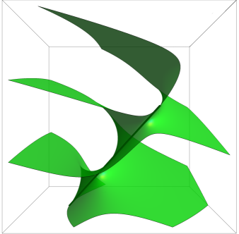
Figure 1. Local structure of the zero set $u^{-1}(0)$ when $f$ has regular zeros.

∎

Remark 3.2.

If $s>\frac{n+5+2l}{2}$ for some integer $l\geqslant 1$, one can conclude that $\frac{r^{\frac{n-1}{2}}}{2(2\pi)^{\frac{n-1}{2}}}u$ is close to $U$ in the $C^{l+1}(\mathbb{R}^{n})$ norm, so [EPS13, Theorem 3.1] then ensures that $\|\Phi_{k}-\mathrm{id}\|_{C^{l}(\mathbb{R}^{n})}<C/k$. This immediately yields asymptotic formulas for the area of each nodal component $\mathcal{S}_{k}$.

4. Proof of Theorem 1.3

Let us start by introducing some notation associated with the probabilistic setting described in Equation (1.2). We denote by $\mathbb{P}_{lm}$ the probability distribution of the random variable $a_{lm}$, which we are assuming to be a normal distribution of the form $\mathcal{N}(0,\sigma_{l}^{2})$. By Kolmogorov’s extension theorem, the associated probability measure in $\mathbb{R}^{\mathbb{N}}$ is the product measure that we will denote by $\mathbb{P}_{a}:=\prod_{{l}=0}^{\infty}\prod_{m=1}^{d_{l}}\mathbb{P}_{lm}$. The associated measures on the space of distributions on $\SS$ and on $\mathbb{R}^{n}$ are respectively given by the pushed forward measures $\mathbb{P}_{f}:=f_{*}\mathbb{P}_{a}$ and $\mathbb{P}:=u_{*}\mathbb{P}_{a}$, which we view as maps

$$f:\omega\in\Omega\backslash\Omega_{0}\mapsto\sum_{{l}=0}^{\infty}\sum_{m=1}^{d_{l}}i^{l}a_{{l}m}(\omega)\,Y_{lm}(\cdot)\in\mathcal{D}^{\prime}(\SS)\,,$$

and

$$u:\omega\in\Omega\backslash\Omega_{0}\mapsto(2\pi)^{\frac{n}{2}}\sum_{l=0}^{\infty}\sum_{m=1}^{d_{l}}a_{lm}(\omega)\,Y_{lm}\bigg{(}\frac{\cdot}{|\cdot|}\bigg{)}\,\frac{J_{l+\frac{n}{2}-1}(|\cdot|)}{|\cdot|^{\frac{n}{2}-1}}\in\mathcal{D}^{\prime}(\mathbb{R}^{n})\,,$$ (4.1)

where $\Omega_{0}\subset\Omega$ is a set of measure zero.

An important first observation is that, with the probability distribution we are considering, $f$ is an $H^{s}$-smooth function with probability 1:

Lemma 4.1.

The function $f$ is of class $H^{s}(\SS)$ almost surely.

Proof.

The hypothesis (1.3) implies that, for any $L>0$, the expected value of the finite sum is bounded by a uniform constant:

$$\mathbb{E}\left(\sum_{{l}=0}^{L}\sum_{m=1}^{d_{l}}a_{{l}m}^{2}({l}+1)^{2s}\right)=\sum_{{l}=0}^{L}{d_{l}}\sigma_{l}^{2}({l}+1)^{2s}<C\,.$$

The monotone convergence theorem then ensures that

$$\mathbb{E}\big{(}\|f\|_{H^{s}(\SS)}^{2}\big{)}=\mathbb{E}\bigg{(}\sum_{{l}=0}^{\infty}\sum_{m=1}^{d_{l}}a_{{l}m}^{2}({l}+1)^{2s}\bigg{)}<C\,,$$

which implies that $\mathbb{P}_{f}(H^{s}(\SS))=1$. ∎

The next result we need is that, again with probability 1, $f^{-1}(0)$ is a regular level set:

Lemma 4.2.

The zero set of $f$ is regular almost surely. Furthermore, if $n=2$, almost surely $f$ does not vanish.

Proof.

Let us consider the vector field on the sphere $h(\theta,\lambda):=\nabla_{\mathbb{S}}f_{\mathrm{R}}(\theta)-\lambda\nabla_{\mathbb{S}}f_{\mathrm{I}}(\theta)$ for $\lambda\in\mathbb{R}$. If we take local coordinates $(y_{1},\dots,y_{n-1})$ around a point $\theta\in\SS$, the components of $h$ in this local chart are given by

$$h_{j}(\theta,\lambda):=\sqrt{g^{jj}}\partial_{y_{j}}f_{\mathrm{R}}(\theta)-\lambda\sqrt{g^{jj}}\partial_{y_{j}}f_{\mathrm{I}}(\theta)$$ (4.2)

with $1\leqslant j\leqslant n-1$, as

$$\nabla_{\mathbb{S}}f_{a}=\sum_{i}{\partial_{y_{i}}f_{a}}\sqrt{g^{ii}}\mathbf{e}_{i}$$ (4.3)

where $\mathbf{e}_{i}$ is the unit vector in our coordinates. Recall that, by Lemma 4.1, $f\in C^{3}(\SS)$ almost surely.

In order to show that $(f_{\mathrm{R}},f_{\mathrm{I}},h)$ is a non-degenerate Gaussian vector field, we first analyze the probabilistic structure of $f$ and its derivatives, for which we need to compute the covariance matrix of ($f_{\mathrm{R}},f_{\mathrm{I}},\nabla_{\mathbb{S}}f_{\mathrm{R}},\nabla_{\mathbb{S}}f_{\mathrm{I}}$). We recall that a non-degenerate Gaussian vector field means that the determinant of its covariance matrix is positive definite everywhere.

First, the covariance between $f_{\mathrm{R}}$ (or derivatives of $f_{\mathrm{R}}$) and $f_{\mathrm{I}}$ (or derivatives of $f_{\mathrm{I}}$) is zero because they depend on different independent coefficients, even and odd $l$ respectively. Second, since the Gaussian coefficients have zero mean, the expected values of $f_{a}$ and $\nabla_{\mathbb{S}}f_{a}$ are zero, where $f_{a}$ denotes either $f_{\mathrm{R}}$ or $f_{\mathrm{I}}$. For the covariance kernel of $f_{a}$, notice that if $\theta,\theta^{\prime}\in\SS$, we have

$$\mathbb{E}\left(f_{a}(\theta)f_{a}(\theta^{\prime})\right)=\sum_{{l}=0,\text{parity}=a}^{\infty}\sigma_{l}^{2}c_{ln}P_{{l}n}(\theta\cdot\theta^{\prime})\,,$$ (4.4)

where $P_{{l}n}$ is the Legendre polynomial of degree ${l}$ in $n$ dimensions, $c_{ln}$ was defined in Equation (2.6) and the notation $\text{parity}=a$ means that the sum is restricted to even $l$ if $a=\text{R}$ and to odd $l$ if $a=\text{I}$. From the kernel Equation (4.4) we can deduce the variance of $f_{a}$,

$$\mathbb{E}\left(f_{a}(\theta)f_{a}(\theta)\right)=\sum_{{l}=0,\text{parity}=a}^{\infty}\sigma_{l}^{2}c_{ln}\in(0,+\infty)\,,$$

which is independent of $\theta$ and finite by our hypothesis on $\sigma_{l}$.

Let us now prove that $f_{a}$ and its derivatives are independent. Indeed, the covariance between the function and a derivative reads as

$$\mathbb{E}\left(f_{a}(\theta)\partial_{y_{i}}f_{a}(\theta)\right)=\left.\sum_{{l}=0,\text{parity}=a}^{\infty}\sigma_{l}^{2}c_{ln}P^{\prime}_{{l}n}(\theta\cdot\theta^{\prime})\theta\cdot\partial_{y^{\prime}_{i}}\theta^{\prime}\right|_{\theta^{\prime}=\theta}=0\,,$$

where we have used that $\theta$ is a point on the unit sphere and hence $\theta\cdot\theta=1$. We also claim that the derivatives are independent. To prove it, we assume that the vector fields $\{\partial_{y_{i}}\}$ are orthogonal, i.e., $g_{ij}=0$ if $1\leqslant i<j\leqslant n-1$, where $g_{ij}$ is the induced metric on $\SS$. This can be accomplished, for instance, by taking hyperspherical coordinates. If $g^{ij}$ denotes the inverse matrix of $g_{ij}$, we have

$$\mathbb{E}\left(\sqrt{g^{ii}}\partial_{y_{i}}f_{a}(\theta)\sqrt{g^{jj}}\partial_{y_{j}}f_{a}(\theta)\right)=$$

$$=\sqrt{g^{ii}}\sqrt{g^{jj}}\left.\sum_{{l}=0,\text{parity}=a}^{\infty}\sigma_{l}^{2}c_{ln}\left[P^{\prime}_{{l}n}(\theta\cdot\theta^{\prime})\partial_{y_{i}}\theta\cdot\partial_{y^{\prime}_{j}}\theta^{\prime}+P^{\prime\prime}_{{l}n}(\theta\cdot\theta^{\prime})\left(\partial_{y_{i}}\theta\cdot\theta^{\prime}\right)\left(\hskip 0.28453pt\theta\cdot\partial_{y^{\prime}_{j}}\theta^{\prime}\right)\right]\right|_{\theta=\theta^{\prime}}$$

$$=\sum_{{l}=0,\text{parity}=a}^{\infty}\sigma_{l}^{2}c_{ln}P^{\prime}_{{l}n}(1)(\partial_{y_{i}}\theta)^{2}\delta_{ij}\frac{1}{g_{ii}}=\delta_{ij}\sum_{{l}=0,\text{parity}=a}^{\infty}\sigma_{l}^{2}c_{ln}P^{\prime}_{{l}n}(1)$$ (4.5)

where in the second and third equalities we have used the orthogonality condition of the coordinate system and the definition of the metric

$$g_{ij}=\partial_{y_{i}}\theta\cdot\partial_{y_{j}}\theta\,.$$

As before, this covariance matrix is strictly positive definite, independent of the point and finite. The finiteness follows from the differential equation satisfied by $P_{{l}n}$,

$$\left(1-x^{2}\right)^{\frac{3-n}{2}}{\frac{d}{dx}}\left[\left(1-x^{2}\right)^{\frac{n-1}{2}}{\frac{dP_{{l}n}(x)}{dx}}\right]+{l}({l}+n-2)P_{{l}n}(x)=0\,,$$

which allows us to compute $P^{\prime}_{{l}n}(1)=\frac{{l}({l}+n-2)}{n-1}.$ Using Equation (4.3) we conclude that the covariance matrix of ($f_{\mathrm{R}},f_{\mathrm{I}},\nabla_{\mathbb{S}}f_{\mathrm{R}},\nabla_{\mathbb{S}}f_{\mathrm{I}}$) is diagonal and positive definite.

We are now ready to prove that $(f_{\mathrm{R}},f_{\mathrm{I}},h)$ is a non-degenerate Gaussian vector field. To see this, first notice that the computations above imply that $f_{\mathrm{R}}$, $f_{\mathrm{I}}$ and their derivatives are independent as they are uncorrelated (i.e., their covariance matrix vanishes), which ensures that the Gaussian vector field $(f_{\mathrm{R}},f_{\mathrm{I}},h)$ has zero mean (as linear combinations of independent Gaussian random variables are still Gaussian, our field is Gaussian). Also, the local expression (4.2) also ensures that

$$\mathbb{E}\left(f_{\mathrm{R}}(x)h(x)\right)=\mathbb{E}\left(f_{\mathrm{I}}(x)h(x)\right)=0\,.$$

By Equation (4.5),

$$\mathbb{E}\left(h_{i}(\theta,\lambda)h_{j}(\theta,\lambda)\right) =\delta_{ij}\left(\sum_{{l}=0,\text{parity}=\text{ even}}^{\infty}\sigma_{l}^{2}c_{ln}P^{\prime}_{{l}n}(1)+\lambda^{2}\sum_{{l}=0,\text{parity}=\text{ odd}}^{\infty}\sigma_{l}^{2}c_{ln}P^{\prime}_{{l}n}(1)\right)$$

$$=:\delta_{ij}(\sigma_{\mathrm{R}}^{2}+\lambda^{2}\sigma_{\mathrm{I}}^{2}).$$

We can now use suitable generalizations of Bulinskaya’s lemma [AW09, Proposition 6.11] to conclude that

$$\mathbb{P}_{f}(\{\exists\,\theta,\lambda:f(\theta)=0,\;h(\theta,\lambda)=0\})=0\,.$$

Indeed, $(f_{\mathrm{R}},f_{\mathrm{I}},h)$ is a non-degenerate Gaussian vector field going from an $n$-dimensional space to $\mathbb{R}^{n+1}$ and it is $C^{2}(\SS)$ almost surely. As the covariance matrix determinant, $\det\Sigma(\lambda)$, attains its minimum value at $\lambda=0$, independent of $\theta$ and strictly positive, the density of $(f_{\mathrm{R}},f_{\mathrm{I}},h)$ at zero is bounded for all values of $\theta,\lambda$, i.e.,

$$\rho(x,\lambda)={\displaystyle{\frac{\exp\left(-{\frac{1}{2}}x^{\mathrm{T}}{{\Sigma(\lambda)}}^{-1}x\right)}{\sqrt{(2\pi)^{n+1}|{\det{\Sigma(\lambda)}}|}}}}\leq\rho(0,0)<\infty.$$

This shows that the zero set of $f$ is regular almost surely as $\nabla_{\mathbb{S}}f_{\mathrm{R}}$ and $\nabla_{\mathbb{S}}f_{\mathrm{I}}$ are linearly independent at $f^{-1}(0)$.

When $n=2$, the same argument applied to the Gaussian vector field $(f_{\mathrm{R}},f_{\mathrm{I}})$ shows that

$$\mathbb{P}_{f}(\{\exists\,\theta:f(\theta)=0\})=0\,,$$

so with probability 1 the function $f$ does not vanish, and the lemma follows. ∎

In the next lemma we compute the probability that $f$ does not vanish and that $f$ has a nonempty regular zero set:

Lemma 4.3.

The probability that the function $f$ does not vanish on $\SS$ is $p_{2}:=1$ if $n=2$ and $p_{n}\in(0,1)$ if $n\geqslant 3$. Moreover, with probability $1-p_{n}$ the zero set $f^{-1}(0)$ is regular and nonempty.

Proof.

Given any function $f_{0}\in H^{s}(\SS)$, whose coefficients for the expansion in spherical harmonics we will denote by $a_{lm}^{0}$, and any $\epsilon>0$, we claim that

$$\mathbb{P}_{f}\big{(}\{\|f-f_{0}\|_{H^{s}(\SS)}<\epsilon\}\big{)}>0\,.$$ (4.6)

To prove this, we start by noting that we can take some $L$, depending on $\epsilon$, such that

$$\mathbb{P}_{a}\left(\sum_{{l}=L}^{\infty}\sum_{m=1}^{d_{l}}|a_{lm}-a^{0}_{{l}m}|^{2}({l}+1)^{2s}<\frac{\epsilon}{2}\right)>0\,,$$

which is obvious because $f_{0}\in H^{s}(\SS)$ and $f$ is in $H^{s}(\SS)$ almost surely by Lemma 4.1. Equation (4.6) then follows because

$$\mathbb{P}_{f}\big{(}\{\|f-f_{0}\|_{H^{s}(\SS)}<\epsilon\}\big{)}\geqslant\\ \mathbb{P}_{a}\left(\sum_{{l}=L}^{\infty}\sum_{m=1}^{d_{l}}|a_{lm}-a^{0}_{{l}m}|^{2}({l}+1)^{2s}<\frac{\epsilon}{2}\right)\,\mathbb{P}_{a}\left(\sum_{{l}=1}^{L}\sum_{m=1}^{d_{l}}|a_{lm}-a^{0}_{{l}m}|^{2}({l}+1)^{2s}<\frac{\epsilon}{2}\right)>0\,.$$

For all $n\geqslant 2$, it then suffices to take $f_{0}:=1$ to conclude that

$$p_{n}:=\mathbb{P}_{f}(\{f>0\})>0\,;$$

indeed, by Lemma 4.2 one knows that $p_{2}=1$. Likewise, when $n\geqslant 3$, one can take any smooth function $f_{0}$ whose zero set is regular and nonempty to conclude, by the implicit function theorem, that

$$1-p_{n}=\mathbb{P}_{f}(\{\min_{\SS}|f|=0\})>0\,.$$

Notice that this argument does not work when $n=2$ because, as $f$ is complex-valued, the rank of $\nabla f_{0}$ on $f_{0}^{-1}(0)$ must be 2 to apply the implicit function theorem. Finally, by Lemma 4.2, the nodal set is regular almost surely, so the lemma follows. ∎

We are now ready to complete the proof of Theorem 1.3. Lemma 4.1 ensures that $f\in H^{s}(\SS)$ almost surely. Furthermore, by Lemma 4.3, with probability $p_{n}$, $f$ does not vanish, so in this case Theorem 3.1 ensures that the nodal set of $u$ has $R/\pi+o(R)$ components diffeomorphic to $\SS$ contained in $B_{R}$ and only $O(1)$ components that are not diffeomorphic to $\SS$. Also by Lemma 4.3, with probability $1-p_{n}$ the zero set $f^{-1}(0)$ is regular and nonempty, so Theorem 3.1 ensures that $N_{u}(R)=O(1)$. The theorem is then proved.

5. Proof of Theorem 1.6

Let us denote by $\mu$ the probability measure on $\mathbb{R}^{\mathbb{N}}$ defined by the random variables $a_{lm}$, which we now assume to be absolutely continuous with respect to the Lebesgue measure for $l<l_{0}$ and Gaussian distributions $\mathcal{N}(M_{lm},\sigma_{lm}^{2})$ for $l\geqslant l_{0}$. We denote by $\mathbb{P}_{a}^{0}$ and $\mathbb{P}_{a}$ the probability measures defined by random variables $a_{lm}\sim\mathcal{N}(0,1)$ and $a_{lm}\sim\mathcal{N}(0,\sigma_{l}^{2})$ as in Theorem 1.3, respectively.

To prove the theorem it is enough to show that in the first (respectively, second) case, the measures $\mu$ and $\mathbb{P}_{a}^{0}$ (respectively, $\mathbb{P}_{a}$) are mutually absolutely continuous. Kakutani’s dichotomy theorem, Proposition 2.21 in [DPZ14], ensures that, in the first case, these measures are mutually absolutely continuous if and only if the Radon–Nikodym derivative of the measures satisfies

$$\prod_{{l}=0}^{\infty}\prod_{m=1}^{d_{l}}\int_{-\infty}^{\infty}\bigg{(}\frac{d\mu_{lm}}{d\mathbb{P}_{a}^{0}}\bigg{)}^{1/2}\,d\mathbb{P}_{a}^{0}>0\,$$ (5.1)

(being always $\leq 1$). Since, for $l\geqslant l_{0}$,

$$\frac{d\mu_{lm}}{d\mathbb{P}_{a}^{0}}(x)=\frac{1}{\sigma_{lm}}e^{\frac{x^{2}}{2}-\frac{(x-M_{lm})^{2}}{2\sigma_{lm}^{2}}}\,,$$

one has

$$\int_{-\infty}^{\infty}\bigg{(}\frac{d\mu_{lm}}{d\mathbb{P}_{a}^{0}}\bigg{)}^{1/2}\,d\mathbb{P}_{a}^{0}=(2\pi\sigma_{lm})^{-1/2}\int_{-\infty}^{\infty}e^{-\frac{(x-M_{lm})^{2}}{4\sigma_{lm}^{2}}-\frac{x^{2}}{4}}\,dx=\bigg{(}\frac{2\sigma_{lm}}{1+\sigma_{lm}^{2}}\bigg{)}^{1/2}e^{-\frac{M_{lm}^{2}}{4+4\sigma_{lm}^{2}}}\,.$$

Minus the logarithm of the product (5.1) for $l\geqslant l_{0}$ is then given by the series

$$\mathcal{C}:=\sum_{{l}=l_{0}}^{\infty}\sum_{m=1}^{d_{l}}\frac{M_{lm}^{2}}{4+4\sigma_{lm}^{2}}+\frac{1}{2}\sum_{{l}=l_{0}}^{\infty}\sum_{m=1}^{d_{l}}\log\frac{1+\sigma_{lm}^{2}}{2\sigma_{lm}}\,.$$

As both terms are necessarily positive and using that a sequence $a_{n}\geqslant 1$ satisfies

$$\sum_{n=1}^{\infty}\log a_{n}<\infty\quad\text{if and only if}\quad\sum_{n=1}^{\infty}(a_{n}-1)<\infty\,,$$

we then infer that that necessary and sufficient condition for $\mathcal{C}<\infty$ (or, equivalently, for the product (5.1) to be nonzero) is that

$$\sum_{{l}=l_{0}}^{\infty}\sum_{m=0}^{d_{l}}\Bigg{[}\frac{M_{lm}^{2}}{\sigma_{{l}m}^{2}+1}+\frac{(\sigma_{{l}m}-1)^{2}}{\sigma_{{l}m}}\Bigg{]}<\infty\,.$$

Likewise, $\mu$ and $\mathbb{P}_{a}$ are mutually absolutely continuous if Equation (5.1) holds with $\mathbb{P}_{a}^{0}$ replaced by $\mathbb{P}_{a}$, which amounts to

$$\sum_{{l}=l_{0}}^{\infty}\sum_{m=0}^{d_{l}}\bigg{[}\frac{M_{lm}^{2}}{\sigma_{l}^{2}+\sigma_{lm}^{2}}+\frac{(\sigma_{{l}}-\sigma_{lm})^{2}}{\sigma_{{l}}\sigma_{lm}}\bigg{]}<\infty\,.$$

Theorem 1.6 then follows.

Remark 5.1.

When the probability measure $\mu$ is a general Gaussian measure (not necessarily a product), the Feldman–Hajek theorem [DPZ14, Theorem 2.25] characterizes when $\mu$ and $\mathbb{P}_{a}$ (or $\mathbb{P}_{a}^{0}$) are mutually absolutely continuous in terms of the mean and covariance operator of $\mu$. However, the resulting condition is not very illustrative and we have opted not to include it. Nevertheless, this means that the results can be extended to coefficients which are not necessarily independent. Also, similar considerations using Kakutani’s theorem can be applied to a product measure whose coefficients are not normal variables.

Appendix A The decay of $u$ in terms of the regularity of $f$

Standard arguments from the theory of distributions ensure that any polynomially bounded solution to the Helmholtz equation

$$\Delta u+u=0$$

on $\mathbb{R}^{n}$ can be written as the Fourier transform of a distribution supported on the unit sphere. The fundamental result that connects the decay of the solution $u$ with the regularity of its Fourier transform is a classical result of Herglotz [Hör15, Theorem 7.1.28]. In order to state it, let us denote by

$${\left|\kern-1.07639pt\left|\kern-1.07639pt\left|u\right|\kern-1.07639pt\right|\kern-1.07639pt\right|}^{2}:=\limsup_{R\to\infty}\frac{1}{R}\int_{B_{R}}u(x)^{2}\,dx$$

the Agmon–Hörmander seminorm of a function $u$ on $\mathbb{R}^{n}$.

Theorem A.1 (Herglotz).

A solution to the Helmholtz equation satisfies the decay condition

$${\left|\kern-1.07639pt\left|\kern-1.07639pt\left|u\right|\kern-1.07639pt\right|\kern-1.07639pt\right|}<\infty$$

if and only if there is a function $f\in L^{2}(\SS)$ such that

$$u=\widehat{f\,dS}\,.$$ (A.1)

Furthermore, this decay estimate is sharp in the sense that there is a universal constant such that

$$\frac{1}{C}{\left|\kern-1.07639pt\left|\kern-1.07639pt\left|u\right|\kern-1.07639pt\right|\kern-1.07639pt\right|}\leqslant\|f\|_{L^{2}(\SS)}\leqslant C{\left|\kern-1.07639pt\left|\kern-1.07639pt\left|u\right|\kern-1.07639pt\right|\kern-1.07639pt\right|}\,.$$

An immediate consequence of this result is that the derivatives of any function of the form Equation (A.1) with $f\in L^{2}(\SS)$ have the same decay at infinity. Indeed, for any k,

$${\left|\kern-1.07639pt\left|\kern-1.07639pt\left|\nabla^{k}u\right|\kern-1.07639pt\right|\kern-1.07639pt\right|}\leqslant C\|\xi^{k}f\|_{L^{2}(\SS)}\leqslant C\|f\|_{L^{2}(\SS)}\,,$$ (A.2)

and in general this is obviously sharp because $\Delta u=-u$.

However, it is not hard to see that higher regularity of $f$ translates into higher decay rates of the angular derivatives of $u$. In order to state this result, let us denote by

$$\not{\nabla}u:=\nabla u-\frac{x\cdot\nabla u}{|x|^{2}}x$$

the angular part of the gradient and set $\langle x\rangle:=(1+|x|^{2})^{1/2}$.

Proposition A.2.

A solution to the Helmholtz equation satisfies the decay condition

$${\left|\kern-1.07639pt\left|\kern-1.07639pt\left|u\right|\kern-1.07639pt\right|\kern-1.07639pt\right|}_{k}:=\sum_{j=0}^{k}{\left|\kern-1.07639pt\left|\kern-1.07639pt\left|\langle x\rangle^{j}\,\not{\nabla}^{j}u\right|\kern-1.07639pt\right|\kern-1.07639pt\right|}<\infty$$

if and only if there is a function $f\in H^{k}(\SS)$ such that

$$u=\widehat{f\,dS}\,.$$

Furthermore, this decay estimate is sharp in the sense that there is a universal constant such that

$$\frac{1}{C}{\left|\kern-1.07639pt\left|\kern-1.07639pt\left|u\right|\kern-1.07639pt\right|\kern-1.07639pt\right|}_{k}\leqslant\|f\|_{H^{k}(\SS)}\leqslant C{\left|\kern-1.07639pt\left|\kern-1.07639pt\left|u\right|\kern-1.07639pt\right|\kern-1.07639pt\right|}_{k}\,.$$

Proof.

A simple integration by parts yields

$$\not{\nabla}^{j}u=\frac{1}{|x|^{j}}\widehat{\nabla_{\mathbb{S}}^{j}f\,dS}\,,$$

so the result follows from Herglotz’s theorem. ∎

Remark A.3.

Roughly speaking, Herglotz’s theorem asserts that a solution $u$ to the Helmholtz equation on $\mathbb{R}^{n}$ can decay at most as $|x|^{-\frac{n-1}{2}}$, on average, and that this sharp decay rate is attained if and only if $f$ is in $L^{2}(\SS)$. Furthermore, this proposition says that the $k^{\text{th}}$ angular derivatives of $u$ can decay at the faster rate $|x|^{-\frac{n-1}{2}-k}$, and that this sharp rate is attained in an $L^{2}$-averaged sense if and only if $f\in H^{k}(\SS)$.

The case when $f$ is of lower regularity than $L^{2}$, for instance $f\in H^{-k}(\SS)$ for a positive integer $k$, can be partly understood with a similar reasoning. In this case, one can write

$$f=\sum_{j=0}^{k}\mathcal{L}_{j}f_{j}$$

with $f_{j}\in L^{2}(\SS)$ and $\mathcal{L}_{j}$ a differential operator on $\SS$ of order $j$ with smooth coefficients. Furthermore,

$$\|f\|_{H^{-k}(\SS)}=\sum_{j=0}^{k}\|f_{j}\|_{L^{2}(\SS)}\,.$$

Therefore, integrating by parts in the distributional formula

$$u(x)=\int_{\SS}e^{ix\cdot\xi}\,f(\xi)\,dS(\xi)\,,$$

one easily obtains that

$$\frac{1}{R}\int_{B_{R}}\frac{u(x)^{2}}{1+|x|^{2k}}\,dx\leqslant C\|f\|_{H^{-k}(\SS)}^{2}\,.$$

However one should note that, contrary to what happens in the previous results of this Appendix, these are not the only solutions to the Helmholtz equation with this decay rate. This is evidenced, e.g., by the solutions whose Fourier transform is

$$\widehat{u}(\xi)=\delta^{(k)}(|\xi|-1)\,.$$

References

• [AH12] K. Atkinson and W. Han. Spherical harmonics and approximations on the unit sphere. Springer, New York, 2012.
• [AW09] J.M. Azais and M. Wschebor. Level Sets and Extrema of Random Processes and Fields. Wiley, New York, 2009.
• [BMW19] D. Beliaev, S. Muirhead, and I. Wigman. Mean conservation of nodal volume and connectivity measures for gaussian ensembles. arXiv preprint arXiv:1901.09000, 2019.
• [CS19] Y. Canzani and P. Sarnak. Topology and nesting of the zero set components of monochromatic random waves. Comm. Pure Appl. Math., 72:343–374, 2019.
• [CK92] D.L. Colton and R. Kress. Inverse Acoustic and Electromagnetic Scattering, Springer, Berlin, 1992.
• [DPZ14] G. Da Prato and J. Zabczyk. Stochastic equations in infinite dimensions. Cambridge University Press, Cambridge, 2014.
• [EPS13] A. Enciso and D. Peralta-Salas. Submanifolds that are level sets of solutions to a second-order elliptic PDE. Adv. Math., 249:204–249, 2013.
• [EPS15] A. Enciso and D. Peralta-Salas. Existence of knotted vortex tubes in steady Euler flows, Acta Math. 214:61–134, 2015.
• [FLL15] Y. Fyodorov, A. Lerario and E. Lundberg. On the number of connected components of random algebraic hypersurfaces, J. Geom. Phys., 95:1–20, 2015.
• [GW16] D. Gayet and J.-Y. Welschinger. Universal components of random nodal sets. Comm. Math. Phys., 347:777–797, 2016.
• [Hör15] L. Hörmander. The analysis of linear partial differential operators I. Reprint of the second edition, Springer, New York, 2015.
• [Kra14] I. Krasikov. Approximations for the Bessel and Airy functions with an explicit error term. LMS J. Comput. Math., 17:209–225, 2014.
• [KW18] P. Kurlberg and I. Wigman. Variation of the Nazarov-Sodin constant for random plane waves and arithmetic random waves. Adv. Math., 330:516–552, 2018.
• [NS09] F. Nazarov and M. Sodin. On the number of nodal domains of random spherical harmonics. Amer. J. Math., 131:1337–1357, 2009.
• [NS16] F. Nazarov and M. Sodin. Asymptotic laws for the spatial distribution and the number of connected components of zero sets of gaussian random functions. J. Math. Phys. Anal. Geom., 12:205–278, 2016.
• [RS79] M. Reed and B. Simon. Methods of Modern Mathematical Physics III. Scattering Theory. Academic Press, New York, 1979.
• [Riv19] A. Rivera. Expected number of nodal components for cut-off fractional Gaussian fields. J. Lond. Math. Soc., 99:629–652, 2019.
• [SW19] P. Sarnak and I. Wigman. Topologies of nodal sets of random band-limited functions. Comm. Pure Appl. Math., 72:275–342, 2019.