Ferromagnetic fluctuations in the Rashba-Hubbard model

Abstract

We study the occurrence and the origin of ferromagnetic fluctuations in the longitudinal spin susceptibility of the $t$-$t^{\prime}$-Rashba-Hubbard model on the square lattice. The combined effect of the second-neighbor hopping $t^{\prime}$ and the spin-orbit coupling leads to ferromagnetic fluctuations in a broad filling region. The spin-orbit coupling splits the energy bands, leading to two van Hove fillings, where the sheets of the Fermi surface change their topology. Between these two van Hove fillings the model shows ferromagnetic fluctuations. We find that the these ferromagnetic fluctuations originate from interband contributions to the spin susceptibility. These interband contributions only arise if there is one holelike and one electronlike Fermi surface, which is the case for fillings in between the two van Hove fillings. We discuss implications for experimental systems and propose a test on how to identify these types of ferromagnetic fluctuations in experiments.

I Introduction

Recent technological advances in atomic-scale synthesis have allowed to fabricate heterostructure interfaces with tailored electronic structures and symmetry properties Hwang et al. (2012). In these heterostructures it is possible, for example, to tune the degree of inversion-symmetry breaking and the strength of spin-orbit coupling by modulating the layer thickness or by applying electric fields Shimozawa et al. (2014); Mizukami et al. (2011); Caviglia et al. (2008); Sunko et al. (2017); Bhowal and Satpathy (2019); Bi et al. (2015). Many of these heterostructures exhibit emergent phenomena not found in the bulk constituents Reyren et al. (2007); Brinkman et al. (2007); Takahashi et al. (2001); Moetakef et al. (2012); Jackson and Stemmer (2013); Gibert et al. (2012); Suzuki (2015); Nichols et al. (2016); Mazzola et al. (2018). Particularly interesting is the emergence of ferromagnetism at interfaces between correlated materials Brinkman et al. (2007); Takahashi et al. (2001); Moetakef et al. (2012); Jackson and Stemmer (2013); Gibert et al. (2012); Suzuki (2015); Nichols et al. (2016); Mazzola et al. (2018), as this could be of potential use for spintronics applications. Interface ferromagnetism can arise both due to itinerant electrons, or due to localized spins at the interface. The former case most likely occurs at surfaces of the delafossite oxides PdCoO₂ and PdCrO₂ Mazzola et al. (2018), and at interfaces of GdTiO₃/SrTiO₃ Moetakef et al. (2012); Jackson and Stemmer (2013). In order to understand how interface ferromagnetism can emerge in these heterostructures, it is necessary to study the interplay of inversion-symmetry breaking, spin-orbit coupling, and correlation effects.

Motivated by these deliberations, we study in this article itinerant magnetic fluctuations in the Rashba-Hubbard model on the square lattice, which describes the salient features of interface electrons in a great number of heterostructures Laubach et al. (2014); Zhang et al. (2015); Brosco and Capone (2018); Ghadimi et al. (2019); bid and which, moreover, is relevant for many noncentrosymmetric materials with strong spin-orbit coupling Meza and Riera (2014); Yanase and Sigrist (2007, 2008); Yokoyama et al. (2007). Previously, we have studied this model in the context of superconductivity using the random phase approximation (RPA), and found that both spin-singlet and spin-triplet superconductivity can arise Greco and Schnyder (2018). Here, we want to investigate the itinerant magnetism and study the magnetic fluctuations as a function of electronic structure, on-site interaction $U$, and Rashba spin-orbit coupling (SOC). In particular, we want to focus on the longitudinal ferromagnetic (FM) fluctuations, which occur for fillings $n$ in between the two van Hove fillings, $n_{\textrm{vH${}_{2}$}}<n<n_{\textrm{vH${}_{1}$}}$. Our aim is to find the origin of these FM fluctuations and to show that they exist in a large region of parameter space.

We find that the longitudinal FM fluctuations originate from interband contributions to the spin susceptibility. These interband contributions are dominant if there is one holelike and one electronlike Fermi surface (FS), i.e., when the filling $n$ is in between $n_{\textrm{vH${}_{2}$}}$ and $n_{\textrm{vH${}_{1}$}}$. It follows from this insight, that longitudinal FM fluctuations occur quite commonly, i.e., in any Rashba system with one holelike and one electronlike Fermi surface. This is confirmed by our numerical calculations, which show that FM fluctuations are present whenever the filling is in between $n_{\textrm{vH${}_{2}$}}$ and $n_{\textrm{vH${}_{1}$}}$, independent of the magnitude of the second-neighbor hopping and SOC. The FM fluctuations survive also up to values of $U$ close to the magnetic instability, as obtained within the RPA. We note that the mechanism for FM fluctuations presented in this article is markedly different from Stoner ferromagnetism, which only occurs close to large maxima in the density of states (DOS) Rømer et al. (2015). As an experimental test to detect these type of FM fluctuations we propose to measure the ratio between the longitudinal and transversal susceptibilities, which shows pronounced features as a function of SOC and filling.

The remainder of this paper is organized as follows. In Sec. II we present briefly our model and theoretical framework. In Sec. III we study the itinerant fluctuations as a function of SOC and second-neighbor hopping $t^{\prime}$. The origin of the ferromagnetic and antiferromagnetic fluctuations is discussed in Sec. IV. In Sec. V we propose possible experimental tests for detecting the predicted ferromagnetic fluctuations. Section VI contains discussions and conclusions. In Appendices A and B we provide the main mathematical aspects of the present calculation.

II Model and theoretical scheme

The one-band Rashba-Hubbard model on the two-dimensional square lattice is defined by

$$H=\sum_{\bf k}{\psi}^{\dagger}_{\bf k}\hat{h}({\bf k})\psi^{\ }_{{\bf k}}+U\sum_{{\bf k},{\bf k^{\prime}},{\bf q}}c^{\dagger}_{{\bf k}\uparrow}c^{\ }_{{\bf k}+{\bf q}\uparrow}c^{\dagger}_{{\bf k^{\prime}}\downarrow}c^{\ }_{{\bf k^{\prime}}-{\bf q}\downarrow},$$ (1a)

where the single-particle Hamiltonian $$\hat{h}({\bf k})$$ is

$$\hat{h}({\bf k})=\left(\varepsilon_{\bf k}\tau_{0}+{\bf g}_{\bf k}\cdot\boldsymbol{\tau}\right).$$ (1b)

The band energy $\varepsilon_{\bf k}=-2t(\cos k_{x}+\cos k_{y})+4t^{\prime}\cos k_{x}\cos k_{y}-\mu$ contains both first- and second-neighbor hopping, $t$ and $t^{\prime}$, respectively, and $\mu$ is the chemical potential mis . The vector ${\bf g}_{\bf k}$ describes Rashba SOC with ${\bf g}_{\bf k}=V_{\textrm{so}}(\partial\varepsilon_{\bf k}/\partial k_{y},-\partial\varepsilon_{\bf k}/\partial k_{x},0)$ and the coupling constant $V_{\textrm{so}}$. $\boldsymbol{\tau}=(\tau_{1},\tau_{2},\tau_{3})^{T}$ are the three Pauli matrices and $\tau_{0}$ stands for the $2\times 2$ unit matrix. In Eq. (1a), $\psi_{\bf k}=(c_{{\bf k}\uparrow},c_{{\bf k}\downarrow})^{T}$ is a doublet of annihilation operators with wave vector ${\bf k}$ and $U$ is the on-site Coulomb repulsion. In the following, energies are given in units of $t$.

The presence of Rashba SOC splits the electronic dispersion $\varepsilon_{\bf k}$ of the single-particle Hamiltonian (1b) into negative- and positive-helicity bands with energies $E_{\bf k}^{1}=\varepsilon_{\bf k}-\left|{\bf g}_{\bf k}\right|$ and $E_{\bf k}^{2}=\varepsilon_{\bf k}+\left|{\bf g}_{\bf k}\right|$, respectively, see Fig. 1(b). These spin-split bands exhibit a helical spin polarization, which is described by the expectation value of the spin operator

$$\langle{\bf S}_{\bf k}\rangle_{i}=(-1)^{i}\frac{1}{2}\frac{{\bf g}_{\bf k}}{|{\bf g}_{\bf k}|},$$ (2)

where $i$ denotes the band index. The spin polarization is proportional to the normalized ${\bf g}$-vector ${\bf g}_{\bf k}/|{\bf g}_{\bf k}|$, and thus is purely within the $xy$ plane. Moreover, the spin polarization is of helical nature, i.e., to a good approximation perpendicular to the momentum (tangential to the Fermi surface).

In order to study the magnetic fluctuations of Hamiltonian (1), we compute the spin susceptibility $\hat{\chi}({\bf q},i\omega_{l})$ using RPA, which is known to provide a reasonable description of the essential physics, at least within weak coupling Yanase and Sigrist (2007, 2008); Yokoyama et al. (2007); Greco and Schnyder (2018). Within the RPA, the dressed spin susceptibility is given by

$$\hat{\chi}({\bf q},i\omega_{l})=\left[I-\hat{\chi}^{(0)}({\bf q},i\omega_{l})\hat{U}\right]^{-1}\hat{\chi}^{(0)}({\bf q},i\omega_{l}),$$ (3)

where $\hat{\chi}^{(0)}$ is the bare spin susceptibility. Here, $\hat{\chi}$, $\hat{\chi}^{(0)}$, and $\hat{U}$ are $4\times 4$ matrices containing the sixteen components of $\chi_{\sigma_{1}\sigma_{2}\sigma_{3}\sigma_{4}}$, $\chi^{(0)}_{\sigma_{1}\sigma_{2}\sigma_{3}\sigma_{4}}$, and $U$, respectively. The longitudinal and transversal susceptibilities can be computed in terms of the matrix elements $\chi_{\sigma_{1}\sigma_{2}\sigma_{3}\sigma_{4}}$ as

$$\chi_{\textrm{long}}({\bf q},i\omega_{l})=\chi_{\uparrow\uparrow\uparrow\uparrow}({\bf q},i\omega_{l})-\chi_{\uparrow\downarrow\downarrow\uparrow}({\bf q},i\omega_{l}),$$ (4a)

and

$$\chi_{\textrm{trans}}({\bf q},i\omega_{l})=\chi_{\uparrow\uparrow\downarrow\downarrow}({\bf q},i\omega_{l}),$$ (4b)

respectively. More details on the derivation of the dressed spin susceptibility (3) are given in Appendix A.

III Spin fluctuations of Rashba-Hubbard model

To set the stage, we first recall some properties of the spin fluctuations in the square-lattice Hubbard model without SOC but finite $t^{\prime}$, corresponding to $V_{\textrm{so}}=0$ in Eq. (1). In the absence of SOC, full $SU(2)$ spin-rotation symmetry is preserved in the paramagnetic phase, and hence the longitudinal and transversal spin susceptibilities are equal, i.e., $\chi_{\textrm{long}}=\chi_{\textrm{trans}}$. As has been shown in numerous works Kamogawa et al. (2019); Rømer et al. (2015, 2019); Fleck et al. (1997), the spin fluctuations are in this case mostly of (incommensurate) AFM nature. Only very close to the van-Hove filling $n_{\textrm{vH}}$ there occur ferromagnetic fluctuations, which diminish quickly for fillings away from $n_{\textrm{vH}}$. These FM fluctuations can be understood as resulting from Stoner ferromagnetism Rømer et al. (2015); Kamogawa et al. (2019), which occurs for fillings close to a large asymmetric maximum in the DOS. Indeed, for finite $t^{\prime}$, the maximum in the DOS at the van-Hove filling $n_{\textrm{vH}}$ is always asymmetric [see dashed line in Fig. 1(a)], such that the Stoner criterion for ferromagnetism can be satisfied. We note, however, that for vanishing $t^{\prime}$ the DOS is symmetric, such that the Stoner criterion cannot be fulfilled. Hence, for $t^{\prime}=0$ the fluctuations are AFM also close to the van-Hove filling, due to perfect nesting of the Fermi surface.

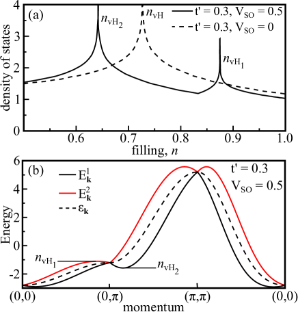
Figure 1: (a) Density of states versus filling $n$ for $t^{\prime}=0.3$, with $V_{\textrm{so}}=0$ (dashed line) and $V_{\textrm{so}}=0.5$ (solid line). (b) Band dispersions for $t^{\prime}=0.3$, with $V_{\textrm{so}}=0$ (dashed line) and $V_{\textrm{so}}=0.5$ (solid lines).

For finite Rashba SOC ($V_{\textrm{so}}\neq 0$) the situation changes drastically. First of all, Rashba SOC lifts the spin degeneracy of the bands, thereby splitting the van-Hove singularity into two divergences that occur at the fillings $n_{\textrm{vH${}_{1}$}}$ and $n_{\textrm{vH${}_{2}$}}$, see solid lines in Fig. 1. These two van-Hove singularities originate from saddle points in the dispersion at $(0,\pi-\delta)$, $(\delta,\pi)$, and symmetry related points. At these saddle points the gradient of the dispersion vanishes, causing logarithmic divergences in the DOS. Importantly, the topology of the Fermi surfaces changes as the filling $n$ crosses the two van-Hove fillings: For $n>n_{\textrm{vH${}_{1}$}}$ the two Fermi surfaces are hole-like and centered arount $(\pi,\pi)$, see Figs. 2(c) and 2(d). For $n_{\textrm{vH${}_{2}$}}<n<n_{\textrm{vH${}_{1}$}}$, on the other hand, one Fermi surface is electron-like, while the other his hole-like [Figs. 2(a) and 2(b)]. For $n<n_{\textrm{vH${}_{2}$}}$, both Fermi surfaces are electron-like and centered around $(0,0)$.

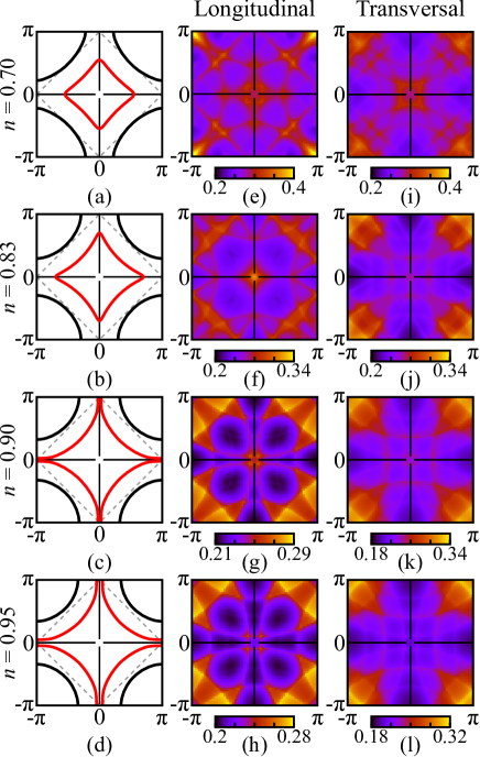
Figure 2: (a)-(d) Fermi surface topology for four different fillings. The dashed lines indicate the AFM zone boundary. (e)-(l) Color maps of the bare static susceptibilities as a function of modulation vector ${\bf q}$ for each of the four fillings. The second and third columns show the longitudinal and transversal static susceptibilities, ${\chi}^{(0)}_{\textrm{long}}({\bf q})$ and ${\chi}^{(0)}_{\textrm{trans}}({\bf q})$, respectively. Here, we set the temperature to $T=0.01$, and choose $t^{\prime}=0.3$ and $V_{\textrm{so}}=0.5$, for which the two van Hove singularities are located at $n_{\textrm{vH${}_{1}$}}=0.87$ and $n_{\textrm{vH${}_{2}$}}=0.65$.

As is known from a great many works on the Hubbard model Rømer et al. (2015); Scalapino et al. (1986); Hlubina (1999), the Fermi surface topology strongly influences the structure of the spin fluctuations. To uncover this dependence, we plot in Figs. 2(e)-2(l) the bare static susceptibility $\hat{\chi}^{(0)}({\bf q},\omega=0)\equiv\hat{\chi}^{(0)}({\bf q})$ as a function of modulation vector ${\bf q}$ for different fillings $n$. We find that for fillings with two hole-like Fermi surfaces ($n>n_{\textrm{vH${}_{1}$}}$), the dominant modulation vector of the longitudinal spin susceptibility ${\chi}^{(0)}_{\textrm{long}}({\bf q})$ is incommensurate AFM. For fillings with one electron-like and one hole-like Fermi surface ($n_{\textrm{vH${}_{2}$}}<n<n_{\textrm{vH${}_{1}$}}$), however, the longitudinal spin fluctuations are mostly FM [see Fig. 2(f)]. Finally, for fillings with two electron-like Fermi surfaces ($n<n_{\textrm{vH${}_{2}$}}$), the longitudinal spin fluctuations are dominantly AFM (not shown). The transversal spin susceptibility ${\chi}^{(0)}_{\textrm{trans}}({\bf q})$, in contrast to the longitudinal one, shows (incommensurate) AFM fluctuations for almost all fillings $n$.

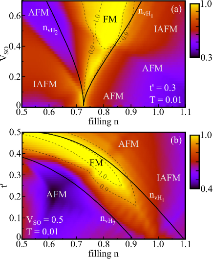
Figure 3: Relative intensity of the FM fluctuations compared to the incommensurate AFM fluctuations in the longitudinal susceptibility, ${\chi}^{(0)}_{\textrm{long}}({\bf q}={\bf 0})/{\chi}^{(0)}_{\textrm{long}}(\tilde{\bf q})$, as a function of filling $n$, Rashba SOC $V_{\textrm{so}}$ [panel (a)], and second neighbor hopping $t^{\prime}$ [panel (b)]. The solid lines represent the two van Hove fillings $n_{\textrm{vH${}_{1}$}}$ and $n_{\textrm{vH${}_{2}$}}$. IAFM stands for incommensurate AFM.

These findings are independent of the particular values of $t^{\prime}$ and $V_{\textrm{so}}$, as shown in Fig. 3. Here, we present the relative intensities of the FM fluctuations compared to the (incommensurate) AFM fluctuations in the longitudinal susceptibility. I.e., we plot ${\chi}^{(0)}_{\textrm{long}}({\bf q}={\bf 0})/{\chi}^{(0)}_{\textrm{long}}(\tilde{\bf q})$ where $\tilde{\bf q}$ is the location of the maximum of ${\chi}^{(0)}_{\textrm{long}}$. Inside the contour labeled “1” the maximum of ${\chi}^{(0)}_{\textrm{long}}$ is at the FM vector $\tilde{\bf q}=0$, while outside this contour, the maximum is at some (incommensurate) AFM vector, i.e., (close to) at $\tilde{\bf q}=(\pi,\pi)$. In Fig. 3(a) we plot the ratio ${\chi}^{(0)}_{\textrm{long}}({\bf q}={\bf 0})/{\chi}^{(0)}_{\textrm{long}}(\tilde{\bf q})$ as a function of $V_{\textrm{so}}$ and filling $n$ with fixed $t^{\prime}=0.3$, while in Fig. 3(b) it is shown as a function of $t^{\prime}$ and filling $n$ with fixed $V_{\textrm{so}}=0.5$. We observe a broad region, marked in yellow, where dominant FM fluctuations occur. These regions are bounded by the two van Hove fillings $n_{\textrm{vH${}_{1}$}}$ and $n_{\textrm{vH${}_{2}$}}$ (black lines). The full width at half maximum of the FM peak in these regions is about $0.4$, corresponding to a correlation length of about fifteen lattice constants. In Fig. 3(a) we see that with decreasing $V_{\textrm{so}}$, the FM fluctuation region becomes narrower and narrower, and shrinks to a single point at $n_{\textrm{vH}}=n_{\textrm{vH${}_{1}$}}=n_{\textrm{vH${}_{2}$}}$ for $V_{\textrm{so}}=0$. From Fig. 3(b) we find that as $t^{\prime}$ is increased the FM fluctuations occur at lower fillings $n$. Moreover, the FM fluctuations become dominant only for $t^{\prime}$ larger than a certain onset value, i.e., for $t^{\prime}\gtrsim 0.2$.

We note that in the entire parameter space the spin fluctuations are either FM (peaked at ${\bf q}=0$), commensurate AFM (peaked at ${\bf q}=(\pi,\pi)$), or incommensurate AFM (peaked at $\tilde{\bf q}$, with $\tilde{\bf q}$ away from, but close to $(\pi,\pi)$). Hence, the transition from FM to (incommensurate) AFM does not occur smoothly via a continuous evolution of the modulation vector ${\bf q}$, but rather abruptly when the peak at $\tilde{\bf q}$ suddenly becomes larger than the one at ${\bf q}=0$.

So far, we have focused on the bare susceptibility $\hat{\chi}^{(0)}({\bf q})$. The spin fluctuations of the dressed spin susceptibility $\hat{\chi}({\bf q})$, Eq. (3), are shown in Fig. 4. For small and intermediate $U$ the structure of the spin fluctuations of $\hat{\chi}({\bf q})$ is almost identical to the spin fluctuations of $\hat{\chi}^{(0)}({\bf q})$. This is to be expected, since a purely onsite interaction cannot change the momentum dependence of the spin fluctuations. For low and high fillings, $n<n_{\textrm{vH${}_{2}$}}$ and $n>n_{\textrm{vH${}_{1}$}}$, both longitudinal and transversal susceptibilities show dominant incommensurate AFM fluctuations. In between the two van Hove fillings, $n_{\textrm{vH${}_{2}$}}<n<n_{\textrm{vH${}_{1}$}}$, the transversal susceptibility exhibits incommensurate AFM fluctuations, while the longitudinal one shows FM fluctuations. These findings do not depend on the particular values of $t^{\prime}$ and $V_{\textrm{so}}$. That is, the phase diagram of Fig. 3, which shows the boundaries between the different magnetic fluctuations, remains almost identical upon inclusion of a small or intermediate onsite interaction $U$. Increasing $U$ beyond intermediate values, the FM fluctuations rapidly decrease as the critical interaction $U_{\textrm{c}}\simeq 2.5$ is approached Greco and Schnyder (2018), see first row of Fig. 4. For strong interactions $U\sim U_{c}$ (incommensurate) AFM fluctuations dominate [see Fig. 4(c) and (f)], leading to AFM order with magnetic moments oriented in-plane.

Hence, we conclude that the magnetic fluctuations remain largely unchanged by onsite interactions $U$ of small and intermediate strength. In particular, the FM fluctuations are unaffected; they originate from finite $t^{\prime}$ and finite SOC, rather than the interaction $U$. Thus, in order to uncover the root of the FM and AFM fluctuations, it is sufficient to consider the bare susceptibility $\hat{\chi}^{(0)}({\bf q})$, whose form is known exactly, and which can be analyzed using analytical means. This is the purpose of the next section.

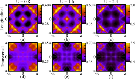
Figure 4: Color maps of the dressed static susceptibilities as a function of ${\bf q}$ for filling $n=0.83$ and different onsite interactions $U$ approaching the critical interaction $U_{c}$. The first and second rows show the longitudinal and transversal static susceptibilities, $\chi_{\textrm{long}}({\bf q})$ and $\chi_{\textrm{trans}}({\bf q})$, respectively. As in Fig. 2, we set $T=0.01$, $t^{\prime}=0.3$, and $V_{\textrm{so}}=0.5$, in which case $U_{c}\simeq 2.5$.

IV Origin of magnetic fluctuations

In this section we want to study the origin of the longitudinal FM and AFM fluctuations. To do so, we can focus on the bare susceptibility $\hat{\chi}^{(0)}_{\textrm{long}}$, as discussed above. We observe that $\hat{\chi}^{(0)}_{\textrm{long}}$ can be separated into interband and intraband parts. That is,

$$\chi^{(0)}_{\textrm{long}}({\bf q},i\omega_{l})=\chi^{(0),\textrm{intra}}_{\textrm{long}}({\bf q},i\omega_{l})+\chi^{(0),\textrm{inter}}_{\textrm{long}}({\bf q},i\omega_{l}),$$ (5)

where $\chi^{(0),\textrm{intra}}_{\textrm{long}}$ and $\chi^{(0),\textrm{inter}}_{\textrm{long}}$ are given in Appendix B. As discussed in Appendix B, the AFM fluctuations originate from the intraband term, while the FM fluctuations stem from the interband term, see Eqs. (15) to (18).

Let us first discuss the interband term, which is responsible for FM fluctuations. At the FM modulation vector ${\bf q}=(0,0)\equiv{\bf 0}$, the static interband susceptibility $\chi^{(0),\textrm{inter}}_{\textrm{long}}({\bf 0},\omega=0)$ takes the simple form

$$\chi^{(0),\textrm{inter}}_{\textrm{long}}({\bf 0})=\sum_{{\bf k}}\left[f(E_{\bf k}^{1})-f(E_{\bf k}^{2})\right]\frac{4|{g}_{\bf k}|}{4|{g}_{\bf k}|^{2}+\Gamma^{2}},\;\;$$ (6)

where $\Gamma$ is a small positive infinitesimal. Because $E_{\bf k}^{1}<E_{\bf k}^{2}$ and $f(z)$ is a decreasing function of $z$, we have $0\leq f(E^{1}_{\bf k})-f(E^{2}_{\bf k})\leq 1$ in the above expression. In the limit $\Gamma\to 0$, the summand in Eq. (6) exhibits a divergence at those ${\bf k}$ where ${\bf g}_{\bf k}=0$ and $f(E^{1}_{\bf k})-f(E^{2}_{\bf k})$ is nonzero. Since ${\bf g}_{\bf k}$ is inversion antisymmetric in ${\bf k}$, it vanishes at the four inversion-invariant momenta

$${\bf k}\in\{(0,0),(0,\pi),(\pi,0),(\pi,\pi)\}.$$ (7)

Hence, the second factor of Eq. (6) becomes larger and larger, and eventually diverges, as the above four momenta are approached. The Fermi factor $f(E_{\bf k}^{1})-f(E_{\bf k}^{2})$, on the other hand, also always vanishes at the four momenta of Eq. (7), where $E^{1}_{\bf k}=E^{2}_{\bf k}$. However, it can be nonzero in an arbitrarily small neighborhood around these points. This occurs near ${\bf k}\in\{(0,\pi),(\pi,0)\}$, when one Fermi surface is electron-like and the other one is hole-like. If the two Fermi surfaces are both electron-like (or hole-like), then the Fermi factor vanishes in a finite neighborhood around all four momenta of Eq. (7), thereby cancelling the divergence of the second factor in Eq. (6). These findings are illustrated in Figs. 5(a) and 5(b), which show the momentum dependence of the summand of Eq. (6). For filling $n=0.83$, corresponding to one electron-like and one hole-like Fermi surface, we observe that the summand diverges near ${\bf k}\in\{(0,\pi),(\pi,0)\}$, while for filling $n=0.95$, corresponding to two hole-like Fermi surfaces, the summand is finite for all ${\bf k}$. From this we deduce that strong FM fluctuations occur only for fillings in between the two van Hove fillings, i.e., when one Fermi surface is electron-like and the other one hole-like. As an aside, we note that close to the second van Hove singularity $n_{vH_{2}}$, i.e., for fillings $n_{vH_{2}}+\epsilon$ (with $\epsilon>0$) there is an additional Fermi pocket around $(0,\pi)$ and $(\pi,0)$. This additional Fermi pocket renders the Fermi factor $f(E^{1}_{\bf k})-f(E^{2}_{\bf k})$ zero in the neighborhood of $(0,\pi)$ and $(\pi,0)$. Therefore, the FM fluctuations, that originate from divergences of the second factor of Eq. (6) at $(0,\pi)$ and $(\pi,0)$, are suppressed for fillings close to $n_{vH_{2}}$, see Fig. 3.

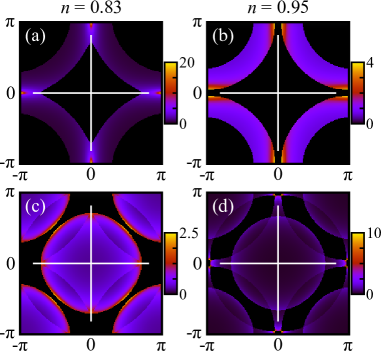
Figure 5: Momentum dependence of the summand of Eq. (6) [(a) and (b)] and of the summand of Eq. (8) [(c) and (d)]. In (a), (c) the filling is $n=0.83$, while in (b), (d) it is $n=0.95$. The parameters are $t^{\prime}=0.3$, $V_{\textrm{so}}=0.5$, and $\Gamma=0.05$. Note that four different color scales are used.

Next we study the intraband term of Eq. (5), which produces AFM fluctuations. At the AFM modulation vector ${\bf q}=(\pi,\pi)\equiv{\bf Q}$, the static intraband susceptibility $\chi^{(0),\textrm{intra}}_{\textrm{long}}({\bf Q},\omega=0)$ takes the simple form

$$\chi^{(0),\textrm{intra}}_{\textrm{long}}({\bf Q})=$$ (8)

$$\quad\sum_{\alpha=1,2}\sum_{{\bf k}}\left[f(E_{\bf k+Q}^{\alpha})-f(E_{\bf k}^{\alpha})\right]\frac{E_{\bf k+Q}^{\alpha}-E_{\bf k}^{\alpha}}{(E_{\bf k+Q}^{\alpha}-E_{\bf k}^{\alpha})^{2}+\Gamma^{2}}.$$

In the limit $\Gamma\to 0$, the summand in Eq. (8) has a divergence at those ${\bf k}$ where $E_{\bf k+Q}^{\alpha}=E_{\bf k}^{\alpha}$ and $f(E_{\bf k+Q}^{\alpha})-f(E_{\bf k}^{\alpha})$ is nonzero. The condition $E_{\bf k+Q}^{\alpha}=E_{\bf k}^{\alpha}$ is satisfied at the AFM zone boundary, indicated by the dashed lines in Figs. 2(a) - 2(d). This leads to a divergence of the second factor of Eq. (8), which is further enhanced near $(0,\pi)$ and $(\pi,0)$ by the saddle points in the dispersions of $E_{\bf k+Q}^{\alpha}$ and $E_{\bf k}^{\alpha}$. The Fermi factor $f(E_{\bf k+Q}^{\alpha})-f(E_{\bf k}^{\alpha})$, on the other hand, is nonzero near $(0,\pi)$ and $(\pi,0)$, only for the second band with fillings $n>n_{\textrm{vH${}_{1}$}}$ and for the first band with fillings $n<n_{\textrm{vH${}_{2}$}}$. For $n_{\textrm{vH${}_{2}$}}<n<n_{\textrm{vH${}_{1}$}}$, however, the Fermi factor always vanishes near $(0,\pi)$ and $(\pi,0)$, thus cancelling the divergence from the second factor in Eq. (8). These observations are illustrated by Figs. 5(c) and 5(d), which display the ${\bf k}$ dependence of the summand of Eq. (8). For $n=0.95$, corresponding to two hole-like Fermi surfaces, the summand show divergences near $(0,\pi)$ and $(\pi,0)$, while for $n=0.83$, corresponding to one hole-like and one electron-like Fermi surface, the summand does not show any divergences. We conclude that strong AFM fluctuations occur only for $n<n_{\textrm{vH${}_{2}$}}$ and $n>n_{\textrm{vH${}_{1}$}}$, but not in between the two van Hove fillings.

In this section we have focused on the bare susceptibility $\hat{\chi}^{(0)}_{\textrm{long}}$. But the above arguments also explain the origin of the FM and AFM fluctuations in the dressed susceptibility $\hat{\chi}^{\ }_{\textrm{long}}$, since an onsite interaction $U$ of small or intermediate strength does not alter the structure of the magnetic fluctuations (see discussion at the end of Sec. III). It is possible to generalize the given arguments in a straightforward manner to other Rashba systems on other types of lattices with correlations of weak or intermediate strength. Thus, we expect that FM fluctuations occur generically for a large class of Rashba systems with one electron-like and one hole-like Fermi surface.

V Experimental test to identify ferromagnetic fluctuations

In order to identify the discussed FM fluctuations in experiments, we propose to measure the ratio between the longitudinal and transversal static susceptibilities in the presence of a constant magnetic field, i.e., $R=\chi_{\textrm{long}}({\bf 0})/\chi_{\textrm{trans}}({\bf 0})$. In an experiment $\chi_{\textrm{long}}({\bf 0})$ is the response to a constant magnetic field perpendicular to the two-dimensional layer, while $\chi_{\textrm{trans}}({\bf 0})$ is the response to a field parallel to the layer. The ratio $R$ is expected to depend only weakly on material details. Moreover, $R$ shows pronounced features as a function of filling $n$ and Rashba SOC $V_{\textrm{so}}$, for which one could look for in experiments.

In Fig. 6(a) we present the results for $R$ versus filling $n$ for $V_{\textrm{so}}=0.5$, $t^{\prime}=0.3$, and different values of $U$. The broad peak larger than $1$ for fillings in between the two van Hove fillings, $n_{\textrm{vH${}_{2}$}}<n<n_{\textrm{vH${}_{1}$}}$, originates from the dominant FM fluctuations in $\chi_{\textrm{long}}$, as discussed above. As a function of onsite interaction $U$, the height of this peak remains nearly unchanged, for small and intermediate values of $U$. For strong $U$ close to $U_{c}\simeq 2.5$, the FM fluctuations rapidly vanish, as discussion in Sec. III.

In Fig. 6(b) we plot $R$ as a function of Rashba SOC $V_{\textrm{so}}$ for the filling $n=0.83$ , at which the FM fluctuations are strongest. The values of $U$ are the same as in panel (a). Interestingly, $R$ versus $V_{\textrm{so}}$ shows a pronounced step at $V_{\textrm{so}}^{\textrm{onset}}$, above which longitudinal FM fluctuations occur, cf. Fig. 3(a). We note that $V_{\textrm{so}}^{\textrm{onset}}$ corresponds to the SOC strength, for which the second van Hove singularity is located at the filling $n=0.83$, i.e., entering the yellow region in Fig. 3(a). As in Fig. 6(a), we find that $R$ above the step does not change much with increasing $U$, as long as $U$ is smaller than $U_{c}$.

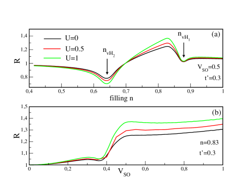
Figure 6: Ratio between the longitudinal and transversal static susceptibilities $R=\chi_{\textrm{long}}({\bf 0})/\chi_{\textrm{trans}}({\bf 0})$ as a function of (a) filling $n$ and (b) Rashba SOC $V_{\textrm{so}}$ for different values of $U$. In (a) the parameters are $t^{\prime}=0.3$ and $V_{\textrm{so}}=0.5$, while in (b) we set $t^{\prime}=0.3$ and $n=0.83$.

The discussed dependence of $R$ on filling $n$ and Rashba SOC $V_{\textrm{so}}$ could be measured in heterostructure interfaces. In these interfaces it is possible to control the filling by doping or gating Thiel et al. (2006). The Rashba SOC, on the other hand, can be tuned by applying electric fields or by modulating the layer thickness Caviglia et al. (2008); Shimozawa et al. (2014).

VI Discussions and conclusions

In summary, we have studied magnetic fluctuations of the $t$-$t^{\prime}$-Rashba-Hubbard model on the square lattice. The Rashba spin-orbit coupling of this model splits the bands and leads to two van Hove singularities. We have found that for fillings in between these two van Hove singularities, there exist dominant ferromagnetic fluctuations in the longitudinal susceptibility. Outside this filling region the magnetic fluctuations are (incommensurate) antiferromagnetic. The ferromagnetic fluctuations remain largely unchanged by onsite interactions $U$ of small and intermediate strength. They originate from interband contributions to the longitudinal susceptibility. These interband contributions only exist if there is a hole-like and an electron-like Fermi surface, which is the case for fillings in between the two van Hove singularities. Thus, the origin of these ferromagnetic fluctuations is different from the Stoner criterion for ferromagnetism, which is only satisfied close to large maxima in the density of states. As discussed in Sec. IV, these type of ferromagnetic fluctuations are expected to occur more generally, i.e., in any Rashba system with one electron-like and one hole-like Fermi surface.

We hope that our findings will stimulate experimentalists to look for two-dimensional materials or noncentrosymmetric systems that satisfy these conditions. In order to identify the ferromagnetic fluctuations in an experiment, we have proposed to measure the ratio between the longitudinal and transversal susceptibilities. This ratio is expected to depend only weakly on material details. It shows a pronounced step as a function of spin-orbit coupling and a broad peak as a function of filling, see Fig. 6.

To conclude, we mention several directions for future research. First of all, the reported ferromagnetic fluctuations could provide a pairing mechanism for unconventional superconductivity. We have recently reported some initial results concerning this in Ref. Greco and Schnyder (2018). It would be interesting to study in more detail the pairing symmetry of the superconductivity that is induced by the ferromagnetic fluctuations. Furthermore, it would be worthwhile to investigate the magnetic fluctuations of the Rashba-Hubbard model using more advanced techniques, such as FLEX Yanase et al. (2003) or fRG Metzner et al. (2012). Within the RPA we find that the ferromagnetic fluctuations do not lead to ferromagnetic order, since the antiferromagnetic fluctuations become stronger as $U$ approaches $U_{\textrm{c}}$. It would be interesting to know, whether this result is confirmed by more sophisticated methods.

Appendix A Spin susceptibility within the
random phase approximation

In this appendix, we give the precise definition of the dressed spin susceptibility. Within the RPA the dressed spin susceptibility $\chi_{\sigma_{1}\sigma_{2}\sigma_{3}\sigma_{4}}({\bf q},i\omega_{l})$ is given by Yanase and Sigrist (2007, 2008); Greco and Schnyder (2018)

$$\hat{\chi}({\bf q},i\omega_{l})=\left[I-\hat{\chi}^{(0)}({\bf q},i\omega_{l})\hat{U}\right]^{-1}\hat{\chi}^{(0)}({\bf q},i\omega_{l}),$$ (9)

where $\hat{\chi}^{(0)}$ is the bare spin susceptibility and $\hat{U}$ is the interaction matrix. Here, $\hat{\chi}^{(0)}$ and $\hat{\chi}$ are $4\times 4$ matrices with the matrix elements $\chi^{(0)}_{\sigma_{1}\sigma_{2}\sigma_{3}\sigma_{4}}$ and $\chi_{\sigma_{1}\sigma_{2}\sigma_{3}\sigma_{4}}$, respectively. The explicit form of the matrix $\hat{\chi}^{(0)}$ is given by

$$\hat{\chi}^{(0)}=\left(\begin{array}[]{llll}\chi^{(0)}_{\uparrow\uparrow\uparrow\uparrow}&\chi^{(0)}_{\uparrow\downarrow\uparrow\uparrow}&\chi^{(0)}_{\uparrow\uparrow\downarrow\uparrow}&\chi^{(0)}_{\uparrow\downarrow\downarrow\uparrow}\\ \chi^{(0)}_{\uparrow\uparrow\uparrow\downarrow}&\chi^{(0)}_{\uparrow\downarrow\uparrow\downarrow}&\chi^{(0)}_{\uparrow\uparrow\downarrow\downarrow}&\chi^{(0)}_{\uparrow\downarrow\downarrow\downarrow}\\ \chi^{(0)}_{\downarrow\uparrow\uparrow\uparrow}&\chi^{(0)}_{\downarrow\downarrow\uparrow\uparrow}&\chi^{(0)}_{\downarrow\uparrow\downarrow\uparrow}&\chi^{(0)}_{\downarrow\downarrow\downarrow\uparrow}\\ \chi^{(0)}_{\downarrow\uparrow\uparrow\downarrow}&\chi^{(0)}_{\downarrow\downarrow\uparrow\downarrow}&\chi^{(0)}_{\downarrow\uparrow\downarrow\downarrow}&\chi^{(0)}_{\downarrow\downarrow\downarrow\downarrow}\end{array}\right)\;,$$ (10)

and similarly for $\hat{\chi}$. The interaction matrix $\hat{U}$ is a $4\times 4$ antidiagonal matrix of the form

$$\hat{U}=\left(\begin{array}[]{llll}0&0&0&U\\ 0&0&-U&0\\ 0&-U&0&0\\ U&0&0&0\end{array}\right)\;.$$ (11)

In the above expressions, the bare susceptibility $\chi^{(0)}_{\sigma_{1}\sigma_{2}\sigma_{3}\sigma_{4}}({\bf q},i\omega_{l})$ is defined as the convolution of two Green’s functions

$$\chi^{(0)}_{\sigma_{1}\sigma_{2}\sigma_{3}\sigma_{4}}({\bf q},i\omega_{l})=$$

$$\qquad\sum_{{\bf k},i\nu_{n}}G^{(0)}_{\sigma_{1}\sigma_{2}}({\bf k},i\nu_{n})G^{(0)}_{\sigma_{3}\sigma_{4}}({\bf k}+{\bf q},i\nu_{n}+i\omega_{l}),\qquad$$ (12a)

with

$$G^{(0)}_{\sigma_{1}\sigma_{2}}({\bf k},i\nu_{n})=\left(\left[i\nu_{n}\sigma_{0}-\hat{h}({\bf k})\right]^{-1}\right)_{\sigma_{1}\sigma_{2}}$$ (12b)

the $2\times 2$ bare electronic Green’s function. Here, $\omega_{l}=2n\pi/\beta$ is the bosonic Matsubara frequency, while $\nu_{n}=(2n+1)\pi/\beta$ is the fermionic Matsubara frequency, with $\beta$ the inverse temperature.

Appendix B Simplified expressions for the longitudinal bare susceptibility

In this appendix, we derive simplified expressions for the longitudinal bare spin susceptibility $\chi^{(0)}_{\textrm{long}}$. First we show that $\chi^{(0)}_{\textrm{long}}$ can be split into intra- and interband contributions. For that purpose we note that the four components of the bare Green’s function, Eq. (12b), can be written as

$$G^{(0)}_{\uparrow\uparrow}({\bf k},i\nu_{l}) = G^{(0)}_{\downarrow\downarrow}({\bf k},i\nu_{l})=\frac{1/2}{i\nu_{l}-E_{\bf k}^{1}}+\frac{1/2}{i\nu_{l}-E_{\bf k}^{2}},$$ (13)

and

$$G^{(0)}_{\uparrow\downarrow}({\bf k},i\nu_{l}) = G^{*{(0)}}_{\uparrow\downarrow}({\bf k},i\nu_{l})=\frac{\hat{{V}}_{\bf k}/2}{i\nu_{l}-E_{\bf k}^{2}}-\frac{\hat{{V}}_{\bf k}/2}{i\nu_{l}-E_{\bf k}^{1}},$$ (14)

where ${\hat{V}}_{\bf k}=V_{\bf k}/|{V}_{\bf k}|$, with $V_{\bf k}={\bf g}_{\bf k}\cdot(1,i)$. Combining this with Eq. (12), we find that $\chi^{(0)}_{\textrm{long}}$ can be decomposed into an intraband and an interband part, i.e., $\chi^{(0)}_{\textrm{long}}=\chi^{(0),\textrm{intra}}_{\textrm{long}}+\chi^{(0),\textrm{inter}}_{\textrm{long}}$ with

$$\chi^{(0),\textrm{intra}}_{\textrm{long}}({\bf q},i\omega_{l})=\sum_{{\bf k}}\left[\frac{f(E_{\bf k+q}^{1})-f(E_{\bf k}^{1})}{E_{\bf k+q}^{1}-E_{\bf k}^{1}-i\omega_{l}}+\frac{f(E_{\bf k+q}^{2})-f(E_{\bf k}^{2})}{E_{\bf k+q}^{2}-E_{\bf k}^{2}-i\omega_{l}}\right]\frac{1}{2}(1-{\hat{\bf g}}_{\bf k}\cdot{\hat{\bf g}}_{\bf k+q}),$$ (15)

and

$$\chi^{(0),\textrm{inter}}_{\textrm{long}}({\bf q},i\omega_{l})=\sum_{{\bf k}}\left[\frac{f(E_{\bf k+q}^{1})-f(E_{\bf k}^{2})}{E_{\bf k+q}^{1}-E_{\bf k}^{2}-i\omega_{l}}+\frac{f(E_{\bf k+q}^{2})-f(E_{\bf k}^{1})}{E_{\bf k+q}^{2}-E_{\bf k}^{1}-i\omega_{l}}\right]\frac{1}{2}(1+{\hat{\bf g}}_{\bf k}\cdot{\hat{\bf g}}_{\bf k+q}),$$ (16)

respectively, where $\hat{\bf g}_{\bf k}={\bf g}_{\bf k}/|{\bf g}_{\bf k}|$ , $f(z)=(e^{\beta z}+1)^{-1}$ is the Fermi distribution function, and $\beta$ is the inverse temperature.

For AFM fluctuations with modulation vector ${\bf q}={\bf Q}(1+\delta)$ close to ${\bf Q}=(\pi,\pi)$, with $\delta\ll 1$, we find that ${\hat{\bf g}}_{\bf k}\cdot{\hat{\bf g}}_{{\bf k}+{\bf Q}(1+\delta)}=-1+\mathcal{O}[t^{\prime},\delta]$. Hence, the AFM fluctuations originate from the intraband term, while the interband term gives only a contribution of order $\mathcal{O}[t^{\prime},\delta]$. Thus, we have

$$\chi^{(0)}_{\textrm{long}}({\bf Q},i\omega_{l})\simeq\chi^{(0),\textrm{intra}}_{\textrm{long}}({\bf Q},i\omega_{l})=\sum_{{\bf k}}\left[\frac{f(E_{\bf k+Q}^{1})-f(E_{\bf k}^{1})}{E_{\bf k+Q}^{1}-E_{\bf k}^{1}-i\omega_{l}}+\frac{f(E_{\bf k+Q}^{2})-f(E_{\bf k}^{2})}{E_{\bf k+Q}^{2}-E_{\bf k}^{2}-i\omega_{l}}\right].$$ (17)

On the other hand, for FM fluctuations with ${\bf q}=(\delta,\delta)$ close to ${\bf q}={\bf 0}$, we have ${\hat{\bf g}}_{\bf k}\cdot{\hat{\bf g}}_{{\bf k}+(\delta,\delta)}=+1+\mathcal{O}[\delta^{2}]$. Therefore, the FM fluctuations stem from the interband term. That is, we find

$$\chi^{(0)}_{\textrm{long}}({\bf 0},i\omega_{l})=\chi^{(0),\textrm{inter}}_{\textrm{long}}({\bf 0},i\omega_{l})=\sum_{{\bf k}}\left[f(E_{\bf k}^{1})-f(E_{\bf k}^{2})\right]\left[\frac{4|{g}_{\bf k}|}{4|{g}_{\bf k}|^{2}+\omega_{l}^{2}}\right].$$ (18)

See the main text for a discussion of Eqs. (17) and (18).

References

- Hwang et al. (2012) H. Y. Hwang, Y. Iwasa, M. Kawasaki, B. Keimer, N. Nagaosa, and Y. Tokura, Nature Materials 11 (2012), URL https://doi.org/10.1038/nmat3223.
- Shimozawa et al. (2014) M. Shimozawa, S. K. Goh, R. Endo, R. Kobayashi, T. Watashige, Y. Mizukami, H. Ikeda, H. Shishido, Y. Yanase, T. Terashima, et al., Phys. Rev. Lett. 112, 156404 (2014), URL http://link.aps.org/doi/10.1103/PhysRevLett.112.156404.
- Mizukami et al. (2011) Y. Mizukami, H. Shishido, T. Shibauchi, M. Shimozawa, S. Yasumoto, D. Watanabe, M. Yamashita, H. Ikeda, T. Terashima, H. Kontani, et al., Nat Phys 7, 849 (2011), URL http://dx.doi.org/10.1038/nphys2112.
- Caviglia et al. (2008) A. D. Caviglia, S. Gariglio, N. Reyren, D. Jaccard, T. Schneider, M. Gabay, S. Thiel, G. Hammerl, J. Mannhart, and J. M. Triscone, Nature 456, 624 (2008), URL http://dx.doi.org/10.1038/nature07576.
- Sunko et al. (2017) V. Sunko, H. Rosner, P. Kushwaha, S. Khim, F. Mazzola, L. Bawden, O. J. Clark, J. M. Riley, D. Kasinathan, M. W. Haverkort, et al., Nature 549 (2017), URL https://doi.org/10.1038/nature23898.
- Bhowal and Satpathy (2019) S. Bhowal and S. Satpathy, npj Computational Materials 5 (2019), URL https://doi.org/10.1038/s41524-019-0198-8.
- Bi et al. (2015) F. Bi, M. Huang, H. Lee, C.-B. Eom, P. Irvin, and J. Levy, Applied Physics Letters 107, 082402 (2015), eprint https://doi.org/10.1063/1.4929430, URL https://doi.org/10.1063/1.4929430.
- Reyren et al. (2007) N. Reyren, S. Thiel, A. D. Caviglia, L. F. Kourkoutis, G. Hammerl, C. Richter, C. W. Schneider, T. Kopp, A.-S. Rüetschi, D. Jaccard, et al., Science 317, 1196 (2007), ISSN 0036-8075, eprint http://science.sciencemag.org/content/317/5842/1196.full.pdf, URL http://science.sciencemag.org/content/317/5842/1196.
- Brinkman et al. (2007) A. Brinkman, M. Huijben, M. van Zalk, J. Huijben, U. Zeitler, J. C. Maan, W. G. van der Wiel, G. Rijnders, D. H. A. Blank, and H. Hilgenkamp, Nature Materials 6 (2007), URL https://doi.org/10.1038/nmat1931.
- Takahashi et al. (2001) K. S. Takahashi, M. Kawasaki, and Y. Tokura, Applied Physics Letters 79, 1324 (2001), eprint https://doi.org/10.1063/1.1398331, URL https://doi.org/10.1063/1.1398331.
- Moetakef et al. (2012) P. Moetakef, J. R. Williams, D. G. Ouellette, A. P. Kajdos, D. Goldhaber-Gordon, S. J. Allen, and S. Stemmer, Phys. Rev. X 2, 021014 (2012), URL https://link.aps.org/doi/10.1103/PhysRevX.2.021014.
- Jackson and Stemmer (2013) C. A. Jackson and S. Stemmer, Phys. Rev. B 88, 180403 (2013), URL https://link.aps.org/doi/10.1103/PhysRevB.88.180403.
- Gibert et al. (2012) M. Gibert, P. Zubko, R. Scherwitzl, J. Ã?Ãiguez, and J.-M. Triscone, Nature Materials 11 (2012), URL https://doi.org/10.1038/nmat3224.
- Suzuki (2015) Y. Suzuki, APL Materials 3, 062402 (2015), eprint https://doi.org/10.1063/1.4921494, URL https://doi.org/10.1063/1.4921494.
- Nichols et al. (2016) J. Nichols, X. Gao, S. Lee, T. L. Meyer, J. W. Freeland, V. Lauter, D. Yi, J. Liu, D. Haskel, J. R. Petrie, et al., Nature Communications 7 (2016), URL https://doi.org/10.1038/ncomms12721.
- Mazzola et al. (2018) F. Mazzola, V. Sunko, S. Khim, H. Rosner, P. Kushwaha, O. J. Clark, L. Bawden, I. Marković, T. K. Kim, M. Hoesch, et al., Proceedings of the National Academy of Sciences 115, 12956 (2018), ISSN 0027-8424, eprint https://www.pnas.org/content/115/51/12956.full.pdf, URL https://www.pnas.org/content/115/51/12956.
- Laubach et al. (2014) M. Laubach, J. Reuther, R. Thomale, and S. Rachel, Phys. Rev. B 90, 165136 (2014), URL https://link.aps.org/doi/10.1103/PhysRevB.90.165136.
- Zhang et al. (2015) X. Zhang, W. Wu, G. Li, L. Wen, Q. Sun, and A.-C. Ji, New Journal of Physics 17, 073036 (2015), URL https://doi.org/10.1088%2F1367-2630%2F17%2F7%2F073036.
- Brosco and Capone (2018) V. Brosco and M. Capone, arXiv e-prints arXiv:1811.12034 (2018), eprint 1811.12034.
- Ghadimi et al. (2019) R. Ghadimi, M. Kargarian, and S. A. Jafari, Phys. Rev. B 99, 115122 (2019), URL https://link.aps.org/doi/10.1103/PhysRevB.99.115122.
- (21) M. Biderang et al., arXiv:1906.08130.
- Meza and Riera (2014) G. A. Meza and J. A. Riera, Phys. Rev. B 90, 085107 (2014), URL https://link.aps.org/doi/10.1103/PhysRevB.90.085107.
- Yanase and Sigrist (2007) Y. Yanase and M. Sigrist, Journal of the Physical Society of Japan 76, 043712 (2007), URL http://dx.doi.org/10.1143/JPSJ.76.043712.
- Yanase and Sigrist (2008) Y. Yanase and M. Sigrist, Journal of the Physical Society of Japan 77, 124711 (2008), eprint http://dx.doi.org/10.1143/JPSJ.77.124711, URL http://dx.doi.org/10.1143/JPSJ.77.124711.
- Yokoyama et al. (2007) T. Yokoyama, S. Onari, and Y. Tanaka, Phys. Rev. B 75, 172511 (2007), URL http://link.aps.org/doi/10.1103/PhysRevB.75.172511.
- Greco and Schnyder (2018) A. Greco and A. P. Schnyder, Phys. Rev. Lett. 120, 177002 (2018), URL https://link.aps.org/doi/10.1103/PhysRevLett.120.177002.
- Rømer et al. (2015) A. T. Rømer, A. Kreisel, I. Eremin, M. A. Malakhov, T. A. Maier, P. J. Hirschfeld, and B. M. Andersen, Phys. Rev. B 92, 104505 (2015), URL http://link.aps.org/doi/10.1103/PhysRevB.92.104505.
- (28) We have corrected the misprint of Ref. [Greco and Schnyder, 2018] where the second term of was written without the factor .
- Kamogawa et al. (2019) Y. Kamogawa, J. Nasu, and A. Koga, Phys. Rev. B 99, 235107 (2019), URL https://link.aps.org/doi/10.1103/PhysRevB.99.235107.
- Rømer et al. (2019) A. T. Rømer, T. A. Maier, A. Kreisel, I. Eremin, P. J. Hirschfeld, and B. M. Andersen, arXiv e-prints arXiv:1909.00627 (2019), eprint 1909.00627.
- Fleck et al. (1997) M. Fleck, A. M. Oleś, and L. Hedin, Phys. Rev. B 56, 3159 (1997), URL https://link.aps.org/doi/10.1103/PhysRevB.56.3159.
- Scalapino et al. (1986) D. J. Scalapino, E. Loh, and J. E. Hirsch, Phys. Rev. B 34, 8190 (1986), URL https://link.aps.org/doi/10.1103/PhysRevB.34.8190.
- Hlubina (1999) R. Hlubina, Phys. Rev. B 59, 9600 (1999), URL https://link.aps.org/doi/10.1103/PhysRevB.59.9600.
- Thiel et al. (2006) S. Thiel, G. Hammerl, A. Schmehl, C. W. Schneider, and J. Mannhart, Science 313, 1942 (2006), ISSN 0036-8075, eprint https://science.sciencemag.org/content/313/5795/1942.full.pdf, URL https://science.sciencemag.org/content/313/5795/1942.
- Yanase et al. (2003) Y. Yanase, T. Jujo, T. Nomura, H. Ikeda, T. Hotta, and K. Yamada, Physics Reports 387, 1 (2003), ISSN 0370-1573, URL http://www.sciencedirect.com/science/article/pii/S0370157303003235.
- Metzner et al. (2012) W. Metzner, M. Salmhofer, C. Honerkamp, V. Meden, and K. Schönhammer, Rev. Mod. Phys. 84, 299 (2012), URL https://link.aps.org/doi/10.1103/RevModPhys.84.299.