The headlight cloud in NGC 628:
An extreme giant molecular cloud in a typical galaxy disk

Abstract

Context. Cloud-scale surveys of molecular gas reveal the link between giant molecular cloud properties and star formation across a range of galactic environments. Cloud populations in galaxy disks are considered to be representative of the ‘normal’ star formation process, while galaxy centers tend to harbour denser gas that exhibits more extreme star formation. At high resolution, however, molecular clouds with exceptional gas properties and star formation activity may also be observed in normal disk environments. In this paper, we study the brightest cloud traced in CO(2$-$1) emission in the disk of nearby spiral galaxy NGC 628.

Aims. We characterize the properties of the molecular and ionized gas that is spatially coincident with an extremely bright H ii region in the context of the NGC 628 galactic environment. We investigate how feedback and large-scale processes influence the properties of the molecular gas in this region.

Methods. High resolution ALMA observations of CO(2$-$1) and CO(1$-$0) emission are used to characterize the mass and dynamical state of the “headlight” molecular cloud. The characteristics of this cloud are compared to the typical properties of molecular clouds in NGC 628. A simple large velocity gradient (LVG) analysis incorporating additional ALMA observations of ¹³CO(1$-$0), HCO⁺(1$-$0) and HCN(1$-$0) emission is used to constrain the beam-diluted density and temperature of the molecular gas. We analyze the MUSE spectrum using Starburst99 to characterize the young stellar population associated with the H ii region.

Results. The unusually bright headlight cloud is massive ($1-2\times 10^{7}$ $\mathrm{M_{\odot}}$), with a beam-diluted density of $n_{\rm H_{2}}=5\times 10^{4}$ cm^-3 based on LVG modeling. It has a low virial parameter, suggesting that the CO emission associated with this cloud may be overluminous due to heating by the H ii region. A young ($2-4$ Myr) stellar population with mass $3\times 10^{5}$ $\mathrm{M_{\odot}}$ is associated.

Conclusions. We argue that the headlight cloud is currently being destroyed by feedback from young massive stars. Due to the cloud’s large mass, this phase of the cloud’s evolution is long enough for the impact of feedback on the excitation of the gas to be observed. The high mass of the headlight cloud may be related to its location at a spiral co-rotation radius, where gas experiences reduced galactic shear compared to other regions of the disk, and receives a sustained inflow of gas that can promote the cloud’s mass growth.

1 Introduction

NGC 628 (M74) is a nearby ($d=9.6$ Mpc, Kreckel et al., 2017), almost face-on ($i\sim 9\degr$, Blanc et al., 2013), type SAc grand-design spiral galaxy with a stellar mass of $M_{\star}=1.5{-}2\times 10^{10}\,\mathrm{M_{\odot}}$ (Querejeta et al., 2015; Leroy et al., 2019) and moderate global star formation rate (SFR) of $\sim 2\,\mathrm{M_{\odot}}\,$yr^-1 (Sánchez et al., 2011). A well-known Messier object, NGC 628 is one of about ten galaxies that has been observed by nearly all recent major surveys of the interstellar gas and dust in nearby galaxies, including THINGS, HERACLES, SINGS, KINGFISH and EMPIRE (Walter et al., 2008; Leroy et al., 2009; Kennicutt et al., 2003, 2011; Bigiel et al., 2016). NGC 628 is likewise a popular target for observational studies of ionized gas and star formation in the local Universe, with existing wide-field WFPC3/ACS observations by the Hubble Space Telescope (HST) Legacy Extragalactic UV Survey (LEGUS) program (Calzetti et al., 2015) that enable a detailed characterisation of the population of stellar clusters and associations in NGC 628, as well as high-resolution, wide-field optical Integral Field Unit (IFU) imaging by the VENGA survey and CFHT/SITELLE (Blanc et al., 2013; Rousseau-Nepton et al., 2018).

Using the Multi Unit Spectroscopic Explorer (MUSE) optical IFU instrument on the Very Large Telescope (VLT), Kreckel et al. (2016, 2018) recently noted an extremely bright H ii region in the outer part of the galaxy (it is also visible, but uncommented on, in earlier H$\alpha$ mapping, e.g., Ferguson et al., 1998; Lelièvre & Roy, 2000). The source stands out as a bright, compact peak in the MUSE H$\alpha$ map. It is two orders of magnitude brighter than the mean H ii region in the galaxy population and twice as bright as the next most luminous source identified by Kreckel et al. (2018, see their Fig. 1). The H ii region has an equivalent radius of 142 pc, a velocity dispersion of 50 km s^-1, and an H$\alpha$ luminosity of $6.3\times 10^{39}\,$erg s^-1, which corresponds to a local SFR of $\sim 0.034$ $\mathrm{M_{\odot}}$ yr^-1, adopting the calibration of Kennicutt & Evans (2012). This bright H ii region is associated with bright, compact infrared emission in Spitzer and Herschel maps (e.g., see Aniano et al., 2012). It appears as the brightest spot in the galaxy in maps of WISE 12$\mu$m and 22$\mu$m emission (Leroy et al., 2019). The region thus exhibits the classic observational signatures of a large population of luminous young stars that are still associated with a large reservoir of interstellar gas and dust.

The association with gas is borne out by our new Atacama Large Millime- ter/submillimeter Array (ALMA) CO observations. We observed NGC 628 at $1^{\prime\prime}\sim 50$ pc resolution in CO(2$-$1) as part of a PHANGS-ALMA survey (PI: E. Schinnerer; co-PIs: A. Hughes, A. K. Leroy, A. Schruba, E. Rosolowsky). These NGC 628 CO maps have already appeared in Leroy et al. (2016), Sun et al. (2018), Kreckel et al. (2018), and Utomo et al. (2018). The ALMA data reveal an exceptionally bright CO peak spatially coincident with the H ii region (the association is particularly striking in Fig. 1 of Kreckel et al., 2018). While the source was visible in earlier CO maps (e.g., Wakker & Adler, 1995; Helfer et al., 2003; Leroy et al., 2009; Rebolledo et al., 2015), ALMA shows it to be stunningly compact and bright. This source is thus a compact, dust-enshrouded collection of many massive, young stars still associated with what appears to be the most massive molecular cloud in NGC 628. This object is even more remarkable because of its location at large galactocentric radius, which makes it distinct from the gas-rich, intensely star-forming regions that are commonly identified in galaxy centers.

A preliminary census of the disk environments in the PHANGS-ALMA galaxy sample suggests that this type of object is relatively rare, but not unique. To understand the internal and external factors that can influence the formation and evolution of such massive molecular clouds and their extraordinary H ii regions away from galaxy centers, a thorough examination of local physical conditions in the star-forming gas is essential. In this paper, we present the first such study, focusing on the CO-bright cloud in NGC 628 as a prototype. We name this object the headlight cloud, because it appears as a bright spot in an otherwise almost dark (unsaturated) map of the H$\alpha$ and CO emission.

Several factors make the headlight cloud the ideal candidate for this preliminary study. As noted above, NGC 628 is one of a limited (but growing) set of targets with information for a suite of millimetre and optical emission lines that can be used to constrain the physical properties of the molecular gas and the young stellar population. Relevant global galaxy properties (e.g. SFR) and the galaxy-scale gas dynamics in NGC 628 can be precisely characterized using the wealth of multi-wavelength imaging data. NGC 628 is also part of LEGUS (Calzetti et al., 2015). Studies using the LEGUS cluster catalog present a detailed quantitative overview of NGC 628’s cluster population, and the ability of NGC 628’s gas disk to form clusters and regulate their evolution (Adamo et al., 2017; Grasha et al., 2017; Ryon et al., 2017; Grasha et al., 2015). Nevertheless, the region hosting the headlight cloud lies just outside the coverage of the final multi-wavelength LEGUS mosaic.

Our goal in this paper is to measure the physical conditions in the molecular gas of the headlight cloud and to quantitatively describe the associated star formation activity. By comparing the measurements for the headlight cloud to the rest of the galaxy, we aim to build a picture of what may have prompted the growth of such a massive cloud and its extreme star formation event. The paper is structured as follows. Section 2 presents the observational data that we use. Section 3 describes the properties of the molecular gas. In Section 4, we discuss the stellar formation and feedback in the headlight cloud based on the MUSE data. In Section 5 we investigate the galactic environment of the headlight cloud. Section 6 discusses the results. Our conclusions are summarized in Section 7.

2 Observations

NGC 628 was observed with ALMA in Chile during ALMA’s Cycle 1 (ID: 2012.1.00650.S, PI: E. Schinnerer) and Cycle 2 (ID: 2013.1.00532.S, PI: E. Schinnerer). While the MUSE and CO (2$-$1) data have previously appeared elsewhere (see Sect. 1), the 3 mm line observations are presented here for the first time.

2.1 1 mm lines

The observational strategy, calibration and imaging of the interferometric data, array combination, and data product delivery of the PHANGS ALMA CO(2$-$1) data are described in a forthcoming dedicated PHANGS-ALMA survey paper (Leroy et al., in prep.). In Section 2.1.1 and 2.1.2, we briefly summarize the key steps for completeness. The present paper is the appropriate citation for the reduction of the PHANGS-ALMA total power data, which we present in detail in appendix A and summarize below. The strategy that we have used to reduce the CO(2$-$1) total power data for NGC 628 has been adopted as the basis for the PHANGS-ALMA total power processing pipeline.

2.1.1 Observations

ALMA Band 6 observations were obtained during Cycle 1 to image the emission of ¹²CO(2$-$1) (CO(2$-$1) hereafter), CS(5$-$4) and the 1 mm continuum. The covered frequency ranges in the source frame were 229.6-230.5 GHz and 231.0-232.8 GHz in the lower sideband (LSB), and 244.0-245.9 GHz and 246.7-246.8 GHz in the upper sideband (USB). The targeted field of view was a rectangular area of 240^′′$\times$175^′′ centered on the galaxy nucleus.

In order to recover all the spatial scales of the CO(2$-$1) emission, 12-m, 7-m, and Total Power observations were performed. On-The-Fly observations with three single-dish 12-m antennas delivered the Total Power. The off-source position was chosen at the offset $[240\mbox{${}^{\prime\prime}$},420\mbox{${}^{\prime\prime}$}]$ from the phase center located at $\alpha=01^{h}36^{m}41\aas@@fstack{s}72$, $\delta=+15\degr 46\arcmin 59\aas@@fstack{\prime\prime}3$ in the equatorial J2000 frame. Mosaics with a total of 149 and 95 pointings were observed with 27 to 38 antennas of the main 12-m array and with 7 to 9 antennas of the 7-m array, respectively. Eight, ten and twenty-four execution blocks were observed for the 12-m, 7-m, and Total Power arrays, respectively.

2.1.2 Reduction and Imaging

Table 1: Observational parameters of the ALMA observations.

Line	$\nu$	noise	Restored	$\Delta$vres	7m+
	GHz	K	beam	km s-1	TP
CS(5$-$4)	244.94	0.12a	1$\aas@@fstack{\prime\prime}$0 $\times$ 1$\aas@@fstack{\prime\prime}$0	5.0	no
12CO(2$-$1)	230.54	0.17a	1$\aas@@fstack{\prime\prime}$0 $\times$ 1$\aas@@fstack{\prime\prime}$0	2.5	yes
12CO(1$-$0)	115.27	0.12	1$\aas@@fstack{\prime\prime}$9 $\times$ 3$\aas@@fstack{\prime\prime}$1	6.0	yes
13CO(1$-$0)	110.20	0.03	2$\aas@@fstack{\prime\prime}$6 $\times$ 3$\aas@@fstack{\prime\prime}$5	6.0	yes
HNC(1$-$0)	90.66	1.2	2$\aas@@fstack{\prime\prime}$0 $\times$ 2$\aas@@fstack{\prime\prime}$1	15.0	no
HCO+(1$-$0)	89.19	1.1	2$\aas@@fstack{\prime\prime}$0 $\times$ 2$\aas@@fstack{\prime\prime}$2	15.0	no
HCN(1$-$0)	88.63	1.2	2$\aas@@fstack{\prime\prime}$1 $\times$ 2$\aas@@fstack{\prime\prime}$2	15.0	no

^aSensitivity measured in the region that was not fully covered by the interferometric data, which is where the headlight cloud is located. The sensitivity is 1.3 times better in the fully covered region.

The CO(2$-$1) observations were part of the pilot program for PHANGS-ALMA. Leroy et al. (in prep.) describe the selection, reduction, and imaging of the data in detail.

In summary, interferometric calibration followed the recipes provided in the ALMA reduction scripts. Visual inspection of the different calibration steps (bandpass, phase, amplitude, and flux) showed that the scripts yielded a satisfactory calibration. For these data, calibration was performed within the Common Astronomy Software Application (CASA), versions 4.2.2 and 4.2.1 for the 12-m and 7-m array observations, respectively. We used the task statwt on calibrated science data to ensure that the weights were estimated in a consistent way for 7-m and 12-m data reduced with different versions of CASA.

We imaged and post-processed the data using CASA version 5.4.0. The procedure is broadly as follows. We spectrally regrid all data onto a common velocity frame with channel width $\sim 2.5$ km s^-1. Then we combine and jointly image all 12-m and 7-m data together. We deconvolved the data in two stages. First, we carry out a multi-scale clean using the CASA task tclean. We used a broad clean mask and cleaned until the residual maps has a maximum signal-to-noise ratio of $4$. Then, we created a more restrictive clean mask and restarted the cleaning using a single scale clean at the highest angular resolution in order to ensure that all point sources were completely deconvolved. We ran this single scale clean until the flux in the model met a convergence criteria related to the fractional change in the model flux during successive clean deconvolution cycles.

The Total Power data were reduced with CASA version 4.5.3 following a procedure described in Appendix A. Briefly, atmospheric and flux calibration as well as the data gridding into a position-position-velocity cube followed the recipes provided by ALMA. However, we did not use the baseline recipe delivered by ALMA. Instead, we fitted each individual spectrum before gridding with a polynomial of order 1 on the same baseline window for all the spectra. This fixed baseline window covered the $[0,590\leavevmode\nobreak\ \mbox{km\,s${}^{-1}$}]$ and $[750,800\leavevmode\nobreak\ \mbox{km\,s${}^{-1}$}]$ velocity range, while the ALMA pipeline was trying to automatically adjust the velocity windows as a function of position. While this idea is appealing in principle, it is difficult to implement without a priori information on the source kinematics. In practice, it was biasing the baselining process by confusing low brightness signal with baseline noise. In our scheme, we used our a priori information on the location of the galaxy signal in the velocity space.

After imaging, we converted the units of the cube to Kelvin, primary beam corrected the data. The synthesized beam of the 12m+7m interferometric image is convolved with a Gaussian kernel to reach an angular full width at half maximum (FWHM) resolution of 1$\aas@@fstack{\prime\prime}$0 (47 pc in linear scale at a distance of 9.6 Mpc). We then projected the single dish data onto the astrometric grid of the interferometric image and used the CASA task feather to combine the two data sets.

We list the properties of the final cubes in Table 1. Note that the sensitivity of our final data cube is not homogeneous because a fraction of the 12-m and 7-m execution blocks did not cover the full field-of-view. A band of $\sim$40″width towards the North-Western edge thus has a noise 1.3 times higher than the remainder of the rectangular field-of-view. The headlight source lies within this band.

For CS(5$-$4), a simple single-resolution clean was applied to the 12-m data within the same mask as for the CO(2$-$1) emission. The 7-m and Total Power data were not added in this case because no emission was detected in these datasets. The deconvolved image was also convolved with a Gaussian to reach an angular resolution of 1$\aas@@fstack{\prime\prime}$0.

2.2 3 mm lines

2.2.1 Observations

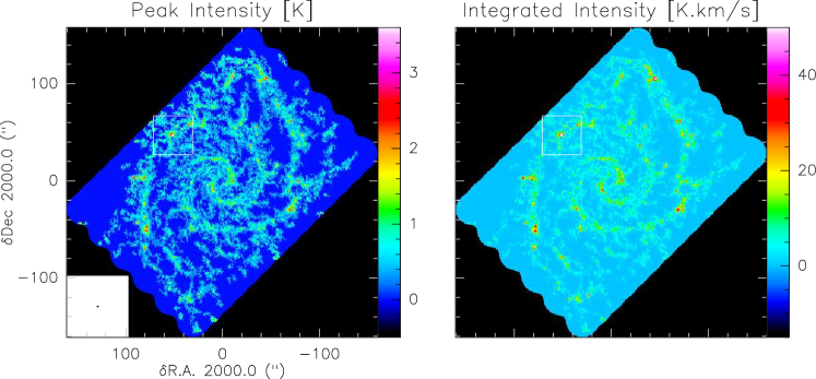
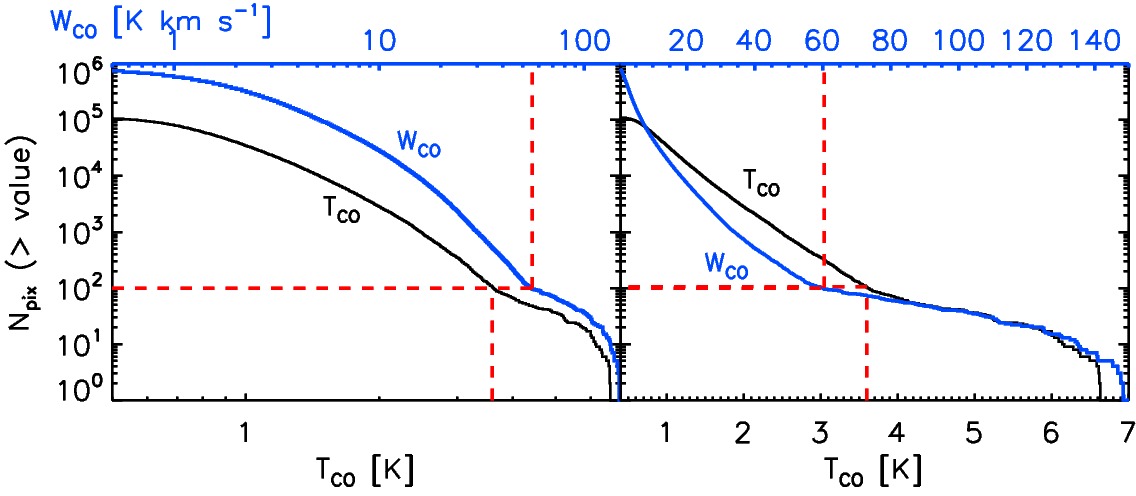
Figure 1: Top: Spatial distribution of the peak temperature (left) and integrated intensity (right) of the CO(2$-$1) line over the full observed field of view of NGC 628. The color scales a dynamic range of the peak temperature and integrated intensity, saturated to high intensity of 3.6 K and 45 K km s^-1. This is a compromise to show the spatial distribution of the $\sim 99.99\%$ of the pixels even though this may give the incorrect impression that other clouds in NGC 628 are as bright as the headlight cloud. The white square shows the position of the headlight cloud in NGC 628, which is zoomed in the left part of Fig. 2. Offset positions are from the galactic center, $\alpha:$ 01^h36^m41$\aas@@fstack{s}$72, $\delta:$ +15$\degr$46′59$\aas@@fstack{\prime\prime}$3 J2000. The beamsize is shown in the bottom left corner of the left panel. Bottom: Number of pixels whose CO(2$-$1) peak temperature $T_{\rm CO}$ (black curve) and integrated CO(2$-$1) intensity $W_{\rm CO}$ (blue curve) are above the value given in the bottom abscissa for $T_{\rm CO}$ and in the top abscissa for $W_{\rm CO}$, for the entire galaxy. The left panel shows the full range of values in logarithmic scale while the right one zooms in linear scale. The red dashed lines show the values corresponding to 100 pixels (or a surface of about $2^{\prime\prime}\times 2^{\prime\prime}$) in the CO map.

Additional observations were acquired in Cycle 2 to image the emission from the $J=1-0$ transition of ¹²CO (CO(1$-$0) hereafter), ¹³CO, C¹⁸O, HCO⁺, HCN, and HNC, as well as the CS(2$-$1) and HNCO 5(0,5)$-$4(0,4) lines. Three band 3 frequency setups at 90, 110 and 115 GHz were required to cover all these emission lines. The first setup at 90 GHz covers the $87.9-91.4$ GHz (LSB) and $99.6-103.2$ GHz (USB) frequency range. The second setup covers the $96-99.4$ GHz (LSB) and $108-111.7$ GHz (USB) range, and the third setup covers the $100.1-103.8$ GHz (LSB) and $112.3-115.5$ GHz (USB) range. The 110 GHz and 115 GHz setups target the CO lines that show both extended and compact emission. Thus, 7-m array and Total Power observations were performed in addition to the 12-m array observations in order to correctly recover the flux at all scales. Short-spacing observations for the 90 GHz set-up are available for NGC 628, but we chose not to incorporate them into the data cubes that we analyze here, because the 90 GHz setup targets lines mostly show compact emission structures.

The field-of-view covered by our observations at 90, 110, and 115 GHz was 232^′′$\times$170^′′, 240^′′$\times$150^′′, and 200^′′$\times$150^′′, respectively. Between 31 and 38 12-m antennas and between 9 and 10 7-m antennas were used during the different observations. The Total Power observations used simultaneously either 2 or 3 antennas. The same OFF as for the Cycle 1 was used during the On-The-Fly observations.

2.2.2 Reduction and Imaging

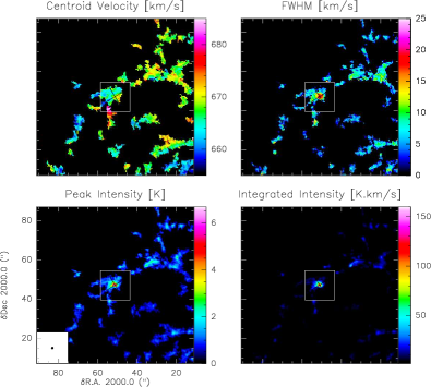
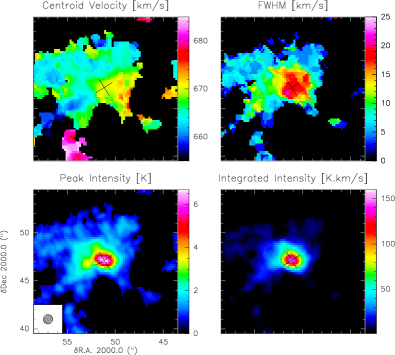
Figure 2: Spatial distributions of the moments of the CO(2$-$1) line centered over the headlight cloud. The 4 left panels show how this molecular cloud relates to the spiral arm, covering a field-of-view of 80″$\times$80″, while the 4 right panels zoom in on the molecular cloud itself. The beamsize is shown in the bottom left corner of the bottom left panels.

The data reduction recipes used for the 3 mm lines are much simpler than the ones used to reduce the CO(2$-$1). This is due to the fact that the 3 mm lines were reduced much before the recipes for the large program converged. In view of the satisfactory results obtained at relative low signal-to-noise ratio, we did not try to refine them. This section describes these simple recipes.

Data calibration for the Cycle 2 band 3 data was performed in CASA, versions 4.2.1 and 4.3.1 for the interferometric data, and 4.4 and 4.5 for the Total Power data. Interferometric calibration followed the recipes provided in the ALMA reduction scripts, as visual inspection showed that the scripts yielded a satisfactory calibration.

The CO and ¹³CO (1$-$0) data were then spectrally smoothed to 6 km s^-1. A signal mask was created from a CO(1$-$0) total power cube smoothed to an angular resolution of $60^{\prime\prime}$. The mask was created using the CPROPS signal detection algorithm, i.e. emission regions with a signal-to-noise ratio greater than 3 were identified and then extended to include contiguous pixels with a signal-to-noise ratio greater than 2. This mask was used to guide the deconvolution of the CO and ¹³CO (1$-$0) data.

A single-scale clean algorithm, as coded in the CASA task tclean, was applied to the 12 m+7 m data up to the point where the residual maximum fell below 1 mJy. The total power cube was used as an initial model. The resulting cleaned cube was then feathered with the total power cube.

The fainter lines were imaged at coarser spatial and spectral resolution (see Table 1 for details). Total power cubes were not used during the deconvolution (neither as models, nor for short-spacing correction) in these cases as the signal was barely or not at all detected in the single-dish observations.

2.3 Complementary MUSE data

We use MUSE observations to characterize the ionized gas and stellar content associated with the headlight cloud. MUSE is an optical IFU on the VLT in Paranal, Chile. Kreckel et al. (2016, 2018) present a detailed explanation of the strategy and data reduction of the MUSE observations of NGC 628. We summarize a few key aspects here.

The observations cover a wavelength range from 4800 to 9300 Å, which includes the H$\alpha$ and H$\beta$ emission lines and a large region of the optical stellar continuum. The velocity resolution is about 150 km s^-1. In the mode that we used, the field-of-view of the IFU is $1\arcmin\times 1\arcmin$ with $0\aas@@fstack{\prime\prime}2$ pixels. We paneled multiple fields-of-view to cover the whole inner part of the galaxy (see Kreckel et al., 2018). The seeing of the observations was $\sim 1$″($\sim 47$ pc in linear scale), with an astrometric accuracy of $0\aas@@fstack{\prime\prime}2$.

The H$\alpha$ emission line was obtained using the LZIFU pipeline (Ho et al., 2016), which simultaneously fits and subtracts the stellar continuum. All line fluxes quoted in this paper have been corrected for extinction. The emission line reddening has been inferred by comparing the observed H$\alpha$ to H$\beta$ line ratio to an intrinsic value of 2.86 (for case B recombination and an electron temperature of 10,000 K) under the assumption of a Fitzpatrick (1999) extinction curve with $R_{V}=3.1$. Typical values for E(B-V) are $\sim 0.5$ including for the headlight cloud.

3 Molecular gas in the headlight cloud

3.1 The CO(2$-$1) emission

Table 2: Physical properties of the ten most CO luminous clouds measured by CPROPS, sorted by decreasing luminous mass. Last line lists the parameters averaged in all molecular clouds in NGC 628. From the first to the eleventh column: cloud identification, cloud coordinates in R.A. and Dec., luminous CO mass, virial mass, radius, velocity linewidth, virial parameter, molecular gas mass surface density, CO(2$-$1)/CO(1$-$0) ratio, and measured distance to the closest corotation region. Column 12 lists the H$\alpha$ luminosity of the associated H ii region estimated from MUSE observations from Kreckel et al. (2017).

	Molecular gas										H ii region†
Cloud	R.A.	Dec.	Mlum	Mvir	Rad.	$\Delta_{v}$	$\alpha_{\rm vir}$	$\Sigma_{\rm mol}$	R21	Dcorot	LHα
ID	h:m:s	$\degr:\arcmin:\aas@@fstack{\prime\prime}$	105 $\mathrm{M_{\odot}}$	105 $\mathrm{M_{\odot}}$	pc	km s-1	–	$\mathrm{M_{\odot}}$ pc-2	–	kpc	erg s-1
L1⋆	01:36:45.328	15:47:48.48	204	91	184	16.3	0.5	192	0.70	0.00	6.3$\times$1039
L2	01:36:41.757	15:47:22.17	149	92	280	13.2	0.7	61	0.61	1.71	5.5$\times$1036
L3	01:36:47.144	15:46:08.77	142	73	193	14.2	0.6	121	0.71	0.37	7.1$\times$1038
L4	01:36:38.574	15:48:46.11	139	68	141	16.0	0.5	223	–††	0.00	8.2$\times$1038
L5	01:36:42.337	15:46:50.22	127	131	246	16.9	1.2	66	0.60	2.18	2.6$\times$1037
L6	01:36:42.974	15:47:23.85	118	83	302	12.1	0.8	41	0.60	1.35	8.6$\times$1036
L7	01:36:44.038	15:46:35.88	118	172	355	16.1	1.6	30	0.56	0.87	4.2$\times$1036
L8	01:36:36.942	15:46:31.21	105	63	145	15.2	0.7	159	0.61	0.00	6.6$\times$1037
L9	01:36:43.859	15:48:01.02	88	52	204	11.6	0.7	67	0.57	0.00	1.3$\times$1037
L10	01:36:41.309	15:46:59.40	86	89	212	15.0	1.2	61	0.63	2.50	7.7$\times$1036
NGC 628 Mean	–	–	14	22	91	10.3	2.1	56	0.54	–	–

^⋆Cloud 1 corresponds to the NGC 628 headlight.
^†Often there are multiple objects within a 150 pc region. We have listed the closest H ii region.
^†† Cloud L4 falls just outside the coverage of the CO(1$-$0) observations.

The top row of Fig. 1 presents ALMA maps of the CO(2$-$1) peak brightness and integrated intensity across NGC 628. The headlight cloud is located within an outer spiral arm, at an offset of $[47^{\prime\prime},51^{\prime\prime}]$ and a radial distance of 3.2 kpc from the galaxy center. The cloud is visible as the brightest peak in both panels of Fig. 1.

In the bottom row of Fig. 1, we plot pixel-wise cumulative distribution functions (CDFs) of the CO(2$-$1) peak brightness $T_{\rm CO}$ and the integrated intensity $W_{\rm CO}$ across the ALMA field-of-view. The CDF is a one-point statistic that quantifies how the emission in each map is distributed between low- and high-brightness regions (for detailed discussion of CO distribution functions we refer the reader to Hughes et al., 2013).

The headlight cloud stands out in both CDFs. For both $T_{\rm CO}$ and $W_{\rm CO}$, the distributions clearly show a change in slope for the 100 brightest pixels in the map, which we indicate with a red line. The sense is that above some high threshold, there is more bright CO emission than one would predict based on the rest of the galaxy. That is, the slope of the distribution function becomes flatter. All of these unusually bright pixels above either threshold belong to a region surrounding the headlight cloud.

This bright emission is notable for both its shape and location. We constructed equivalent CDFs for the peak brightness and integrated intensity maps of the CO(1$-$0) emission measured by the PAWS survey of M51 (Schinnerer et al., 2013; Pety et al., 2013) and the MAGMA survey of the Large Magellanic Cloud (LMC) (Wong et al., 2011), and of CO(2$-$1) emission measured by the IRAM 30-m survey of M33 (Druard et al., 2014), finding no similar features (see also Hughes et al., 2013, but note that this paper uses the probability distribution function rather than CDF formalism). In the mass distribution functions plotted by Sun et al. (2018, including NGC 628), bumps and features at high brightness are almost always associated with galaxy centers or dynamical environments like stellar bars. The headlight cloud lies in the outer part of a spiral arm, not associated with either the galaxy center or a stellar bar.

In Fig. 2, we zoom in on the headlight cloud. These maps show the CO(2$-$1) peak brightness, integrated intensity, centroid velocity and FWHM in a large region around the cloud (left) and in the immediate vicinity of the cloud (right). They show highly concentrated CO emission, with a compact, bright peak ($T_{\rm peak}>6\,$K over 1 square arcsecond $\sim 2,000$ pc²). This bright peak is surrounded by a more extended component with $T_{\rm peak}>1\,$K over $\sim 50$ square arcseconds or $\sim 100,000$ pc².

Morphologically, the cloud appears to be linked to other material in the spiral arm by four filaments. A fifth filament extends southwards from the cloud into the interarm region. The velocity field within the cloud, as traced by the centroid velocity, is relatively smooth, while the gas in the southern filament appears shifted to higher velocities compared to the cloud material.

The gas velocity dispersion in the cloud is high, and increases towards the cloud center: within $\sim 2$ arcseconds of the intensity peak, the FWHM linewidths are $>15\,\mbox{km\,s${}^{-1}$}$ with a maximum value of $24\,\mbox{km\,s${}^{-1}$}$. Typical CO(2$-$1) FWHM linewidths in the surrounding spiral arm are $\leq 10\,\mbox{km\,s${}^{-1}$}$ (see Fig. 2 top right panels).

3.2 GMC properties in NGC 628

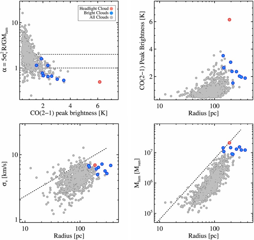
Figure 3: Scaling relations between physical properties of the molecular clouds in NGC 628: a) virial parameter as a function of CO peak brightness, b) CO peak brightness as a function of cloud size, c) linewidth as a function of size, and d) luminous mass as a function of size. In all panels, the headlight cloud is the red point, and the nine next most luminous ($M_{\rm lum}>8.6\leavevmode\nobreak\ \times\leavevmode\nobreak\ 10^{6}\,$$\mathrm{M_{\odot}}$) molecular clouds are blue. The horizontal dashed lines in the top left panels represent virial parameters of $\alpha=1$ and $\alpha=2$, values that are indicative of virialized and self-gravitating clouds respectively. The dashed line in the bottom left panel represents the size-linewidth relation reported by Solomon et al. (1987) for inner Milky Way clouds. The dashed line in the bottom right panel represents a mass surface density of $\Sigma_{\rm cld}=200\,$M_⊙ pc^-2.

Catalogs of giant molecular clouds (GMCs) for all the PHANGS-ALMA galaxies, including NGC 628, have been constructed and will be presented in a forthcoming paper (Rosolowsky et al., in prep). These catalogs are generated using the CPROPS algorithm (Rosolowsky & Leroy, 2006) to segment the CO(2$-$1) data cubes into individual molecular clouds and then measure the radius, linewidth, luminosity and other structural properties of each cloud.

3.2.1 The headlight cloud

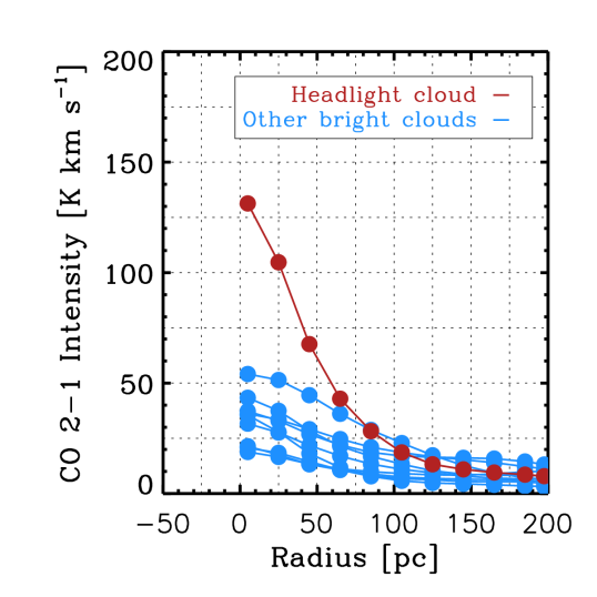
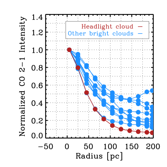
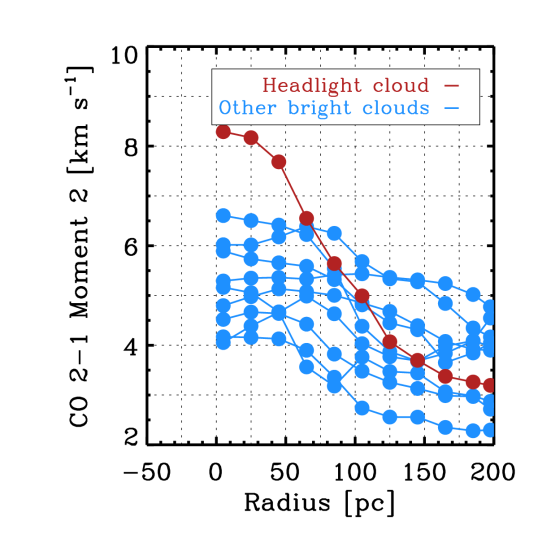
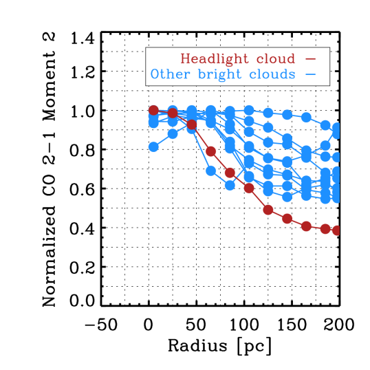
Figure 4: Profiles of mean integrated CO (2$-$1) intensity (top row) and mean CO (2$-$1) line width (bottom row) around the 10 most luminous clouds in NGC 628, with the headlight cloud highlighted in red. We use the second moment to characterize the line width, but note that other possible line width diagnostics (e.g. equivalent width) show similar trends to those plotted in the bottom row. For each cloud, we measure the azimuthally averaged quantity in radial bins centered on the cloud peak. The core of the headlight cloud is more than twice as bright as the next brightest massive cloud, and also has an enhanced central line width (left panels). In the right panels, we highlight the relative shape of the radial profiles by normalizing all measurements by the value at the cloud’s central position. The headlight cloud is more compact than the other massive clouds, though still moderately extended compared to the beam.

The cataloged radius and (FWHM) linewidth of the headlight cloud are 184 pc and 16.3 km s^-1 respectively. The measured radius of 184 pc has been deconvolved by the beam size, extrapolated to correct for sensitivity and blending effects, and then converted to the radius convention defined by Solomon et al. (1987), which implies multiplying the rms size by $1.91$ (for details see, Rosolowsky & Leroy, 2006). For a Gaussian shape, this implies a cloud FWHM size of $\sim 220$ pc.

The headlight cloud is the most luminous out of 850 clouds in the catalog, with a CO luminosity mass of $M_{\rm lum}=\alpha_{\rm CO}\,L_{\rm CO}=2.0\times 10^{7}$ $\mathrm{M_{\odot}}$. This mass assumes a CO(2$-$1)-to-H₂ conversion factor $\alpha_{\rm CO}=6.2$ $\mathrm{M_{\odot}}$ (K km s^-1 pc²)^-1, which is the Galactic CO(1$-$0) to H₂ conversion factor, 4.3 $\mathrm{M_{\odot}}$ (K km s^-1 pc²)^-1 (Bolatto et al., 2013), divided by 0.69, i.e., the CO(2$-$1)/CO(1$-$0) ratio measured in the headlight cloud (see Sect. 6.1). This CO(2$-$1)/CO(1$-$0) value is close to the nearby galaxy canonical value of 0.7 (e.g., Leroy et al., 2009, 2013; Saintonge et al., 2017) and to the mean ratio measured on kpc-scales in NGC 628 by the recent EMPIRE survey (Jiménez-Donaire et al., 2019, see also Table 5).

Treating the geometry as a three-dimensional Gaussian, the measured mass and radius of the headlight cloud imply an H₂ density of ${\rm n_{H_{2}}\sim 20}$ cm^-3. This is considerably lower than the critical density of CO(2$-$1) emission, even allowing for line trapping, and implies significant clumping or substructure within the cloud. The bulk physical parameters of the headlight cloud correspond to free-fall time and Mach number typical of massive giant molecular clouds. Using a mean density ${\rm n_{H_{2}}\sim 20}$ cm^-3, the free-fall time $t_{\rm ff}=\sqrt{3\pi/(32G\rho)}$ and crossing time $t_{\rm cross}=R/\Delta v$ are 8 and 11 Myr respectively. Assuming a gas temperature of $\sim$20 K (see Section 3.3.3), the measured linewidth corresponds to a Mach number of $\sim 42$.

3.2.2 Comparison with other luminous clouds in NGC 628

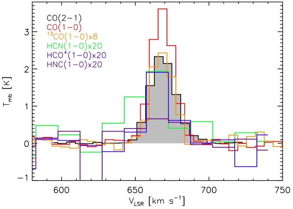
Figure 5: Left: Line profiles of all measured molecular gas tracers extracted at the position of the peak emission of each line, after convolving all data to the angular resolution of the ¹³CO(1$-$0). The CO(2$-$1) spectrum appears as the gray filled region. Other lines are scaled by the factors indicated in the legend to put them on the same plot. Right: RADEX output showing fits to the observed ratios among these lines. Blue, green, and red lines correspond to the observed HCN/¹³CO, HCN(1$-$0)/CO(2$-$1) and ¹²CO/¹³CO line ratios. The gray diamond marks the position on the RADEX [$n_{\rm H_{2}}$, $T_{\rm kin}$] grid where the $\chi^{2}$ is minimal, the best fit values. The dashed lines show the 95% confidence level of the $\chi^{2}$ fit that is smaller than the size of the diamond.

To place these values in context, Table 2 reports the physical properties (mass, radius, virial parameter) of the ten most luminous GMCs in NGC 628, as well as the mean value for NGC 628’s entire cataloged GMC population. We compare the headlight cloud to the full GMC population, highlighting these massive clouds, in Fig. 3.

The 184 pc radius of the headlight cloud is large but does not clearly distinguish the cloud from other massive clouds in NGC 628. The global linewidth of the headlight cloud (16.3 km s^-1) is also large but similar to that of the other high-mass GMCs in NGC 628. As a result, in the bottom left panel of Fig. 3, the headlight cloud clusters with the other massive clouds at the high end of the line width-size relation.

In contrast, the headlight cloud does stand out in surface density. The bottom right panel of Fig. 3 shows that the mass surface density of the headlight cloud, estimated from the luminous mass, is higher than any other massive cloud but one and among the highest in the galaxy. This value, $\Sigma_{\rm CO}\sim$ 190 ${\rm M}_{\odot}\,{\rm pc}^{-2}$, is roughly three times greater than the average value for all GMCs in NGC 628.

The most exceptional property of the CO(2$-$1) emission in the headlight cloud is its peak brightness, i.e., the intensity of the brightest pixel in the cloud at the $\sim 1\arcsec$ resolution of our PHANGS-ALMA CO(2$-$1) data. In the top row of Fig. 3, the headlight cloud (in red) clearly separates from the other massive clouds (in blue), with a peak brightness of almost $7$ K. This is roughly twice the peak brightness of the other massive clouds and the highest value found for any cloud in the galaxy.

A consequence of the headlight cloud’s high surface density and high brightness is that the cloud appears tightly bound. The virial parameter of the headlight cloud, estimated from the ratio between the cloud’s CO luminous mass and the virial mass $\alpha_{\rm vir}$=5$\sigma_{\rm v}^{2}$R/GM_lum is low, 0.5. This is low compared to both most other clouds in the galaxy and the value expected for virialized ($\alpha_{\rm vir}=1$) or marginally bound ($\alpha_{\rm vir}=2$) GMCs. We note that the low virial parameter of the headlight cloud (and many of the other massive clouds) appears to be part of a systematic trend in NGC 628 for the GMC virial parameters to decrease with increasing peak brightness (top left panel of Fig. 3) and $M_{\rm lum}$ (not shown). This trend needs to be interpreted with care: the scatter at low brightness is partly due to the impact of marginal resolution on these measurements, while CO brightness also enters in the denominator of the virial parameter via the definition of $M_{\rm lum}$. Nevertheless, simulations do predict mass- and environment-dependent variations in cloud virialization (e.g. Federrath & Klessen, 2012), and we plan to investigate these trends in more detail using the full PHANGS-ALMA sample in a future paper.

Figure 3 shows that the headlight cloud has a large size and velocity dispersion like the other massive clouds in NGC 628, but an exceptionally bright core. This implies a unique profile for the cloud within the NGC 628 GMC population. Figure 4 examines this profile in more detail. The top left panel plots the CO(2$-$1) integrated intensity as a function of distance away from the brightest pixel in the cloud for each of the 10 most massive GMCs in NGC 628. The top right panel shows the same, but normalizing all clouds by the integrated intensity at the cloud centre. The bottom row of Fig. 4 is similar, but here we plot radial profiles of the CO(2$-$1) line width instead of integrated intensity. We use the second moment to parameterize the cloud line width in Fig. 4, but a similar result is obtained using other line width diagnostics.

Figure 4 shows that the headlight cloud has the brightest core among all the massive clouds. The core is surrounded by an extended envelope of lower intensity emission – leading to the large size estimated by CPROPS – but the top right panel shows that in relative terms, the headlight cloud has the most compact profile of all massive clouds in NGC 628. The velocity profile of the headlight cloud is also distinctive, with an enhanced central line width and a steeper decrease in the line width between the cloud’s center and edge.

Figures 3 and 4 thus tend to reinforce the visual impression from Fig. 1 that the CO emission associated with the headlight cloud has exceptional properties. After integrating over the extent of the CPROPS-identified cloud, the headlight cloud resembles other massive clouds in NGC 628 in terms of size, line width, and mass. Yet looking more closely, it stands out due to its compact profile and enhanced central line width. Below, we show that the headlight cloud’s compact CO-bright core is coincident with a bright H ii region. This, combined with its apparently strong self gravity, indicates a massive star-forming region caught in the early stages of forming stars, and perhaps a potential birth site of massive clusters.

3.3 Other molecular emission lines

In addition to CO(2$-$1), we observed NGC 628 in CO(1$-$0), ¹³CO(1$-$0), CS(5$-$4), HCO⁺(1$-$0), HCN(1$-$0) and HNC(1$-$0). The ratios among these lines potentially allow us to further constrain the physical conditions (e.g., density, temperature) within the headlight cloud.

3.3.1 Observed line ratios in the headlight cloud

Table 3: Best-fit parameters of the molecular line profiles. The line profiles are extracted at the position of the peak of the headlight cloud after convolution to a common angular resolution. The quoted uncertainties in the parameters correspond to the errors in the Gaussian fits, and the FWHM is reported as $\Delta v$. At 9.6 Mpc, the $3\mbox{${}^{\prime\prime}$}5\times 2\mbox{${}^{\prime\prime}$}6$ Gaussian beam of the matched resolution input data corresponds to a physical area of $\sim 22,300$ pc².

	At peak, convolved to 13CO beam
Line	TPeak	VLSR	$\Delta$v
	[K]	[km s-1]	[km s-1]
CO(2$-$1)	2.52$\pm$0.02	668.3$\pm$0.1	19.5$\pm$0.2
CO(1$-$0)	3.64$\pm$0.11	668.3$\pm$0.3	18.1$\pm$0.6
13CO(1$-$0)	0.51$\pm$0.02	668.2$\pm$0.4	17.7$\pm$0.9
HCO+(1$-$0)	0.10$\pm$0.01	666.8$\pm$1.8	20.4$\pm$3.0
HCN(1$-$0)	0.09$\pm$0.02	660.4$\pm$2.7	32.2$\pm$6.5

Table 4: Line ratios at the peak of the headlight cloud. The line ratios are calculated using (i) the peak brightness and (ii) the integrated intensity of each emission line, as determined by a Gaussian fit to the line profile (see Table 3). The line profiles are extracted at the position of the peak of the headlight cloud after convolution to a common angular resolution.

Ratio	Peak	Integrated
$\dfrac{\rm CO(2-1)}{\rm CO(1-0)}$	0.70	0.75
$\dfrac{\rm{}^{12}CO(1-0)}{\rm{}^{13}CO(1-0)}$	7.2	7.3
$\dfrac{\rm HCO^{+}(1-0)}{\rm HCN(1-0)}$	1.1	0.7
$\dfrac{\rm HCO^{+}(1-0)}{\rm{}^{12}CO(1-0)}$	0.028	0.031
$\dfrac{\rm HCN(1-0)}{\rm{}^{12}CO(1-0)}$	0.025	0.043
$\dfrac{\rm HCN(1-0)}{\rm{}^{13}CO(1-0)}$	0.2	0.3

Table 5: ¹³CO/¹²CO(1$-$0), CO(2$-$1)/CO(1$-$0), HCO⁺/HCN and HCN/CO(1$-$0) line ratios for the different sources displayed in Figure 6. For nearby galaxies from the EMPIRE survey, the average ratios are given for entire galaxies, disks and centers. The physical sizes used to derive these ratios are also listed.

Source	12CO/13CO(1$-$0)				CO(2$-$1)/CO(1$-$0)				HCO+/HCN(1$-$0)				HCN/CO(1$-$0)				Ref.†
	Size	Mean ratio			Size	Mean ratio			Size	Mean ratio			Size	Mean ratio
Headlight	140 pc	7.20			140 pc	0.70			140 pc	1.0			140 pc	0.03			This work
Orion B	6.5 pc	6.50			6.5 pc	0.75			6.5 pc	1.10			6.5 pc	0.92			S94,P17
30 Dor-10	8 pc	6.47			10 pc	1.07			1.5 pc††	5			1.5 pc††	0.14			P12,J98,A14
EMPIRE galaxies		Gal.	Disk	Cen.		Gal.	Disk	Cen.		Gal.	Disk	Cen.		Gal.	Disk	Cen.	C18, JD
NGC 6946	0.9 kpc	13.8	13.5	15.2	1.1 kpc	0.65	0.64	0.68	1.1 kpc	1.06	1.19	0.87	1.1 kpc	0.73	0.50	1.14
NGC 5194	1.0 kpc	10.3	9.9	8.2	1.2 kpc	0.73	0.81	0.80	1.2 kpc	0.75	0.97	0.65	1.2 kpc	1.11	1.17	2.26
NGC 5055	1.0 kpc	9.3	8.5	7.2	1.3 kpc	0.59	0.59	0.68	1.3 kpc	0.33	0.35	0.90	1.3 kpc	1.19	1.07	0.71
NGC 2903	1.2 kpc	10.3	11.0	12.3	1.4 kpc	0.63	0.64	0.68	1.4 kpc	0.53	0.42	0.72	1.4 kpc	0.92	0.83	1.38
NGC 3627	1.2 kpc	12.0	12.2	15.2	1.5 kpc	0.48	0.47	0.48	1.5 kpc	0.90	0.87	0.91	1.5 kpc	0.76	0.59	0.70
NGC 0628	1.3 kpc	13.2	13.5	9.9	1.5 kpc	0.61	0.64	0.57	1.5 kpc	0.55	0.47	0.89	1.5 kpc	0.54	0.72	0.63
NGC 3184	1.5 kpc	10.2	10.7	11.2	1.9 kpc	0.53	0.53	0.52	1.9 kpc	0.52	0.55	0.77	1.9 kpc	0.42	0.39	0.62
NGC 4321	1.9 kpc	10.3	10.3	10.9	2.3 kpc	0.57	0.56	0.62	2.3 kpc	0.90	1.03	0.75	2.3 kpc	1.14	0.84	1.57
NGC 4254	1.9 kpc	11.0	10.5	8.4	2.3 kpc	0.74	0.74	0.75	2.3 kpc	1.19	1.23	0.79	2.3 kpc	0.75	0.70	1.23

^†S94: Sakamoto et al. (1994); P17: Pety et al. (2017); P12: Pineda et al. (2012); J98: Johansson et al. (1998); A14: Anderson et al. (2014); C18: Cormier et al. (2018); JD: Jiménez-Donaire et al. (2019).
^†† The lines were observed at an angular resolution corresponding to 29 pc.

The headlight cloud is detected in all molecular tracers except CS(5$-$4). Moreover, it is the only source detected in these tracers in the 12-m ALMA observations. The locations of the emission peaks for the different molecular lines match to within $<1$″ for the CO lines and to within $1\aas@@fstack{\prime\prime}8$ for the high density tracers. These higher density tracers also have low signal-to-noise ratios (see Fig. 13). As a result it remains unclear whether the offsets are significant. In the remainder of this article, we will consider that the peaks for all lines are spatially coincident within our current measurement accuracy. As a consequence, the left panel in Fig. 5 shows the line profiles extracted at the position of the peak emission of each molecular line. To make a fair comparison, we first smooth all images to match the resolution of the lowest resolution dataset, ¹³CO(1$-$0), before extracting the line profile at the emission peak (See Fig. 14).

We fit a single Gaussian profile to each line in Fig. 5 and report the results in Table 3. We do not include the values for HNC(1$-$0), since no reliable fit could be obtained. The centroid velocities and linewidths of all tracers are in good agreement, although HCN appears somewhat broader than the other lines. We have verified that this is not due to the hyper-fine structure of the HCN(1$-$0) line, but it may be an artifact of the limited velocity resolution and sensitivity of the HCN data. Table 4 lists the peak brightness and integrated intensity line ratios for different combinations of the emission lines. We use these ratios in Section 3.3.3 to derive an estimate of the density and temperature of the molecular gas in the headlight cloud.

3.3.2 Comparison to literature line ratios

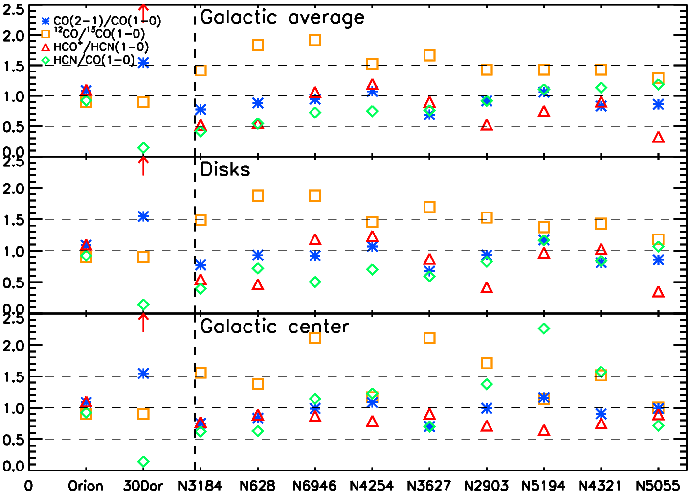
Figure 6: Line ratios observed in different sources, normalized to the values measured for the headlight cloud in NGC 628. Yellow, blue, red and green symbols correspond to the ¹²CO/¹³CO, CO(2$-$1)/CO(1$-$0)  HCO⁺/HCN and HCN/CO(1$-$0) line ratios. The values given for 30 Dor correspond to the values in the 30 Dor-10 molecular cloud. The red arrow for 30 Dor marks that the HCO⁺/HCN ratio is higher than 2.5. See Table 5 for the absolute values for these line ratios and their references.

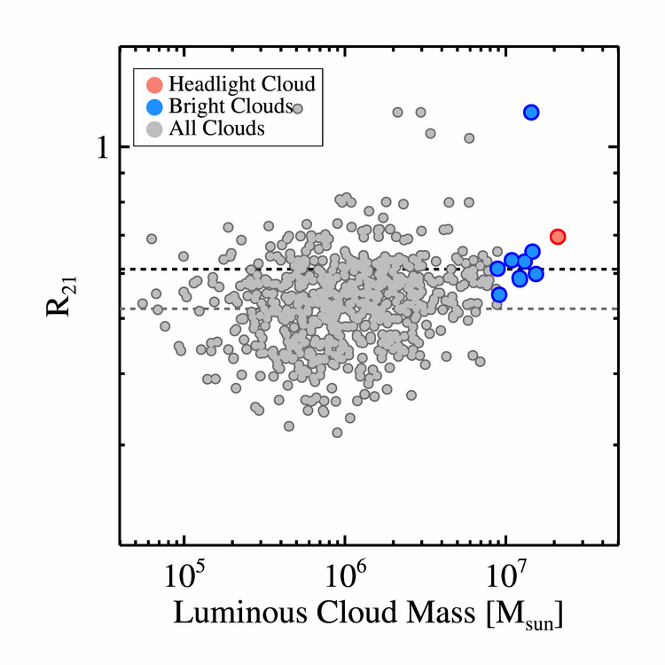
Figure 7: The CO(2$-$1)/CO(1$-$0) ratio measured on 140 pc scale at the positions of clouds in NGC 628. As in Figure 3, the headlight cloud is the red point, and the nine next most luminous ($M_{\rm lum}>8.6\leavevmode\nobreak\ \times\leavevmode\nobreak\ 10^{6}\,$$\mathrm{M_{\odot}}$) molecular clouds are blue. The kpc-scale estimate for CO(2$-$1)/CO(1$-$0) in NGC 628 measured by EMPIRE is indicated with a dashed black line, and the average value for the cloud-scale measurements is represented by a dashed gray line. The CO(2$-$1)/CO(1$-$0) measurements in this plot use the peak brightness of the CO(1$-$0) and CO(2$-$1) lines within a $3\aas@@fstack{\prime\prime}2\times 3\aas@@fstack{\prime\prime}2$ box centered on the cloud position.

Here we compare the line ratios that we measure for the headlight cloud to a compilation of line ratios in other Galactic and extragalactic sources. We compare to nine nearby spiral galaxies that are part of the EMPIRE survey (Bigiel et al., 2016), using the values determined by Cormier et al. (2018) and Jiménez-Donaire et al. (2019). We also compare to line ratios measured in Orion-B in the Milky Way (Sakamoto et al., 1994; Pety et al., 2017) and 30 Doradus in the LMC (Johansson et al., 1998; Pineda et al., 2012; Anderson et al., 2014). Table 5 lists these ratios, the associated spatial scales, and the references for the measurements.

Figure 6 shows the HCN/CO(1$-$0) line ratio in red, HCO⁺/HCN in green, ¹³CO/¹²CO in yellow and CO(2$-$1)/CO(1$-$0) in blue. In each case, we plot the line ratio in the comparison source normalized to the value estimated for the headlight cloud, so that it indicates a line ratio identical to the headlight cloud. From the top to bottom panel, we plot the data for entire galaxies, and for disk and center regions separately. We do not show data for the inter-arm or diffuse extended regions. This is why the galactic “average” values can sometimes be lower than both the disk and center values. The line ratios used in this plot and quoted in Table 5 are derived using different methods and on datasets with a range of resolution and sensitivities, and the values should therefore be interpreted with some caution. As described in Section 3.3, the values for headlight cloud are determined using the peak brightness of a Gaussian fit to line profiles extracted at a spatial scale of $\sim 140$ pc, whereas the values for the EMPIRE galaxies are ratios calculated using the integrated intensity of an average line profile from within a kpc-scale aperture. A comparison between ratios measured at similar scales will only be possible when more high angular resolution data in nearby galaxies will become available. Using current data, the first striking point is that the ratios mostly exhibit the same order of magnitude independent of scale. This probably suggests that the emission of the different lines is co-spatial to first order, i.e., the lines arise from the same molecular gas phase. They are thus affected by beam dilution in similar ways. Detailed analysis of second order variations of the ratios may indicate other physical and chemical processes.

In extragalactic work, the ratio between HCN/CO ratio is often used as an indicator of gas density. The ratio measured on 140 pc scale in the headlight cloud, HCN/CO = $0.025$ to 0.04 is in broad agreement with values found in galaxy disks (e.g., Usero et al., 2015; Gallagher et al., 2018). It is higher than the value measured on larger scales from the EMPIRE full-disk map of NGC 628 (Jiménez-Donaire et al., 2019), for which the mean HCN/CO ratio is $\sim 0.015$. This can be seen from low normalized value, $\sim 0.5$, of the green symbol in NGC 628 in Fig. 6, showing that the HCN/CO in the headlight cloud is about two times higher than the galaxy-averaged value. Assuming that the HCN/CO ratio highlights dense gas, the headlight cloud appears to be denser than its surroundings, with more dense, HCN-emitting gas, consistent with the compact structure at the core of the cloud structure measured in CO.

The HCO⁺/HCN ratio is more variable among the EMPIRE survey targets. The HCO⁺/HCN ratio in the headlight cloud is about twice the disk-averaged value within NGC 628 (0.55), and closer to the value estimated towards NGC 628’s central region (0.89). The HCO⁺/HCN ratio in the headlight cloud is similar to the average ratio observed in Orion B (1.1), but significantly less than the ratio observed in the 30 Dor-10 molecular cloud (5). We note that HCO⁺/HCN ratios ranging between 3 and 10 have been reported for several star-forming regions in the LMC (including e.g. N159W, N44, N105, and other clouds near 30 Dor, Seale et al., 2012; Anderson et al., 2014) and the low metallicity Local Group dwarf IC 10 (Nishimura et al., 2016; Braine et al., 2017; Kepley et al., 2018). This may indicate a metallicity dependence of this ratio, since HCO⁺/HCN values close to unity are observed in massive star-forming regions in our Galaxy (e.g. W51 Watanabe et al., 2017), and values between 0.5$-$2 on larger scales in starburst galaxies (e.g., Imanishi et al., 2007; Krips et al., 2010; Bemis & Wilson, 2019).

The ¹²CO/¹³CO line ratio in the headlight cloud is $7.2$, which is comparable to the value in Orion B (Pety et al., 2017) and in the 30 Dor-10 molecular cloud. The EMPIRE measurements for NGC 628 and other nearby spiral galaxies are systematically higher, which we attribute to the lower filling factor of ¹³CO emission within the EMPIRE resolution element ($27^{\prime\prime}\sim 1$ to 2 kpc).

The CO(2$-$1)/CO(1$-$0) ratio in the headlight cloud is $\sim 0.7$, which is close to the standard value for resolved observations in the Milky Way (including the Orion B cloud, see e.g., Sakamoto et al., 1994, 1997; Yoda et al., 2010), and in nearby galaxies (e.g., Eckart et al., 1990; Leroy et al., 2009, 2013; Cormier et al., 2018). The 30 Dor 10 molecular cloud in the LMC (Pineda et al., 2012) stands out as having a CO(2$-$1)/CO(1$-$0) ratio close to unity, while the mean ratio for the kpc-scale EMPIRE measurements in NGC 628 and other nearby spiral galaxies is slightly lower, $\sim 0.6$, than in the headlight cloud. The EMPIRE CO(2$-$1)/CO(1$-$0) measurements show some variation between and within galaxies: in NGC 5055 and NGC 4321, the CO(2$-$1)/CO(1$-$0) ratio increases towards the galaxy centers, but the opposite trend is seen for NGC 628.

Since the kpc-scale of the EMPIRE measurements can obscure cloud-scale variations of CO(2$-$1)/CO(1$-$0) within NGC 628, we measured the mean CO(2$-$1)/CO(1$-$0) ratio within a $3\aas@@fstack{\prime\prime}2\times 3\aas@@fstack{\prime\prime}2$ box, centred on the positions of the GMCs identified in NGC 628 (see Section 3.2). To be consistent with the measurements of the headlight cloud in Section 3.3.1, the line ratios were defined using the peak brightness of CO(1$-$0) and CO(2$-$1) data cubes that had been smoothed to common (round beam) resolution of $3\aas@@fstack{\prime\prime}2$. We restricted our measurement to pixels where the signal-to-noise at the line peak was greater than 5 in both tracers, and we rejected clouds where our analysis box contained less than 10 valid pixels. We list the cloud-scale CO(2$-$1)/CO(1$-$0) measurements for NGC 628’s ten most luminous clouds in Table 2, and we plot all the cloud-scale measurements of CO(2$-$1)/CO(1$-$0) versus the cloud luminous mass in Fig. 7. From this analysis, it is clear that kpc-scale averages hide genuine local variations in CO(2$-$1)/CO(1$-$0): we find a mean cloud-scale value of CO(2$-$1)/CO(1$-$0) in NGC 628 of 0.54, with a standard deviation of $0.10$ in the cloud-scale measurements. We note here that the headlight cloud has a relatively high CO(2$-$1)/CO(1$-$0) value relative to the rest of NGC 628’s cloud population, but defer a detailed investigation of the physical origin of CO(2$-$1)/CO(1$-$0) variations on sub-kpc scales to a future paper (Saito et al., in prep).

3.3.3 LVG modelling

Here we estimate the typical density and kinetic temperature of the molecular gas of the headlight cloud using a Large Velocity Gradient (LVG) analysis of some of the line ratios measured at the cloud’s emission peak (see Table 4). We use RADEX, a public LVG radiative transfer code. We assume an expanding sphere geometry, a velocity linewidth of 20 km s^-1 (this is the mean value of the observed linewidth for all tracers, see column 4 of Table 3), and a background temperature of 2.73 K. The H₂ column density is set to $N_{\rm H_{2}}$ to 9$\times 10^{21}$ cm^-2, which is the value obtained assuming a CO luminous mass of 2$\times 10^{7}$ $\mathrm{M_{\odot}}$ and radius of 180 pc (see Sect. 3.2.1). We first compute a grid of LVG models, which covers a kinetic gas temperature range of $T_{\rm kin}=10-160$ K, and molecular gas density range of $n_{\rm H_{2}}$=10² $-$ 10⁷ cm^-3. We fit the ¹²CO(1$-$0)/¹³CO(1$-$0) ratio as a good tracer of temperature variations, HCN(1$-$0)/¹³CO(1$-$0) as a tracer of gas density variations and HCN(1$-$0)/¹²CO(2$-$1) as a confirmation of the implied temperature to density ratio. The molecular abundances are fixed to their typical Galactic values, i.e., [¹²CO]/[H₂] = 3$\times 10^{-4}$, [¹²CO]/[¹³CO] = 70, and [HCN]/[H${}_{2}]=5\times 10^{-9}$ (Blake et al., 1987; van Dishoeck & Black, 1988).

We do not attempt to fit the CO(2$-$1)/CO(1$-$0), and HCO⁺(1$-$0)/HCN(1$-$0) ratios as they are difficult to interpret. Indeed, while the ¹²CO lines are optically thick, the energy difference between the J=2$-$1 and 1$-$0 levels is only 17 K. The latter property makes the CO(2$-$1)/CO(1$-$0) ratio mostly sensitive to cold gas, while the former property favors tracing diffuse gas at typical temperature of 80 K. The HCO⁺/HCN ratio is also difficult to interpret because it is sensitive to the relative abundance of these species, which vary with environment by an order of magnitude (Goicoechea et al., 2018).

The right panel of Fig. 5 shows the result of the fit of the different line ratios as a set of color-coded thick lines for the possible solutions and thin lines showing the 95% confidence interval. These curves intersect at $n_{\rm H_{2}}\sim 5\times 10^{4}$ cm^-3 and $T_{\rm kin}\sim 20$ K. This is more than three orders of magnitude greater than the average H₂ density estimated from the cloud mass and diameter quoted above. Assuming that 10 to 100% of the headlight cloud’s mass has this typical density and that the geometry is spherical, this yields a typical radius ranging from 15 to 34 pc. This gas has a typical thermal pressure of $10^{6}$ K cm^-3.

While this solution provides a good fit to the different line ratios, the RADEX-predicted CO(2$-$1) brightness is about three times larger than what is measured. We note this as a caveat to the inferred physical conditions, and consider our results for the cloud density and pressure as order-of-magnitude estimates. In view of the uncertainties in the beam filling factor of the different emission lines, the appropriate $X_{\mathrm{CO}}$ value, the molecule abundances, and the density distribution adopted in the LVG model, it is difficult to justify more sophisticated modelling with the current set of molecular line data.

4 Current stellar feedback

In this section, we characterize the H ii region associated with the headlight cloud. In particular, we estimate the typical age and mass of the associated young stellar population and we compute order-of-magnitude pressures related to stellar feedback. More detailed modelling is beyond the scope of this paper. It will be the subject of another forthcoming one.

4.1 The headlight cloud’s H ii region

The headlight cloud spatially coincides with the most luminous H ii region within the footprint of our MUSE observations. H$\alpha$ emission from this region closely resembles the CO emission in both morphology and kinematics, suggesting that the H ii region is still embedded within the cloud. To within an accuracy of 1″ (i.e., 47 pc), the two distributions peak at the same position. Figure 8 shows that the velocity structure of the molecular and ionized gas is also very similar.

As in CO, the H$\alpha$ emission associated with the headlight cloud is the brightest region in the galaxy. This region also appears bright relative to any simple extrapolation of the distribution of intensities from fainter regions. We show this in Fig. 9. There, we plot pixel-wise CDFs of the H$\alpha$ intensity $I_{\rm H\alpha}$ and $W_{\rm CO}$ for the entire galaxy.

Figure 9 shows that, like the CO emission, the H$\alpha$ emission has a bump at high intensities. The sense of this bump is that there are more bright pixels than one would expect base on extrapolating from lower intensities. The bump is specifically associated with the 45 brightest pixels in the H$\alpha$ map, which we mark with a green line in Fig. 9. These pixels are all associated with the headlight cloud. They belong to a region 2.3 square arcseconds in area that spatially correlates with the brightest CO peak.

4.2 Young stellar content

Figure 8: Maps of the velocity centroid of the H$\alpha$ and CO(2$-$1) emission for the region surrounding the headlight cloud. The maps are constructed after subtracting a model for the galaxy’s rotation (Lang et al., in prep). The contours correspond to the H$\alpha$ and CO integrated emission: black (white) contours in the left (right) panel are the CO(2$-$1) contours, white contours in the left panel are H$\alpha$ contours. The H$\alpha$ seeing and the restored CO(2$-$1) beam are indicated in the bottom-left part of each panel.

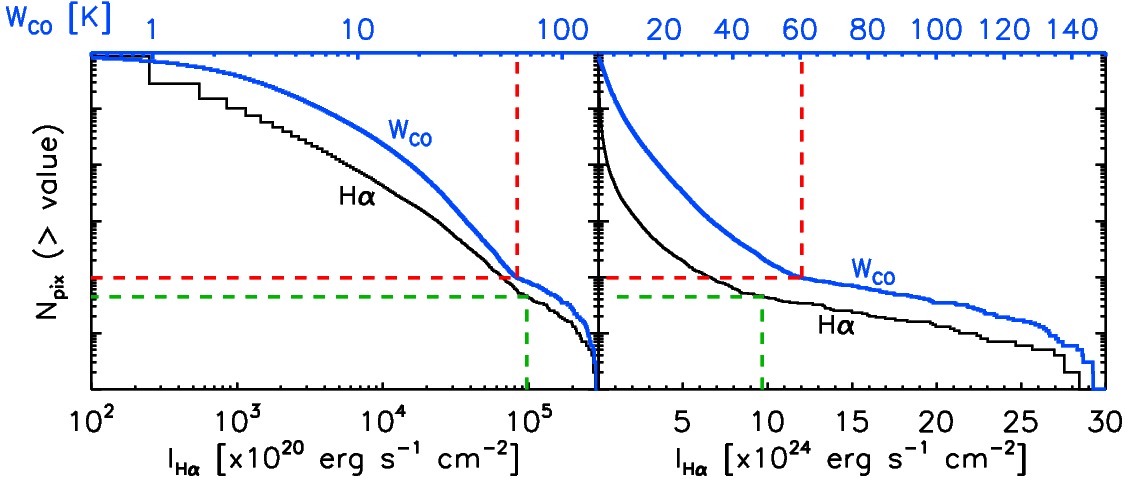
Figure 9: Number of pixels whose integrated H$\alpha$ intensity $I_{\rm H_{\alpha}}$ (black curve) and integrated CO(2$-$1) intensity $W_{\rm CO}$ (blue curve) are above the value given in the bottom abscissa for $I_{\rm H\alpha}$ and in the top abscissa for $W_{\rm CO}$, for the entire galaxy. The left panel shows the full range of values in logarithmic scale while the right one zooms in linear scale. The red dashed lines are as in Fig. 1. The green dashed lines show the values corresponding to 45 pixels (or a surface of about $1\aas@@fstack{\prime\prime}5\times 1\aas@@fstack{\prime\prime}$5) in the H$\alpha$ map.

The extinction-corrected H$\alpha$ luminosity associated with the headlight cloud (Kreckel et al., 2016, 2018) implies a SFR of 0.034 $\mathrm{M_{\odot}}$ yr^-1 assuming a constant star formation history. This is likely a lower limit since the bulk of the star formation activity may still be embedded. Moreover, the star formation history in the headlight cloud region may be better described as an instantaneous burst (see below).

We use the above SFR estimate to assess the local molecular gas depletion time $\tau_{\rm dep}^{\rm mol}\equiv M_{\rm mol}/{\rm SFR}$, finding $\tau_{\rm dep}^{\rm mol}\sim 0.6\,$Gyr using $2.0\times 10^{7}$ M_⊙ mass of the cloud. For comparison, we estimate $\tau_{\rm dep}^{\rm mol}\sim 1.6$ Gyr for the $1$ kpc region around the headlight cloud and $\sim 1.5$ Gyr for the whole area mapped by ALMA (both consistent with previous work by Leroy et al., 2008; Bigiel et al., 2008; Leroy et al., 2013; Kreckel et al., 2018). The latter values represent a large-scale equilibrium rate, while the former shorter value probably represents a small spatial-scale snapshot that reflects the current evolutionary state of the headlight (see Schruba et al., 2010; Kruijssen & Longmore, 2014; Kruijssen et al., 2018).

Table 6: Estimated physical properties of the H ii region and young stellar population embedded in the headlight cloud in NGC 628.

Name	Symbol	Value
H$\alpha$ luminosity	LHα	$6.3\times 10^{39}$ erg s-1
H$\alpha$ region radius	—	142 pc
H$\alpha$ line width	$\Delta$v	$\sim$50 km s-1
H$\alpha$ equivalent width	WHα	517 Å
Ionizing photon production rate	Nion	$4.6\times 10^{51}$ phot. s-1
Young star mass	Mcl	$3\times 10^{5}$ $\mathrm{M_{\odot}}$
Young star bolometric luminosity	Lcl	$4\times 10^{8}$ L⊙
Young star typical age	—	$2-4$ Myr

We can obtain a sharper picture of the recent star formation embedded within the headlight cloud by comparing observed properties to Starburst99 (S99) models assuming an instantaneous burst (Leitherer et al., 1999). In this case, our best constraint on the age comes from the equivalent width of the H$\alpha$ line, and our best constraint on the mass comes from the number of ionizing photons produced, as indicated by the total H$\alpha$ emission. The observations were compared to models using a solar metallicity, an instantaneous burst of star formation of 10⁶ $\mathrm{M_{\odot}}$, and a Kroupa initial mass function (IMF).

The age is estimated to be 4 Myr from the measured H$\alpha$ equivalent width (EW) of $517$ Å. This is an upper limit since S99 does not yield accurate age measurements when the region is younger than $4$ Myr. The MUSE spectrum of this H ii region shows the presence of the C IV line at $\lambda$5801-12Å. This line is a specific feature of Wolf-Rayet stars, which are present in stellar populations aged between 2 and 6 Myr. Combining both results, the age of the young stellar population is constrained to 2${-}$4 Myr.

The mass in young stars is estimated from the number of ionizing photons, $N_{\rm ion}$ they produce, itself estimated from the integrated extinction-corrected H$\alpha$ luminosity of the headlight cloud’s H ii region $L($H$\alpha)=6.3\times 10^{39}$ erg s^-1. Using Eq. 5 from Calzetti et al. (2010), this luminosity yields $N_{\rm ion}=4.6\times 10^{51}\,$photon s^-1. The S99 single stellar population models assuming this value of $N_{\rm ion}$ yield a stellar mass as large as $\sim 3\times 10^{5}$ $\mathrm{M_{\odot}}$ and a bolometric luminosity of $L_{\rm cl}=4\times 10^{8}$ L${}_{\odot}.$ The measured and estimated properties of the young massive stellar population embedded in the headlight cloud are summarized in Table 6.

4.3 Stellar Feedback

The spatial coincidence of a massive young stellar population and massive GMC indicates that these stars have not yet dispersed their parent molecular cloud. In this section, we investigate the potential feedback mechanisms that may lead to the disruption of the headlight cloud, adopting the properties for the cloud and the young stellar population listed in Tables 2 and 6, respectively.

The population of Wolf-Rayet stars will produce strong winds that will push away the low density ionized gas of the H ii region. In the simple spherically symmetric picture, this will results in a thin or thick shell of ionized gas surrounding an almost empty central region. The density in the shell will be higher than the mean density of the sphere, so that the ram pressure approximately balances the thermal pressure.

To examine the balance of forces in more detail, we start by assuming that the hot gas associated with the wind has been lost from the young stars, either because it has already radiatively cooled or because it has escaped through low density gaps in the shell (see e.g. Rogers & Pittard, 2013). This assumption is consistent with the fact that we do not find any signature of compact X-ray emission associated with the headlight cloud in Chandra and XMM-Newton observations (Liu, 2005; Owen & Warwick, 2009). It is also consistent with detailed models of the effects of stellar winds on molecular clouds, which typically find that the hot gas is lost within only $\sim 1$ Myr from the onset of the wind (see e.g. Rahner et al., 2017). The mechanical luminosity of the wind predicted by the S99 models is $L_{\rm mech}=4.9\times 10^{6}$ L_⊙. This can also be written in terms of the total stellar mass loss rate ($\dot{M}$) through

$$L_{\mathrm{mech}}=\frac{1}{2}v_{\mathrm{wind}}^{2}\dot{M},$$ (1)

where $v_{\rm wind}$ is the characteristic wind velocity. In the present case, the wind luminosity is dominated by the Wolf Rayet stars and so the wind velocity will typically be very large, i.e., $v_{\rm wind}\sim 2\times 10^{3}\,$km s^-1. This yields a mass loss rate $\dot{M}\sim 9.4\times 10^{23}\,$g s^-1. The ram pressure at radius $R$ is

$$P_{\rm ram,wind}=\frac{v_{\rm wind}\dot{M}}{4\pi R^{2}}.$$ (2)

Assuming that $R$ is the radius of the H ii region, we find $P_{\rm ram,wind}\sim 5.7\times 10^{5}\,$K cm^-3. This value depends on our assumed wind velocity, since $P_{\rm ram,wind}\propto v_{\rm wind}^{-1}$, but does not change by more than a factor of two for wind velocities in the range consistent with Wolf Rayet stars.

If some of the massive young stars have already exploded as supernovae (SN), these will also contribute to the total ram pressure. The importance of this contribution depends on the age of the young stellar population and the assumed star formation history. For our assumption of an instantaneous burst, the first supernovae occur at a time $t\sim 3.6$ Myr (Leitherer et al., 1999). The headlight cloud appears as a compact source in the non-thermal emission map at 3.1 GHz in Mulcahy et al. (2017), thus likely tracing synchrotron emission from supernovae. We can estimate the contribution that the associated supernovae make to the ram pressure from

$$P_{\rm ram,SN}=\frac{v_{\rm SN}\dot{M}_{\rm SN}}{4\pi R^{2}}.$$ (3)

Here $\dot{M}_{\rm SN}$ is the supernova mass loss rate, which we take from the S99 model, and $v_{\rm SN}$ is the terminal velocity of the supernova ejecta, which we take to be $10^{4}$ km s^-1, following Rahner et al. (2017). Note that this estimate is conservative, in that it neglects any contribution made by the pressure of the hot gas associated with the supernovae, consistent with our treatment of the stellar winds. For a young stellar population age of 4 Myr, this yields a ram pressure contribution $P_{\rm ram,SN}\sim 3.0\times 10^{5}\,{\rm K\,cm^{-3}}$, i.e., roughly half of the contribution coming from stellar winds. We recover similar results for other assumed ages in the range $3.6<t<6.0$ Myr.

At the radius of the H ii region, the wind ram pressure balances the thermal pressure due to the ionized photons (Pellegrini et al., 2007), provided that other sources of support (e.g. magnetic fields) are unimportant. If we assume that thermal pressure is the main source of support for the ionized shell, and that the gas has a typical H ii region temperature of $10^{4}\,$K, then it follows that the ionized gas must have a typical electron density of $n_{\mathrm{e}}\sim 30\,$cm^-3. If we assume that this density is achieved in a shell with radius $R_{H\textsc{ii}}$, we can also solve for the shell thickness $(dR)$ required to have ionization balance

$$N_{\mathrm{ion}}=\frac{4\pi}{3}\alpha_{B}n_{\mathrm{e}}R_{H\textsc{ii}}^{2}dR,$$ (4)

where $\alpha_{B}$ is the case B recombination coefficient. This gives $dR\sim 7\,$pc. Note that this is technically the thickness of the ionized portion of the shell: if the expansion of the shell has also swept up a substantial amount of neutral/molecular gas, then the full shell will be even thicker. Finally, we can calculate the mass of the ionized gas: $M_{\mathrm{ion}}\sim 6\times 10^{5}\,\mathrm{M_{\odot}}.$ The ionized gas thus does not contribute much to the overall mass budget. For comparison, Galván-Madrid et al. (2013) find that in W49 (one of the most massive GMCs in the Milky Way, albeit a factor 10 less massive than the headlight cloud) only $\sim 1\%$ of the total gas mass is in the ionized component, comparable to the value of a few percent we infer here for the headlight cloud.

The radiation pressure is estimated following Eq. 1 in Herrera & Boulanger (2017). For a radius defined by the H$\alpha$ emission, and assuming no trapping of the IR photons within the shell, the radiation pressure is $P_{\rm r0ad}=1.5\times 10^{5}$ K cm^-3. The turbulent pressure in the molecular gas, $P_{\rm turb}=\rho\sigma_{v}^{2}$, is estimated to be $P_{\rm turb}=1.9\times 10^{5}\leavevmode\nobreak\ {\rm K\leavevmode\nobreak\ cm^{-3}}$.

The magnetic pressure cannot be accurately computed, as we have no measurement of the magnetic field strength on the scale of the headlight cloud. If we adopt a value of $10\leavevmode\nobreak\ \mu$G, based on the kpc-scale measurements of Mulcahy et al. (2017), the resulting magnetic pressure is $P_{\rm mag}=2.9\times 10^{4}\,{\rm K\,cm^{-3}}$, implying that the field would not play a significant role in regulating the expansion of the H ii region (van Marle et al., 2015). It is possible that the cloud-scale magnetic field strength is larger than this, implying a larger magnetic pressure, but we do not expect $P_{\rm mag}$ to exceed the turbulent pressure unless the turbulence in the cloud is substantially sub-Alfvénic. Since it would be difficult to explain the large amounts of recent star formation if the cloud were strongly magnetically-dominated, we conclude that $P_{\rm mag}$ is unlikely to greatly exceed $P_{\rm turb}$.

The gravitational pressure exerted by the young stellar body and the molecular cloud itself is $P_{\rm grav}=3.6\times 10^{5}$ K cm^-3, following Eq. 5 in Herrera & Boulanger (2017), assuming a size defined by the CO emission. In this computation, we neglected the contribution of the ionized component as discussed above. Hence, the combined outward pressures, $P_{\rm turb}$, $P_{\rm ram}$ (winds and supernovae), and $P_{\rm rad}$, overcome the gravitational and magnetic pressures by a factor 2-4.

4.4 Comparison with 30 Dor in the LMC

We note that the properties of the H ii region in the headlight cloud are similar to N157A (Henize, 1956), the H ii region associated with the 30 Dor star-forming region, which is the largest and most active star-forming region in the Local Group. N157A has an ionizing photon rate of $N_{\rm ion}=4.5\times 10^{51}$ photon s^-1 and a size of $\sim$200 pc (Walborn, 1991); the H ii region in the headlight cloud has $N_{\rm ion}=4.6\times 10^{51}$ photon s^-1 and a radius of $\sim$140 pc (see Table 6). The age and mass of the embedded young stars in the headlight cloud are likewise comparable to 30 Dor’s central star cluster (R136), which is $\sim$1-3 Myr old and has a stellar mass of $4.5\times 10^{5}\,\mathrm{M_{\odot}}$ (Bosch et al., 2009). The molecular gas properties of these regions are quite different, however. The integrated ¹²CO(1$-$0) luminosity that is observed to be spatially projected onto N157A is $\sim 2.5\times 10^{5}$ K km s^-1 pc², corresponding to only $\sim 10^{6}\,\mathrm{M_{\odot}}$ of molecular gas for a Galactic CO-to-H₂ conversion factor (Wong et al., 2011; Johansson et al., 1998). The young stars in 30 Dor thus appear to have cleared out most of the molecular gas associated with the H ii region, contrary to the headlight cloud, for which we estimate a molecular mass of $\geq 10^{7}\,\mathrm{M_{\odot}}$.

5 The Galactic Environment of the Headlight Cloud

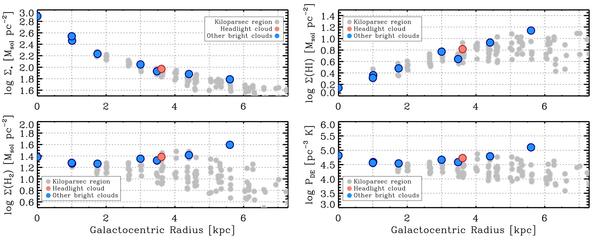
Figure 10: The headlight cloud in galactic context. Average surface density of stellar mass, atomic gas, molecular gas, and estimated dynamical equilibrium pressure in kiloparsec-sized apertures that cover the galaxy (from J. Sun et al. in preparation). Gray points show all apertures. Colored points show apertures that host one of the ten brightest clouds in the galaxy (red: the headlight cloud, blue: another bright cloud). The vertical spread of points at a fixed radius indicates azimuthal variations. The headlight cloud lies $\sim 3.5$ kpc from the galaxy center in an environment with unremarkable stellar mass or atomic gas content (see top row). However, this region does have among the highest molecular gas surface densities (bottom left) and dynamical equilibrium pressures (bottom right) anywhere in the galaxy. The headlight cloud and other bright cloud at similar radii are all associated with strong spiral features and so appear as the highest points at their radius. The fact that these clouds appear at large radius and comparatively low stellar surface density suggests that spiral structure and galactic dynamics (as opposed to only mean ISM pressure in a smooth disk) play a central role in setting the properties of these clouds.

Both the properties and location of the headlight cloud make it remarkable, as massive star-forming regions usually tend to appear at bar ends or galaxy centers. In this section, we examine the environment of the headlight cloud. First, we compare the properties of the region around the cloud to the rest of the galaxy. Then we consider how the cloud’s location relates to the dynamical structure of the galaxy.

5.1 Trends with Galactocentric Radius

In Fig. 10, we show the kpc-scale structure of NGC 628, highlighting the location of the headlight cloud. We plot the gas and stellar structure in NGC 628 as a function of galactocentric radius. Each point in Fig. 10 shows mean properties of NGC 628 estimated within a 1 kpc aperture (see Leroy et al., 2016; Sun et al., 2018; Utomo et al., 2018, for details). The apertures cover the galaxy. The measurements are taken from Sun et al. (in prep.).

The measurements shown in Fig. 10 are derived from multi-wavelength archival data for NGC 628. In addition to the PHANGS-ALMA CO (2$-$1) maps, we use THINGS HI 21 cm moment-0 map (Walter et al., 2008) to trace atomic gas distribution, S⁴G dust-subtracted $3.6\,\mu m$ image (Sheth et al., 2010; Querejeta et al., 2015) to trace stellar mass distribution, and GALEX-NUV and WISE band 3 images (presented in Leroy et al., 2019) to trace distribution of star formation activities. We translate these observations into physical units (e.g., $\mathrm{M_{\odot}}\,{\rm pc^{-2}}$) following standard techniques, as presented in the aforementioned publications. We plot the stellar surface density, atomic gas surface density, molecular gas surface density, and the estimated dynamical equilibrium pressure, all as a function of radius. We mark the location of the region containing the headlight cloud in red and show the environments containing the next brightest clouds (i.e., the other nine clouds in Table 2) in blue.

The top left panel in Fig. 10 shows stellar surface density as a function of radius. The stellar mass in NGC 628 is dominated by a relatively smooth exponential disk. Here the regions hosting bright clouds appear unremarkable. Many lie far from the galaxy center ($\sim 3{-}5$ kpc) and at comparatively low stellar surface density. Both the large radius and low stellar surface density may be surprising. As emphasized above, dense gas and high surface density gas tend to be more common in galaxy centers (e.g, see Gallagher et al., 2018; Sun et al., 2018, and references therein). Meanwhile, the stellar surface density plays a key role in setting the ISM equilibrium pressure (e.g., Elmegreen, 1989; Ostriker et al., 2010). ISM pressure has been found to correlate with the prevalence and properties of molecular gas (e.g., Wong & Blitz, 2002; Blitz & Rosolowsky, 2006; Leroy et al., 2008; Hughes et al., 2013). These clouds lie at large radius and low stellar surface density, and so we might expect the gas to be mostly atomic and full of clouds with modest internal pressures.

The top right and bottom left panels show that the atomic gas and molecular gas surface densities in NGC 628 become comparable beyond $\sim 4{-}5$ kpc, while the inner part of the galaxy is more molecule rich. While bright clouds are found at these radii, the bottom right panels shows that they tend to be found in environments where the gas is predominantly molecular. Outside the galaxy center, the molecular gas surface density shows large spread at fixed radius, often $\sim 0.5$ dex (a factor of three) or more. This reflects that the strong spiral structure dominates the morphology of the galaxy, leading to a high degree of azimuthal structure. The bright clouds all appear among the highest surface density points at their radii. Moreover, the regions with bright clouds at $r_{\rm gal}\sim 3{-}4$ kpc have molecular gas surface densities comparable to the galaxy center. This did not have to be the case, making regions with bright clouds remarkable in NGC 628.

The last panel combines the information from the first three panels following Ostriker et al. (2010) and Elmegreen (1989) to estimate the mean dynamical equilibrium pressure. The formulae and detailed calculation is presented in Sun et al. (in prep.) but the version plotted here follows Gallagher et al. (2018) closely. See that paper for more details. Qualitatively, this quantity represents the mean pressure needed to support the weight of the ISM due to both self-gravity and stars. As mentioned above, it has been shown to correlate with both molecular content and the properties of molecular clouds.

The bright clouds, including the headlight cloud, all lie at the high end of the pressures found in NGC 628. This is true despite the comparatively low stellar surface density, indicating that self gravity of the gas plays a large role here. This, along with the significant azimuthal scatter also visible in the bottom right panel, again emphasizes the important role of galactic dynamics in creating these clouds.

Figure 10 paints a picture of a relatively quiescent galaxy in which the location of massive clouds is driven by the spiral structure. NGC 628 lacks a bulge, stellar bar or other feature to drive nuclear gas concentrations. Its overall surface density of gas and stars is modest. As a result, the concentration of gas by spiral arms creates some of the highest pressure regions in the galaxy, with the pressure driven by gas self-gravity. The bright clouds identified by CPROPS, including the headlight cloud, preferentially fall along these arms.

Given the apparent central role of dynamics in concentrating molecular gas to create these clouds, we turn our attention to this topic in the next section.

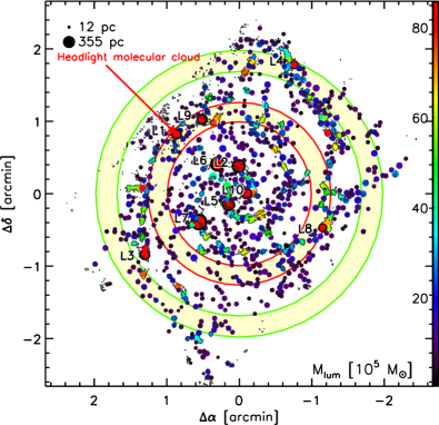
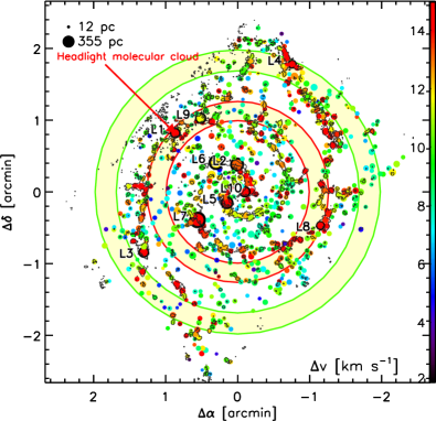
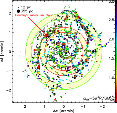
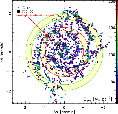
Figure 11: Position of molecular clouds in NGC 628. From top-left to bottom-right, colors correspond to the CO luminous masses, CO velocity linewidth, alpha virial parameter, and gas surface density, truncated to 8.6$\times$10⁶ $\mathrm{M_{\odot}}$, 15 km s^-1, 3.0, and 200 $\mathrm{M_{\odot}}$ pc^-2, respectively. Sizes of each symbol represent the physical size of the molecular clouds. In each panel we have marked the headlight molecular cloud (L1). The ten most massive molecular clouds are highlighted bold. The light yellow areas mark the position of corotation regions at 3.2 kpc (red circles) and 5.1 kpc (green circles). Contours correspond to the 5$\sigma$ level of the CO(2$-$1) moment zero map. Offset positions are from the galactic center.

5.2 Relation to the spiral arms and radial inflows

Here we consider the particular properties and star formation activity of NGC 628’s headlight cloud in relation to the large-scale dynamical structure of the disk. Figure 11 shows the spatial distribution of GMCs in the Rosolowsky et al. (in prep.) catalog, using colour to represent the CO luminous mass, velocity dispersion, virial parameter and molecular gas surface density of the clouds. The size of the symbol corresponds to the cloud size. The shaded light yellow circles represent corotation radii of 3.2 kpc (red circles) and 5.1 kpc (green circles) (see text below, Cepa & Beckman, 1990; Fathi et al., 2007), with an uncertainty of 15%.

It is evident from Fig. 11 that, as suggested in the previous section, large, massive clouds in NGC 628, including the headlight cloud, are located preferentially in the two prominent, tightly wrapped, spatially extended spiral arms. This suggests that the pattern of gas flow along and through the spiral arms may be important for determining the growth, longevity and properties of these clouds. The gas response to the spiral pattern has already been studied in detail by Fathi et al. (2007). They applied the Tremaine-Weinberg method to the ionized gas kinematics to measure a pattern speed $\Omega_{\rm p}$ that is consistent with the corotation radius at 5.1 kpc identified earlier by Cepa & Beckman (1990). This cororation radius lies near the edge of our map (green circles in Fig. 11).

In the presence of a single spiral pattern, with a single corotation radius, all the clouds within our field-of-view, including the headlight, would interact with the spiral pattern on a timescale of $\tau_{\rm sp}=\pi/(\Omega-\Omega_{\rm p})$. This yields $\tau_{\rm sp}=140$ Myr at the location of the headlight cloud. However, from the detailed kinematic analysis of Fathi et al. (2007), we infer a second, inner corotation radius at $R\approx 65$″$=3.2$ kpc, very near the position of the headlight cloud. In this case, the headlight would remain essentially motionless with respect to the spiral pattern over its entire life, as discussed further below.

Following Wong et al. (2004), the second corotation can be inferred from the pattern in the coefficients of the harmonic decomposition of the line-of-sight velocity field measured by Fathi et al. (2007). We have sought to confirm this inner corotation radius using a new measurement of gravitational torques across NGC 628. We follow the method of Querejeta et al. (2016) and García-Burillo et al. (2005), which requires a map of the 2D stellar mass distribution to infer the underlying disk volume density and gravitational potential $\Phi$, and a map of the gas distribution to provide a record of the time-averaged position of the gas relative to the potential. We use the 3.6$\mu$m contaminant-cleaned map produced by S⁴G Pipeline 5 (Querejeta et al., 2015) for the former, adopting a global $M/L=0.6$ assuming a Chabrier IMF (Meidt et al., 2014). We use the ALMA map shown in the right panel of Fig. 1 to trace the gas mass distribution. Following García-Burillo et al. (2005), we measure the azimuthally-averaged radial torque profile as

$$\tau(R)=\frac{\int_{\theta}[N(x,y)(xF_{y}-yF_{x})]}{\int_{\theta}N(x,y)},$$ (5)

where $R$ and $x,y$ are the radial and Cartesian coordinates, $N(x,y)$ is the gas column density, and the gravitational forces are computed from the reconstructed potential $\Phi$ with $F_{x,y}=\nabla_{x,y}\Phi$. We then measure the differential mass flow rate as

$$\frac{d^{2}M(r)}{dRdt}=\tau(R)\frac{1}{L}\bigg{|}_{\theta}2\pi RN(x,y)|_{\theta},$$ (6)

assuming that the azimuthal average of the angular momentum is $L_{\theta}$=$RV_{\rm rot}$. The resulting profile of inflow driven by gravitational torques is shown in the Fig. 12. Overall, the torque experienced by the gas in NGC 628 undergoes several sign changes, including a crossing from negative to positive near $R=65$″$=3.2$ kpc, which marks the location of our inner corotation radius, CoR_in, and corresponds to the galactocentric radius of the headlight cloud.

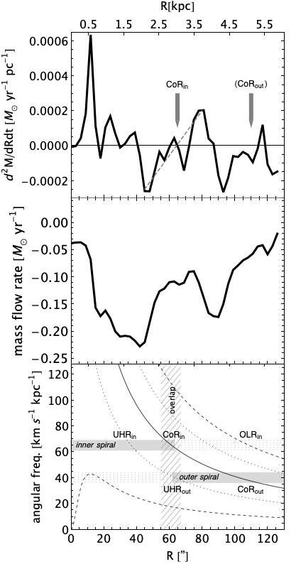
Figure 12: Top: Profile of differential gas flow $d^{2}M/dR\,dt$ driven by gravitational torques across NGC 628. The inner corotation radius (CoR_in) marked by an arrow is located where torques and gas flows cross from negative (inward) to positive (outward) as illustrated by the short dashed segment. The second arrow marks the position of the outer corotation radius, CoR_out, previously identified by Cepa & Beckman (1990), which falls near the edge of the CO field-of-view. Middle: Profile of integrated mass flow rates from the CoR_out inward to radius $R$. Net flows are radially inward (negative) at all radii. The uncertainty on the inflow (not shown) is dominated by the large, 15” uncertainty in the position of the CoR_out near the map edge. Bottom: Angular frequency curves in NGC 628, $\Omega$ (solid), $\Omega\pm\kappa/2$ (Dashed) and $\Omega\pm\kappa/4$ (Dotted). Positions of dynamical resonances and corotation radii are marked. The hashed vertical bar highlights the overlap between the CoR_in and the outer ultra-harmonic resonance.

The position of the headlight cloud very near the location of the inner corotation radius may have important implications for its longevity and ability to grow to its present mass, and thus the vigorous star formation occurring there. As indicated in the top panel of Fig. 12, gravitational torques and (differential) gas flows are zero at corotation. Thus, compared to other locations along the gaseous spiral arms, corotation is a relatively sheltered environment: a cloud at corotation radius is less susceptible to destructive dynamical forces such as shear, and rotates together with the spiral pattern during its entire evolution (i.e. $t_{\rm sp}\gg t_{\rm orb}$). Another factor that may promote the growth of the headlight cloud is that NGC 628’s inner corotation radius overlaps with one of the inner ultra-harmonic resonances (UHR) of the outer spiral pattern UHR_out, as illustrated in the bottom panel Fig. 12. In this case, gas sitting in the outer disk that is torqued by the outer spiral would be driven radially inward from the outer corotation radius, CoR_out, towards the UHR_out, providing a continual supply of gas to this region around CoR_in. Following Querejeta et al. (2016), we use the profile of gravitational torques to measure the radial flow across the disk of NGC 628, which we show in the middle panel of Fig. 12. From the measured $d^{2}M/dt\,dR$, we estimate that the net mass flow between the inner and outer corotation radius is indeed radially inward, at a net rate $0.07\pm 0.04$ $\mathrm{M_{\odot}}$ yr^-1. The inflow rate is a lower limit since it does not take into account a contribution from viscous torques (which are expected to be dominated by gravity torques; Combes et al., 1990; Barnes & Hernquist, 1996). We develop these ideas as a possible explanation for the mass growth of the headlight cloud in Section 6.3.

6 Discussion

We have identified the most luminous molecular cloud in NGC 628, the headlight cloud, which is $\sim 2.4$ times brighter in CO(2$-$1) than any other molecular cloud in NGC 628. It is the most massive cloud $(M_{\rm lum}=2.0\times 10^{7}\,\mathrm{M_{\odot}})$ in NGC 628. The cloud is located in a spiral arm at a galactocentric radius of $\sim 3.2$ kpc, which is coincident with a spiral corotation radius. The cloud itself hosts the most luminous H ii region in NGC 628 detected by MUSE, which is associated with a young ($2-4$ Myr) massive ($3\times 10^{5}$ $\mathrm{M_{\odot}}$) stellar population.

6.1 Overluminous CO emission in the headlight cloud

The central CO(2$-$1) integrated intensity and peak brightness temperature of the headlight cloud are high compared to the other GMCs in NGC 628, including other massive clouds. While a large integrated intensity could be due to a large cloud linewidth, Fig. 1 shows that the headlight cloud’s peak temperature is also $\sim 2$ times greater than other clouds in NGC 628.

More quantitatively, at the $\sim 40$ pc resolution of our CO(2$-$1) data, the average peak brightness temperature of the CO(2$-$1) emission from clouds with $M_{\rm vir}\geq 10^{6}$ $\mathrm{M_{\odot}}$ in NGC 628 is $T_{\mathrm{mb}}=1.3$ K. The headlight cloud peak temperature is 6.7 K. Making a local thermodynamic equilibrium simulation of the radiative transfer, which assumes that the headlight cloud is composed of “standard” molecular gas (i.e., with the characteristic kinetic temperature of 10 K, Krumholz 2011, e.g.) filling the full cloud volume, the predicted peak temperature would only be 5.5 K, i.e., less than the measured one. Alternatively, a typical kinetic temperature of 50 K would be required so that the headlight cloud has the same beam filling factor of a typical GMC of $10^{6}$ $\mathrm{M_{\odot}}$ in NGC 628. Hence, although our measurements do not exclude that there may be an additional increase in the filling factor of the CO(2$-$1) emission in the headlight cloud region, we favor an increase of the excitation temperature above 10 K to explain the headlight cloud’s peak brightness because of the spatial coincidence with the HII region heating source.

Another clue that heating is important comes from the CO(2$-$1)/CO(1$-$0) ratio, which we measured on 140 pc scales for the cloud population in NGC 628 in Fig. 7. This ratio is $\sim$0.7 in the headlight cloud, higher than the average ratio for the other bright clouds in Table 2 (0.6), and higher than the average ratio for the overall cloud population (0.54). One possibility is that intense external heating could cause a positive temperature gradient across the photospheres of CO-emitting clumps within the headlight cloud. Due to its larger opacity, the CO(2$-$1) transition might then preferentially sample a warmer clump layer than the CO(1$-$0) transition, raising the CO(2$-$1)/CO(1$-$0) ratio. We defer a more detailed investigation of the physical factors linked to variations in the CO(2$-$1)/CO(1$-$0) ratio in the disks of PHANGS galaxies to a future paper.

Almost all of the luminous GMCs in NGC 628 listed in Table 2, including the headlight cloud, have low virial parameters (see Fig. 3) as determined from the ratio between their CO luminosity and the virial mass estimates. If the CO(2$-$1) line is over-luminous due to excitation effects, then the true mass of the headlight cloud is smaller than the luminous mass estimate of $2.0\times 10^{7}$ $\mathrm{M_{\odot}}$. The low virial parameter and bright CO(2$-$1) emission in the headlight cloud is thus consistent with the suggestion by Pety et al. (2017) that mass estimates based on the CO luminosity may be biased when GMCs are closely associated with H$\alpha$ regions, as observed for the Milky Way Orion B cloud. If so, then clouds associated with H ii regions should show lower apparent virial parameters than otherwise identical clouds without nearby heating sources. We intend to test this hypothesis in a forthcoming paper using the full sample of PHANGS targets with cloud-scale imaging by ALMA and MUSE.

6.2 Feedback-limited lifetimes of clouds & prolonged survival of the most massive objects

The intense feedback from the newly-formed embedded stellar population in the headlight cloud is expected to lead to its eventual destruction. We appear to be observing the headlight cloud just before being destroyed by the feedback from the present generation of stars. In the simulations of Kim et al. (2018, see also ), massive clouds with higher escape velocities can withstand destruction via photoionization and radiative pressure longer than their lower mass counterparts. For a cloud with the headlight’s properties, $t_{\mathrm{dest}}\sim 10\,$Myr (Kim et al., 2018), which is longer than the age of the headlight’s young stellar population. If clouds with larger masses are able to survive for longer in the presence of feedback, then the overluminous state of the headlight cloud is linked not only to its star formation activity, but also to its large mass.

6.3 The influence of galaxy dynamics on cloud growth

If the mass of the headlight cloud is key to its longer survival time in the presence of feedback from star formation, the next question is what mechanism(s) allowed it to grow to its extraordinary mass. The dynamical environment of the headlight offers some clues.

Massive cloud formation and incipient starbursts are often linked to extreme conditions, such as in galaxy centers, at the ends of bars and in mergers (e.g. Kenney & Lord, 1991; Elmegreen, 1994; Böker et al., 2008; Kennicutt, 1998; Kormendy & Kennicutt, 2004; Elmegreen, 2011; Beuther et al., 2017), where elevated pressures can confine highly turbulent star-forming gas (e.g. Herrera & Boulanger, 2017; Johnson et al., 2015; Leroy et al., 2018). The normal disk environment may also provide a less extreme avenue for massive cloud growth (Meidt & Kruijssen, in prep.). As suggested earlier in Sect. 5.2, the spiral corotation radius where the headlight is positioned may furnish a favorable environment for the growth of particularly massive clouds.

At the corotation radius of a spiral pattern, the pattern moves at the same velocity as material in the galaxy disk. An individual cloud at the intersection of a spiral arm with a corotation radius will thus reside within the spiral pattern for its entire life. Here, gas experiences no gravitational torques and shear is locally reduced, promoting the longevity (and growth) of molecular clouds situated in this zone in the absence of feedback. In Section 5.2, we suggested that the headlight cloud’s position at the inner corotation radius may further support the mass growth of the cloud via gas flows driven into the region by gravitational torques. Normally, an isolated corotation radius is expected to be relatively devoid of gas (Elmegreen et al., 1996), due to the inflow (outflow) of material radially inward (outward) from this point (e.g. Garcia-Burillo et al., 1994; Meidt et al., 2013; Querejeta et al., 2015). However, NGC 628’s inner corotation radius appears to coincide with an inner dynamical resonance of the outer, independently rotating, spiral pattern (see bottom panel of Fig. 12). This type of scenario has been identified in simulations (Tagger et al., 1987; Rautiainen & Salo, 1999) and observations (Elmegreen et al., 2002; Meidt et al., 2009; Font et al., 2019). In this case, the radial inflow of gas possible from the outer corotation radius inward towards the inner corotation radius provides a potential mass reservoir for the cloud’s exceptional growth (Meidt & Kruijssen, in prep), raising its mass above the fiducial level set by competition between self-gravity, shear and feedback (e.g., Reina-Campos & Kruijssen, 2017).

We can use the mass inflow rate measured in Section 5.2 to estimate the timescale for the growth of the headlight cloud. On one hand, we can place a lower bound on this timescale, assuming that all of the material inflowing from the outer corotation radius is accreted onto it. The measured inflow rate in this case implies that the cloud grew to its present mass in time $t_{\rm grow}\sim 215\pm 100\,$Myr, which is roughly two orbital periods at the cloud’s location. On the other hand, considering that the inflow of gas onto the cloud is happening on multiple scales, this estimate can be viewed as an upper limit on the true growth timescale. Indeed, the mechanisms by which that matter accretes onto the cloud (e.g. turbulent or gravitationally-driven accretion, Ibáñez-Mejía et al., 2017) may incorporate local material that does not originate in the outer disk, allowing condensation to proceed much more rapidly. Viscous torques would also imply a shorter growth timescale, by increasing the mass inflow rate to the region.

7 Conclusions

We have presented a detailed study of the molecular line emission and star formation activity associated with the headlight cloud. This cloud is the most massive molecular cloud in NGC 628, and it hosts an exceptionally bright H ii region identified by MUSE (Kreckel et al., 2018). Our objective was to characterize the properties of this molecular cloud in the context of the internal (feedback) and external (dynamical) factors that may influence its formation and evolution.

Our main science results are:

• The headlight is 2.4 times brighter than any other cloud in CO(2$-$1), and it is the only source with HCO⁺(1$-$0), HCN(1$-$0) and HNC(1$-$0) emission detected by the ALMA 12-m array. The cloud is associated with the most luminous H ii region in NGC 628.

• The headlight cloud is the most massive ($M_{\rm lum}=2.0\times 10^{7}$ $\mathrm{M_{\odot}}$) cloud in NGC 628. Its virial parameter is low, $\alpha_{\rm vir}=0.5$. We argue that the CO emission is over-luminous based on its high CO(2$-$1) peak temperature and its spatial coincidence with a bright peak in the H$\alpha$ emission. This implies that its true molecular mass would be located between its virial mass of $9\times 10^{6}$ $\mathrm{M_{\odot}}$ and its luminous mass, $M_{\rm lum}$.

• According to a simple LVG analysis of the multi-line ALMA data, the typical density and temperature in the headlight cloud is $n_{\rm H_{2}}\sim 5\times 10^{4}$ cm^-3 and $T_{\rm kin}\sim 20$ K.

• From the presence of Wolf-Rayet features in the MUSE spectrum and modelling of the H$\alpha$ emission using Starburst99, we infer the presence of a young (2$-$4 Myr), massive ($3\times 10^{5}$ $\mathrm{M_{\odot}}$) stellar population that is still embedded inside the headlight cloud.

• We propose that feedback from the vigorous star formation happening within the headlight is responsible for its apparent overluminous state, captured just prior to the destruction of the cloud. This is possible given the longer survival times expected for the most massive objects (e.g., Kim et al., 2018).

• We propose that the extreme headlight mass within the NGC 628 disk is related to the large scale dynamics of the galaxy. In particular, the cloud’s location at the intersection of a spiral arm and the inner corotation radius implies not only a special location against the disruptive effects of galactic shear, but also a sustained inflow of gas favorable to enhanced mass growth. This scenario, in which clouds can grow to exceptional masses outside more prototypical ‘extreme’ environments, will be discussed in more detail in a future paper by Meidt & Kruijssen (in prep).

The exceptional star-forming activity and physical properties of the headlight cloud call for deeper, higher angular resolution ALMA observations of tracers of the molecular gas density distribution within the cloud.

In addition to our scientific results, we developed our own CASA data reduction procedures for the ALMA Total Power data in order to produce the position-position-velocity cube combining the ALMA 12m, 7m, and total power observations of NGC 628. These procedures, which are used in the reduction of all the Total Power data obtained by observational programmes led by the PHANGS consortium (e.g., Leroy et al., in prep.), are described in Appendix A. As part of our PHANGS-ALMA Large Programme commitments, the procedures have been transferred to the Joint ALMA Observatory so that they can be adapted for general use. Scripts implementing our procedures are also available on GitHub at https://sites.google.com/view/phangs/home/data.

Appendix A Total power data reduction

We have developed a set of customized scripts to carry out ALMA single dish (“total power” or TP) data reduction. These scripts play a crucial role in the PHANGS-ALMA reduction pipeline as the short-spacings often contain a significant fraction of the flux of nearby galaxies. They are based on the ALMA calibration scripts, with modifications informed by our experience carrying out and supporting single dish data reduction using the GILDAS software for IRAM 30-m data. The main aim of the scripts is to allow the user to define a fixed velocity window for the baseline subtraction while also producing a suite of diagnostic plots that allow assessment of imaging quality. This Appendix describes the structure and usage of these scripts.

The scripts have been provided to the ALMA Regional Centers and the Joint ALMA Observatory, where they have helped inform development of the Observatory data reduction scheme. They are available on GitHub at https://sites.google.com/view/phangs/home/data.

They were developed to be used in CASA version 4.7.2 that used the ASAP (ATNF Spectral Analysis Package) extension to deal with Total Power gridding and baselining. Since then, newer versions of CASA contain dedicated tasks that performs these tasks. We did not port our scripts yet.

The script distribution contains three files.

analysis_scripts

ALMA-provided folder that contains useful tools for TP ALMA data reduction. The scripts in this folder should not be modified.

ALMA-TP-tools.py

Script which contains our generic procedures for total power data reduction and imaging. This script should not be modified.

galaxy-specific-scripts

Folder containing the individual galaxy-specific scripts, GalaxyName-input.py, which are a wrapper for the two previous scripts. Here the user specifies various galaxy- and project-specific imaging parameters, including phase center position, source systemic velocity, rest frequency, channel width, final cube velocity width, and the definition of baseline subtraction windows (see additional details in the end-to-end reduction description below).

The distributed code has to be saved in a folder named scripts_TP folder. The galaxy-specific GalaxyName-input.py CASA script should be executed in this folder. Two additional folders will be created at the same level as the scripts_TP one, data and tmp. The first will contain the output cube fits files. The second is a temporary folder where the TP data reduction happens and intermediate files are stored. Once the data reduction is done, this folder can be deleted. Total Power raw data stored in the original ALMA directory structure are first replica in the tmp folder. Only the needed files are copied. Data reduction products are created in the calibration folder. Specifically, two additional subfolders are created, plots and obs_lists. The plots folder contains all plots created by the data reduction scripts, for example the $T_{\rm sys}$ and the baseline correction plots. The quality of the data can be judged checking these plots. The obs_lists folder contains the observation lists for the data.

The main script, ALMA-TP-tools.py, contains the procedures and tasks for the data reduction. We now describe the main steps in order of their execution during the processing.

Import data to MS and split by antenna

The raw ALMA data are stored in the Archival Science Data Model (ASDM) format. The data are converted to measurement sets (MS), a CASA table format, using the task importasdm. Initial flagging is applied with the task flagcmd. These are a priori flags, which are already encoded in and read from the MSs themselves. These flags could include issues such as when the mount is off source, calibration device is in an incorrect position, or power levels are not optimized. We also flag 7m antennas that may have been used for Total Power observations. Using the task sdsave, each execution block data set in the MS format is split by antenna and converted to the ASAP format.

Generate $T_{\rm sys}$ calibration tables and apply additional flags

For each ASAP file, a system temperature ($T_{\rm sys}$) calibration table is generated using the task gencal, which is needed to apply the calibration scale to the observations. One $T_{\rm sys}$ solution is created per spectral window. In this step, additional flagging to the data can also be applied by creating a script containing custom flag commands. This script should be placed in the galaxy-specific-scripts/flags-folder folder.

Subtract the atmospheric total power and convert to Kelvin

The $T_{\rm sys}$ calibration solution is applied to the data with the task sdcal2. At the same time, this task subtract the contribution of the atmosphere to the total power (subtraction of the OFF measurement) and it corrects for the chromatic response of the atmosphere and the receivers by dividing by the OFF measurement. The output will thus be expressed in units of antenna temperature as

$$T_{\rm a}^{\star}=T_{\rm sys}\times\frac{(\mathrm{ON}-\mathrm{OFF})}{\mathrm{OFF}}.$$ (7)

Extract the frequency window that contains the emission line

From this step on-wards, we choose to continue the data processing only for the spectral window that contains the emission line of interest plus a baseline margin on each side of the line. The user must define in the script GalaxyName-input.py both the rest frequency of the emission line and the velocity range of the cube that will be extracted from the data. The systemic velocity of the source is read from the MS. As the ALMA data are originally observed in the TOPO frame, the spectral axis is converted to the LSRK velocity frame at this stage to simplify the extraction. This uses functionality inside the analysis_scripts folder. The extraction of the cube is done with the task sdsave.

Baseline the spectra

We fit a polynomial though the spectrum parts that belong to the velocity ranges on both side of the lines. The velocity range to be ignored in this baseline fitting is defined in the GalaxyName-input.py script. More than one velocity window can be defined. The order of the baseline fit is one (i.e., a linear fit) by default, but this can also be changed in the GalaxyName-input.py script. Baseline fitting and subtraction call the the sdbaseline task.

Convert to Jy/Beam and concatenate data from all antennas

After all the above steps for data calibration are done, the ASAP files for all execution blocks and antenna are converted back to MS format using the task sdsave. For each execution block and individual antenna, the data are converted from Kelvin to Jansky using the factor measured and delivered by ALMA based on independent observations of point sources of known flux. This makes an higher order correction to the flux scale. All the data are then concatenated using the task concat.

Grid the spectra onto a pixelized cube

All the execution blocks together are imaged together. The user can define the imaging parameters such as the projection center, the velocity frame of refence, the total velocity width, and the channel width in the GalaxyName-input.py script. The gridding is done using the sdimaging task, in the LSRK velocity reference frame using a spheroidal function.

Export the position-position-velocity to a fits file

The task exportfits is used to export the signal and weight cubes to fits files.

In a few cases, an ozone telluric line were not satisfactorily subtracted during the ON-OFF processing because the atmosphere contribution to the total power varied too quickly. We used advanced baselining functionality in the GILDAS/CLASS software to remove this artifact and to obtain flat baselines. A deeper analysis that will be presented elsewhere (Usero et al., in prep) showed that a change of observing mode is sometimes required to get rid or at least decrease the contribution from some ozone lines.

Appendix B Headlight spatial distributions of multiple tracers

Figure 13: Peak temperature for the different gas tracers observed with ALMA. The bottom left inserts of each panel show the size of the synthesized beam. Colorbars are in units of K. White/black contours in the first/other panels, respectively, correspond to the 20%, 40%, 70% and 90% of the CO(2$-$1) peak temperature. The top-left panel shows in a black ellipse the headlight cloud as identified by CPROPS. Offsets positions are from the galactic center.

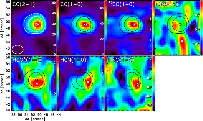
Figure 14: Integrated emission line for the different gas tracers observed with ALMA, convolved to the spatial resolution of ¹³CO(1$-$0).The bottom left inserts in the first panel shows the size of the synthesized beam. Emission for all tracers is integrated between 650 and 685 km s^-1, colorbars are in units of K km s^-1. White/black contours in the first/other panels, respectively, correspond to 15$\sigma$, 25$\sigma$, 50$\sigma$ and 100$\sigma$, with $\sigma$= 1.01 K km s^-1 of the CO(2$-$1) line. Offsets positions are from the galactic center.

Figure 13 shows the spatial distribution at full angular resolution of the peak brightness temperature around the headlight for the observed molecular lines: CO(2$-$1), CO(1$-$0), ¹³CO(1$-$0), CS(5$-$4), HCO⁺(1$-$0), HCN(1$-$0), and HNC(1$-$0). Figure 14 shows the spatial distribution of the emission integrated over the line profiles for the same tracers, after convolution to the worst angular resolution obtained, i.e., the ¹³CO(1$-$0). These figures shows that HCO⁺(1$-$0), HCN(1$-$0), and HNC(1$-$0) are clearly detected in contrast with CS(5$-$4). The high density tracers are slightly offset compared to the CO isotopologue lines. The relatively low signal-to-noise of the HCO⁺, HCN, and HNC lines makes the origin of the offsets uncertain.