In the present study, we developed algorithms that are capable of measuring apparent magnitudes and the effective temperature of stars using raw images shot with amateur telescopes. The regularized Radial Basis Function (RBF) network, one of the machine learning algorithms, was employed to measure the effective temperature, and the simple function fitting method was adopted to measure the apparent magnitude. The achieved results are satisfying. After the white balance and noise cancellation process was simply calibrated, it was demonstrated that the measurements of the effective temperature had mean fraction errors at around 9%, and the measurements of the magnitudes had absolute error at nearly 0.1.

$Key\ words:$ apparent magnitude, effective temperature, machine learning,regularized RBF network, amateur telescopes

1. Introduction

By measuring stellar apparent magnitudes and effective temperatures, multiple properties of stars can be more effectively revealed, covering their distance to the earth. In the current digital era, magnitudes are mostly measured using charged couple device (CCD) and professional telescopes in observatories. A commonly employed color index B-V (i.e., the difference between B band magnitude and V band magnitude) to measure the effective temperature of stars is also measured with specialized UBV filters that are mounted on observatory telescopes (Johnson & Morgan, 1953).

Though the measurements of apparent magnitude and color indices have long been mature, most measurements are dependent of either equipment specialized in observatories (e.g., UBV filters) or costly equipment inaccessible to amateur astronomers (e.g., CCDs). The reliance on specialized equipment has compelling reasons, and the reasons are high noise of non-cooled complementary-oxide-semiconductor (CMOS) used in ordinary cameras at high ISO, and their nonlinear response to the intensity of received light (Yadid-Pecht 1999). Thus, under an algorithm used to measure magnitudes and effective temperatures which is of relatively low dependence on data from professional equipment, part of amateur astronomers can facilitate sky surveys.

The rest of this paper is organized as follows. In section 2, the amateur telescope and camera, as well as star catalogue applied in this study to acquire labelled data are discussed. In section 3, the procedures of our observation and data reduction are illustrated, which covers white balance calibration, flat field correction, as well as noise cancellation. In section 4, the function fitting employed for magnitudes measurement are analyzed, and its accuracy and compatibility are delved into. In section 5, the ensemble learning algorithm is presented based on the regularized RBF network we adopted to measure the effective temperature. In section 6, the function developed by function fitting is presented, and the accuracy and compatibility of our measurement of the apparent magnitude and the effective temperature are discussed. Lastly, in section 7, all the results of this study are summarized, and the further improvement of the study is suggested based on the analysis of causes for abnormal errors.

2. Relevant Apparatus and Data Source

2.1. Canon 6Dmk2 and 200mm Cassegrain reflector

Canon 6Dmk2 refers to an ordinary digital single lens reflex (DSLR) with a full-frame CMOS. Given that the algorithms applied in this study for measuring the magnitude and the effective temperature is largely dependent of the CMOS adopted, Canon 6Dmk2 was taken as a popular ordinary camera that is used by numerous amateur astronomers.

The telescope applied here is a hyperbolic Cassegrain reflector, 200mm in aperture diameter and 1600mm in focal length. For the design of the pure reflector, the telescope exhibits no color aberration theoretically, so it is suitable for this study that highly depends on the color of stars; thus, the critical information about the effective temperature is reflected. As the target stars taken in this study display zenith distance $z<70^{\circ}$, the effects on the observed magnitude of the stars caused by atmospheric extinction (Karttunen et al. 2017) is defined as

$$\delta m=ksec\ z$$

Accordingly, the maximum difference in $\delta m$ of two stars with maximum separation in the field of view $dz\approx 1^{\prime}30^{\prime\prime}$ at $z<70^{\circ}$ is assessed as

$$d\delta m=\frac{ksinz}{cos^{2}z}\cdot dz<4\times 10^{-3}k$$

As a result, the atmospheric extinction is considered uniform within the small field of view of the telescope.

2.2. Gaia Sky Survey Data

BP magnitude ($m_{BP}$) and effective temperature ($T_{eff}$) from Gaia’s Data Release 2 (Gaia DR2) (Brown et al. 2018) were employed as the expected output. $m_{BP}$ was taken as the expected output of the sum of R,G,B readings in our images since ordinary cameras (e.g., 6Dmk2) has IR infra-red (IR) and ultra-violet (UV) filters; thus, the light could be approximately received within the wave band that is almost identical to that of $m_{BP}$, which is 330-680nm (Brown et al., 2018). Gaia DR2 was selected as it contains data for considerable number of stars between 14^th mag. and 16^th mag., and the stars we shot for labelled data largely met this range of magnitude. Every star in our images was matched with the star map and then labelled with the corresponding expected output from Gaia DR2.

3. Observations and Data Reduction

3.1. Observations

To shoot the images for labelled data, we went to Dunhuang, Gansu Province, a city near the desert in northwestern China, where the levels of light pollution are relatively low in China. To calibrate the sky-area we were shooting, the stars brighter than 2^th mag. were taken as centers of our images. Lastly, stars were used in the two images centering HIP65474 (Spica) and HIP67301 (Alkaid) as our labelled data source. The telescope was pointed to the selected stars and exposed for 30$s$ at 3200 ISO to create images that cover nearly 200 stars brighter than 16^th mag. surrounding the central calibration stars. The exposure parameters were adopted to ensure the sufficient number (about 200) of stars in each image as well as the acceptable amount of noise. Given the necessity to take multiple dark fields in astronomical researches, we still decided to leave noise cancellation process to algorithms. As we came to realize that amateur astronomers might not take dark fields when they were observing, the dark field involved into our research might reduce the compatibility of our algorithms. Flat fields were taken because they are unreplaceable by algorithms.

3.2. Data Reduction

3.2.1. White Balance Calibration

Since amateur astronomers are likely to exploit variable white balance setting in their cameras, the white balance of all the images and flat fields should be unified in the beginning. In practice, images in CR2/ RAW format are hard to adjust, while the use of other adjustable formats may result in a loss of information. Thus, the color temperature of the images were calibrated by the following algorithm.

$$g_{R}=\frac{\overline{R_{2}}}{\overline{R_{1}}},\ g_{G}=\frac{\overline{G_{2}}}{\overline{G_{1}}},\ g_{B}=\frac{\overline{B_{2}}}{\overline{B_{1}}}$$

We first outputted each raw image that was not adjusted as tif₁. Subsequently, the color temperature of the raw image was adjusted to $5770K$ and outputted as tif₂. The mean value of R channel reading of all the pixels in tif₁ was obtained as $\overline{R_{1}}$, and likewise for G and B channel, respectively. Next, by the mentioned formula, the mean value of R channel reading of all the pixels in the tif₂ was calculated as $\overline{R_{2}}$, and the gain on R channel as $g_{R}$; likewise, $g_{G}$ and $g_{B}$ were calculated.

$$R_{w}=R_{raw}\cdot g_{R},\ G_{w}=G_{raw}\cdot g_{G},\ B_{w}=B_{raw}\cdot g_{B}$$

Finally, with the mentioned formula, we obtained the white-balance-calibrated R channel reading of each pixel in the raw image $R_{w}$ , and likewise for $G_{w}$ and $B_{w}$ (Fig. 1). This specific color temperature was used as the most widely acknowledged “normal” white is defined by the spectrum of an approximately 5770K black body (Philips 1995). With this algorithm, both the images of stars as labelled data and flat fields were calibrated.

Figure 1: un-calibrated raw image (left) and white-balance calibrated image of HIP69672. Though this image did not finally act as labelled data for fewer stars in it, with its relatively low original color temperature, the effect on the white balance calibration could be more evidently shown.

3.2.2. Flat Field Correction

After white balance was calibrated for both stars and flat fields images, all the flat fields are averaged. Then, the common procedures was adopted to use flat field to eliminate the spatial non-uniformity of the CMOS caused by the entire imaging system. The R,G,B channel reading of each pixel in the image of stars after correcting the flat field are denoted as $R_{f},\ G_{f},\ B_{f}$, and R,G,B reading of the corresponding pixels in the averaged flat field are denoted as $R_{ff},\ G_{ff},\ B_{ff}$.

$$R_{f}=\frac{R_{w}\overline{R_{ff}}}{R_{ff}},\ G_{f}=\frac{G_{w}\overline{G_{ff}}}{G_{ff}},\ B_{f}=\frac{B_{w}\overline{B_{ff}}}{B_{ff}}$$

where $R_{w},\ G_{w},\ B_{w}$ denote the R,G,B channel reading of pixels in the white-balance-calibrated images, and $\overline{R_{ff}},\ \overline{G_{ff}},\ \overline{B_{ff}}$ indicate the mean value in R,G,B channels of all the pixels in the averaged flat field.

3.2.3. Noise Cancellation

Figure 2: After correcting the flat field, we cropped the image into “star patches” each sizing nearly 20$\times$20 pixels and containing a star respectively; a similar size of “background patch” was selected from the region surrounding each star patch correspondingly. A star patch and its background patch are presented in the lower red box and the upper red box, respectively.

After correcting the flat field and cropping the image into patches (Fig. 2), to enhance the reliability of labelled data by up-regulating their signal to noise ratio (SNR), the mean noise was subtracted from the star patches. The mean noise of each star patch in each channel was calculated with its corresponding background patch as the mean value of reading in R,G,B channel of all the pixels in the background patch $\overline{N_{R}},\ \overline{N_{G}},\ \overline{N_{B}}$. Subsequently, the mean noise was subtracted,

$$R_{m}=R_{f}-\overline{N_{R}},\ G_{m}=G_{f}-\overline{N_{G}},\ B_{m}=B_{f}-\overline{N_{B}}$$

The pixels with negative readings in any of the three channels that appeared after the mean was subtracted were considered noises and then set to 0, while the positive ones were left intact. Next, according to multiple trials, the pixels were set to 0 in the star patch with readings in any of the three channels that were smaller than the upper quartile (75%) of those in the corresponding channel of the background patch. The choice of 75% preserved sufficient information of the stars and effectively canceled most noises in the star patches.

After the mentioned cancellation process, it was noticed that considerable bright heat noises appeared frequently at high ISO, which were still “isolated pixels” in the star patches (Fig. 3). Another algorithm was adopted to set all pixels with all of adjacent pixels on their left, right, above, and below having 0 readings to 0, respectively. Thus, the effect of these bright heat noise pixels was reduced.

After all the noise cancellation, based on the observed results, we still discarded 29 of the faint stars with R,G,B reading comparable to noises in image that centers HIP65474. Subsequently, we discarded stars fainter than 15.5^th mag. and some star patches with the sum of RGB readings over 50000, while used the rest 182 star patches for subsequent measurement. We aimed to remove all stars over-exposed (with either R,G,B reading over 255) by setting the upper threshold of 50000. The same procedure was implemented with the image centering HIP67301, and 145 star patches were kept. Finally, the reading of the pixels in the star patches was then summed channel by channel.

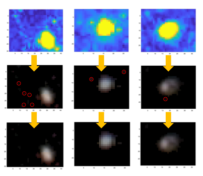
Figure 3: 3 star patches before noise cancellation, after mean noise and 75%th percentile noise were subtracted, and after “isolated pixels” were removed. The red circles marked the presence of “isolated pixels”

4. Measurement for Apparent Magnitude with Function Fitting

The apparent magnitude can be defined briefly as that the difference in magnitude of 5 indicates a 100 times proportion in intensities (greater value of magnitude corresponds to smaller intensity) (Carroll & Ostile 2014),

$$\frac{I_{1}}{I_{2}}=100^{(-\frac{m_{1}-m_{2}}{5})}\iff m_{1}-m_{2}=-2.5lg(\frac{I_{1}}{I_{2}})$$

where $I_{1},\ I_{2}$ denote the intensities of two stars, respectively, and $m_{1},\ m_{2}$ refer to their respective apparent magnitudes. As discussed above, two stars in one image exhibited roughly equal $\delta m$, so the mentioned equation still held with consideration of extinction. For CMOS, the $S=R+G+B$ of every star refers to a nonlinear function of intensity, so $m_{1}-m_{2}$ is a function about the natural logarithm of the ratio of $S$ of the two stars,

$$m_{1}-m_{2}=f(-lg(\frac{S_{1}}{S_{2}}))=f(-ln(\frac{S_{1}}{S_{2}})/ln10)=kf(-ln(\frac{S_{1}}{S_{2}}))$$

where $k$ is a constant, and $S_{1},\ S_{2}$ denote the sum of R,G,B of the two stars, respectively. Given the relation above, the application of function fitting is considered to be feasible.

One bright star (apparent magnitude around 10^th mag.) in one image that underwent the data reduction described above was taken as the reference star, and its RGB sum reading $S_{0}$ and expected output apparent magnitude $m_{0}$ were adopted for the reference. Based on the mentioned discussion, the measured magnitude $\hat{m}_{i}$ of a star with reading $S_{i}$ in the image can be yielded,

$$\hat{m}_{i}=f(dm_{i})+m_{0},\ dm_{i}=-ln(\frac{S_{i}}{S_{0}})$$

A strong logarithmic pattern was found according to the observed distribution of $\Delta m_{i}=m_{i}-m_{0}$ vs $dm_{i}=-ln(\frac{S_{i}}{S_{0}})$ where $S_{i}=R_{i}+G_{i}+B_{i}$ and $m_{i}$ is its corresponding expected output, both from each $i$th among the 181 “star patches” in the image centering HIP65474. Accordingly, the relation between $\Delta m_{i}$ and $dm_{i}$ was directly fitted by logarithm function,

$$\hat{m}_{i}=f(dm_{i})+m_{0}=aln(b\cdot dm_{i}+1)+m_{0}$$

where $a,\ b$ represent coefficients to be determined by the data. Using this method, the absolute error $a_{i}$ of our fitted function $f$ on any $i$th star patch was assessed,

$$a_{i}=|\hat{m}_{i}-m_{i}|$$

Several attempts were made, covering regularized RBF network and ensemble learning the result to fit the data, whereas a larger error was yielded.

5. Measurement of Effective Temperature with Regularized RBF Network and Ensemble Learning

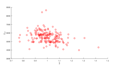
Figure 4: The scatter plot of $T_{eff}$ vs $\frac{G}{B}$ showed no apparent pattern between the two variables, so the attempt to find the 1-dimensional relation between the two variables was discarded.

The theoretical relation between $T_{eff}$ and R, G, B readings is evident. Similar to UBV color system, R,G,B readings reveal the intensity of radiation from the star collected on the R,G,B wave bands. Since the effective temperature is critical to the stars’ black body spectra, it can be ascertained with R and B readings as a two-variable function,

$$T_{eff}=F(R,B)$$

The specific choice of using R and B instead of the ratio of $\frac{G}{B}$ or R, G, B was made by multiple attempts. We have considered that the ratio $\frac{G}{B}$ corresponds to the ratio of intensity collected in the B and V band in UBV color system and therefore corresponds to the color index $B–V$, which is commonly used for determining effective temperature; however, no obvious pattern was displayed in the distribution of $T_{eff}$ with $\frac{G}{B}$ of our data (Fig. 4). In brief, it was found that adopting R and B as a set of 2-dimensional inputs of the unknown function to measure the effective temperature yielded the highest accuracy. Given the availability of relatively sufficient labelled data, machine learning was used in this study as it can potentially give an accurate estimation of the unknown function. Specifically, we used regularized Radial Basis Function (RBF) network, i.e., a machine learning algorithm, to measure the effective temperature.

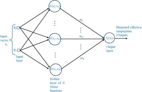
Figure 5: The regularized RBF network. Each approximating function $F_{j}(x_{i})=\sum\limits_{n=1}^{N}w_{n}G(x_{i},x_{n})$, where size of the training set $N$ equates number of labelled data. The expansion coefficients $w_{n}$ are determined based on the labelled data (Poggio & Girosi 1990).

We used a total of 145 labelled data from the image centering HIP67301 to train the RBF network to obtain $F(R,B)$. The labelled data were 2-dimensional vectors $x_{i}=(R_{i},\ B_{i}),\ i=1,\ 2,\ ...N$, and their corresponding expected output were $T_{eff_{i}},i=1,\ 2,\ ...,\ N$, where $N$ denotes the total number of labelled data (“star patches”) in the image. 80% of the labelled data were randomly sampled to train the regularized RBF network, and one approximating function $F_{j}$ that measures the effective temperature was outputted (Fig. 5). The process was repeated for 1000 times, so 1000 different approximating functions $F_{j},\ j=1,\ 2,\ ...1000$ were yielded. With the $1000\ F_{j}$ , ensemble learning was conducted to output the measured effective temperature $\hat{T}_{eff}$ (Fig. 6). At a given unknown input RGB vector $x$, the measurement of the effective temperature could be calculated,

$$\hat{T}_{eff}=\frac{\sum\limits_{j=1}^{1000}F_{j}(x)}{1000}$$

Figure 6: Measurement of the effective temperature with ensemble learning. The loss function of the regularized RBF network is defined as $L(F_{j})=L_{s}(F_{j})+\lambda L_{c}(F_{j})$, where the regularization parameter $\lambda=1\times 10^{-2}$, as calculated with the labelled data (Craven & Wahba 1979); $L_{s}(F_{j})=\frac{1}{2}\sum\limits_{i=1}^{N}(T_{eff_{i}}-F_{j}(x_{i})^{2})$ where $L_{s}(F_{j})$ indicates the standard loss function, $L_{c}(F_{j})=\frac{1}{2}||DF_{j}||^{2}$ where $L_{c}(F_{j})$ refers to the regularization term (Tikhonov 1963).

The generalization error of $\hat{T}_{eff}$ was assessed as below: for a specific labelled data $x_{i}$ and its corresponding expected output $T_{eff_{i}}$, there exist $k$ functions among the 1000 $F_{j}$s, with $x_{i}$ not included in their training sets, expressed as $F_{i1},F_{i2},...,F_{ik}$. We are able to calculate the generalization error of $\hat{T}_{eff}$ tested by respective $x_{i}$ (Fig. 7),

$$e_{i}=\frac{\sum\limits_{r=1}^{k}\frac{|F_{ir}(x_{i})-{T_{eff}}_{i}|}{{T_{eff}}_{i}}}{k}$$

Then, the mean generalization error of $\hat{T}_{eff}$ on all the labelled data is calculated,

$$E_{\hat{T}_{eff}}=\frac{\sum\limits_{i=1}^{N}e_{i}}{N}$$

In such a way, we have made use of every labelled data as testing data for once, hence improving the reliability of the generalization error and achieved higher utility of our limited data.

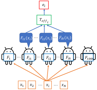
Figure 7: Calculation of generalization error $e_{i}$.

6. Results

6.1. Magnitude Measurement

Data from the 181 star patches in HIP65474 were adopted to perform the function fitting algorithm, and the function below was yielded to measure the apparent magnitude (Fig. 8),

$$\hat{m}_{i}=3.0907ln(0.7970\cdot ln(\frac{S_{i}}{S_{0}})+1)+m_{0}$$

Due to different atmospheric extinction effect on stars at various altitudes, we used data from HIP65474 solely.

Figure 8: The original distribution of $\Delta m$ vs $dm$ and the logarithmic function fitted $\hat{m}–m_{0}=f(dm)$ using the data from HIP65474.

To display the distribution of the absolute error of the function in measuring magnitude, we plotted the histogram with 10 classes (Fig. 9). The mean of all the absolute errors $a_{i}$ was calculated, which is 0.1035^thmag., and its 90% confidence interval, which is $0.1035\pm 0.0106^{th}$mag..

Figure 9: The histogram of $\hat{m}$ with absolute error $a_{i}$ with 10 equal classes of the 181 labelled from HIP 65474.

6.2. Effective Temperature Measurement

To measure the effective temperature, we employed labelled data from 145 “star patches” in the image centering HIP67301. The generalization errors in the measured $\hat{T}_{eff}$ concentrated on relatively smaller values (Fig. 10). Furthermore, despite some individual measured effective temperature with abnormally large errors, the mean generalization error $E_{\hat{T}_{eff}}$ exhibits 0.07 and 90% confidence interval of $e_{i}$ is $0.07\pm 0.01$.

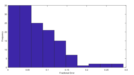
Figure 10: The histogram of generalization error $e_{i}$ with 10 equal classes of the 145 testing data from HIP 67301.

As $F(x),\ x=(R,B)$ depends on the relation between R and B, $\hat{T}_{eff}$ trained with one image can be adopted to measure with unknown data from another image. For verification, we measured the effective temperature with $x_{i}$ from image centering HIP65474 using $\hat{T}_{eff}$ function trained with data from HIP67301, and we yielded the mean generalization error of 0.09 and 90% confidence interval of $0.09\pm 0.01$ (Fig. 11).

Figure 11: The histogram of the fractional errors of $\hat{T}_{eff}$ with 10 classes. The function trained with data from HIP67301 are used to measure the effective temperature of the 181 stars in the image of HIP65474 with their R and B data.

7. Conclusions and Discussion

As discussed above, one algorithm was developed to measure the apparent magnitudes, while the other was yielded to measure the effective temperature with data from amateur telescopes. Our measurement of magnitudes exhibited absolute error at about 0.1 and measurement of the effective temperature displayed a mean generalization error at nearly 0.09. The algorithm for measuring effective temperature can be used on different images shot at the same geographic location and within a short period of time. Both algorithms are compatible with various white balances and do not require the use of dark fields.

It was reported that there exist a “v” shape distribution of the generalization errors and corresponding effective temperature (Fig.12), indicating $\hat{T}_{eff}$ is more inaccurate when the star has relatively lower ($<4750K$) or higher ($>6000K$) $T_{eff}$.

Figure 12: The distribution of generalization error vs expected output $T_{eff}$ with data from HIP67301.

We hypothesized that this “v” shape distribution of generalization error is caused by relative scarcity of labelled data with $T_{eff}<4750K$ and $T_{eff}>6000K$, which is supported by the distribution of labelled data (Fig. 13). As a result, the accuracy of $\hat{T}_{eff}$ can be enhanced when more labelled data that has $T_{eff}$ out of the interval [$4750K,\ 6000K$] are incorporated into future researches.

Figure 13: The histogram of expected output $T_{eff}$ with 10 classes in the image centering HIP67301.

Appendix

Table 1: Measurement of apparent magnitude with labelled data from the image centering HIP65474.

$S_{i}$	$m_{i}$	$\hat{m}$	$a_{i}$
25848	12.7519	12.6529	0.0990
16072	13.3279	13.3684	0.0405
5140	14.4830	14.6130	0.1300
3539	14.8210	14.9314	0.1104
9621	14.0388	13.9911	0.0477
5243	14.4920	14.5951	0.1031
11667	13.8626	13.7715	0.0911
7163	14.2754	14.2994	0.0240
4100	14.6483	14.8098	0.1615
18793	13.1382	13.1507	0.0125
13186	13.7395	13.6236	0.1159
4151	14.6898	14.7993	0.1095
23311	12.9359	12.8231	0.1128
29468	12.5652	12.4224	0.1428
5968	14.5850	14.4758	0.1092
11270	13.8006	13.8121	0.0115
16519	13.3493	13.3313	0.0180
16466	13.2809	13.3357	0.0548
2855	15.0680	15.1008	0.0328
5867	14.3746	14.4918	0.1172
7321	14.3572	14.2776	0.0796
16741	13.2359	13.3131	0.0772
25483	12.7253	12.6769	0.0484
12048	13.6310	13.7334	0.1024
6302	14.4590	14.4242	0.0348
22710	12.9790	12.8647	0.1143
2769	15.0464	15.1242	0.0778
2062	15.3386	15.3410	0.0024
8569	14.1080	14.1158	0.0078
3806	14.9188	14.8719	0.0469
5220	14.7628	14.5991	0.1637
6658	14.4685	14.3713	0.0972
3792	14.9802	14.8750	0.1052
7767	14.2840	14.2178	0.0662
2876	15.3652	15.0952	0.2700
5225	14.5280	14.5983	0.0703
23167	12.7274	12.8331	0.1057
25609	12.5920	12.6686	0.0766
15044	13.4711	13.4560	0.0151
9756	13.9126	13.9757	0.0631
4924	14.5889	14.6514	0.0625
4957	14.6884	14.6454	0.0430
3704	15.1164	14.8943	0.2221
13860	13.4588	13.5613	0.1025
5268	14.5480	14.5908	0.0428
2154	15.2350	15.3098	0.0748
44291	11.7953	11.5713	0.2240
10770	13.8737	13.8645	0.0092
15264	13.4524	13.4370	0.0154
30429	12.3908	12.3632	0.0276
5350	14.6925	14.5768	0.1157
19767	13.1549	13.0769	0.0780
4908	14.5760	14.6543	0.0783
2090	15.3456	15.3314	0.0142
19864	13.0804	13.0697	0.0107
2532	14.9653	15.1916	0.2263
3783	14.8093	14.8769	0.0676
7654	14.2354	14.2327	0.0027
13646	13.5844	13.5809	0.0035
9054	14.1613	14.0571	0.1042
8755	14.0189	14.0930	0.0741
7694	14.2095	14.2274	0.0179
7635	14.0994	14.2353	0.1359
3331	14.8234	14.9802	0.1568
11609	13.7085	13.7774	0.0689
2201	15.2360	15.2943	0.0583
8695	14.1207	14.1003	0.0204
6746	14.6704	14.3585	0.3119
3745	14.9629	14.8852	0.0777
4098	14.8217	14.8102	0.0115
4210	14.7260	14.7874	0.0614
3835	14.6832	14.8656	0.1824
2666	15.2739	15.1530	0.1209
18718	13.0360	13.1564	0.1204
4207	14.9007	14.7880	0.1127
6373	14.3767	14.4135	0.0368
2368	15.1673	15.2411	0.0738
1039	15.4993	15.7930	0.2937
7987	14.0153	14.1891	0.1738
1979	15.4943	15.3700	0.1243
6984	14.3862	14.3245	0.0617
5809	14.4568	14.5011	0.0443
2312	15.2783	15.2586	0.0197
1259	15.3369	15.6728	0.3359
3593	15.1298	14.9191	0.2107
3964	14.8469	14.8381	0.0088
12765	13.7130	13.6635	0.0495
9811	14.0405	13.9695	0.0710
5427	14.6045	14.5638	0.0407
7873	14.2779	14.2039	0.0740
1751	15.4557	15.4550	0.0007
3911	15.1281	14.8493	0.2788
2337	15.2036	15.2508	0.0472
9183	14.1234	14.0418	0.0816
6010	14.6864	14.4692	0.2172
4288	14.7873	14.7718	0.0155
4986	14.7559	14.6402	0.1157
30532	12.2316	12.3569	0.1253
11999	13.8636	13.7382	0.1254
2696	15.3618	15.1445	0.2173
11413	13.8811	13.7974	0.0837
11985	13.7635	13.7396	0.0239
20439	13.0408	13.0271	0.0137
8752	13.9100	14.0934	0.1834
5893	14.3396	14.4877	0.1481
5849	14.3770	14.4947	0.1177
5252	14.4217	14.5936	0.1719
5928	14.4789	14.4821	0.0032
4872	14.7160	14.6608	0.0552
3774	14.7898	14.8789	0.0891
8138	14.1559	14.1698	0.0139
3074	15.0296	15.0436	0.0140
6025	14.0915	14.4669	0.3754
3915	14.7300	14.8485	0.1185
12167	13.8138	13.7216	0.0922
27781	12.6636	12.5282	0.1354
4652	14.6886	14.7014	0.0128
6128	14.6102	14.4508	0.1594
3476	15.2395	14.9460	0.2935
12338	13.6838	13.7048	0.0210
13072	13.7412	13.6344	0.1068
2324	15.4334	15.2549	0.1785
28987	12.4511	12.4523	0.0012
3780	14.8555	14.8776	0.0221
2108	15.3559	15.3253	0.0306
12515	13.4950	13.6876	0.1926
4679	14.5797	14.6963	0.1166
2291	15.1068	15.2653	0.1585
33436	12.5045	12.1827	0.3218
9235	14.1145	14.0357	0.0788
5137	14.5448	14.6136	0.0688
10108	13.9240	13.9363	0.0123
36056	12.0838	12.0301	0.0537
3959	14.8872	14.8392	0.0480
34186	12.1736	12.1386	0.0350
34358	12.0319	12.1285	0.0966
31728	12.1266	12.2844	0.1578
5975	14.4593	14.4747	0.0154
4536	14.6600	14.7234	0.0634
3275	14.9791	14.9937	0.0146
4433	14.6373	14.7432	0.1059
6149	14.4671	14.4476	0.0195
8030	14.2280	14.1836	0.0444
10121	13.8412	13.9349	0.0937
7892	14.0501	14.2014	0.1513
16469	13.0848	13.3354	0.2506
4604	14.9887	14.7104	0.2783
10175	13.7093	13.9289	0.2196
15853	13.2100	13.3868	0.1768
16511	13.0593	13.3320	0.2727
4900	14.8488	14.6557	0.1931
3108	14.8956	15.0350	0.1394
4235	14.9564	14.7824	0.1740
2812	15.1193	15.1125	0.0068
19929	12.8762	13.0648	0.1886
12419	13.6861	13.6969	0.0108
2781	15.2080	15.1209	0.0871
33790	12.0710	12.1618	0.0908
7255	14.3494	14.2867	0.0627
4759	14.6110	14.6815	0.0705
5817	14.5363	14.4998	0.0365
9010	14.1731	14.0623	0.1108
16075	13.3508	13.3682	0.0174
4209	15.0816	14.7876	0.2940
14374	13.4471	13.5150	0.0679
8362	14.1853	14.1415	0.0438
25959	12.4494	12.6456	0.1962
15994	13.5760	13.3749	0.2011
11748	13.7758	13.7634	0.0124
27398	12.6873	12.5526	0.1347
5653	14.3732	14.5263	0.1531
15143	13.4274	13.4474	0.0200
9316	13.8082	14.0263	0.2181
27634	12.7848	12.5375	0.2473
36697	12.4733	11.9934	0.4799
15403	13.5678	13.4250	0.1428
28387	12.6146	12.4899	0.1247
45666	11.4969	11.4969	0.0000
9441	14.0328	14.0117	0.0211
6378	14.1172	14.4127	0.2955
23743	13.0053	12.7935	0.2118

Note. Column 1: sum of RGB $R_{i}+G_{i}+B_{i}$ from each star patch. Column 2: expected output of apparent magnitude. Column 3: measured magnitude. Column 4: absolute error of each measured magnitude.

Table 2: Measurement of effective temperature with labelled data from the image centering HIP67301.

$R_{i}$	$B_{i}$	${T_{eff}}_{i}$	$\hat{T}_{eff}$	$e_{i}$
9125	10902	5798.75	5721.25	0.01
12822	15273	6342.75	5977.76	0.06
2499	2100	4364.00	4638.79	0.06
1950	1692	5740.67	4750.22	0.20
3992	4281	5790.50	5476.52	0.05
8918	9046	5544.00	5342.71	0.04
1750	2120	5367.00	5576.43	0.04
2852	3411	5248.10	5630.44	0.07
1758	2142	4956.66	5604.32	0.13
10261	12247	5875.00	5530.61	0.06
3060	3562	4897.33	5584.26	0.14
3599	4448	5770.25	5753.18	0.00
7988	9992	5865.33	5944.31	0.01
1698	2258	5298.00	5809.36	0.10
3376	4264	6502.25	5740.16	0.12
8804	10547	5867.00	5754.42	0.02
2386	2321	4844.41	5021.76	0.04
9544	11405	5853.50	5638.23	0.04
2308	2834	5403.25	5647.26	0.05
5749	7278	5779.33	5682.16	0.02
5886	6762	5029.00	5731.04	0.14
6216	6837	5766.00	5661.00	0.02
974	1198	4973.67	5520.02	0.11
1782	2414	6138.00	5829.75	0.05
4569	5201	5363.00	5693.06	0.06
8676	10890	6272.00	5774.97	0.08
2116	2595	4957.75	5644.18	0.14
904	1099	5449.83	5461.44	0.00
2061	2388	5322.00	5479.82	0.03
1393	1362	5454.44	5134.83	0.06
6760	7305	5084.58	5704.90	0.12
6173	7793	5556.00	5760.21	0.04
3277	3619	5830.25	5437.34	0.07
6155	7662	5286.90	5794.34	0.10
4285	4349	5515.94	5419.68	0.02
4275	4392	5217.08	5475.33	0.05
2201	1502	4115.33	4248.81	0.03
8377	9008	5025.33	5637.60	0.12
898	1234	5332.00	5651.24	0.06
1680	2057	5710.75	5588.75	0.02
12620	15025	4986.31	6446.55	0.29
1328	1535	6171.61	5423.83	0.12
3566	4262	5811.75	5674.30	0.02
3968	4762	5112.29	5750.94	0.12
1574	1953	5880.67	5601.72	0.05
15600	17538	5037.70	5738.42	0.14
2590	3013	5663.00	5513.45	0.03
3405	3700	5245.11	5429.55	0.04
640	625	5037.70	5238.14	0.04
5221	6161	5810.25	5687.12	0.02
3638	4553	5836.00	5774.12	0.01
1805	2266	5335.11	5672.28	0.06
965	1144	5045.10	5459.85	0.08
3674	4431	5297.00	5731.00	0.08
794	1031	5601.65	5510.02	0.02
1247	1315	4912.80	5291.36	0.08
5401	6708	6297.00	5617.60	0.11
731	928	5971.15	5401.62	0.10
1283	1429	5635.25	5366.69	0.05
4171	5166	5786.00	5756.89	0.01
2358	2783	5805.25	5531.08	0.05
999	1452	5564.05	5785.92	0.04
10623	12219	5005.00	5624.99	0.12
14029	17051	6806.22	5804.88	0.15
1824	2013	4910.83	5369.84	0.09
4486	4620	5813.67	5477.84	0.06
2604	2963	5745.00	5446.51	0.05
2405	2333	5045.92	5007.53	0.01
15443	18055	5933.33	5394.39	0.09
2668	3236	5355.75	5648.02	0.05
1981	1481	4227.50	4513.31	0.07
1453	995	4190.64	4653.30	0.11
1569	1700	5502.91	5317.63	0.03
6856	7486	6138.00	5609.70	0.09
1444	1295	5312.00	4968.40	0.06
11578	12896	5783.25	5511.49	0.05
3766	3654	5811.25	5128.70	0.12
3881	3194	4947.05	4637.99	0.06
4150	4975	5831.33	5720.07	0.02
12323	12643	6362.00	5035.64	0.21
2487	3472	5925.30	5995.68	0.01
6809	6597	5803.00	5524.76	0.05
2438	2447	5347.75	5096.40	0.05
1669	1835	5112.47	5355.87	0.05
14903	14790	4999.64	5066.22	0.01
13002	14096	5858.00	5677.54	0.03
2843	3640	5782.75	5795.63	0.00
1476	1697	5515.04	5439.51	0.01
4975	5749	5004.00	5749.07	0.15
1811	1785	4911.89	5108.09	0.04
2674	2845	5136.00	5275.72	0.03
2673	2559	4344.79	4992.13	0.15
1496	1764	6451.00	5468.42	0.15
2372	2961	5479.50	5699.96	0.04
1516	1780	5087.00	5496.81	0.08
3203	3323	5676.00	5241.62	0.08
9957	10325	4898.66	5405.12	0.10
3693	4033	6256.00	5457.14	0.13
8665	8181	5626.00	5163.13	0.08
9652	10556	5777.25	5392.22	0.07
2454	2628	5440.24	5274.95	0.03
3189	3038	4665.58	5011.02	0.07
8502	8315	5408.33	5364.43	0.01
2092	2116	5144.33	5132.20	0.00
3146	3525	5568.28	5470.46	0.02
6303	6298	5131.81	5723.49	0.12
4688	4208	5409.00	5186.05	0.04
7723	8678	5120.75	5760.50	0.12
1233	1709	6395.75	5747.58	0.10
2241	1980	4458.00	4799.22	0.08
6431	6691	5755.00	5623.39	0.02
3718	4674	5480.29	5812.10	0.06
3710	4175	5094.67	5582.66	0.10
1632	2232	6752.50	5791.99	0.14
2353	2703	5421.33	5467.72	0.01
1220	1485	5012.04	5540.56	0.11
1465	1678	5992.11	5420.02	0.10
2251	2448	5294.05	5318.13	0.00
12130	12970	5575.18	5518.42	0.01
7110	8816	6322.67	5705.58	0.10
12670	13085	4945.94	5727.75	0.16
3030	3177	4938.30	5278.67	0.07
2923	2920	5148.85	5105.36	0.01
2442	3102	6197.00	5723.94	0.08
11442	13902	6321.00	5388.74	0.15
5530	6753	6342.67	5617.21	0.11
5100	5683	6214.00	5626.46	0.09
3213	3014	5752.00	4914.45	0.15
9727	11072	4783.59	5646.44	0.18
10807	12169	5015.69	5563.43	0.11
2502	2205	3914.55	4791.16	0.22
4007	4569	5115.33	5649.70	0.10
2557	3213	5939.75	5720.62	0.04
823	1134	5342.33	5626.37	0.05
1244	1295	6808.00	5203.39	0.24
2127	2051	5485.00	4999.34	0.09
2794	3663	5934.50	5848.22	0.01
7350	8097	5783.50	5644.71	0.02
1480	1986	5760.88	5766.89	0.00
1853	2556	6824.50	5843.81	0.14
1126	1387	5344.50	5533.68	0.04
1116	1510	4633.64	5732.42	0.24
9054	9625	5889.00	5389.13	0.08
3438	4073	5811.75	5645.95	0.03

Note. Column 1: the R channel reading from each star patch. Column 2: the B channel reading from each star patch. Column 3: expected output of effective temperature. Column 4: measured effective temperature. Column 5: generalization error tested on each labelled data.

Table 3: Measurement of effective temperature using unknown data in HIP65474 with the $\hat{T}_{eff}$ function obtained from data in HIP67301.

$R$	$B$	${T_{e}ff}_{i}$	$\hat{T}_{eff}$	$e_{i}$
8403	8730	6027.00	5490.99	0.09
5282	5277	6732.10	5581.39	0.17
2100	1514	5104.50	4376.25	0.14
1092	1127	5437.67	5251.24	0.03
3521	3018	4915.20	4733.16	0.04
1694	1760	5982.50	5226.25	0.13
5256	3003	4848.37	4140.71	0.15
2718	1965	3993.00	4204.19	0.05
1407	1439	4945.00	5219.45	0.06
6247	6148	5946.50	5615.23	0.06
4991	3961	4590.51	5016.51	0.09
1390	1325	5055.77	5100.24	0.01
8263	7216	5082.69	5284.54	0.04
11602	8565	4319.95	4286.58	0.01
2059	2079	4973.00	5131.51	0.03
3809	3669	4947.87	5166.48	0.04
5964	5211	4882.15	5489.41	0.12
5013	5712	6506.09	5691.02	0.13
1088	856	4937.00	4909.23	0.01
1890	1886	6044.50	5119.51	0.15
2286	2577	5593.85	5411.00	0.03
5413	5459	5483.25	5605.81	0.02
8597	8409	5761.00	5355.93	0.07
3782	4169	6310.00	5523.87	0.12
2330	1830	4857.14	4488.02	0.08
8517	6942	4971.09	5161.12	0.04
927	878	4947.62	5150.13	0.04
676	716	6449.00	5256.62	0.18
2907	2972	5879.00	5173.63	0.12
1603	1910	5382.75	5521.87	0.03
2165	2450	6603.50	5417.50	0.18
1360	1225	4943.00	5014.62	0.01
2685	2602	5467.02	5002.81	0.08
989	989	6541.00	5211.55	0.20
1764	1645	4969.00	4992.54	0.00
7328	8200	6554.00	5677.74	0.13
9589	7740	4452.64	4841.75	0.09
5318	4707	4830.40	5389.68	0.12
2987	3426	6744.00	5513.63	0.18
1499	1829	5427.00	5564.18	0.03
1683	1581	5004.00	5022.22	0.00
1165	1272	4980.33	5336.22	0.07
4384	4724	6413.00	5572.65	0.13
1820	1692	5759.66	4975.75	0.14
659	787	6020.40	5367.92	0.11
14611	14944	5718.60	5295.83	0.07
3661	3652	5854.00	5231.87	0.11
5323	5112	4949.00	5532.60	0.12
9937	10569	6318.50	5344.35	0.15
15525	17697	6302.00	5497.72	0.13
1940	1648	4428.74	4760.89	0.07
7049	6429	5085.45	5523.77	0.09
1497	1748	5796.00	5472.52	0.06
626	767	6045.33	5381.67	0.11
6514	6927	5965.67	5645.91	0.05
861	790	5327.00	5121.71	0.04
1464	1151	5428.33	4776.38	0.12
2938	2334	5627.97	4436.84	0.21
4801	4445	6043.75	5347.63	0.12
3370	2904	5381.95	4719.28	0.12
3024	2743	5949.50	4829.13	0.19
2775	2318	5261.00	4582.53	0.13
2689	2355	5773.67	4717.36	0.18
1092	1157	5770.00	5288.99	0.08
3841	3945	5954.00	5355.28	0.10
675	766	4429.50	5321.92	0.20
3092	2758	5044.00	4785.38	0.05
2214	2290	5939.61	5183.56	0.13
1401	1236	6302.06	4972.50	0.21
1396	1340	5869.00	5110.94	0.13
1374	1457	5744.00	5286.02	0.08
1058	1420	8427.67	5655.79	0.33
800	1003	6009.67	5469.40	0.09
5903	6213	5478.33	5654.75	0.03
1267	1478	8657.00	5454.03	0.37
1940	2186	5836.00	5403.12	0.07
675	875	5572.01	5460.40	0.02
289	352	4909.00	5222.62	0.06
2631	2617	5836.00	5075.40	0.13
654	684	5740.00	5241.97	0.09
2561	2093	5802.00	4542.30	0.22
1938	1947	5359.33	5130.04	0.04
625	877	5824.00	5522.10	0.05
449	351	5409.00	5048.24	0.07
1128	1390	5767.50	5529.55	0.04
1609	1250	4917.31	4703.27	0.04
4510	4150	5354.00	5245.60	0.02
3515	3164	4847.78	4885.49	0.01
1788	1886	5766.00	5252.61	0.09
2775	2493	5192.20	4788.02	0.08
499	679	5124.93	5416.22	0.06
1232	1291	5650.65	5270.78	0.07
675	821	5919.33	5392.02	0.09
3311	3006	5109.00	4870.78	0.05
1967	2151	5205.50	5329.93	0.02
1352	1411	5607.74	5258.86	0.06
1737	1558	4922.00	4920.50	0.00
10495	10100	4954.00	5036.17	0.02
4261	3909	5367.00	5158.28	0.04
1019	947	4989.25	5118.57	0.03
3749	3818	5794.25	5311.11	0.08
4329	3901	5765.67	5129.66	0.11
6486	7031	6401.25	5656.07	0.12
2999	2770	6014.67	4881.00	0.19
2282	1974	5761.33	4727.50	0.18
2230	1796	4948.32	4570.32	0.08
1762	1787	6383.00	5168.67	0.19
1859	2304	5436.50	5632.46	0.04
1842	1500	4601.09	4704.73	0.02
1171	1258	5776.49	5310.87	0.08
3123	2392	5552.00	4333.54	0.22
986	1070	4946.25	5318.05	0.08
1982	1926	5781.00	5048.24	0.13
1120	1461	5373.00	5625.33	0.05
4590	3745	4994.33	4934.67	0.01
9023	9762	6833.00	5499.02	0.20
1631	1564	4908.33	5071.39	0.03
2122	1934	5331.25	4878.80	0.08
1336	1086	4270.00	4869.30	0.14
4554	3755	5034.67	4951.93	0.02
4165	4589	5794.00	5582.74	0.04
812	753	5131.38	5136.18	0.00
9825	9688	5975.50	5163.08	0.14
1344	1187	4866.18	4988.06	0.03
703	722	5083.52	5231.54	0.03
4014	4083	5686.80	5369.89	0.06
1765	1584	6250.00	4915.23	0.21
905	669	5122.04	4907.79	0.04
12765	10015	5265.84	4526.44	0.14
3131	3052	5750.00	5059.17	0.12
1770	1605	5362.00	4934.74	0.08
3630	3240	5687.00	4886.75	0.14
11642	12449	6181.00	5447.49	0.12
1305	1338	5744.00	5231.47	0.09
11897	11055	5084.20	5021.08	0.01
11885	10959	4895.75	4992.18	0.02
12011	9249	4086.18	4400.59	0.08
1814	2107	5379.50	5473.68	0.02
1477	1478	6130.00	5173.19	0.16
945	1223	5782.00	5560.75	0.04
1492	1462	5343.55	5133.04	0.04
2054	2111	5431.00	5175.03	0.05
2614	2683	5829.00	5163.78	0.11
3328	3400	5808.50	5232.51	0.10
2866	2323	4557.84	4495.14	0.01
5333	5726	5880.50	5657.67	0.04
1350	1742	5740.90	5657.71	0.01
3333	3326	5289.67	5163.54	0.02
5353	5407	6423.67	5602.08	0.13
5690	5335	4926.57	5549.30	0.13
1773	1637	5353.53	4970.54	0.07
967	1108	5684.75	5390.26	0.05
1556	1435	5855.09	5012.28	0.14
876	984	5766.00	5350.44	0.07
6119	7066	5827.75	5685.39	0.02
4024	4271	5849.00	5477.49	0.06
827	975	5415.00	5400.69	0.00
11017	11404	5520.07	5261.39	0.05
2152	2584	6373.00	5572.08	0.13
1633	1598	5313.00	5110.69	0.04
1769	2105	5821.50	5528.65	0.05
2796	3157	6905.00	5449.30	0.21
5230	5455	5112.00	5626.01	0.10
1619	1399	4109.80	4880.62	0.19
4664	4901	5407.00	5570.81	0.03
2813	2912	6188.33	5201.19	0.16
7998	9200	6269.00	5726.77	0.09
6141	4927	5432.00	5385.93	0.01
4270	3440	5840.00	4769.01	0.18
9898	8660	6168.67	4892.23	0.21
1842	1713	5383.33	4972.37	0.08
5936	4451	5566.00	5211.04	0.06
3715	2311	4314.12	3777.41	0.12
9294	8868	6391.67	5179.89	0.19
12820	11803	5893.67	5132.07	0.13
5744	4853	5482.19	5400.27	0.01
12388	7417	4677.98	3676.24	0.21
14316	16330	6365.71	5972.44	0.06
2967	3430	4982.69	5533.17	0.11
2230	1990	5372.33	4811.44	0.10
8311	7808	5520.07	5350.83	0.03

Note. Column 1: R channel reading from each star patch in the image centering HIP65474. Column 2: B channel reading. Column 3: expected output of effective temperature. Column 4: measured effective temperature with $\hat{T}_{eff}$ function from labelled data in HIp67301. Column 5: generalization error of $\hat{T}_{eff}$.

Reference

Brown, A.G.A., et al., 2018, A&A, 616, A1
Carroll, W.B.; Ostlie, D.A., 2014, ”An Introduction to Modern Astrophysics, Second Edition” (2014, Pearson)
Craven, P.; G. Wahba, 1979, NM, 31, 377
Johnson, H.L.; Morgan, W.W., 1953, ApJ, 117, 313
Karttunen, H., et al., 2017, ”Fundamental Astronomy, Sixth Edition” (2017, Springer)
Phillips, K.J.H., 1995, ”Guide to the sun”, Cambridge University Press
Poggio, T.; F. Girosi,1990, Sci, 247, 978
Tikhonov, A.N., 1963, SM, 4, 1035