Abstract

Granger causality and variants of this concept allow the study of complex dynamical systems as networks constructed from multivariate time series. In this work, a large number of Granger causality measures used to form causality networks from multivariate time series are assessed. These measures are in the time domain, such as model-based and information measures, the frequency domain and the phase domain. The study aims also to compare bivariate and multivariate measures, linear and nonlinear measures, as well as the use of dimension reduction in linear model-based measures and information measures. The latter is particular relevant in the study of high-dimensional time series. For the performance of the multivariate causality measures, low and high dimensional coupled dynamical systems are considered in discrete and continuous time, as well as deterministic and stochastic. The measures are evaluated and ranked according to their ability to provide causality networks that match the original coupling structure. The simulation study concludes that the Granger causality measures using dimension reduction are superior and should be preferred particularly in studies involving many observed variables, such as multi-channel electroencephalograms and financial markets.

xx 1 5 Received: date; Accepted: date; Published: date Evaluation of Granger causality measures for constructing networks from multivariate time series Elsa Siggiridou ¹, Christos Koutlis ^1,2, Alkiviadis Tsimpiris ³ and Dimitris Kugiumtzis ^1,* Elsa Siggiridou, Christos Koutlis, Alkiviadis Tsimpiris and Dimitris Kugiumtzis Author to whom correspondence should be addressed; E-Mail: dkugiu@auth.gr; Tel: +30-2310995955.

1 Introduction

Real-world complex systems have been studied as networks formed from multivariate time series, i.e. observations of a number of system variables, such as financial markets and brain dynamics Arenas et al. (2008); Zanin et al. (2012). The nodes in the network are the observed variables and the connections are defined by an interdependence measure. The correct estimation of the interdependence between the observed system variables is critical for the formation of the network and consequently the identification of the underlying coupling structure of the observed system.

Many interdependence measures that quantify the causal effect between the variables observed simultaneously in a time series are based on the concept of Granger causality Granger (1969): a variable $X$ Granger causes a variable $Y$ if the information in the past of $X$ improves the prediction of $Y$. The concept was first mentioned by Wiener Wiener (1956) and it is also referred to as Wiener-Granger causality, but for brevity we use the common term Granger causality here. The methodology on Granger causality was first developed in econometrics and it has been widely applied to many other fields, such as cardiology and neuroscience (analysis of electroencephalograms (EEG) and functional magnetic resonance imaging (fMRI) Smith et al. (2011); Bastos and Schoffelen (2016); Porta and Faes (2016); Fornito et al. (2016)) and climate Hlinka et al. (2011); Dijkstra et al. (2019).

The initial form of Granger causality based on autoregressive models has been extended to nonlinear models, basically local linear models Schiff et al. (1996); Le Van Quyen et al. (1999); Chen et al. (2004); Faes et al. (2008), but also kernel-based and radial basis models Marinazzo et al. (2006, 2008, 2011); Karanikolas and Giannakis (2017), and recently more advanced models, such as neural networks Montalto et al. (2015); Abbasvandi and Nasrabadi (2019). In a wider sense, the directed dependence inherent in Granger causality is referred to as coupling, synchronization, connectivity and information flow depending on the estimation approach for the interdependence. Geweke Geweke (1982, 1984) defined an analogue of Granger causality in the frequency domain, developed later to other frequency measures Kaminski and Blinowska (1991); Baccalá and Sameshima (2001). A number of nonlinear measures of interdependence inspired by the Granger causality idea have been developed, making use of state-space techniques Arnhold et al. (1999); Romano et al. (2007), information measures Schreiber (2000); Palus (1996); Vlachos and Kugiumtzis (2010), and techniques based on the concept of synchronization Rosenblum and Pikovski (2001); Nolte et al. (2008); Lehnertz et al. (2009). We refer to all these measures as causality measures (in the setting of multivariate time series) and the networks derived by these measures as causality networks.

Distinguishing indirect and direct causality with the available methods is a difficult task Rings and Lehnertz (2016); Han et al. (2016), and multivariate measures are expected to address better this task than bivariate measures. The bivariate causality measures do not make use of the information of other observed variables besides the variables $X$ and $Y$ of the examined causality from $X$ to $Y$, denoted $X\rightarrow Y$, and thus estimate direct and indirect causality, where indirect causality is this mediated by a third variable $Z$, e.g. $X\rightarrow Z$ and $Z\rightarrow Y$ results in $X\rightarrow Y$. The multivariate causality measures apply conditioning on the other observed variables to estimate direct causal effects, denoted as $X\rightarrow Y|Z$, where $Z$ stands for the other observed variables included as conditioning terms Blinowska et al. (2004); Kus et al. (2004); Eichler (2012).

For high-dimensional time series, i.e. large number $K$ of observed variables, the estimation of direct causal effects is difficult and the use of multivariate causality measures is problematic. One solution to this problem is to account only for a subset of the other observed variables based on some criterion of relevance to the driving or response variable Marinazzo et al. (2012). In a different approach, dimension reduction techniques have been embodied in the computation of the measure restricting the conditioning terms and they have been shown to improve the efficiency of the direct causality measures Vlachos and Kugiumtzis (2010); Faes et al. (2011); Runge et al. (2012); Wibral et al. (2012); Kugiumtzis (2013); Siggiridou and Kugiumtzis (2016).

Recent comparative studies have assessed causal effects with various causality measures, using also significance tests for each causal effect Smirnov and Andrzejak (2005); Faes et al. (2008); Papana et al. (2011); Silfverhuth et al. (2012); Fasoula et al. (2013); Papana et al. (2013); Zaremba and Aste (2014); Cui and Li (2016); Bakhshayesh et al. (2019). Some studies concentrated on the comparison of direct and indirect causality measures Blinowska (2011); Silfverhuth et al. (2012), whereas other studies focused on specific types of causality measures, e.g. frequency domain measures Astolfi et al. (2005); Florin et al. (2011); Wu et al. (2011); Sommariva et al. (2019), or different significance tests for a causality measure Diks and Fang (2017); Papana et al. (2017); Moharramipour et al. (2018). These studies are done on specific real data types, mostly from brain, which limits the generalization of the conclusions.

Whereas most of the abovementioned studies were concentrated on the estimation of specific causal effects by the tested measures, this study is merely focused on assessing the bivariate ($X\rightarrow Y$) and multivariate and ($X\rightarrow Y|Z$) causality measures that estimate best the whole set of causal effects for all pairs ($X$,$Y$), i.e. the true causality network. In particular, high dimensional systems and subsequently high-dimensional time series are considered, so that the estimated networks have up to 25 nodes. Some first results of the application of different causality measures on simulated systems and evaluation of their accuracy in matching the original network were presented earlier in Siggiridou et al. (2015). As the focus is on the preservation of the original causality network, we assess the existence of each causality term applying appropriate significance criteria. The causality measures are ranked as to their ability to match the original causality networks of different dynamical systems and stochastic processes. For the computation of the causality measures, several software are freely accessible Cui et al. (2008); Seth (2010); Niso et al. (2013); Lizier (2014); Barnett and Seth (2014); Montalto et al. (2014), but we have developed most of the causality measures in the context of previous studies of our team, and few measures were run from the software Niso et al. (2013).

The structure of the paper is as follows. In Sec. 2, we present the causality measures, the identification of network connections from each measure, the statistical evaluation of the accuracy of each measure in identifying the original coupling network, the formation of a score index for each measure, and finally the synthetic systems used in the simulations. In Sec. 3, we present the results of the measures on these systems, and we rank the measures as for their accuracy in matching the original coupling network. Discussion and conclusions follow in Sec. 4.

2 Methodology

The methodology implemented for the comparative study of causality measures aiming at evaluating the measures and ranking them as to their accuracy in identifying correctly the underlying coupling network is presented here. The methodology includes the causality measures compared in the study, the techniques for the identification of network connections from each measure, the statistical evaluation of the accuracy of each measure in identifying the original coupling network, and the formation of an appropriate score index for the overall performance of each measure. Finally, the synthetic systems used in the simulation study are presented.

2.1 Causality measures

First, it is noted that in this comparative study correlation or in general symmetric measures of $X$ and $Y$ are not considered. Many such measures were initially included in the study, e.g. many phase-based measures such as phase locking value (PLV)Lachaux et al. (1999), phase lag index (PLI) Stam et al. (2007) and weighted phase lag index (wPLI) Vinck et al. (2011), rho index (RHO) Tass et al. (1998), phase slope index (PSI) Nolte et al. (2008) and mean phase coherence (MPC) Mormann et al. (2000). However, their evaluation in the designed framework is not possible as the identification of the exact directed connections of the original coupling network is quantified to assess the measure performance.

Causality measures can be divided in three categories as to the domain of data representation they are defined in: time, frequency and phase (see Fig.1).

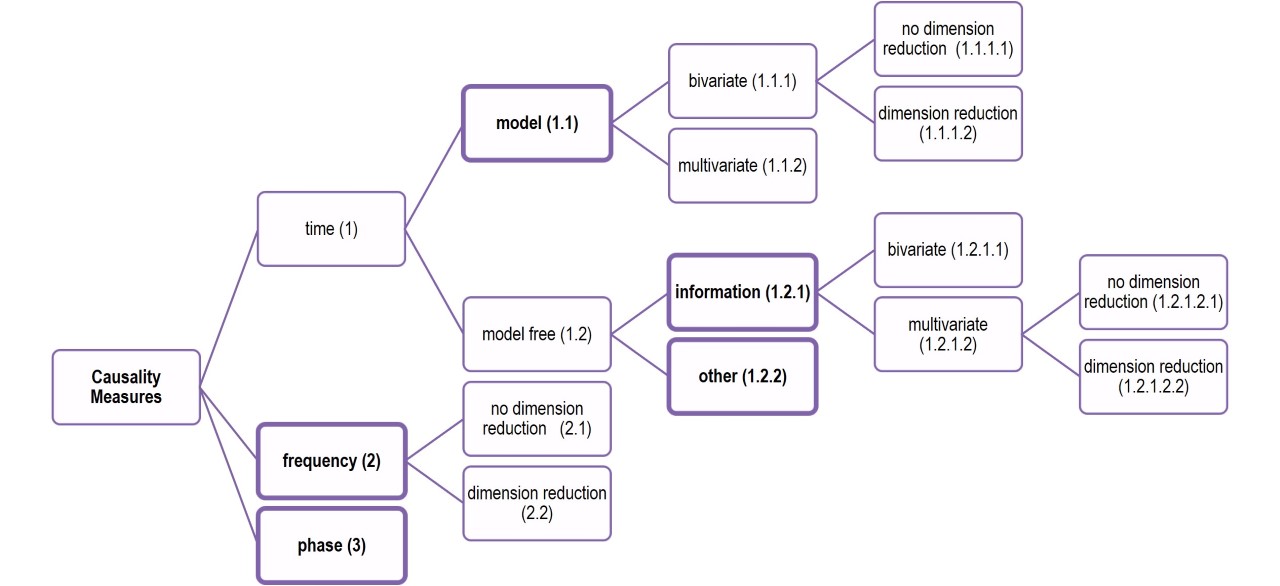
Figure 1: Tree structure for the types of causality measures. The five main classes are highlighted (frame box in bold). Each measure type in a box is given a code number, used as reference in Table LABEL:tab:MeasureList.

The measures in time domain dominate and they are further divided in model-based and model-free measures. Many of the model-free measures are based on information theory measures and the other model-free measures on the time domain are referred to as “other” measures. Thus five main classes of causality measures are considered in this study: model-based measures, information measures, frequency measures, phase measures and other measures that cannot be defined in terms of the other four classes. The measures organized in these five classes and included in the comparative study are briefly discussed below, and they are listed in Table LABEL:tab:MeasureList, with reference and code number denoting the type of measure (the class, bivariate or multivariate and with our without dimension reduction).

Table 1: List of causality measures organized in the five classes. The first column has the measure notation including the measure parameters, the second column has a brief description, the third column has the code of each measure denoting its type, and the fourth column has a related reference.

Symbol	Description	Type	Ref.
Model-based
GCI($p$)	Granger causality index, $p$ is the VAR order, for Hénon maps $p\!=\!2,5$, for VAR process $p\!=\!3,5$, for Mackey-Glass system and neural mass model $p\!=\!5,10,20$	1.1.1.1	Granger (1969)
CGCI($p$)	Conditional Granger causality index	1.1.2	Geweke (1984)
PGCI($p$)	Partial Granger causality index	1.1.2	Guo et al. (2008)
RCGCI($p$)	Restricted Granger causality index	1.1.1.2	Siggiridou and Kugiumtzis (2016)
Information
TE($m,\tau$)	Transfer entropy. Lag $\tau\!=\!1$ for all systems, embedding dimension for Hénon maps $m\!=\!2,3$, for VAR process $m\!=\!3,5$, for Mackey-Glass system and neural mass model $m\!=\!5,10,15$	1.2.1.1	Schreiber (2000)
PTE($m,\tau$)	Partial transfer entropy	1.2.1.2.1	Papana et al. (2012)
STE($m,\tau$)	Symbolic transfer entropy	1.2.1.1	Staniek and Lehnertz (2008)
PSTE($m,\tau$)	Partial symbolic transfer entropy	1.2.1.2.1	Papana et al. (2015)
TERV($m,\tau$)	Transfer entropy on rank vectors	1.2.1.1	Kugiumtzis (2012)
PTERV($m,\tau$)	Partial transfer entropy on rank vectors	1.2.1.2.1	Kugiumtzis (2013)
PMIME($L$)	Partial mutual information from mixed embedding, maximum lag for Hénon maps and VAR model $L_{max}\!=\!5$, for Mackey-Glass system and neural mass model $L_{max}\!=\!20$	1.2.1.2.2	Kugiumtzis (2013)
Frequency
PDC($p,i$)	Partial directed coherence, $i$ denotes the power band $i\!=\!\delta,\theta,\alpha,\beta,\gamma$ (relative proportion of the whole spectrum). For Hénon maps $p\!=\!2,5$, for the VAR process $p\!=\!3,5$, for the Mackey-Glass system and the neural mass model $p\!=\!5,10,20$	2.1	Baccalá and Sameshima (2001)
GPDC($p,i$)	Generalized partial directed coherence	2.1	Baccala et al. (2007)
DTF($p,i$)	Directed transfer function	2.1	Kaminski and Blinowska (1991)
dDTF($p,i$)	Direct directed transfer function	2.1	Korzeniewska et al. (2003)
GGC($p,i$)	Geweke’s spectral Granger causality	1.1.1.1	Hu et al. (2011)
RGPDC($p,i$)	Restricted generalized partial directed coherence	2.2	Siggiridou et al. (2017)
Phase
DPI	Phase directionality index	3	Rosenblum and Pikovski (2001)
Other
MCR($m,\tau$)	Mean conditional recurrence, $m$ is the same as for the information measures	1.2.2	Romano et al. (2007)
DED	Directed event delay	1.2.2	Quian Quiroga et al. (2002)

The first class of model-based measures regards measures that implement the original concept of Granger causality, the bivariate measure of Granger causality index (GCI) Granger (1969) (only $X$ and $Y$ variables are considered), and the multivariate measures of the conditional Granger causality index (CGCI) Geweke (1984) and the partial Granger causality (PGCI) Guo et al. (2008) (also the other observed variables denoted $Z$ are included). All these measures require the fit of a vector autoregressive model (VAR), on the two or more variables. The order $p$ of VAR denoting the lagged variables of each variable contained in the model can be estimated by an information criterion such as AIC or BIC, which often does not provide optimal lags, e.g. see the simulation study in Hatemi-J and Hacker (2012) and citations therein, and the so-called $p$-hacking (in the sense of $p$-value) in terms of VAR models for Granger causality in Bruns and Stern (2019). To overcome the use of order estimation criteria, here we use a couple of predefined appropriate orders $p$ for each system (see Table LABEL:tab:MeasureList). In the presence of many observed variables, dimension reduction in VAR has been proposed, and here we use the one developed from our team, the restricted conditional Granger causality index (RCGCI) Siggiridou and Kugiumtzis (2016). Thus for this class of measures, there are bivariate and multivariate measures, and multivariate measures that apply dimension reduction, as noted in the sketched division of causality measures in Fig.1. These are all linear measures and besides this constraint they have been widely used in applications. Other nonlinear extensions are not considered in this study for two reasons: either they were very computationally intensive, such as the cross predictions of local state space models Faes et al. (2008), or they were too complicated so that discrepancies to the original methods may occur Montalto et al. (2015); Abbasvandi and Nasrabadi (2019).

The information measures of the second class have also been popular in diverse applications recently due to their general form, as they do not require any specific model, they are inherently nonlinear measures and can be applied to both deterministic systems and stochastic processes of any type, e.g. oscillating flows and discrete maps of any dimension. The main measure they rely on is the mutual information (MI), and more precisely the conditional mutual information (CMI). There have been several forms for causality measures based on MI and CMI in the literature, e.g. see the coarse-grained mutual information in Paluš et al. (2001), but the prevailing one is the transfer entropy (TE), originally defined for two variables Schreiber (2000). The multivariate version, termed partial transfer entropy (PTE) was later proposed together with different estimates of the entropies involved in the definition of PTE, bins Verdes (2005), correlation sums Vakorin et al. (2009) and nearest neighbors Papana et al. (2012). Here, we consider the nearest neighbor estimate for both TE and PTE, found to be the most appropriate for high dimensions. Equivalent forms to TE and PTE are defined for the ranks of the embedding vectors rather than the observations directly. We consider the bivariate measures of symbolic transfer entropy (STE) Staniek and Lehnertz (2008) and transfer entropy on rank vectors (TERV) Kugiumtzis (2012), and the multivariate measures of partial symbolic transfer entropy (PSTE) Papana et al. (2015) and partial transfer entropy on rank vectors (PTERV) Kugiumtzis (2013). The idea of dimension reduction was implemented in TE first, applying a scheme for a sparse non-uniform embedding of both $X$ and $Y$, termed mutual information on mixed embedding (MIME) Vlachos and Kugiumtzis (2010). This bivariate measure was later extended to the multivariate measure of partial MIME (PMIME) Kugiumtzis (2013). Only the PMIME is included in the study simply due to the computational cost, and it is noted that by construction the measure gives zero for insignificant causal effects, so it does not require binarization when networks of binary connections have to be derived (the positive values are simply set to one).

All the methods in the third class of frequency measures rely on the estimation of the VAR model, either on only the two variables $X$ and $Y$ or on all the observed variables (we consider only the latter case here). Geweke’s spectral Granger causality (GGC) is the early measure implementing the concept of Grangre causality in the frequency domain Geweke (1982); Hu et al. (2011), included in the study. Another older such measure included in the study is the direct transfer function (DTF) Kaminski and Blinowska (1991), which although it is multivariate measure it does not discriminate direct from indirect causal effects. For this, an improvement is proposed and used also in this study, termed direct directed transfer function (dDTF) Korzeniewska et al. (2003). We also consider the partial directed coherence (PDC) Baccalá and Sameshima (2001) and the improved version of generalized partial directed coherence (GPDC) Baccala et al. (2007), which have been particularly popular in EEG analysis. When applied to EEG, the measures are defined in terms of frequency bands of physiological relevance ($\delta$, $\theta$, $\alpha$, $\beta$, $\gamma$, going from low to high frequencies), and the same proportional split of the frequency range is followed here (as if the sampling frequency was 100 Hz). Finally, we consider a dimension reduction of VAR in the GPDC measure called restricted GPDC (RGPDC), recently proposed from our team Siggiridou et al. (2017).

As mentioned above the class of phase measures contains a good number of measures used in connectivity analysis, mainly in neuroscience dealing with oscillating signals such as EEG, but most of these measures are symmetric and thus out of the scope of the current study. In the evaluation of the causality measures we consider the bivariate measure of phase directionality index (DPI) Rosenblum and Pikovski (2001), which is a measure of synchronization designed for oscillating time series. Information measures have also been implemented in the phases, e.g. see Paluš and Stefanovska (2003), but not considered here.

Another class of measures used mainly in neuroscience regards inter-dependence measures based on neighborhoods in the reconstructed state space of each of the two variables $X$ and $Y$. A series of such measures have been proposed after the first work in Arnhold et al. (1999), using also ranks of the reconstructed vectors Chicharro and Andrzejak (2009), the latter making the measure computationally very slow. The convergent cross mapping is developed under the same approach Sugihara et al. (2012), and the same yields for the measure of mean conditional recurrence (MCR) Romano et al. (2007). It is noted that all these measures are bivariate and they are expected to suffer from estimating indirect connections in the estimated causality network. The MCR is included as a representative of the state space bivariate measures in the class of other measures. In this class, we include also event synchronization measures Quian Quiroga et al. (2002), and specifically the direct event delay (DED) that is a directional bivariate measure, considered as causality measure and included in the study.

For the information measures where the estimation of entropies in high dimensions is hard, the comparison of the multivariate measures that do not include dimension reduction to these including dimension reduction would be unfair when high-dimensional systems are considered. To address this, in the calculation of a multivariate information measure not making use of dimension reduction, we choose to restrict the set of the conditioning variables $Z$ in the estimated causal effect $X\rightarrow Y|Z$ to only the three more relevant variables. In the simulations, we consider the number of observed variables (equal to the subsystems being coupled) to be $K\!=\!5$ and $K\!=\!25$. While for $K\!=\!5$ all the remaining variables are considered in $Z$, for $K\!=\!25$ only three of the remaining 23 variables are selected. The criterion of selection is the mutual information of the remaining variables to the driving variable $X$, which is common for the selection of variables Marinazzo et al. (2012).

2.2 Identification of original network connections

We suppose that a dynamical system is formed by the coupling of $K$ subsystems and we observe one variable from each subsystem, so that a multivariate time series of dimension $K$ is derived. The coupling structure of the original system can be displayed as a network of $K$ nodes where the connections are determined by the system equations. Formally, in the graph-theoretical framework, a network is represented by a graph $G\!=\!(V;E)$, where $V$ is the set of $K$ nodes, and $E$ is the set of the connections among the nodes of $V$. The original coupling network is given as a graph of directed binary connections, where the connection from node $i$ to node $j$ is assigned with a value $a_{i,j}$ being one or zero, depending whether variables of the subsystem $i$ are present in the equation determining the variables of the subsystem $j$. The components $a_{i,j}$, $i,j\!=\!1,\ldots,K$, form the adjacency matrix $A$ that defines the network.

The computation of any causality measure presented in Sec. 2.1 on all the directed pairs $(i,j)$ of the $K$ observed variables gives a weight matrix $R$ (assuming only positive values of the measure, so that a transformation of the measure can be applied if necessary). Thus, the pairwise causality matrix $R$ with entries $R_{i,j}\!=\!R_{X_{i}\rightarrow X_{j}}$ defines a network of weighted connections, assigning the weighted directed connection $R_{i,j}$ from each node $i$ to each node $j$.

In applications, often binary networks are sought to better represent the estimated structure of the underlying system. Here, we are interested to compare how the causality measure retrieves the original directed coupling structure, and therefore we want to transform the weighted network to a binary network. Commonly, the weighted matrix $R$ is transformed into an adjacency matrix $A$ by suitable thresholding, keeping in the graph only connections with weights higher than some threshold (and setting their weights to one) and removing the weaker connections (setting their weights to zero). For each causality measure, an appropriate threshold criterion is sought to determine the significant values of the measure that correspond to connections in the binary network. We consider three approaches for thresholding that have been used in the literature.

1. Rigorous thresholding is provided by appropriate significance test for the causality measure $R_{X_{i}\rightarrow X_{j}}$. For all considered causality measures in this study, we expect the causality measure to lie at the zero level if there is no causal effect and be positive if it is, so that the test is one-sided. So, the null and alternative hypotheses are respectively:

   $$\mbox{H}_{0}:R_{X_{i}\rightarrow X_{j}}=0,\quad\quad\mbox{H}_{1}:R_{X_{i}\rightarrow X_{j}}>0$$ (1)

   Parametric significance tests have been developed only for the linear causality measures, and for consistency we apply the randomization significance test to all causality measures, making use of the simple technique of time-shifted surrogates. Specifically, we generate $M$ resampled (surrogates) time series for the driving variable $X$, each by shifting cyclically the original observations of $X$ by a random step $w$. For the original time series of the driving variable $X_{i}$ denoted $\{X_{i,t}\}\!=\!\{x_{1,t},x_{2,t},\ldots,x_{n,t}\}$, the surrogate time series is $\{X_{i,t}^{*}\}\!=\!\{x_{w+1,t},x_{w+2,t},\ldots,x_{n,t},x_{1,t},\ldots,x_{w-1,t},x_{w,t}\}$. In this way we destroy any form of coupling of $X_{i}$ and any other variable $X_{j}$, so that $\{X_{i,t}^{*}\}$ is consistent to $H_{0}$, but it preserves the dynamics and the marginal distribution of $X_{i}$. The test statistic is the causality measure $R_{X_{i}\rightarrow X_{j}}$, and it takes the value $R_{0}$ on the original time series pair and the values $R_{1},R_{2},\ldots,R_{M}$ on each of the $M$ resampled time series pairs. The rank of $R_{0}$ in the ordered list of $M+1$ values $R_{0},R_{1},R_{2},\ldots,R_{M}$, denoted $r_{0}$, defines the $p$-value of the randomization test as $p\!=\!1-\frac{r_{0}-0.326}{M+1+0.348}$ Yu and Huang (2001). If $R_{0}$ is at the right tail of the empirical distribution formed by $R_{1},R_{2},\ldots,R_{M}$, then the H₀ is rejected, which suggests that $p<\alpha$, where $\alpha$ is the significance level of the test determining the tail. For a multivariate time series of $K$ variables, totally $K(K-1)$ significance tests are performed for each causality measure, indicating that multiple tests are performed on the same dataset. This is a known issue in statistics and corrections for multiple testing can be further be applied, such as the false discovery rate Benjamini and Hochberg (1995). Here, we refrain from using such a correction and rather use three different significance levels $\alpha\!=\!0.01,0.05,0.1$. We opted for this as the same setting is applied for all causality measures.

2. The second thresholding criterion is given by the desired density of the binary network. In the simulation study, we know the density of the original network, denoted by the number of connections $\rho_{0}$. We consider five different values for the density $\rho$ of the estimated causality binary network given in multiples of $\rho_{0}$ as $0.6,0.8,1.0,1.2,1.4$.

3. The third thresholding criterion is simply given by a predefined magnitude threshold on the causality measure. Here, we select an appropriate threshold $th_{\rho}$ separately for each causality measure and each coupling strength for the same system, where $\rho$ indicates the corresponding density. Having 10 realizations for each scenario (system and coupling strength), the $th_{\rho}$ is the average of the thresholds found for the given density $\rho$ in the 10 realizations.

2.3 Performance indices for statistical evaluation of methods accuracy

For a system of $K$ variables there are $K(K-1)$ ordered pairs of variables to estimate causality. In the simulations of known systems, we know the true coupling pairs and thus we can compute performance indices to rate the causality measures as for their overall matching of the original connections in the network. Here, we consider the performance indices of specificity, sensitivity, Matthews correlation coefficient, F-measure and Hamming distance.

The sensitivity is the proportion of the true causal effects (true positives, TP) correctly identified as such, given as sens=TP/(TP+FN), where FN (false negatives) denotes the number of pairs having true causal effects but have gone undetected. The specificity is the proportion of the pairs correctly not identified as having causal effects (true negatives, TN), given as spec=TN/(TN+FP), where FP (false positives) denotes the number of pairs found falsely to have causal effects. An ideal causality measure would give values of sensitivity and specificity at one. To weigh sensitivity and specificity collectively we consider the Matthews correlation coefficient (MCC) Matthews (1975) given as

$$\text{MCC}=\frac{\text{TP}\cdot\text{TN}-\text{FP}\cdot\text{FN}}{\sqrt{(\text{TP}+\text{FP})\cdot(\text{TP}+\text{FN})\cdot(\text{TN}+\text{FP})\cdot(\text{TN}+\text{FN})}}.$$ (2)

MCC ranges from -1 to 1. If MCC=1 there is perfect identification of the pairs of true and no causality, if MCC=-1 there is total disagreement and pairs of no causality are identified as pairs of causality and vice versa, whereas MCC at the zero level indicates random assignment of pairs to causal and non-causal effects.

Similarly, we consider the F-measure that combines precision and sensitivity. The precision, called also positive predictive value, is the number of detected true causal effects divided by the total number of detected casual effects, given as prec=TP/(TP+FP), and the F-measure (FM) is defined as

$$\mbox{FM}=\frac{2\cdot\text{prec}\cdot\text{sens}}{\text{prec}+\text{sens}}=\frac{2\text{TP}}{2\text{TP}+\text{FN}+\text{FP}},$$

which ranges from 0 to 1. If FM=1 there is perfect identification of the pairs of true causality, whereas if FM=0 no true coupling is detected.

The Hamming distance (HD) is the sum of false positives (FP) and false negatives (FN), HD=FP+FN. Thus HD gets non-negative integer values bounded below by zero (perfect identification) and above by $K(K-1)$ if all pairs are misclassified.

2.4 Score Index

In Sec. 2.3, we presented five performance indices to evaluate in different ways the match of the original network and the estimated network from each causality measure. Further, we want to quantify this match for different settings, which involve different systems and different scenarios for each system regarding the number of variables $K$, the system free parameter, the time series length $n$ and the coupling strength $C$, where applicable (to be presented below in Sec. 2.5). For this, we rely on the index MCC, and for each scenario of a different system, we rank the causality measures according to their average MCC (across 10 realizations generated per scenario). For equal MCC, ordinal ranking (called also $"1234"$ ranking) is adopted Lansdown (1998). Specifically, the order of measures of equal MCC is decided from distinct ordinal numbers given at random to each measure of equal MCC value. Next, we derive the average rank of a causality measure $i$ for all different coupling strengths $C$ of a system $j$, $P_{i,j}$, as the average of the ranks of the causality measure $i$ in all coupling strengths tested for the system $j$. A score $s_{i,j}$ of the causality measure $i$ for the system $j$ is then derived by normalization of the average rank $P_{i,j}$ over the number $N$ of all measures so as to scale between zero and one, $s_{i,j}\!=\!(N-P_{i,j})/(N-1)$, where one is for the best measure ranked at top. The overall score of the causality measure $i$ over all systems, $s_{i}$, is simply given by the average $s_{i,j}$ over all systems, including the two different $K$ values for systems S1, S2 and S3, the two values for the system parameter $\Delta$ and $A$ for systems S2 and S3, respectively, and the two time series lengths $n$ for system S1. The systems are presented in the next section.

2.5 Synthetic systems

For the comparative study, we use four systems with different properties: the coupled Hénon maps as an example of discrete-time chaotic coupled system Kugiumtzis (2013), the coupled Mackey-Glass system as an example of continuous-time chaotic coupled system but of high complexity Senthilkumar et al. (2008); Kugiumtzis (2013), the so-called neural mass model as an example of a continuous-time stochastic system used as an EEG model Wendling et al. (2000); Koutlis and Kugiumtzis (2016), and the vector autoregressive model (VAR) as suggested in Basu and Michailidis (2015), used as an example of a discrete-time linear stochastic process. The four systems are briefly presented below.

S1: The system of coupled Hénon maps is a system of coupled chaotic maps defined as

$$\begin{array}[]{ll}x_{i,t}=1.4-x_{i,t-1}^{2}+0.3x_{i,t-2},&\mbox{for}\,\,i=1,K\\ x_{i,t}=1.4-\left(0.5C(x_{i-1,t-1}+x_{i+1,t-1})+(1-C)x_{i,t-1}\right)^{2}+0.3x_{i,t-2},&\mbox{for}\,\,j=2,\ldots,K-1\end{array}$$ (3)

where $K$ denotes the number of variables and $C$ is the coupling strength. We consider the system for $K\!=\!5$ and $K\!=\!25$ and the corresponding coupling network is shown in Fig. 2a and b, respectively.

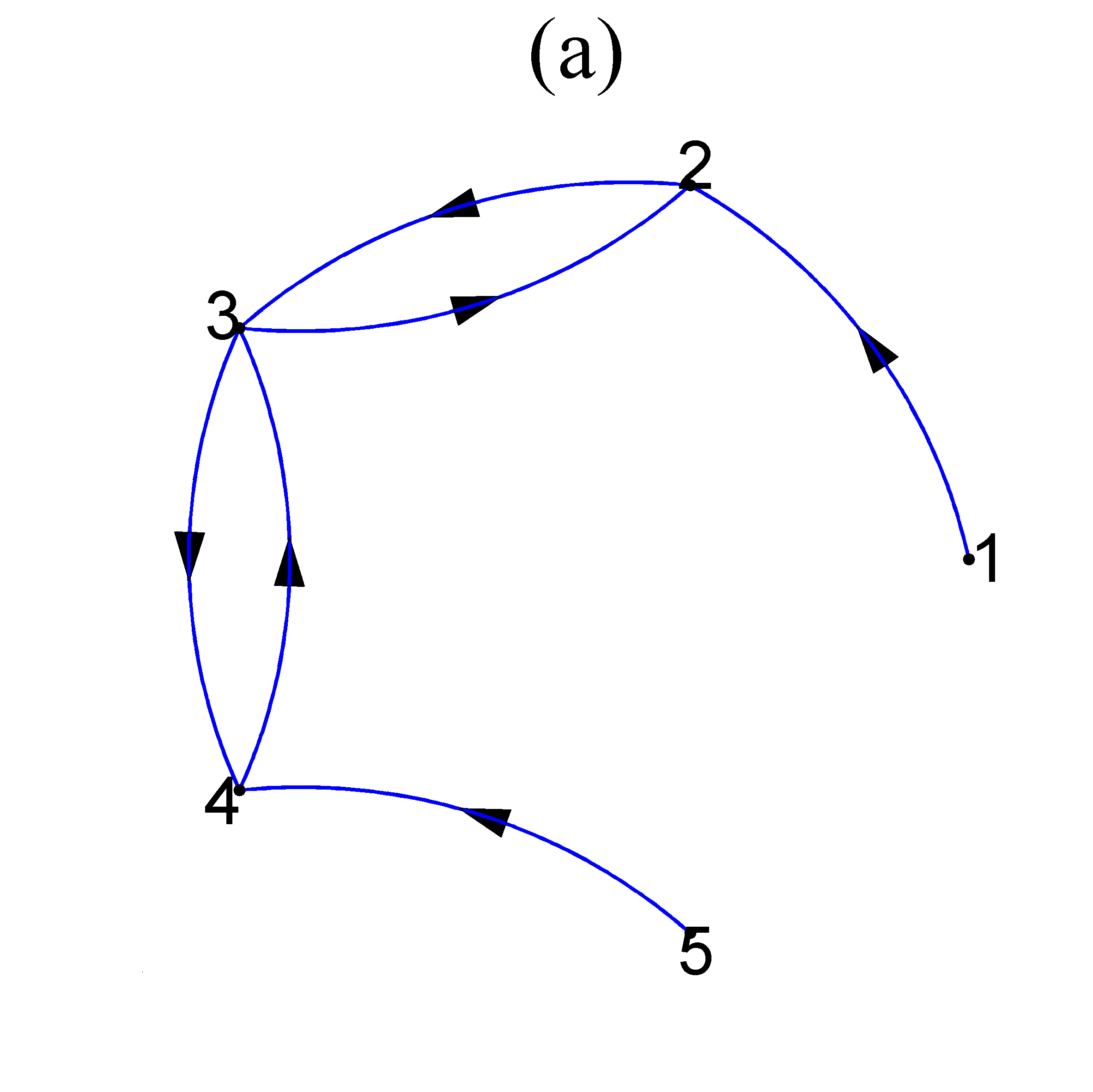
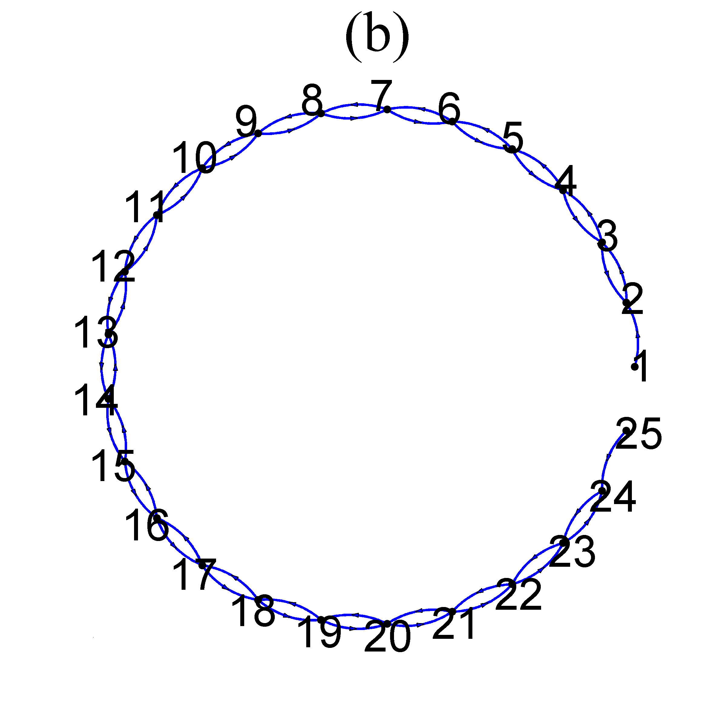
Figure 2: Coupling networks for S1, S2, S3 in (a) for $K\!=\!5$, in (b) for $K\!=\!25$ , and in (c) for S4 and $K\!=\!25$.

Multivariate time series of size $K$ are generated and we use short and long time series of length $n\!=\!512$ and $n\!=\!2048$, respectively. An exemplary time series for $K\!=\!5$ is given in Fig. 3a.

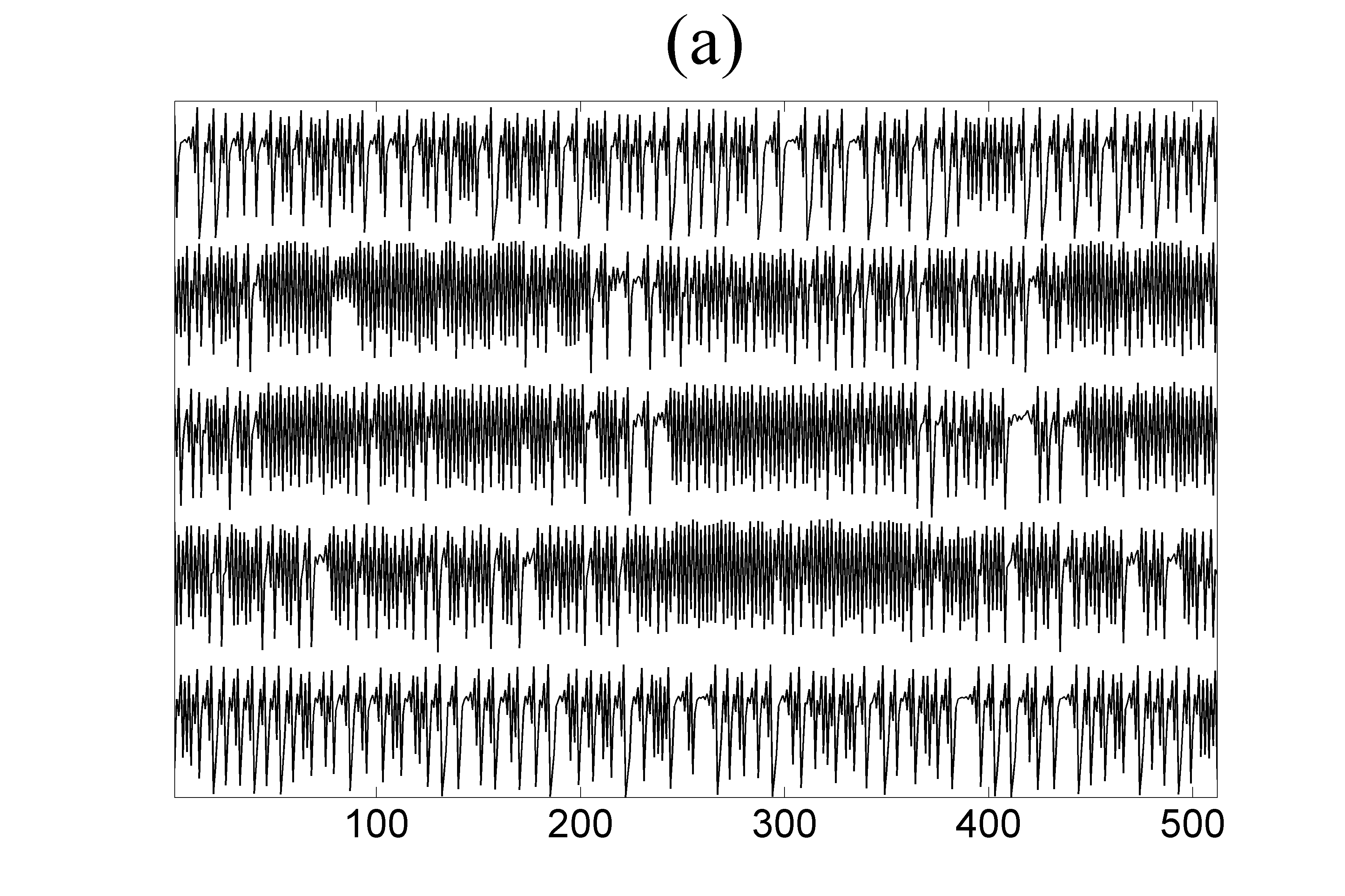
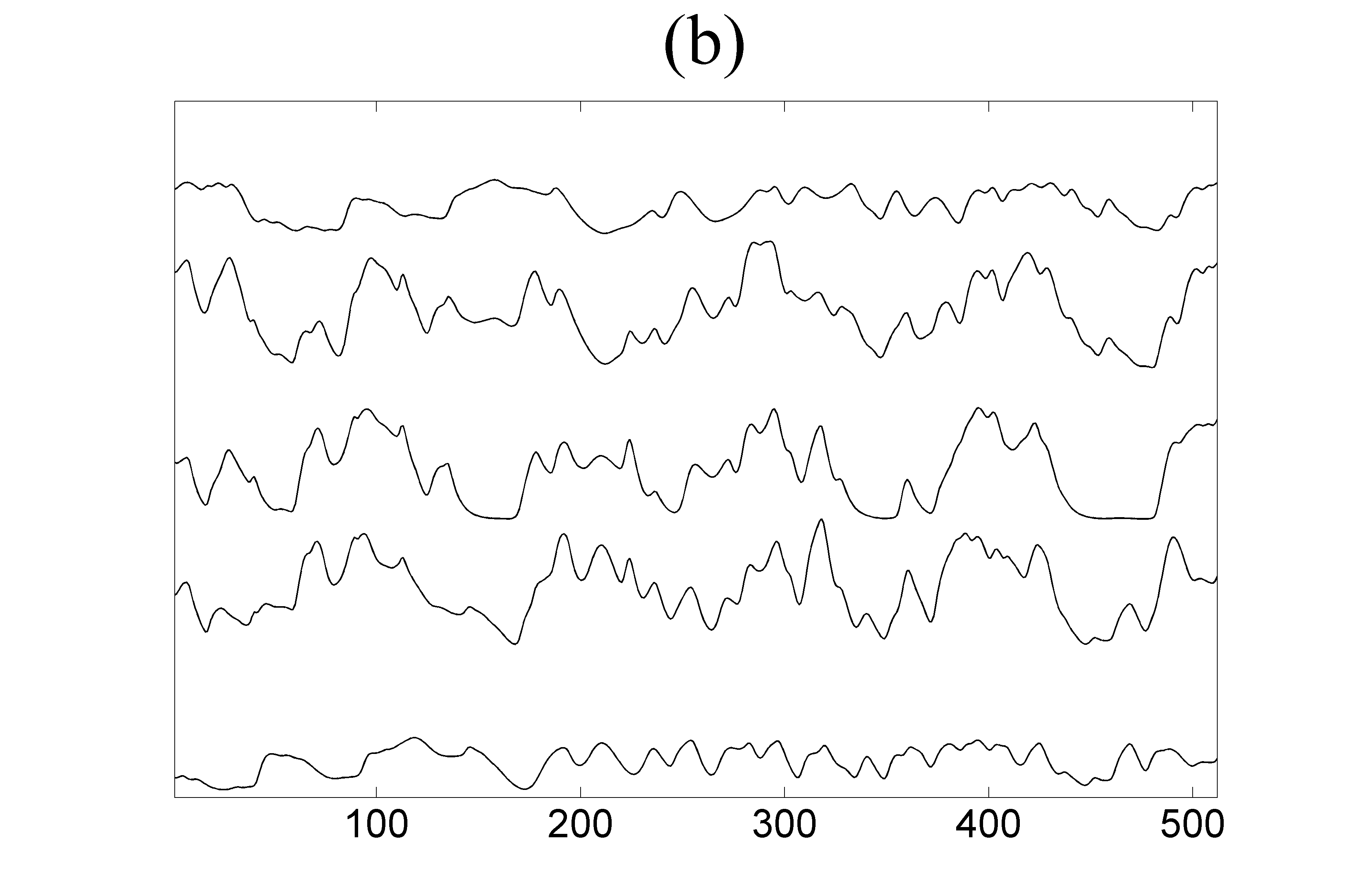
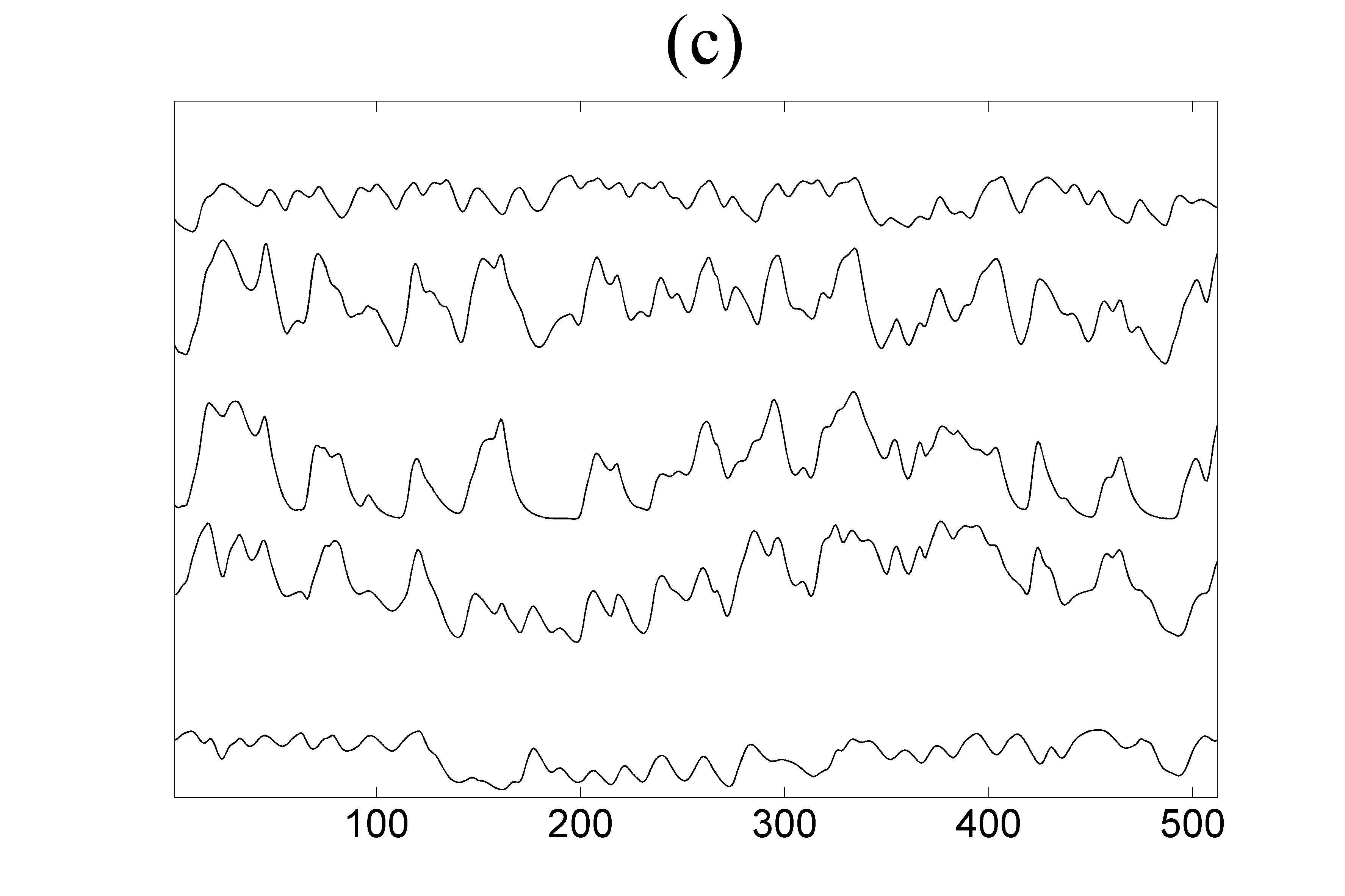
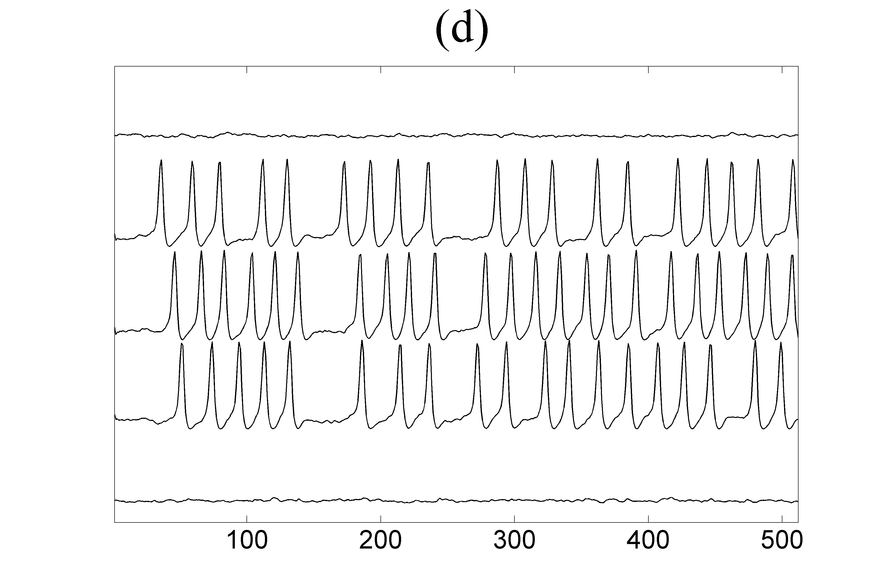
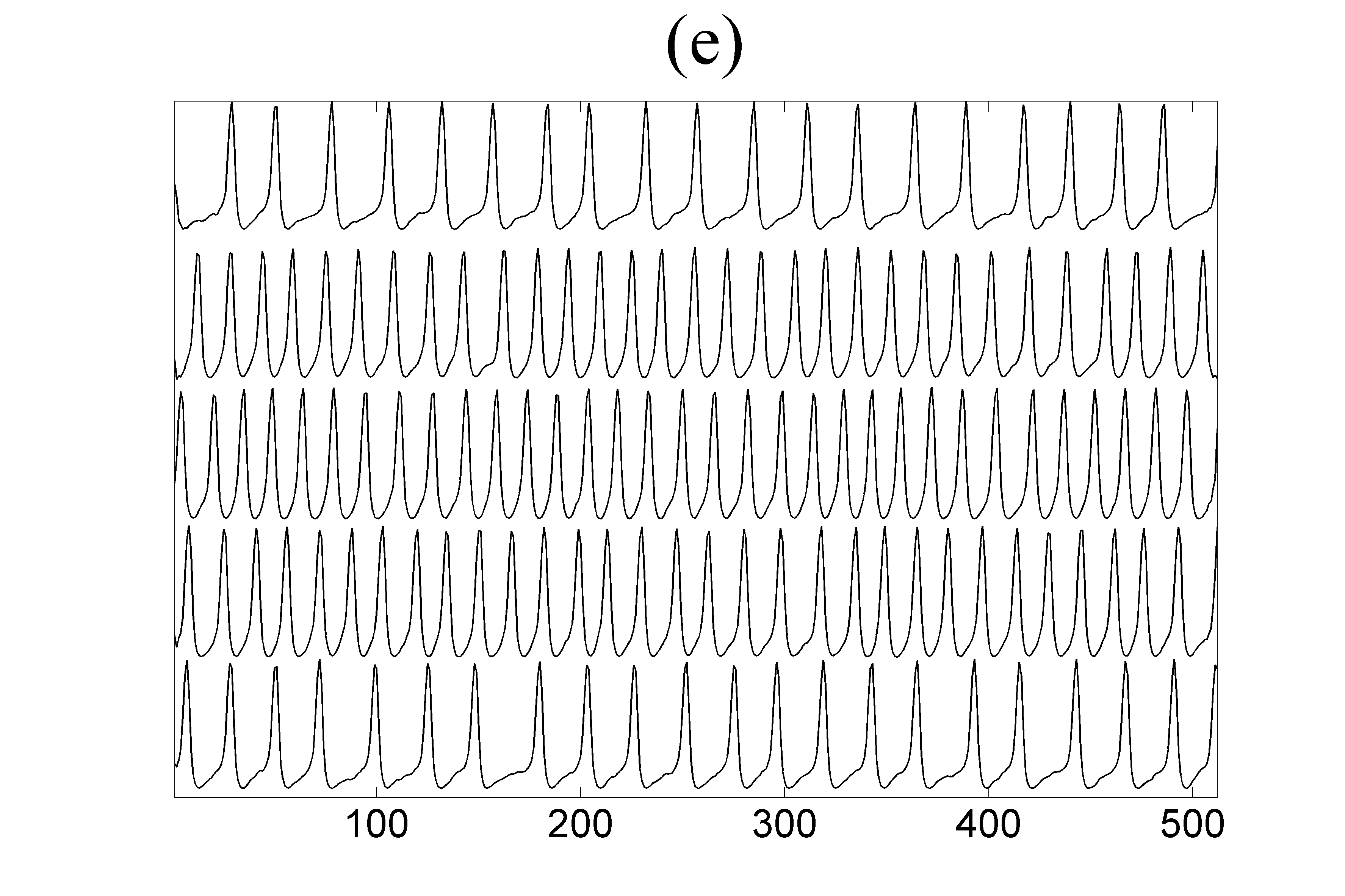
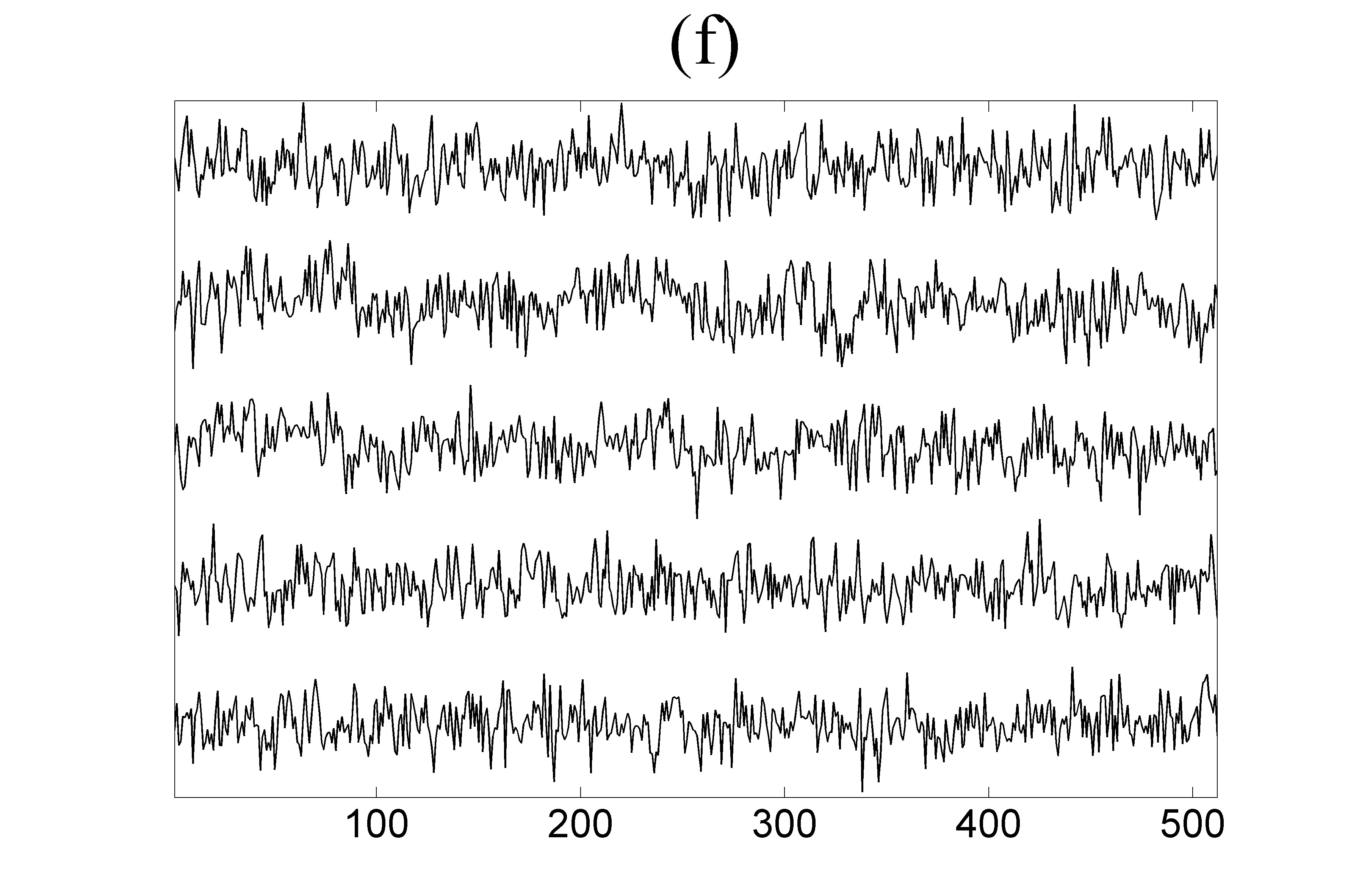
Figure 3: Time series for: (a) coupled Hénon maps for $C\!=\!0.2$, (b) coupled Mackey-Glass for $\Delta\!=\!100$ and $C\!=\!0.2$, (c) coupled Mackey-Glass for $\Delta\!=\!300$ and $C\!=\!0.2$, (d) neural mass for $A\!=\!3.45$ and $C\!=\!80$, (e) neural mass for $A\!=\!3.7$ and $C\!=\!80$, (f) VAR(3) model for $C\!=\!0.23$.

S2: The system of coupled Mackey-Glass is a system of coupled identical delayed differential equations defined as

$$\dot{x}_{j}(t)=-0.1x_{j}(t)+\sum_{i=1}^{K}\frac{C_{ij}x_{i}(t-\Delta)}{1+x_{i}(t-\Delta)^{10}}\quad\quad\mbox{for}\,\,j=1,2,\ldots,K$$ (4)

where $K$ is the number of subsystems coupled to each other, $C_{ij}$ is the coupling strength and $\Delta$ is the lag parameter. We set $C_{ii}\!=\!0.2$ and $C_{i,j}$ for $i\neq j$ zero or $C$ according to the ring coupling structure shown in Fig. 2a and b for $K\!=\!5$ and $K\!=\!25$, respectively. For details on the solution of the delay differential equations and the generation of the time series, see Kugiumtzis (2013). Two scenarios are considered regarding the inherent complexity of each of the $K$ subsystems given by $\Delta\!=\!100$ and $\Delta\!=\!300$, regarding high complexity (correlation dimension is about 7.0 Kugiumtzis (1996)) and even higher complexity (not aware of any specific study for this regime), respectively. Exemplary time series for each $\Delta$ and $K\!=\!5$ are given in Fig. 3b and c. The time series used in the study have length $n\!=\!4096$.

S3: The neural mass model is a system of coupled differential equations with a stochastic term that produces time series similar to EEG simulating different states of brain activity, e.g. normal and epileptic. It is defined as

$$\dot{y}_{0}^{j}(t)= y_{3}^{j}(t)$$ (5)

$$\dot{y}_{3}^{j}(t)= AaS[y_{1}^{j}(t)-y_{2}^{j}(t)]-2ay_{3}^{j}(t)-a^{2}y_{0}^{j}(t)$$

$$\dot{y}_{1}^{j}(t)= y_{4}^{j}(t)$$

$$\dot{y}_{4}^{j}(t)= Aa\left\{p^{j}(t)+C_{2}S(C_{1}y_{0}^{j})+\sum_{\begin{subarray}{c}i=1\\ i\neq j\end{subarray}}^{K}C_{ij}y_{6}^{i}(t)\right\}$$

$$-2ay_{4}^{j}(t)-a^{2}y_{1}^{j}(t)$$

$$\dot{y}_{2}^{j}(t)= y_{5}^{j}(t)$$

$$\dot{y}_{5}^{j}(t)= Bb\left\{C_{4}S[C_{3}y_{0}^{j}(t)]\right\}-2by_{5}^{j}(t)-b^{2}y_{2}^{j}(t)$$

$$\dot{y}_{6}^{j}(t)= y_{7}^{j}(t)$$

$$\dot{y}_{7}^{j}(t)= Aa_{d}S(y_{1}^{j}(t)-y_{2}^{j}(t))-2a_{d}y_{7}^{j}(t)-a_{d}^{2}y_{6}^{j}(t)$$

where $j$ denotes each of the $K$ subsystems representing the neuron population defined by eight interacting variables and the population (subsystem) interacts with other populations through variable $y_{4}^{j}$ with coupling strength $C_{ij}$. We set $C_{ii}\!=\!0.0$ and $C_{i,j}$ for $i\neq j$ zero or $C$ according to the ring coupling structure shown in Fig. 2a and b for $K\!=\!5$ and $K\!=\!25$, respectively. The term $p^{j}(t)$ represents a random influence from neighboring or distant populations, $A$ is an excitation parameter and $B$, $a$, $b$, $a_{d}$, $C1$-$C4$ other parameters (see Wendling et al. (2000) for more details). The function $S$ is the sigmoid function $S(v)\!=\!2e_{0}/(1+e^{r(v_{0}-v)})$, where $r$ is the steepness of the sigmoid and $e_{0}$, $v_{0}$ are other parameters explained in Wendling et al. (2000). From each population $j=1,\ldots,K$ we consider only the first variable ${y}_{0}^{j}$ and obtain the multivariate time series of $K$ variables. The value of the excitation parameter $A$, affects the form of the output signals combined with the coupling strength level, ranging from similar to normal brain activity with no spikes to almost periodic with many spikes similar to epileptic brain activity. We consider two values for this parameter, one for low excitation with $A\!=\!3.45$ and one for high excitation with $A\!=\!3.7$. Exemplary time series for each $A$ and $K\!=\!5$ are given in Fig. 3d and e. The time series used in the study have length $n\!=\!4096$.

S4: The VAR process on $K\!=\!25$ variables and order $P\!=\!3$ as suggested in Basu and Michailidis (2015) is used as representative of a high-dimensional linear stochastic process. Initially, 4% of the coefficients (total coefficients 1875) of VAR(3) selected randomly are set to 0.9 and the rest are zero and the positive coefficients are reduced iteratively until the stationarity condition is fulfilled. The autoregressive terms of lag one are set to one. The true couplings are 8% of a total of 600 possible ordered couplings. An exemplary coupling network of random type is shown in Figure 2(c). The time series length is set to $n\!=\!512$ and an exemplary time series of only five of the $K\!=\!25$ variables of the VAR(3) process is shown in Fig. 3f.

For S1, S2 and S3, the coupling strength $C$, fixed for all couplings, is varied to study a wide range of coupling levels from zero coupling to very strong coupling. Specifically, for S1 and S2 $C\!=\!0,0.05,0.1,0.2,0.3,0.4,0.5$, and for S3 $C\!=\!0,20,40,80,120,160,200$. For S4, only one case of coupling strength is considered, given by the magnitude $0.23$ of all non-zero coefficients, for which the stationarity of VAR(3) process is reached. For each system and scenario of different coupling strength, 10 multivariate time series (realizations) are generated to obtain statistically valid results. The evaluation is performed as described in Section 2.4.

3 Results

In this section, the evaluation of the performance of all causality measures is presented for each system and scenario. First, the procedure of the evaluation is shown in one specific setting, then the measures are evaluated and ranked for each system and finally the overall ranking is given.

3.1 Evaluation of measures in one exemplary setting

We consider a multivariate time series of length $n\!=\!512$ from the system S1 of coupled Hénon maps for $K\!=\!5$ variables and coupling strength $C\!=\!0.2$. The original coupling network has the ring structure as shown in Fig. 2a. We derive the estimated causality (weight) matrix by the bivariate measure of transfer entropy (TE) using the appropriate parameters of embedding dimension $m\!=\!2$ and $\tau\!=\!1$

$$R_{\mbox{\scriptsize TE}}=\left(\begin{array}[]{ccccc}0&\textbf{0.148}&-0.003&-0.002&-0.012\\ -0.005&0&\textbf{0.167}&\textbf{0.013}&-0.021\\ -0.015&\textbf{0.094}&0&\textbf{0.051}&-0.004\\ -0.015&\textbf{0.016}&\textbf{0.092}&0&-0.014\\ -0.011&-0.009&0.003&\textbf{0.193}&0\\ \end{array}\right)$$ (6)

where the negative values denote the negative bias in the estimation of TE with the nearest neighbors estimate. Applying the three criteria of measure significance for transforming the weight matrix to an adjacency matrix (see Sec. 2.2), we derive the causality binary networks. Specifically, as shown in Fig. 4, different binary networks are obtained for the different values of the significance level of the randomization test, the network density and the magnitude threshold.

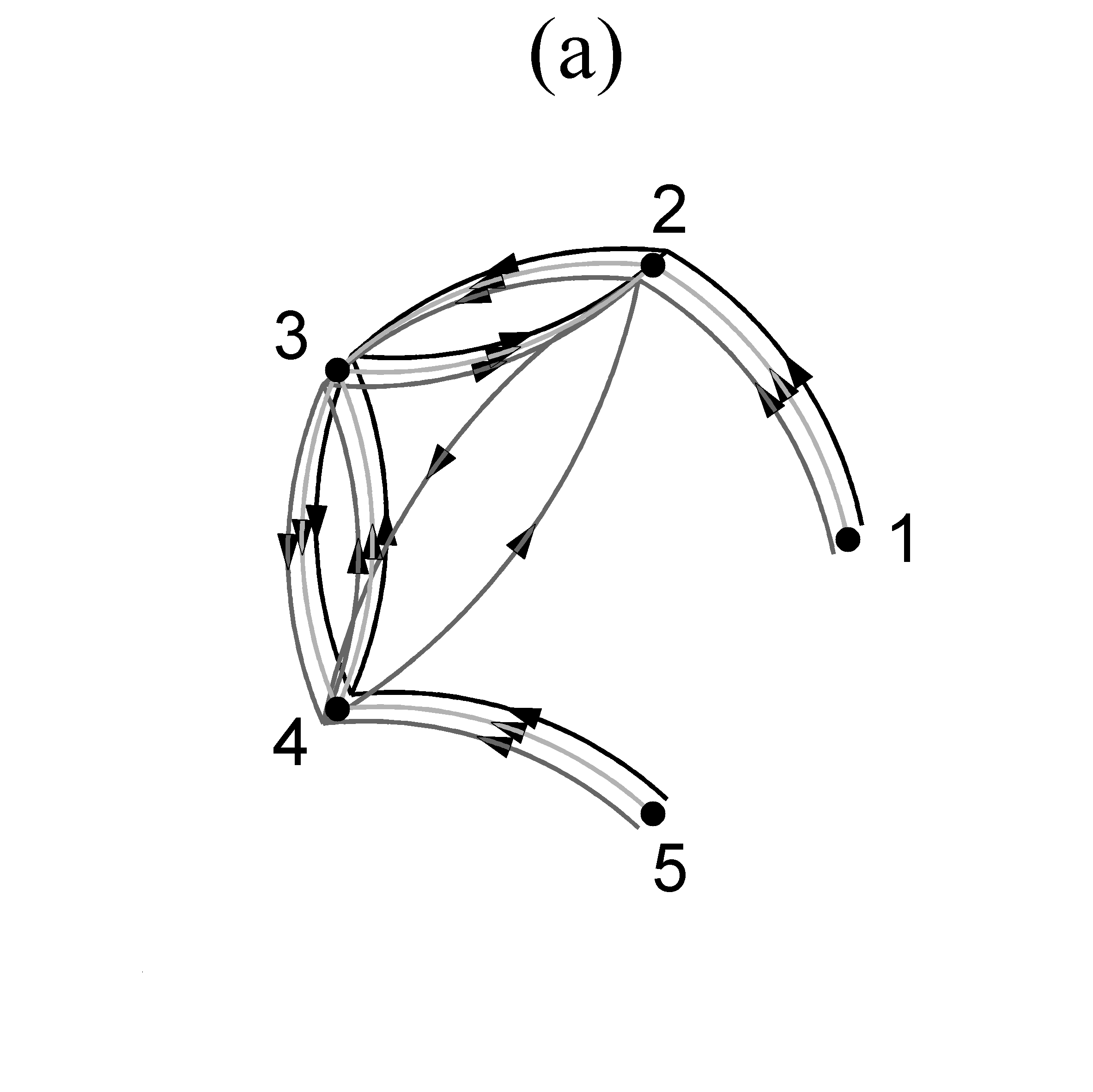
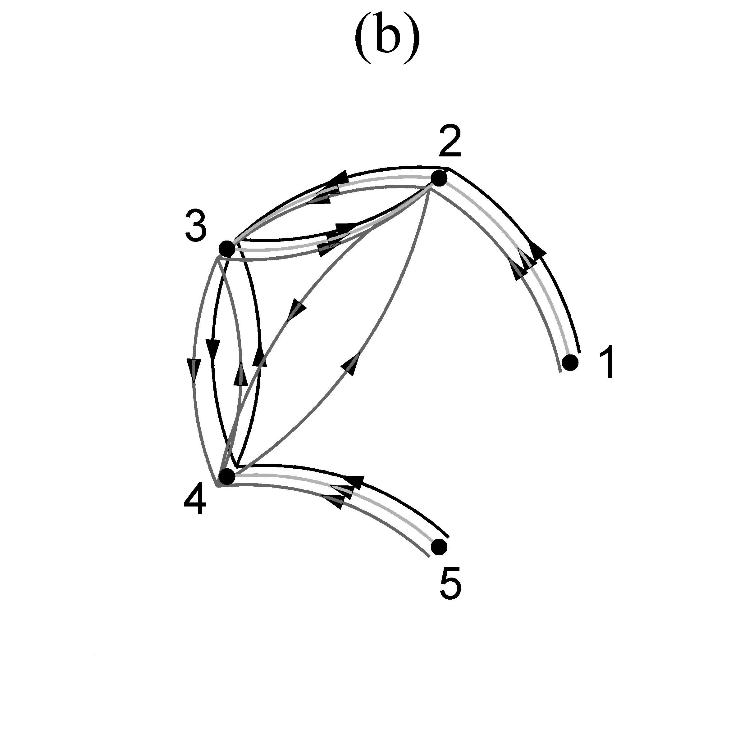
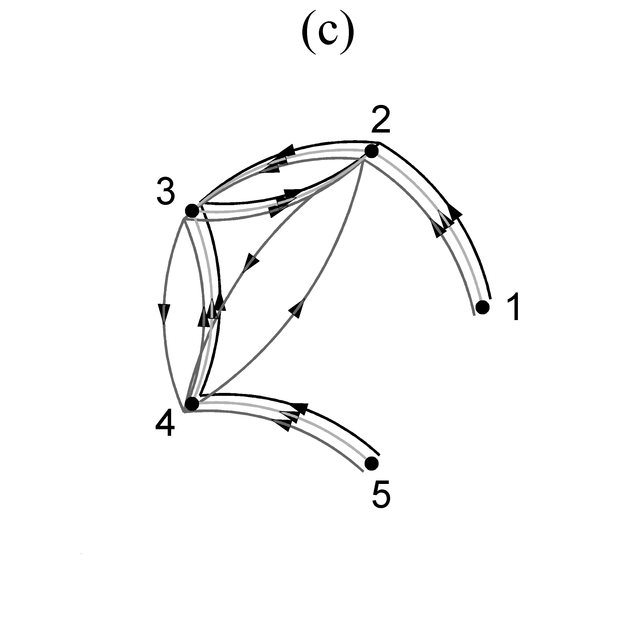
Figure 4: Binary networks of TE measure for S1 using (a) statistical significance test (light grey $\rightarrow$ $\alpha\!=\!0.01$ , black $\rightarrow$ $\alpha\!=\!0.05$, grey $\rightarrow$ $\alpha\!=\!0.1$), (b) density threshold (light grey $\rightarrow$ $\rho\!=\!4$ , black $\rightarrow$ $\rho\!=\!6$, grey $\rightarrow$ $\rho\!=\!8$) and (c) magnitude threshold (light grey $\rightarrow$ $th_{4}$ , black $\rightarrow$ $th_{6}$, grey $\rightarrow$ $th_{8}$)

In Fig. 4a, the binary network for significance level $\alpha\!=\!0.01$ and $\alpha\!=\!0.05$ coincides with the original coupling network, whereas for $\alpha\!=\!0.1$ more connections are present regarding indirect causal effects (for the latter the statistical significant values are given in bold in the form of eq.(6)). When preserving the 4, 6, and 8 strongest connections, as shown in Fig. 4b, the true structure is preserved only when the correct density is set (6 connections), indicating that the highest TE values are reached at the true couplings. This seems the optimal strategy for thresholding, but in real-world applications the actual network density is not a-priori known. Similarly, in Fig. 4c, the binary networks obtained using three magnitude thresholds on TE values are shown. Each of the three magnitude thresholds is computed as the average threshold for preserving the corresponding network density across 10 realizations, for this specific coupling strength and causality measure. These magnitude thresholds happen not to be the ones corresponding to the network densities for this realization and actually none of the three thresholds identifies all the existing and non-existing connections.

For illustration purposes, we compute the performance indices for TE at this scenario using the statistical significance criterion for $\alpha\!=\!0.1$, given in Table 2.

Table 2: Computation of the performance indices for the causality measure TE, where the binary causality network is derived using the statistical significance criterion for $\alpha\!=\!0.1$.

	true positive	true negative
positive found	$\mbox{TP}=6$	$\mbox{FP}=2$
negative found	$\mbox{FN}=0$	$\mbox{TN}=12$
sens : $6/6=1$
spec : $12/14=0.86$
MCC : $\frac{6\cdot 12-2\cdot 0}{\sqrt{(6+2)\cdot(6+0)\cdot(12+2)\cdot(12+0)}}$$=0.80$
FM : $\frac{2\cdot 6}{2\cdot 6+0+2}$$=0.86$
HD : $2+0=2$

We note that the two extra connections found significant using $\alpha\!=\!0.1$ reduce the specificity to 0.86 while sensitivity is one, which affects accordingly the other three measures. Note that the mismatch of just two out of 20 connections (HD=2) gives MCC=0.8, significantly lower from one, and the same holds for the F-measure index.

For the same scenario, the measure of PMIME (for a maximum lag $L\!=\!5$ well above the optimal lag 2) gives a weight matrix of zero and positive numbers

$$R_{\mbox{\scriptsize PMIME}}=\left(\begin{array}[]{ccccc}0&0.162&0&0&0\\ 0&0&0.101&0&0\\ 0&0.076&0&0.077&0\\ 0&0&0.094&0&0\\ 0&0&0&0.173&0\\ \end{array}\right)$$

No significance criterion is applied here, and simply setting the positive numbers to one gives the adjacency matrix, and in this case the estimated causality network matches exactly the original coupling network giving HD=0 and all other indices equal to one.

3.2 Results with respect to performance indices, significance criteria and coupling strength

First, we give a comprehensive presentation reporting all the performance indices presented in Sec. 2.3 and the significance criteria in Sec. 2.2 for system S1 and $K\!=\!25$, $n\!=\!2048$ and $C\!=\!0.2$. In Table 3, the five performance indices of the eight highest ranked causality measures in terms of MCC are presented.

Table 3: The rankings of the eight best measures according to MCC for coupled Hénon maps ($K\!=\!25$, $n\!=\!2048$, $C\!=\!0.2$) are presented for the three binarization methods. The sensitivity (sens), specificity (spec), F measure (FM) and Hamming distance (HD) performance indices are also presented.

	Measure	sens	spec	MCC	FM	HD
statistical significance test ($\alpha\!=\!0.05$)
1	PMIME($L\!=\!5$)	0.79	0.99	0.86	0.86	11
2	RGPDC($p\!=\!5$,$\beta$)	0.86	0.85	0.49	0.49	84.5
3	RGPDC($p\!=\!5$,$\alpha$)	0.87	0.84	0.47	0.47	91.6
4	GPDC($p\!=\!5$,$\beta$)	0.87	0.84	0.47	0.46	92.3
5	RCGCI($p\!=\!5$)	0.92	0.81	0.47	0.45	106.1
6	RGPDC($p\!=\!5$,$\gamma$)	0.86	0.83	0.46	0.46	95.8
7	GCI($p\!=\!5$)	0.83	0.84	0.45	0.45	92.9
8	RGPDC($p\!=\!5$,$\theta$)	0.83	0.84	0.45	0.45	95.4
density threshold ($\rho_{0}\!=\!48$)
1	PMIME($L\!=\!5$)	0.79	0.99	0.86	0.86	10.9
2	TE($m\!=\!2$)	0.68	0.97	0.66	0.68	28.8
3	TE($m\!=\!3$)	0.67	0.97	0.64	0.67	30.2
4	PGCI($p\!=\!5$)	0.6	0.96	0.56	0.6	36.8
5	GPDC($p\!=\!5$,$\beta$)	0.59	0.96	0.56	0.59	37
6	GPDC($p\!=\!5$,$\alpha$)	0.57	0.96	0.54	0.57	38.8
7	RGPDC($p\!=\!5$,$\beta$)	0.56	0.96	0.52	0.56	40
8	CGCI($p\!=\!5$)	0.56	0.96	0.52	0.56	40
magnitude threshold ($th_{48}$)
1	PMIME($L\!=\!5$)	0.78	0.99	0.86	0.86	11
2	TE($m\!=\!2$)	0.67	0.97	0.65	0.67	29.9
3	TE($m\!=\!3$)	0.66	0.97	0.64	0.67	29.9
4	GPDC($p\!=\!5$,$\beta$)	0.58	0.96	0.55	0.57	39.8
5	GPDC($p\!=\!5$,$\alpha$)	0.57	0.95	0.53	0.56	41.8
6	RGPDC($p\!=\!5$,$\beta$)	0.54	0.96	0.51	0.55	40.4
7	PGCI($p\!=\!5$)	0.50	0.96	0.51	0.52	40.6
8	RGPDC($p\!=\!5$,$\alpha$)	0.53	0.96	0.50	0.54	41.9

In Table 3 and all tables to follow, the measures making use of dimension reduction, i.e. PMIME, RCGCI and RGPDC, are highlighted (bold face) to accommodate comparison with the other measures. The results are organized in three blocks, one for each of the three significance criteria. For the criterion of statistical significance at $\alpha\!=\!0.05$, the dimension reduction measures score highest in all performance indices. The PMIME ($L\!=\!5$) measure obtains the greatest specificity value $0.99$ and RCGCI ($p\!=\!5$) the greatest sensitivity value $0.92$. A large difference between the first MCC=0.86 for PMIME and the MCC for the other highest ranked measures is observed, while for the specificity and sensitivity indices this does not hold. This is explained by the fact that a small decrease in specificity implies increase in the number of falsely detected causal effects that for networks of low density dominates in the determination of MCC (see eq.(2)). For the significance criteria of density ($\rho_{0}\!=\!48$ equal to the number of true couplings) and threshold ($th_{48}$), PMIME ($L\!=\!5$) is unaltered at first rank while the information and frequency measures exhibit better performance compared to the criterion of statistical significance. It is also observed that these two criteria show lower sensitivity and higher specificity, which questions the rule that the couplings of largest causality values are the true ones. When $\rho$ is smaller or larger than the true density, sensitivity changes more than specificity again due to the sparseness of the true network. Similar conclusions are inferred for the significance criterion of magnitude threshold.

We demonstrate further the dependence of the causality measure performance on the parameter in each significance criterion using the S4 system of VAR process ($K\!=\!25$, $n\!=\!512$, $P\!=\!3$). In Table 4, the ranking of the eight best measures in terms of MCC is presented for three parameters of each of the three significance criteria.

Table 4: The rankings of the eight best measures according to MCC for the system S4 of the VAR process ($K\!=\!25$, $n\!=\!512$, $p\!=\!3$) in conjunction with each significance criterion and its parameter. Three rankings are given in three blocks, one for each significance criterion and for three different choices of its parameter, where $\rho_{0}\!=\!48$ is the true density.

statistical significance test
	Measure	$a\!=\!0.01$	$a\!=\!0.05$	$a\!=\!0.1$
1	RGPDC($p\!=\!3$, $\alpha$)	0.944	0.868	0.861
2	RGPDC($p\!=\!5$, $\alpha$)	0.944	0.867	0.861
3	RGPDC($p\!=\!3$, $\theta$)	0.940	0.868	0.861
4	RGPDC($p\!=\!5$, $\theta$)	0.939	0.867	0.861
5	RGPDC($p\!=\!3$, $\delta$)	0.938	0.868	0.861
6	RGPDC($p\!=\!5$, $\delta$)	0.936	0.867	0.861
7	RGPDC($p\!=\!5$, $\beta$)	0.933	0.867	0.861
8	RCGCI($p\!=\!3$)	0.933	0.867	0.861
density threshold
	Measure	0.6$\rho_{0}$	$\rho_{0}$	1.4$\rho_{0}$
1	RCGCI($p\!=\!3$)	0.758	0.974	0.862
2	RGPDC($p\!=\!5$, $\alpha$)	0.758	0.972	0.862
3	RCGCI($p\!=\!5$)	0.758	0.972	0.862
4	RGPDC($p\!=\!3$, $\alpha$)	0.758	0.972	0.862
5	RGPDC($p\!=\!3$, $\gamma$)	0.755	0.972	0.862
6	RGPDC($p\!=\!5$, $\gamma$)	0.755	0.972	0.862
7	RGPDC($p\!=\!5$, $\theta$)	0.785	0.972	0.862
8	RGPDC($p\!=\!3$, $\beta$)	0.758	0.969	0.862
magnitude threshold
	Measure	$th_{0.6\rho_{0}}$	$th_{\rho_{0}}$	$th_{1.4\rho_{0}}$
1	RCGCI($p\!=\!3$)	0.751	0.979	0.868
2	RGPDC($p\!=\!3$, $\theta$)	0.753	0.976	0.868
3	RGPDC($p\!=\!5$, $\theta$)	0.753	0.975	0.869
4	RGPDC($p\!=\!3$, $\alpha$)	0.757	0.975	0.868
5	RGPDC($p\!=\!3$, $\delta$)	0.750	0.975	0.868
6	RCGCI($p\!=\!5$)	0.752	0.974	0.868
7	RGPDC($p\!=\!5$, $\alpha$)	0.752	0.974	0.869
8	RGPDC($p\!=\!5$, $\delta$)	0.751	0.974	0.868

For this linear system, the highest ranked causality measures for all three significance criteria are the linear measures using dimension reduction RCGCI and RGPDC for various parameter values. This is somehow expected as these measures are both linear and the underlying system is linear, and they use dimension reduction as the number of variables is $K=25$. For such a high-dimensional time series, the bivariate linear measures give indirect (and false in our evaluation) causality effects, whereas the multivariate linear measures without dimension reduction cannot reach the performance of RCGCI and RGPDC as the time series length $n=512$ is relatively small for estimating accurately the VAR model parameters (75 coefficients in VAR($3$) are to be estimated for each of the $K=25$ variables). The best performance of the measures is achieved for the criterion of statistical significance when $a\!=\!0.01$ and for the other two significance criteria when the parameters corresponding to the true density $\rho_{0}$, as expected. Comparing the three rankings for the best parameter choice of each criterion, it is observed that the statistical significance gives MCC values almost as high as the other two methods. This fact indicates the advantage of the statistical significance criterion, where the a-priori knowledge of the true network density is not required. From this point on, all the presented results are for the criterion of statistical significance.

We here discuss the dependence of the measure accuracy on the coupling strength $C$ and use as example the system S1 with $K\!=\!25$ and $n\!=\!2048$. In Fig. 5, the MCC for PMIME, RGPDC, RCGCI and TE is given as a function of $C$ for the three significance criteria.

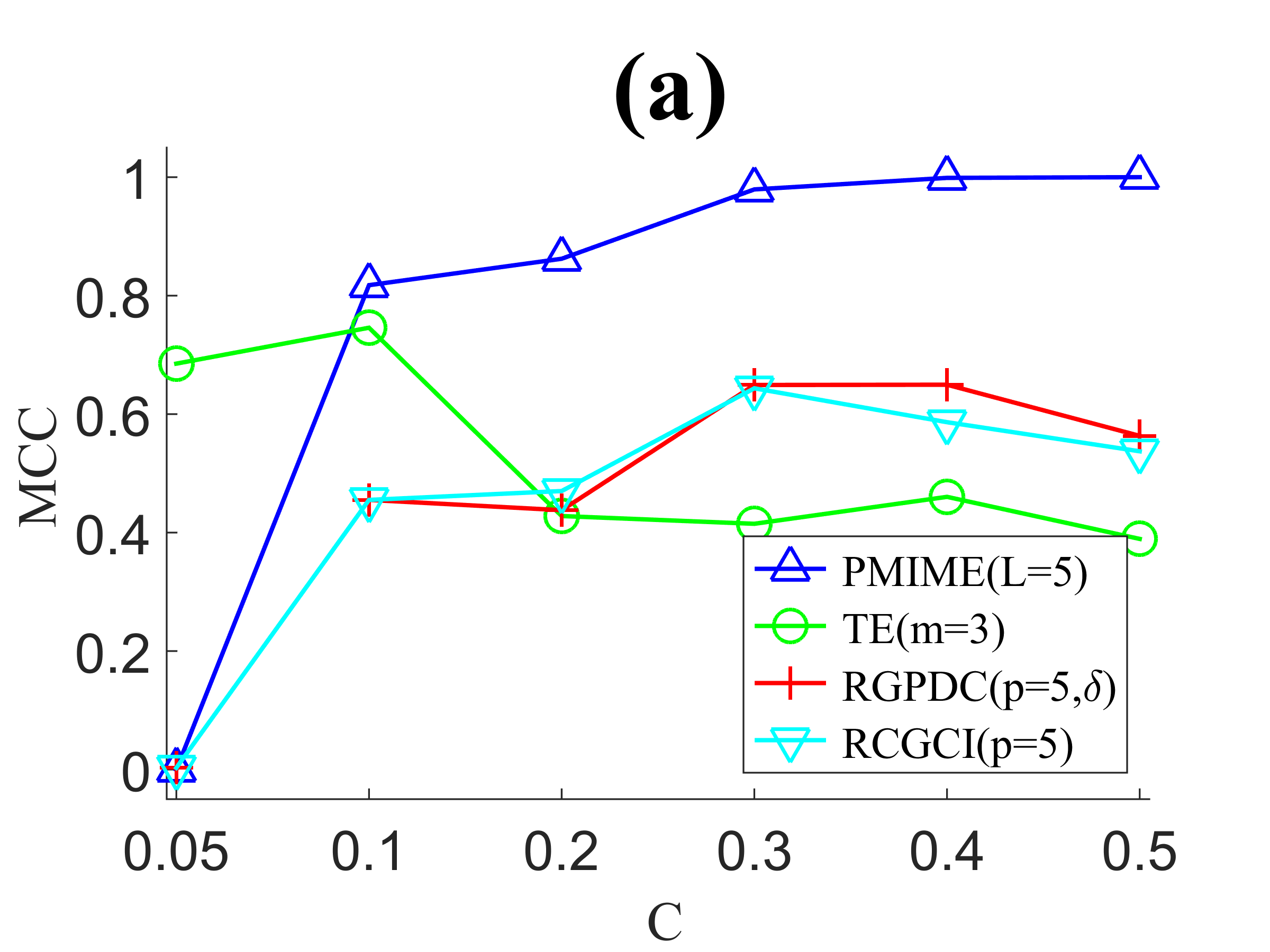
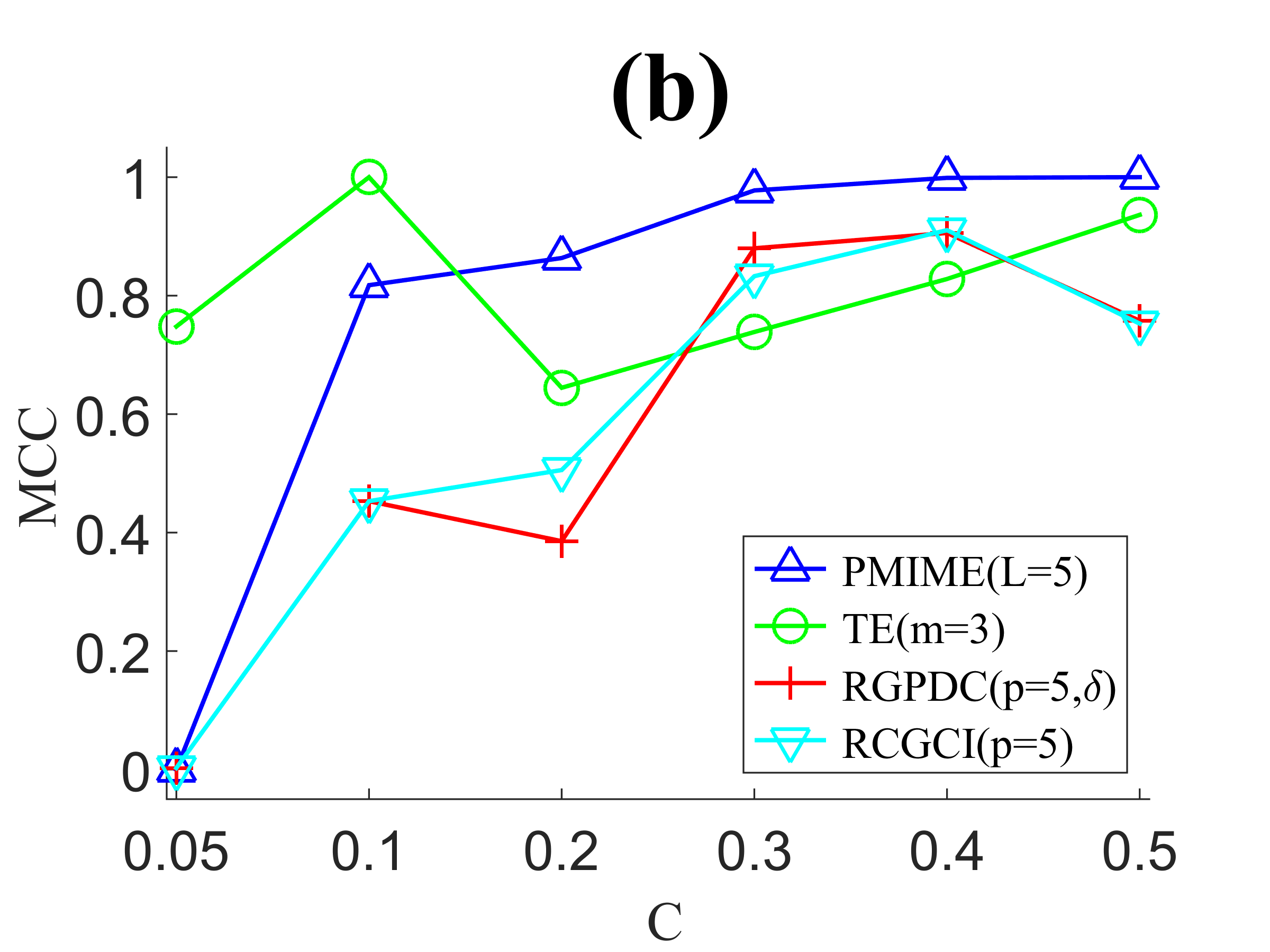
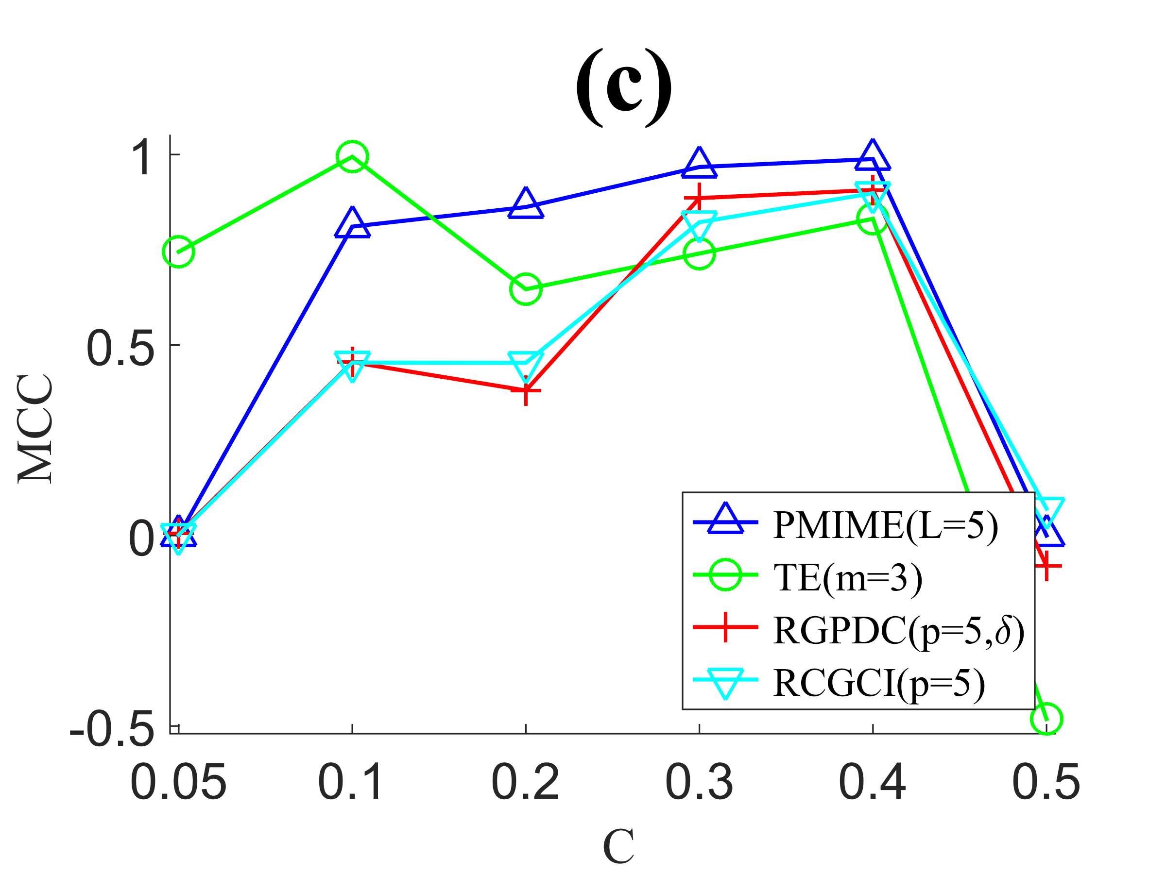
Figure 5: MCC of PMIME ($L\!=\!5$), TE ($m\!=\!3$), RGPDC ($p\!=\!5$,$\delta$), RCGCI ($p\!=\!5$) as a function of the coupling strength $C$ in system S1 of the coupled Hénon maps ($K\!=\!25$, $n\!=\!2048$) for the three significance criteria: (a) statistical testing at $\alpha\!=\!0.05$, (b) true density threshold $\rho_{0}\!=\!48$ and (c) magnitude threshold $th_{\rho_{0}}$.

The parameters in the criteria are $\alpha\!=\!0.05$ for the statistical testing, the true density of the original network $\rho_{0}\!=\!48$, and the average magnitude threshold $th_{\rho_{0}}$ over all magnitude thresholds corresponding to the true density for the 10 realizations. For all significance criteria, the PMIME exhibits the best performance for large $C>0.1$ while TE has the highest MCC for small $C$ at 0.05 and 0.1. Though S1 is a nonlinear system, the linear measures RCGCI and RGPDC (using the same dimension reduction step) are competitive and as good as or better than TE for large $C$. Thus for this system and setting of $n$, $K$ and large $C$, the rate of indirect (false) couplings found by the nonlinear bivariate measure TE is as large as or larger than the undetected nonlinear couplings from the linear measures RCGCI and RGPDC. This indicates that linear measures with dimension reduction may even perform better than nonlinear ones in settings of time series from nonlinear systems. It is noted that the coupling strength $C\!=\!0.05$ is very weak and the dimension reduction methods PMIME, RCGCI and RGPDC find no significant causal effects giving zero, which cannot change with any significance criterion. On the other hand, the small TE values for $C\!=\!0.05$ are still found significant at a good proportion giving rather large MCC at the level of 0.8.

3.3 Ranking of causality measures for each synthetic system

We derive summary results of all measures at each system over all coupling strengths $C$ and for different number of variables $K$ and time series lengths $n$ where applicable. For this, we use the average score index $s_{i,j}$ for each measure $i$ at each system $j$ as defined in Sec. 2.4. In all results in this section, the statistical significance testing for $\alpha\!=\!0.05$ has been used.

In Table 5, the average score $s_{i,j}$ for system S1 (coupled Hénon maps) is presented for the eight measures scoring highest at each scenario combining $K\!=\!5$ and $K\!=\!25$ with $n\!=\!512$ and $n\!=\!2048$.

Table 5: The ranking of the eight best measures according to the score index for system S1 of coupled Hénon maps for all scenarios of number of variables $K$ and time series length $n$.

$K\!=\!5$				$K\!=\!25$
$n\!=\!512$		$n\!=\!2048$		$n\!=\!512$		$n\!=\!2048$
Measure	Score	Measure	Score	Measure	Score	Measure	Score
PMIME($L\!=\!5$)	0.87	PMIME($L\!=\!5$)	0.84	PMIME($L\!=\!5$)	0.92	PMIME($L\!=\!5$)	0.91
TERV($m\!=\!3$)	0.78	RGPDC($p\!=\!5$,$\delta$)	0.77	TE($m\!=\!2$)	0.87	RGPDC($p\!=\!5$,$\delta$)	0.83
STE($m\!=\!3$)	0.77	RGPDC($p\!=\!5$,$\theta$)	0.76	TE($m\!=\!3$)	0.86	RGPDC($p\!=\!5$,$\theta$)	0.83
TE($m\!=\!3$)	0.72	RCGCI($p\!=\!5$)	0.76	RGPDC($p\!=\!5$,$\beta$)	0.81	RCGCI($p\!=\!5$)	0.82
RCGCI($p\!=\!5$)	0.71	RGPDC($p\!=\!5$,$\gamma$)	0.75	RGPDC($p\!=\!5$,$\alpha$)	0.81	RGPDC($p\!=\!5$,$\beta$)	0.82
RGPDC($p\!=\!5$,$\alpha$)	0.71	RGPDC($p\!=\!5$,$\beta$)	0.75	RGPDC($p\!=\!5$,$\theta$)	0.79	RGPDC($p\!=\!5$,$\alpha$)	0.81
CGCI($p\!=\!5$)	0.70	PDC($p\!=\!5$,$\alpha$)	0.75	RGPDC($p\!=\!5$,$\delta$)	0.78	RGPDC($p\!=\!5$,$\gamma$)	0.80
RGPDC($p\!=\!5$,$\gamma$)	0.70	GPDC($p\!=\!5$,$\alpha$)	0.73	RCGCI($p\!=\!5$)	0.77	CGCI($p\!=\!5$)	0.76

In all scenarios of S1 the PMIME measure is found to have the best performance. Also, the other measures of dimension reduction RCGCI and RGPDC reach highly ranked positions in all scenarios, especially in the case of large time series length. It is noted that these two measures are linear and they beat many other nonlinear measures showing the importance of proper dimension reduction. For small time series length ($n\!=\!512$), the information measures show better performance and it is again notable that the bivariate measures, such as TE, STE and TERV, score higher than the corresponding multivariate measures, PTE PSTE and PTERV. Again, the explanation for this lies in the inability of the multivariate measures to deal with high dimensions if dimension reduction is not employed. Having even as low as three conditioning variables in the conditional mutual information used by these measures (in the case of $K\!=\!25$ the three more correlated variables in terms of MI to the driving variable are selected from the 23 remaining variables) does not provide as accurate estimates of the causal effects as the respective bivariate measures. These multivariate measures (along other multivariate measures of no dimension reduction) give non-existing causal effects even to the beginning and end of the ring, whereas the respective bivariate measures do not, and only estimate additionally indirect causal effects (results not shown here).

In Table 6, the average score for system S2 of coupled Mackey-Glass subsystems is presented for the eight measures scoring highest at each scenario combining $K\!=\!5$ and $K\!=\!25$ with $\Delta\!=\!100$ and $\Delta\!=\!300$, where $\Delta$ controls the complexity of each subsystem.

Table 6: The ranking of the eight best measures according to the score index for system S2 of coupled Mackey-Glass subsystems for all scenarios of number of variables $K$ and delay parameter $\Delta$ that controls the complexity of each subsystem.

$K\!=\!5$				$K\!=\!25$
$\Delta\!=\!100$		$\Delta\!=\!300$		$\Delta\!=\!100$		$\Delta\!=\!300$
Measure	Score	Measure	Score	Measure	Score	Measure	Score
RGPDC($p\!=\!20$,$\alpha$)	0.90	RCGCI($p\!=\!20$)	0.88	PMIME($L\!=\!50$)	1.00	PMIME($L\!=\!50$)	0.95
RGPDC($p\!=\!20$,$\delta$)	0.88	RGPDC($p\!=\!20$,$\gamma$)	0.86	PGCI($p\!=\!5$)	0.87	RCGCI($p\!=\!5$)	0.89
RGPDC($p\!=\!20$,$\beta$)	0.88	RGPDC($p\!=\!20$,$\delta$)	0.86	RGPDC($p\!=\!20$,$\gamma$)	0.85	RGPDC($p\!=\!5$,$\delta$)	0.88
RGPDC($p\!=\!20$,$\gamma$)	0.88	RGPDC($p\!=\!20$,$\alpha$)	0.86	RGPDC($p\!=\!20$,$\delta$)	0.85	RGPDC($p\!=\!5$,$\gamma$)	0.87
RCGCI($p\!=\!20$)	0.86	RGPDC($p\!=\!20$,$\theta$)	0.85	RGPDC($p\!=\!20$,$\beta$)	0.84	RGPDC($p\!=\!5$,$\beta$)	0.86
RGPDC($p\!=\!20$,$\theta$)	0.86	RGPDC($p\!=\!20$,$\beta$)	0.85	RCGCI($p\!=\!20$)	0.84	RGPDC($p\!=\!5$,$\alpha$)	0.86
RGPDC($p\!=\!5$,$\theta$)	0.86	RGPDC($p\!=\!5$,$\gamma$)	0.80	RGPDC($p\!=\!20$,$\alpha$)	0.83	RGPDC($p\!=\!5$,$\theta$)	0.85
RGPDC($p\!=\!5$,$\delta$)	0.84	RCGCI($p\!=\!5$)	0.78	PGCI($p\!=\!20$)	0.82	RGPDC($p\!=\!20$,$\alpha$)	0.81

This system is comprised of highly complex systems with complexity increasing with $\Delta$. For $K\!=\!5$ and regardless of $\Delta$, the linear measures using dimension reduction RCGCI and RGPDC show the best performance, indicating again the importance of dimension reduction, here for oscillating complex systems. The PMIME scores slightly lower than these measures and given that RGPDC scores equally high at different bands, together with RCGCI they occupy the first eight places, so that the PMIME is not listed. For $K\!=\!25$ on the other hand, the PMIME scores much higher than the RCGCI and RGPDC measures and is at the first place for both $\Delta\!=\!100$ and $\Delta\!=\!300$. Apparently, the dimension reduction in the information measure of PMIME is more effective than in the VAR-based measure of RCGCI and RGPDC for larger $K$.

In Table 7, the average score for system S3 of the neural mass model is presented as for S2, but having as system parameter $A\!=\!3.45,3.7$, where the latter value indicates more clear oscillating behavior.

Table 7: The ranking of the eight best measures according to the score index for system S3 of the neural mass model for all scenarios of number of variables $K$ and oscillation controlling parameter $A$.

$K\!=\!5$				$K\!=\!25$
$A\!=\!3.45$		$A\!=\!3.7$		$A\!=\!3.45$		$A\!=\!3.7$
Measure	Score	Measure	Score	Measure	Score	Measure	Score
RCGCI($p\!=\!20$)	0.88	GPDC($p\!=\!20$,$\theta$)	0.94	GPDC($p\!=\!5$,$\theta$)	0.83	GPDC($p\!=\!20$,$\theta$)	0.92
GPDC($p\!=\!20$,$\theta$)	0.88	PDC($p\!=\!20$,$\theta$)	0.88	GPDC($p\!=\!20$,$\theta$)	0.82	CGCI($p\!=\!20$)	0.90
RGPDC($p\!=\!20$,$\alpha$)	0.88	PMIME($L\!=\!20$)	0.80	RCGCI($p\!=\!20$)	0.81	dDTF($p\!=\!20$,$\delta$)	0.89
RGPDC($p\!=\!20$,$\gamma$)	0.87	RGPDC($p\!=\!5$,$\alpha$)	0.78	RGPDC($p\!=\!20$,$\delta$)	0.79	GPDC($p\!=\!5$,$\alpha$)	0.87
PGCI($p\!=\!20$)	0.87	RCGCI($p\!=\!5$)	0.78	RGPDC($p\!=\!20$,$\beta$)	0.79	PMIME($L\!=\!20$)	0.87
CGCI($p\!=\!20$)	0.87	RGPDC($p\!=\!5$,$\alpha$)	0.77	RGPDC($p\!=\!20$,$\theta$)	0.79	PDC($p\!=\!5$,$\alpha$)	0.82
RGPDC($p\!=\!20$,$\theta$)	0.86	RGPDC($p\!=\!20$,$\theta$)	0.77	CGCI($p\!=\!20$)	0.78	PDC($p\!=\!20$,$\theta$)	0.80
RGPDC($p\!=\!20$,$\delta$)	0.85	RGPDC($p\!=\!20$,$\gamma$)	0.77	PDC($p\!=\!20$,$\theta$)	0.78	GPDC($p\!=\!20$,$\alpha$)	0.80

In all scenarios GPDC shows the best performance. The RCGCI measure for $A\!=\!3.45$ reaches the next position and also RGPDC reaches a high position on the ranking in the first three scenarios. The fact that GPDC scores higher than RGPDC also for $K\!=\!25$ indicates that for this system and both $A$ the inclusion of all lagged terms in VAR of order $p\!=\!5$ or $p\!=\!20$ gives somehow better identification of the correct couplings after significance testing. This is so, due to the relative large length $n\!=\!4096$ of the time series that allows for the reliable estimation of the coefficients being as many as $20\!\cdot\!25\!=\!500$. For $A\!=\!3.45$, the PMIME does not score high as its sensitivity is comparatively small (fails to find significant proportion of true causal effects), whereas for $A\!=\!3.7$ the PMIME is also among the first eight best measures. It is observed that in all settings the frequency measures, and particularly at low frequency bands, have the ability to identify the true causality interactions better than information and other measures. This is reasonable since this system is characterized by strongly harmonic oscillations.

For S4, no average results are shown as the system is run for only one scenario, and the ranking for this was shown in Table 4 and discussed earlier.

3.4 Overall ranking of causality measures

For an overall evaluation of the causality measures, the average score $s_{i}$ over all systems and scenarios is computed for each measure $i$, as defined in Sec. 2.4. In Table 8, the ten measures with highest score $s_{i}$ are listed.

Table 8: Average score index over all systems and scenarios.

Measure	Score
PMIME	0.80
RGPDC	0.79
RCGCI	0.78
GPDC	0.63
CGCI	0.61
PGCI	0.61
PDC	0.56
TE	0.51
dDTF	0.50
TERV	0.46

It is noted that for each measure computed for varying parameters, such as the frequency bands for the frequency measures, only the one with the highest score is listed. The best performance is achieved by the three measures making use of dimension reduction, with the information measure PMIME scoring highest. It is noted that there is a jump in score from the third to the fourth place, showing the superiority of the measures of dimension reduction over the other measures. The remaining places in the list are dominated by the linear measures in the time and frequency domain. Comparing the frequency measures based all on the same VAR model we note that GPDC, and even PDC score higher than dDTF. As for the information measures, the bivariate measures TE and TERV score much higher than the multivariate respective measures (results not shown), indicating the inability of multivariate information measures to perform well unless an appropriate dimension reduction is applied.

4 Discussion

In this paper, a simulation study is performed for the estimation of causality networks from multivariate time series. For the network construction, Granger causality measures, simply termed here as causality measures, of different type were employed as information and model-based measures, measures based on phase, frequency measures and measures making use of dimension reduction. These measures are applied to linear and nonlinear (chaotic), deterministic and stochastic, coupled simulated systems, to evaluate their ability to detect the existing coupled pairs of observed variables of these systems. We considered the nonlinear dynamical systems of coupled Hénon maps (S1), coupled Mackey-Glass subsystems (S2), the so-called neural mass model (S3), and a linear vector autoregressive process (VAR) of order 3 (S4). For systems S1, S2, S3 we used $K\!=\!5$ and $K\!=\!25$ subsystems, whereas S4 was defined only on $K\!=\!25$ variables. For S2 and S3, we considered two regimes of different complexity for each system, controlled by a system parameter. For S1, S2, and S3, a range of coupling strengths $C$ were designed covering the setting of none to weak and strong coupling. For S1, a small and a large time series length $n$ were used. This design of the simulation aimed at testing the causality measures on different types of systems with respect to time (S1, S4 are discrete and S2, S3 continuous in time), low and high dimensional having $K\!=\!5$ and $K\!=\!25$, linear (S4) and nonlinear (S1, S2, S3), deterministic (S1, S2) and stochastic (S3, S4), and for a range of coupling strengths (S1, S2, S3). Thus, rather than concentrating on a particular system or type of systems, e.g. often met in EEG studies, we aimed at evaluating the performance of the causality measures on many different system settings. Measures that were best suited for strongly oscillating systems, such as the frequency measures, may not be appropriate for maps, and on the other hand, information measures on ranks (such as TERV) that are more appropriate for discrete-time systems (maps) may not be appropriate for strongly oscillating signals. However, the evaluation showed that this was not the case, and, in the overall ranking, frequency measures dominated, but also TERV was included among the ten best.

The evaluation of the measures was based on the match of the causality network constructed from each measure to the original coupling network of the system generating the multivariate time series. For this, three significance criteria were used to transform the value of each causality measure, corresponding to a weighted network connection, to a binary value, corresponding to a binary connection. While the criteria of network density threshold and magnitude threshold are arbitrary and best results are only attained when the thresholds are given based on the knowledge of the original coupling network, the statistical testing, which does not require a-priori information on the underlying system, was competitive and was further suggested as the criterion of choice to derive binary connections. Performance indices were computed checking the preservation of the original binary connections (true) in the causality binary network (estimated), and we used the Matthews correlation coefficient (MCC) to quantify best the matching performance of each causality measure as it weighs sensitivity and specificity.

We considered bivariate and multivariate causality measures, and a subset of three multivariate measures making use of dimension reduction. The first is the information measure of partial mutual information from mixed embedding (PMIME), which can be considered as a restriction of the partial transfer entropy (PTE) to the most relevant lagged variables. The other two measures are linear and they are both based on VAR model. The dimension reduction suggests fitting a sparse VAR rather than a full VAR. While the conditional Granger causality index (CGCI) is defined in the time domain on the full VAR, the restricted CGCI (RCGCI) is computed on the sparse VAR, and accordingly in the frequency domain the generalized partial directed coherence (GPDC) is modified using a sparse VAR to the restricted GPDC (RGPDC).

While linear models can be estimated sufficiently well in high-dimensional time series, provided the length of the time series is much larger than the number of the unknown model coefficients, the estimation of entropies, used in information measures, in high dimension is problematic, even when using the most appropriate estimate of nearest neighbors. To make a fair comparison between the multivariate information measure making use of dimension reduction (PMIME) to the other multivariate information measures in high-dimensional time series (here $K\!=\!25$), for the latter measures we do not condition the causal relationship among the driving and response to all remaining variables (23 in our case), but rather select the three variables that are best correlated in terms of mutual information to the driving variable. In this way we avoid to some degree the curse of dimensionality, but still the embedding is done separately for each of the five variables, i.e. the driving, the response and the other three variables, whereas for the measures using dimension reduction, the embedding is built jointly for all variables selecting only the most appropriate lagged variables.

The evaluation of the causality measures showed differences in their performance in the different systems and their parameters ($n$, $K$, $C$ and system parameter $\Delta$ for S2 and $A$ for S3). For system S1, the measures making use of dimension reduction scored highest regardless of $n$ and $K$ with the PMIME attaining highest MCC for all but very small $C$. Bivariate information measures scored high here but only for small $n$. For system S2, the frequency measures were the most accurate at all frequency bands, especially for small $C$ while for stronger couplings dimension reduction measures reached higher MCC. For high-dimensional time series ($K\!=\!25$) again the PMIME scored highest followed mainly by the linear dimension reduction measures for different parameter values. For system S3 characterized by strong oscillations, the frequency measures performed best occupying the highest ranks and only the PMIME entered the list of eight highest rankings for the system parameter $A\!=\!3.7$ for both $K$. For the linear VAR system S4, as expected, the linear measures with dimension reduction performed best and the respective linear measures of full dimension had also increased performance.

The conclusions of the simulation study on comparatively low-dimensional ($K\!=\!5$) and high-dimensional ($K\!=\!25$) time series from different systems are itemized as follows:

1. The multivariate measures making use of dimension reduction (PMIME, RCGCI, RGPDC) outperform all other bivariate and multivariate measures.

2. Among the dimension reduction measures, the information measure of PMIME is overall best but the overall score is slightly higher than that of the other two linear measures. Though the PMIME outperforms the other measures in the chaotic systems S1 and S2, for the strongly oscillating stochastic system S3 and the linear stochastic process S4 it scores lower than RCGCI and RGPDC.

3. Linear measures, especially these applying dimension reduction, exhibited a competitive performance to other nonlinear measures also on nonlinear systems, such as S1, S2 and S3. This remark supports the use of linear measures (preferably with dimension reduction) to settings that may involve nonlinear relationships. Certainly, results still depend on the studied system.

4. Though bivariate measures tend to identify causality relationships that are not direct, they do not fail in identifying non-existing causal relationships. The latter occurs when using multivariate measures without dimension reduction. Though this effect cannot be captured by standard performance indices used in this study, such as the sensitivity and specificity, it is a significant finding advocating against the use of multivariate measures, unless dimension reduction is applied.

Admittedly, the collection of causality measures is biased including all measures our team has developed. On the other hand, the collection is not comprehensive, leaving out nonlinear measures that are more difficult to implement and could not be found freely available when the study was initiated. It is noted that initially, many connectivity measures that are not directional, especially these based on phases, were included, but they could not be fairly evaluated in the designed framework comparing the derived network to the original network of directed connections. The simulation study was conducted using four systems, leaving out other systems, such as the coupled Lorenz or coupled Rössler systems, as well as different coupling structures, such as the random (used here only in S4), small-world and scale-free, used by our team in other studies. Besides these shortcomings, we believe the current study can be useful for methodologists and practitioners to assess the strengths and weaknesses of the different causality measures and their applicability especially to high-dimensional time series.

Part of the research was supported by a grant from the Greek General Secretariat for Research and Technology (Aristeia II, No 4822).

References yes

References

- Arenas et al. (2008) Arenas, A.; Diaz-Guilera, A.; Kurths, J.; Moreno, Y.; Zhou, C. Synchronization in Complex Networks. Physics Reports 2008, 469, 93–153.
- Zanin et al. (2012) Zanin, M.; Sousa, P.; Papo, D.; Bajo, R.; García-Prieto, J.; Pozo, F.; Menasalvas, E.; Boccaletti, S. Optimizing Functional Network Representation of Multivariate Time Series. Scientific Reports 2012, 2, 630.
- Granger (1969) Granger, J. Investigating Causal Relations by Econometric Models and Cross-Spectral Methods. Acta Physica Polonica B 1969, 37, 424–438.
- Wiener (1956) Wiener, N. The theory of prediction. Modern Mathematics for Engineers; Beckenbach, E., Ed. McGraw-Hill, 1956.
- Smith et al. (2011) Smith, S.; Miller, K.; Salimi-Khorshidi, G.; Webster, M.; Beckmann, C.; Nichols, T.; Ramsey, J.; Woolrich, M. Network Modelling Methods for fMRI. Neuroimage 2011, 54, 875–891.
- Bastos and Schoffelen (2016) Bastos, A.; Schoffelen, J.M. A Tutorial Review of Functional Connectivity Analysis Methods and Their Interpretational Pitfalls. Frontiers in Systems Neuroscience 2016, 9.
- Porta and Faes (2016) Porta, A.; Faes, L. Wiener-Granger Causality in Network Physiology With Applications to Cardiovascular Control and Neuroscience. Proceedings of the IEEE 2016, 104, 282–309.
- Fornito et al. (2016) Fornito, A.; Zalesky, A.; Bullmore, E.T. Fundamentals of Brain Network Analysis, 1 ed.; Academic Press, Elsevier, 2016.
- Hlinka et al. (2011) Hlinka, J.; Hartman, D.; Vejmelka, M.; Runge, J.; Marwan, N.; Kurths, J.; Palus, M. Reliability of Inference of Directed Climate Networks Using Conditional Mutual Information. Entropy 2011, 15, 2023–2045.
- Dijkstra et al. (2019) Dijkstra, H.; Hernández-García, E.; Masoller, C.; Barreiro, M. Networks in Climate; Cambridge University Press: Cambridge, 2019.
- Schiff et al. (1996) Schiff, S.; So, P.; Chang, T.; Burke, R.; Sauer, T. Detecting Dynamical Interdependence and Generalized Synchrony through Mutual Prediction in a Neural Ensemble. Physical Review E 1996, 54, 6708–6724.
- Le Van Quyen et al. (1999) Le Van Quyen, M.; Martinerie, J.; Adam, C.; Varela, F.J. Nonlinear Analyses of Interictal EEG Map the Brain Interdependences in Human Focal Epilepsy. Physica D: Nonlinear Phenomena 1999, 127, 250–266.
- Chen et al. (2004) Chen, Y.; Rangarajan, G.; Feng, J.; Ding, M. Analyzing Multiple Nonlinear Time Series with Extended Granger Causality. Physics Letters A 2004, 324, 26–35.
- Faes et al. (2008) Faes, L.; Porta, A.; Nollo, G. Mutual Nonlinear Prediction as a Tool to Evaluate Coupling Strength and Directionality in Bivariate Time Series: Comparison among Different Strategies Based on Nearest Neighbors. Physical Review E 2008, 78, 026201.
- Marinazzo et al. (2006) Marinazzo, D.; Pellicoro, M.; Stramaglia, S. Nonlinear parametric model for Granger causality of time series. Physical Review E 2006, 73.
- Marinazzo et al. (2008) Marinazzo, D.; Pellicoro, M.; Stramaglia, S. Kernel Method for Nonlinear Granger Causality. Physical Review Letters 2008, 100, 144103.
- Marinazzo et al. (2011) Marinazzo, D.; Liao, W.; Chen, H.; Stramaglia, S. Nonlinear Connectivity by Granger Causality. NeuroImage 2011, 58, 330–338.
- Karanikolas and Giannakis (2017) Karanikolas, G.V.; Giannakis, G.B. Identifying Directional Connections in Brain Networks via Multi-kernel Granger Models. 2017 IEEE International Conference on Acoustics, Speech and Signal Processing (ICASSP), 2017, pp. 6304–6308.
- Montalto et al. (2015) Montalto, A.; Stramaglia, S.; Faes, L.; Tessitore, G.; Prevete, R.; Marinazzo, D. Neural Networks with Non-uniform Embedding and Explicit Validation Phase to Assess Granger Causality. Neural Networks 2015, 71, 159–171.
- Abbasvandi and Nasrabadi (2019) Abbasvandi, Z.; Nasrabadi, A.M. A Self-organized Recurrent Neural Network for Estimating the Effective Connectivity and its Application to EEG Data. Computers in Biology and Medicine 2019, 110, 93–107.
- Geweke (1982) Geweke, J. Measurement of Linear Dependence and Feedback Between Multiple Time Series. Journal of the American Statistical Association 1982, 77, 304–313.
- Geweke (1984) Geweke, J.F. Measures of Conditional Linear Dependence and Feedback between Time Series. Journal of the American Statistical Association 1984, 79, 907–915.
- Kaminski and Blinowska (1991) Kaminski, M.J.; Blinowska, K.J. A New Method of the Description of the Information Flow in the Brain Structures. Biological Cybernetics 1991, 65, 203–210.
- Baccalá and Sameshima (2001) Baccalá, L.; Sameshima, K. Partial Directed Coherence: a New Concept in Neural Structure Determination. Biological Cybernetics 2001, 84, 463–474.
- Arnhold et al. (1999) Arnhold, J.; Grassberger, P.; Lehnertz, K.; Elger, C.E. A Robust Method for detecting Interdependences: Application to Intracranially Recorded EEG. Physica D 1999, 134, 419–430.
- Romano et al. (2007) Romano, M.C.; Thiel, M.; Kurths, J.; Grebogi, C. Estimation of the Direction of the Coupling by Conditional Probabilities of Recurrence. Physical Review E 2007, 76, 036211.
- Schreiber (2000) Schreiber, T. Measuring Information Transfer. Physical Review Letters 2000, 85, 461–464.
- Palus (1996) Palus, M. Coarse-grained entropy rates for characterization of complex time series. Physica D:Nolinear Phenom. 1996, 93, 64–77.
- Vlachos and Kugiumtzis (2010) Vlachos, I.; Kugiumtzis, D. Non-uniform State Space Reconstruction and Coupling Detection. Physical Review E 2010, 82, 016207.
- Rosenblum and Pikovski (2001) Rosenblum, M.G.; Pikovski, A.S. Detecting Direction of Coupling in Interacting Oscillators. Physical Review E 2001, 64, 045202.
- Nolte et al. (2008) Nolte, G.; Ziehe, A.; Nikulin, V.V.; Schlögl, A.; Krämer, N.; Brismar, T.; Müller, K.R. Robustly Estimating the Flow Direction of Information in Complex Physical Systems. Physical Review Letters 2008, 100, 234101.
- Lehnertz et al. (2009) Lehnertz, K.; Bialonski, S.; Horstmann, M.T.; Krug, D.; Rothkegel, A.; Staniek, M.; Wagner, T. Synchronization Phenomena in Human Epileptic Brain Networks. Journal of Neuroscience Methods 2009, 183, 42–48.
- Rings and Lehnertz (2016) Rings, T.; Lehnertz, K. Distinguishing between Direct and Indirect Directional Couplings in Large Oscillator Networks: Partial or Non-partial Phase Analyses? Chaos 2016, 26.
- Han et al. (2016) Han, X.; Shen, Z.; Wang, W.X.; Lai, Y.C.; Grebogi, C. Reconstructing Direct and Indirect Interactions in Networked Public Goods Game. Scientific Reports 2016, 6.
- Blinowska et al. (2004) Blinowska, K.J.; Ku, R.; Kamiski, M. Granger Causality and Information Flow in Multivariate Processes. Physical Review E 2004, 50, 050902.
- Kus et al. (2004) Kus, R.; Kaminski, M.; Blinowska, K. Determination of EEG Activity Propagation: Pair-wise versus Multichannel Estimate. IEEE Transactions on Biomedical Engineering 2004, 51, 1501–1510.
- Eichler (2012) Eichler, M. Graphical modelling of multivariate time series. Probability Theory and Related Fields 2012, 153, 233–268.
- Marinazzo et al. (2012) Marinazzo, D.; Pellicoro, M.; Stramaglia, S. Causal Information Approach to Partial Conditioning in Multivariate Data Sets. Computational and Mathematical Methods in Medicine 2012, 2012.
- Faes et al. (2011) Faes, L.; Nollo, G.; Porta, A. Information-based Detection of Nonlinear Granger Causality in Multivariate Processes via a Nonuniform Embedding Technique. Physical Review E 2011, 83, 051112.
- Runge et al. (2012) Runge, J.; Heitzig, J.; Petoukhov, V.; Kurths, J. Escaping the Curse of Dimensionality in Estimating Multivariate Transfer Entropy. Physical Review Letters 2012, 108, 258701.
- Wibral et al. (2012) Wibral, M.; Wollstadt, P.; Meyer, U.; Pampu, N.; Priesemann, V.; Vicente, R. Revisiting Wiener’s Principle of Causality - Interaction-Delay Reconstruction Using Transfer Entropy and Multivariate Analysis on Delay-weighted Graphs. 2012 Annual International Conference of the IEEE Engineering in Medicine and Biology Society, 2012, pp. 3676–3679.
- Kugiumtzis (2013) Kugiumtzis, D. Direct Coupling Information Measure from Non-uniform Embedding. Physical Review E 2013, 87, 062918.
- Siggiridou and Kugiumtzis (2016) Siggiridou, E.; Kugiumtzis, D. Granger Causality in Multivariate Time Series Using a Time-Ordered Restricted Vector Autoregressive Model. IEEE Transactions on Signal Processing 2016, 64, 1759–1773.
- Smirnov and Andrzejak (2005) Smirnov, D.; Andrzejak, R. Detection of weak Directional Coupling: Phase-Dynamics Approach versus State-Space Approach. Physical Review E 2005, 71, 036207.
- Papana et al. (2011) Papana, A.; Kugiumtzis, D.; Larsson, P.G. Reducing the Bias of Causality Measures. Physical Review E 2011, 83, 036207.
- Silfverhuth et al. (2012) Silfverhuth, M.J.; Hintsala, H.; Kortelainen, J.; Seppanen, T. Experimental Comparison of Connectivity Measures with Simulated EEG Signals. Medical & Biological Engineering & Computing 2012, 50, 683–688.
- Fasoula et al. (2013) Fasoula, A.; Attal, Y.; Schwartz, D.; Ding, M.; Liang, H. Comparative Performance Evaluation of Data-Driven Causality Measures Applied to Brain Networks. Journal of Neuroscience Methods 2013, 215, 170–189.
- Papana et al. (2013) Papana, A.; Kyrtsou, C.; Kugiumtzis, D.; Diks, C. Simulation Study of Direct Causality Measures in Multivariate Time Series. Entropy 2013, 15, 2635–2661.
- Zaremba and Aste (2014) Zaremba, A.; Aste, T. Measures of Causality in Complex Datasets with Application to Financial Data. Entropy 2014, 16, 2309–2349.
- Cui and Li (2016) Cui, D.; Li, X. Multivariate EEG Synchronization Strength Measures. Signal Processing in Neuroscience; Li, X., Ed. Springer, 2016, pp. 235–259.
- Bakhshayesh et al. (2019) Bakhshayesh, H.; Fitzgibbon, S.P.; Janani, A.S.; Grummett, T.S.; Pope, K.J. Detecting Connectivity in EEG: A Comparative Study of Data-Driven Effective Connectivity Measures. Computers in Biology and Medicine 2019, 111, 103329.
- Blinowska (2011) Blinowska, K.J. Review of the Methods of Determination of Directed Connectivity from Multichannel Data. Medical & Biological Engineering & Computing 2011, 49, 521–529.
- Astolfi et al. (2005) Astolfi, L.; Cincotti, F.; Mattia, D.; Lai, M.; Baccala, L.; De Vico Fallani, F.; Salinari, S.; Ursino, M.; Zavaglia, M.; Babiloni, F. Comparison of Different Multivariate Methods for the Estimation of Cortical Connectivity: Simulations and Applications to EEG Data. 2005 IEEE Engineering in Medicine and Biology 27th Annual Conference, 2005, pp. 4484–4487.
- Florin et al. (2011) Florin, E.; Gross, J.; Pfeifer, J.; Fink, G.; Timmermann, L. Reliability of Multivariate Causality Measures for Neural Data. Journal of Neuroscience Methods 2011, 198, 344–358.
- Wu et al. (2011) Wu, M.H.; Frye, R.E.; Zouridakis, G. A Comparison of Multivariate Causality based Measures of Effective Connectivity. Computers in Biology and Medicine 2011, 21, 1132–1141.
- Sommariva et al. (2019) Sommariva, S.; Sorrentino, A.; Piana, M.; Pizzella, V.; Marzetti, L. A Comparative Study of the Robustness of Frequency-Domain Connectivity Measures to Finite Data Length. Brain Topography 2019, 32, 675–695.
- Diks and Fang (2017) Diks, C.; Fang, H. Transfer Entropy for Nonparametric Granger Causality Detection: An Evaluation of Different Resampling Methods. Entropy 2017, 19.
- Papana et al. (2017) Papana, A.; Kyrtsou, C.; Kugiumtzis, D.; Diks, C. Assessment of Resampling Methods for Causality Testing: A Note on the US Inflation Behavior. PLoS ONE 2017, 12.
- Moharramipour et al. (2018) Moharramipour, A.; Mostame, P.; Hossein-Zadeh, G.A.; Wheless, J.; Babajani-Feremi, A. Comparison of Statistical Tests in Effective Connectivity Analysis of ECoG Data. Journal of Neuroscience Methods 2018, 308, 317–329.
- Siggiridou et al. (2015) Siggiridou, E.; Koutlis, C.; Tsimpiris, A.; Kimiskidis, V.K.; Kugiumtzis, D. Causality Networks from Multivariate Time Series and Application to Epilepsy. 2015 37th Annual International Conference of the IEEE Engineering in Medicine and Biology Society (EMBC), 2015, pp. 4041–4044.
- Cui et al. (2008) Cui, J.; Xu, L.; Bressler, L.; Ding, M.; Liang, H. BSMART: A Matlab/C Toolbox for Analysis of Multichannel Neural Time Series. Neural Networks 2008, 21, 1094–1104.
- Seth (2010) Seth, A.K. A MATLAB Toolbox for Granger Causal Connectivity Analysis. Journal of Neuroscience Methods 2010, 186, 262 – 273.
- Niso et al. (2013) Niso, G.; Bruña, R.; Pereda, E.; Gutiérrez, R.; Bajo, R.; Maesté, F.; Del-Pozo, F. HERMES: Towards an Integrated Toolbox to Characterize Functional and Effective Brain Connectivity. Neuroinformatics 2013, 11, 405–434.
- Lizier (2014) Lizier, J. JIDT: An Information-Theoretic Toolkit for Studying the Dynamics of Complex Systems. Frontiers in Robotics and AI 2014, 1.
- Barnett and Seth (2014) Barnett, L.; Seth, K.A. The MVGC Multivariate Granger Causality Toolbox: A New Approach to Granger-Causal Inference. Journal of Neuroscience Methods 2014, 223, 50–68.
- Montalto et al. (2014) Montalto, A.; Faes, L.; Marinazzo, D. MuTE: A MATLAB Toolbox to Compare Established and Novel Estimators of the Multivariate Transfer Entropy. PLoS ONE 2014, 9.
- Lachaux et al. (1999) Lachaux, J.P.; Rodriguez, E.; Martinerie, J.; Varela, F.J. Measuring Phase Synchrony in Brain Signals. Human Brain Mapping 1999, 8, 194–208.
- Stam et al. (2007) Stam, C.J.; Nolte, G.; Daffertshofer, A. Phase Lag Index: Assessment of Functional Connectivity from Multi Channel EEG and MEG with Diminished Bias from Common Sources. Human Brain Mapping 2007, 28, 1178–1193.
- Vinck et al. (2011) Vinck, M.; Oostenveld, R.; Van Wingerden, M.; Battaglia, F.; Pennartz, C.M.A. An Improved Index of Phase-Synchronization for Electrophysiological Data in the Presence of Volume-Conduction, Noise and Sample-Size Bias. Neuroimage 2011, 55, 1548–1565.
- Tass et al. (1998) Tass, P.; Rosenblum, M.G.; Weule, J.; Kurths, J.; Pikovsky, A.; Volkmann, J.; Schnitzler, A.; Freund, H.J. Detection of n:m Phase Locking from Noisy Data: Application to Magnetoencephalography. Physical Review Letters 1998, 81, 3291–3294.
- Mormann et al. (2000) Mormann, F.; Lehnertz, K.; David, P.; Elger, C.E. Mean Phase Coherence as a Measure for Phase Synchronization and its Application to the EEG of Epilepsy Patients. Physica D 2000, 144, 358–369.
- Guo et al. (2008) Guo, S.; Seth, A.K.; Kendrick, K.; Zhou, C.; Feng, J. Partial Granger Causality – Eliminating Exogenous Inputs and Latent Variables. Journal of Neuroscience Methods 2008, 172, 79–93.
- Hatemi-J and Hacker (2012) Hatemi-J, A.; Hacker, R.S. Can the LR Test Be Helpful in Choosing the Optimal Lag Order in the VAR Model when Information Criteria Suggest Different Lag Orders?. Applied Economics 2009, 41, 1121-1125.
- Bruns and Stern (2019) Bruns, S. B; Stern, D. I. Lag Length Selection and P-hacking in Granger Causality Testing: Prevalence and Performance of Meta-regression Models. Empirical Economics 2019, 56, 797-830.
- Papana et al. (2012) Papana, A.; Kugiumtzis, D.; Larsson, P.G. Detection of Direct Causal Effects and Application in the Analysis of Electroencephalograms from Patients with Epilepsy. International Journal of Bifurcation and Chaos 2012, 22, 1250222.
- Staniek and Lehnertz (2008) Staniek, M.; Lehnertz, K. Symbolic Transfer Entropy. Physical Review Letters 2008, 100.
- Papana et al. (2015) Papana, A.; Kyrtsou, C.; Kugiumtzis, D.; Diks, C. Detecting Causality in Non-stationary Time Series Using Partial Symbolic Transfer Entropy: Evidence in Financial Data. Computational Economics 2015, pp. 1–25. doi:\changeurlcolorblack10.1007/s10614-015-9491-x.
- Kugiumtzis (2012) Kugiumtzis, D. Transfer Entropy on Rank Vectors. Journal of Nonlinear Systems and Applications 2012, 3, 73–81.
- Kugiumtzis (2013) Kugiumtzis, D. Partial Transfer Entropy on Rank Vectors. European Physical Journal Special Topics 2013, 222, 401–420.
- Baccala et al. (2007) Baccala, L.A.; Sameshima, K.; Takahashi, D.Y. Generalized Partial Directed Coherence. 2007 15th International Conference on Digital Signal Processing, 2007, pp. 163–166.
- Korzeniewska et al. (2003) Korzeniewska, A.; Manczak, M.and Kaminski, M.; Blinowska, K.; Kasicki, S. Determination of Information Flow Direction between Brain Structures by a Modified Directed Transfer Function Method (dDTF). Journal of Neuroscience Methods 2003, 125, 195–207.
- Hu et al. (2011) Hu, S.; Dai, G.; Worrell, G.A.; Dai, Q.; Liang, H. Causality Analysis of Neural Connectivity: Critical Examination of Existing Methods and Advances of New Methods. IEEE Transactions on Neural Networks 2011, 22, 829–844.
- Siggiridou et al. (2017) Siggiridou, E.; Kimiskidis, V.K.; Kugiumtzis, D. Dimension Reduction of Frequency-Based Direct Granger Causality Measures on Short Time Series. Journal of Neuroscience Methods 2017, 289, 64–74.
- Quian Quiroga et al. (2002) Quian Quiroga, R.; Kreuz, T.; Grassberger, P. Event Synchronization: A Simple and Fast Method to Measure Synchronicity and Time Delay Patterns. Physical Review E 2002, 66, 041904.
- Paluš et al. (2001) Paluš, M.; Komárek, V.; Hrncír, Z.; Šterbová, K. Synchronization as adjustment of information rates: detection from bivariate time series. Physical Review E 2001, 63, 046211.
- Verdes (2005) Verdes, P. Assessing causality from multivariate time series. Phys. Rev. E 2005, 72, 026222.
- Vakorin et al. (2009) Vakorin, V.A.; Krakovska, O.A.; McIntosh, A.R. Confounding Effects of Indirect Connections on Causality Estimation. Journal of Neuroscience Methods 2009, 184, 152–160.
- Paluš and Stefanovska (2003) Paluš, M.; Stefanovska, A. Direction of Coupling from Phases of Interacting Oscillators: An Information-Theoretic Approach. Physical Review E 2003, 67, 055201.
- Chicharro and Andrzejak (2009) Chicharro, D.; Andrzejak, R. Reliable Detection of Directional Couplings Using Rank Statistics. Physical Review E 2009, 80, 026217.
- Sugihara et al. (2012) Sugihara, G.; May, R.; Ye, H.; Hsieh, C.; Deyle, E.; Fogarty, M.; Munch, S. Detecting Causality in Complex Ecosystems. Science 2012, 338, 496–500.
- Yu and Huang (2001) Yu, G.H.; Huang, C.C. A Distribution Free Plotting Position. Stochastic Environmental Research and Risk Assessment 2001, 15, 462 – 476.
- Benjamini and Hochberg (1995) Benjamini, Y.; Hochberg, Y. Controlling the False Discovery Rate: A Practical and Powerful Approach to Multiple Testing. Journal of the Royal Statistical Society. Series B (Methodological) 1995, 57, 289–300.
- Matthews (1975) Matthews, B.W. Comparison of the Predicted and Observed Secondary Structure of T4 Phage Lysozyme. Biochimica et Biophysica Acta 1975, 405, 442–451.
- Lansdown (1998) Lansdown, F. Ordinal Ranking Methods for Multicriterion Decision Making. Naval Research Logistics (NRL) 1998, 43, 613–627.
- Kugiumtzis (2013) Kugiumtzis, D. Direct-Coupling Information Measure from Nonuniform Embedding. Physical Review E 2013, 87, 062918.
- Senthilkumar et al. (2008) Senthilkumar, D.V.; Lakshmanan, M.; Kurths, J. Transition from Phase to Generalized Synchronization in Time-Delay Systems. Chaos: An Interdisciplinary Journal of Nonlinear Science 2008, 18, 023118.
- Wendling et al. (2000) Wendling, F.; Bellanger, J.; Bartolomei, F.; Chauvel, P. Relevance of Nonlinear Lumped-Parameter Models in the Analysis of Depth-EEG Epileptic Signals. Biological Cybernetics 2000, 83, 367–378.
- Koutlis and Kugiumtzis (2016) Koutlis, C.; Kugiumtzis, D. Discrimination of Coupling Structures Using Causality Networks from Multivariate Time Series. Chaos: An Interdisciplinary Journal of Nonlinear Science 2016, 26.
- Basu and Michailidis (2015) Basu, S.; Michailidis, G. Regularized Estimation in Sparse High-Dimensional Time Series Models. Annals of Statistics 2015, 43, 1535–1567.
- Kugiumtzis (1996) Kugiumtzis, D. State Space Reconstruction Parameters in the Analysis of Chaotic Time Series - the Role of the Time Window Length. Physica D 1996, 95, 13–28.