Entropy of higher dimensional topological dS black holes with nonlinear source

Abstract

On the basis of the first law of black hole thermodynamics, we propose the concept of effective temperature of de Sitter(dS) black holes and conjecture that the effective temperature should be the temperature of the dS black holes when the Hawking radiation temperatures of the black hole horizon and the cosmological horizon are equal. Choosing different independent variables, we can find a differential equation satisfied by the entropy of the dS black hole. It is shown that the differential equation of entropy is independent of the choice of independent variables. From the differential equation, we get the entropy of dS black hole and other effective thermodynamic quantities. We also discuss the influence of several parameters on the effective thermodynamic quantities.

I Introduction

Recent years, the studies on the thermodynamic properties of black holes have made some progress. Firstly, Based on the fact that black hole satisfies the first law of thermodynamics, one corresponded the cosmological constant in AdS spacetime to the pressure in general thermodynamics, and got the extended first law of thermodynamics of black holes. Various critical phenomena of black holes in AdS spacetime have been extensively studied by comparing the equation of state of black hole with the van der Waals equation . One can further study the critical point and critical index of the AdS black holes, and discussed the influence of the parameters in spacetime on the phase transition 1 ; 2 ; 3 ; 4 ; 5 ; 6 ; 7 ; 8 ; 9 ; 10 ; 11 ; 12 ; 13 ; 14 ; 15 ; 16 ; 17 ; 18 ; 19 ; 20 ; 21 ; 22 ; 23 ; 24 ; 25 ; 26 .

For de Sitter spacetime, thermodynamic quantities of black hole horizon and cosmological horizon satisfies with the first law of thermodynamics respectively 27 ; 28 . However, the Hawking radiation temperature of two horizons are not equal in general cases +1 ; +2 ; +3 ; +4 ; +7 ; 29 ; 30 ; 31 ; 32 , thus the de Sitter black holes does not meet the requirement of stability of the thermodynamic equilibrium. This limited the research on the thermodynamical properties of the de Sitter black holes. Recent years, with the in-depth study of dark energy, the thermodynamical properties of de Sitter black holes aroused people’s attention 35 ; 36 ; 37 ; 38 ; 39 ; 40 . Because during the inflation in the very early period, our Universe was a quasi-de Sitter spacetime, and the cosmological constant introduced in the de Sitter spacetime is the contribution of vacuum energy, which is also a kind of matter energy. If the cosmological constant is just the dark energy, our Universe will evolve to a new de Sitter phase +8 ; +9 . For constructing the whole history of evolution of the Universe, it’s necessary to understand both the classical and quantum properties of the de Sitter spacetime. People usually define the entropy of de Sitter spacetime as the sum of two horizon’s entropies 29 ; 32 ; 35 ; 36 ; 37 . However, there is no theoretical proof supports this consequence.

Reviewing the four laws of thermodynamics found by Hawking and Bekenstein etc., 41 ; 42 ; 43 ; 44 ; 45 , and given the Hawking radiation temperature of black hole, the equation of state of black hole satisfy the first law of thermodynamics. By comparing the such a equation with the general thermodynamics system, they got the famous conclusion that the entropy of black hole equals quarter area of black hole horizon. Using this approach to the de Sitter spacetime one can get the same conclusion, i.e. the entropy of black hole horizon and the cosmological horizon are quarter of their corresponding area respectively. But some thermodynamic quantities in two horizons are same, such as energy, charge etc., which means two horizons are not independent. Entropy is usually related to the numbers of microscopic states. Although the microscopic origin of black hole entropy is still unclear, it must exist. For black holes with multiple horizons, such as SdS black hole, the black hole horizon and the cosmological horizon are in fact not independent. There may exist some correlations between them. The size of black hole horizon is closely related to the size of the cosmological horizon, and the evolution of black hole horizon will lead to the evolution of the cosmological horizon. Taking the correlations between the horizons into account, the total numbers of microscopic states are not simply the product of those of the two horizons (it will be, if the two horizons are isolated). Therefore, the total entropy is no longer the sum of the entropies of the two horizons, but should include an extra term coming from the contribution of the correlations of the two horizons.

In order to further study the thermodynamic properties of de Sitter black holes, we need to define its temperature and entropy. In this work, based on the consideration of dimension, we set the entropy of de Sitter black holes has the form of function $F_{n}(x)$. (here $x=r_{+}/r_{c}$ and $r_{+},r_{c}$ are positions of the black hole horizon and the cosmological horizon). Through the basic condition that the thermodynamic quantities of spacetime satisfy the first law of thermodynamics, and the relation between the effective temperature of spacetime and the radiation temperature of two horizons, we can find the differential equation for $F_{n}(x)$. As the black hole horizon of spacetime approaches to zero and de Sitter black hole approaches to the pure de Sitter one, and regard these as the initial conditions, the differential equation can be solved and the result is just the entropy. Furthermore, we can get the effective temperature and pressure etc. In order to make the discussion more general, we focus on the higher dimensional topological de Sitter black holes with nonlinear source (HDBRN) spacetime.

This paper is organized as follows. In Sect. 2, the corresponding thermodynamic quantities of black hole horizon and the cosmological horizon in the HDBRN spacetime will be introduced. And the condition obeyed by spacetime charge $Q$, when the radiation temperature of two horizons equal to each other. In Sect. 3, on the basis of considering the relation between two horizons, we give the entropy of HDBRN spacetime which satisfies the first law of thermodynamics as well as the effective temperature and pressure. Our conclusions are presented in Sect. 4.(we use the units $G=\hbar=k_{B}=c=1$)

II Topological black hole with nonlinear source

The$(n+1)-$dimensional action of Einstein gravity of nonlinear electrodynamics is 47 ; 48 :

$${I_{G}}=-\frac{1}{{16\pi}}\int_{M}{{d^{n+1}}x\sqrt{-g}[R-2\Lambda+L(F)]}-\frac{1}{{8\pi}}\int_{\partial M}{{d^{n}}x\sqrt{-\gamma}}\Theta(\gamma)$$ (1)

where $R$ is the scalar curvature, $\Lambda$ is the cosmological constant. In this action,

$${L}(F)=-F+\alpha{F^{2}}+o({\alpha^{2}}),$$ (2)

is the Lagrangian of nonlinear electrodynamics. $F={F_{\mu\nu}}{F^{\mu\nu}}$ is the Maxwell invariant, in which ${F_{\mu\nu}}={\partial_{\mu}}{A_{\nu}}-{\partial_{\nu}}{A_{\mu}}$ is the electromagnetic field tensor and $A_{\nu}$ is the gauge potential. In addition, $\alpha$ denotes nonlinearity parameter which is small, so the effects of nonlinearity can be considered as a perturbation.

The $n+1$ -dimensional topological black hole solutions can take the form of

$$ds^{2}=-f(r)d{t^{2}}+\frac{{d{r^{2}}}}{{f(r)}}+{r^{2}}d\Omega_{n-1}^{2},$$ (3)

where

$$f(r)=k-\frac{m}{{{r^{n-2}}}}-\frac{{2\Lambda{r^{2}}}}{{n(n-1)}}+\frac{{2{q^{2}}}}{{(n-1)(n-2){r^{2n-4}}}}-\frac{{4{q^{4}}\alpha}}{{(3{n^{7}}-7n+4){r^{2n-6}}}},$$ (4)

m is an integration constant which is related to the mass of the black hole and the last term of Eq. (4) indicates the effect of nonlinearity. The asymptotical behavior of the solution is AdS or dS provided $\Lambda<0$ or $\Lambda>0$, and the case of asymptotically flat solution is permitted for $\Lambda=0$ and $k=1$.

When $\Lambda>0$, the position of the spacetime black hole horizon $r_{+}$ and the universal horizon $r_{c}$ is satisfied with the equation $f({r_{+,c}})=0$. The radiation temperature of the two horizon can be written as follows 28 ; 47

$${T_{+}}=\frac{{f^{\prime}({r_{+}})}}{{4\pi}}=\frac{1}{{2\pi(n-1)}}\left({\frac{{(n-1)(n-2)k}}{{2{r_{+}}}}-\Lambda{r_{+}}-\frac{{{q^{2}}}}{{r_{+}^{2n-3}}}+\frac{{2{q^{4}}\alpha}}{{r_{+}^{4n-5}}}}\right).$$ (5)

$${T_{c}}=-\frac{{f^{\prime}({r_{c}})}}{{4\pi}}=-\frac{1}{{2\pi(n-1)}}\left({\frac{{(n-1)(n-2)k}}{{2{r_{c}}}}-\Lambda{r_{c}}-\frac{{{q^{2}}}}{{r_{c}^{2n-3}}}+\frac{{2{q^{4}}\alpha}}{{r_{c}^{4n-5}}}}\right).$$ (6)

The mass of the black hole is

$$M=\frac{{{V_{n-1}}(n-1)}}{{16\pi}}\left(\begin{array}[]{c}{kr_{+}^{n-2}-\frac{{2\Lambda r_{+}^{n}}}{{n(n-1)}}+\frac{{2{q^{2}}}}{{(n-1)(n-2)r_{+}^{n-2}}}-}\\ {\frac{{4{q^{4}}\alpha}}{{[2(n-2)(n+2)+(n-3)(n-4)]r_{+}^{3n-4}}}}\end{array}\right),$$ (7)

or

$$M=\frac{{{V_{n-1}}(n-1)}}{{16\pi}}\left(\begin{array}[]{c}{kr_{c}^{n-2}-\frac{{2\Lambda r_{c}^{n}}}{{n(n-1)}}+\frac{{2{q^{2}}}}{{(n-1)(n-2)r_{c}^{n-2}}}-}\\ {\frac{{4{q^{4}}\alpha}}{{[2(n-2)(n+2)+(n-3)(n-4)]r_{c}^{3n-4}}}}\end{array}\right),$$ (8)

where ${V_{n-1}}:=\frac{{2{\pi^{n/2}}}}{{\Gamma(n/2)}},{S_{+,c}}:=\frac{{{V_{n-1}}r_{+,c}^{n-1}}}{4},{V_{+,c}}:=\frac{{{V_{n-1}}r_{+,c}^{n}}}{n},Q:=\frac{q}{{4\pi}}{V_{n-1}},{\Phi_{+,c}}:=\frac{q}{{(n-2)r_{+,c}^{n-2}}}-\frac{{4{q^{3}}\alpha}}{{(3n-4)r_{+,c}^{3n-4}}},P:=-\frac{\Lambda}{{8\pi}},M:=\frac{{{V_{n-1}}(n-1)m}}{{16\pi}}.$

The thermodynamic quantity corresponding to the two horizons satisfies the first law of thermodynamics

$$dM={T_{+,c}}d{S_{+,c}}+{\Phi_{+,c}}dQ+{V_{+,c}}dP.$$ (9)

From the equation $f({r_{+,c}})=0,$ one can obtain

$$\frac{{2\Lambda}}{{n(n-1)}} = \frac{{k(1-{x^{n-2}})}}{{r_{c}^{2}(1-{x^{n}})}}-\frac{{2{q^{2}}(1-{x^{n-2}})}}{{(n-1)(n-2)r_{c}^{2n-2}{x^{n-2}}(1-{x^{n}})}}$$

$$+{\frac{{4{q^{4}}\alpha(1-{x^{3n-4}})}}{{[2(n-2)(n+2)+(n-3)(n-4)]r_{c}^{4n-4}{x^{3n-4}}(1-{x^{n}})}}},$$

$$M = \frac{{{V_{n-1}}(n-1)}}{{16\pi(1-{x^{n}})}}r_{c}^{n-2}{k({x^{n-2}}-{x^{n}})}+\frac{{2{q^{2}}}}{{(n-1)(n-2)r_{c}^{2(n-2)}}}\frac{{(1-{x^{2n-2}})}}{{{x^{n-2}}}}$$ (11)

$${-\frac{{4{q^{4}}\alpha}}{{[2(n-2)(n+2)+(n-3)(n-4)]r_{c}^{2(2n-3)}}}\frac{{(1-{x^{4n-4}})}}{{{x^{3n-4}}}}},$$

where $x=r_{+}/r_{c}$. When $T_{+}=T_{c}$, by solving Eq (5) and Eq (6), we can get

$$\Lambda=\frac{{(n-1)(n-2)k}}{{2r_{c}^{2}x}}-\frac{{{q^{2}}}}{{r_{c}^{2n-2}{x^{2n-3}}}}\frac{{1+{x^{2n-3}}}}{{(1+x)}}+\frac{{2{q^{4}}\alpha}}{{r_{c}^{4n-4}{x^{4n-5}}}}\frac{{1+{x^{4n-5}}}}{{(1+x)}}.$$ (12)

From Eq II) and Eq (12), one can find when $T_{+}=T_{c}$, one can obtain the following equation

$${l}\frac{{4{q^{4}}\alpha}}{{r_{c}^{4n-5}}}(n-2)\frac{{(3{n^{2}}-7n+4)(1-{x^{n}})(1+{x^{4n-5}})-n(n-1){x^{n-1}}(1-{x^{3n-4}})(1+x)}}{{(3{n^{2}}-7n+4){x^{2n-2}}}}$$ (13)

$$= \frac{{k(n-1)(n-2)(1+x){x^{2n-4}}}}{{{r_{c}}}}[nx(1-{x^{n-2}})-(n-2)(1-{x^{n}})]$$

$$-\frac{{2{q^{2}}}}{{r_{c}^{2n-3}}}[n{x^{n-1}}(1+x)(1-{x^{n-2}})-(n-2)(1-{x^{n}})(1+{x^{2n-3}})].$$

The Eq. (13) can be rewritten as

$$\frac{{4{q^{4}}\alpha}}{{r_{c}^{4n-6}}}{B_{1}}(x,n)=k{A_{1}}(x,n)+\frac{{2{q^{2}}}}{{r_{c}^{2n-4}}}{C_{1}}(x,n).$$ (14)

We can find that Eq. (14) is a function relation between the $\frac{{4{q^{4}}\alpha}}{{r_{c}^{4n-6}}}$, $\frac{{2{q^{2}}}}{{r_{c}^{2n-4}}}$and $k$, and any one of these can be a function of other two independent variables. When regard $\frac{{2{q^{2}}}}{{r_{c}^{2n-4}}}$as a function of $\frac{{4{q^{4}}\alpha}}{{r_{c}^{4n-6}}}$and $k$ , and substituted Eq. (12) and Eq. (13) into Eq. (5) or Eq. (6), thus when the two horizon radiation temperature satisfied the relation $T_{+}=T_{c}$, one can obtain

$$T = {T_{c}}={T_{+}}$$ (15)

$$= \frac{1}{{2\pi(n-1){r_{c}}K(x,n)}}\{k(n-2)(n-1)[n{x^{n-2}}(1-{x^{2}})(1-{x^{n-2}})-(1-{x^{n}})(1-{x^{2n-4}})]$$

$$+\frac{{(1-{x^{2n-2}})}}{{(3{n^{2}}-7n+4){x^{3n-4}}}}\frac{{4{q^{4}}\alpha}}{{r_{c}^{4n-6}}}[4{x^{n-2}}(1-{x^{n}})+n(1-11{x^{n-2}}+11{x^{2n-2}}-{x^{3n-4}})$$

$$-2{n^{2}}(1-{x^{3n-4}}+5{x^{2n-2}}-5{x^{n-2}})+{n^{3}}(1-{x^{3n-4}}-3{x^{n-2}}+3{x^{2n-2}})]\},$$

with

$$K(x,n)=[n{x^{n-1}}(1+x)(1-{x^{n-2}})-(n-2)(1-{x^{n}})(1+{x^{2n-3}})].$$ (16)

When set $n=3,\alpha=0,$ the spacetime will return to RN-de Sitter spacetime, one can obtain the effective temperature

$$T = {T_{c}}={T_{+}=}\frac{k}{2\pi r_{c}}\frac{3x(1-x^{2})(1-x)-(1-x^{3})(1-x^{2})}{3x^{2}(1+x)(1-x)-(1-x^{3})(1+x^{3})}$$

$$= \frac{k}{2\pi r_{c}}\frac{1-x}{(1+x)^{2}},$$

which is as same as the result mentioned by Ref 30 ; 31 ; cai .

When $\frac{{4{q^{4}}\alpha}}{{r_{c}^{4n-6}}}$ is regarded as the function of $\frac{{2{q^{2}}}}{{r_{c}^{2n-4}}}$and $k$, in the same way as above mentioned, we can get the following equation

$$T = {T_{c}}={T_{+}}=\frac{1}{{2\pi(n-1){r_{c}}(3{n^{2}}-7n+4)\tilde{K}(x,n)}}{(n-1)(n-2)k}$$ (18)

$${4(1-{x^{n}})(1-{x^{4n-6}})}+n[-7(1+{x^{5n-6}})-3{x^{n-2}}(1+{x^{3n-2}})+10{x^{n}}(1+{x^{3n-6}})]$$

$$+{n^{2}}[5{x^{n-2}}(1+{x^{3n-2}})-8{x^{n}}(1+{x^{3n-6}})+3(1+{x^{5n-6}})]+2{n^{3}}[{x^{n}}(1+{x^{3n-6}})\left.{-{x^{n-2}}(1+{x^{3n-2}})]}\right]$$

$$-\frac{{2{q^{2}}(1-{x^{2n-2}})}}{{r_{c}^{2n-4}{x^{n-2}}}}{4{x^{n-2}}(1-{x^{n}})}+n(1-11{x^{n-2}}+11{x^{2n-2}}-{x^{3n-4}})$$

$$-2{n^{2}}(1-{x^{3n-4}}+5{x^{2n-2}}-5{x^{n-2}})+{n^{3}{(1-{x^{3n-4}}-3{x^{n-2}}+3{x^{2n-2}})}},$$

where

$$\tilde{K}(x,n)=(n-2)\frac{{(3{n^{2}}-7n+4)(1-{x^{n}})(1+{x^{4n-5}})-n(n-1){x^{n-1}}(1-{x^{3n-4}})(1+x)}}{{(3{n^{2}}-7n+4)}}.$$ (19)

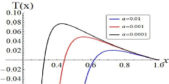
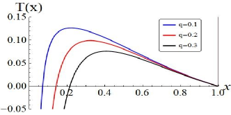
Figure 1: (color online).(a): The radiation temperature $T$ as a function of $x$. The blue line is for $\alpha\mathrm{\ =}0.0001$, whereas the red curve stands for $\alpha\mathrm{\ =}0.01$. Furthermore, the black line is for $\alpha\mathrm{\ =}0.001$. Other parameters are as follows:$r_{c}=1,n=4,q=0.1$. (b): The radiation temperature $T$ as Versus the black hole horizon $x$ with the different values of $q$. The blue line is for $q\mathrm{\ =}0.1$, whereas the red curve stands for $\alpha\mathrm{\ =}0.2$. Furthermore, the black line is for $\alpha\mathrm{\ =}0.3$. Other parameters are as follows:$r_{c}=1,n=4,\alpha=0.0001$.

In Fig. 1(a), we plot the radiation temperature $T$ as the function of positions of the black hole horizon $x$ with the different values of $\alpha$. As shown in the figure, one can see that the maximal value of the two horizon radiation temperature is proportional to $\alpha$, and the region where the temperature is greater than zero is also proportional to the value of $\alpha$ . In Fig.1 (b), we also plot the radiation temperature $T$ as the function of positions of the black hole horizon $x$ with the different values of $q$, we find that the maximal value of the two horizon radiation temperature is proportional to $q$ when choose the same values of $\alpha$, and the region where the temperature is greater than zero is also proportional to the value of $q$.

III Space-time entropy and the effective thermodynamic quantities

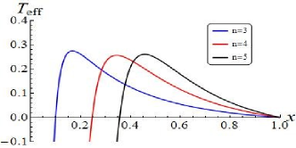
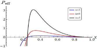
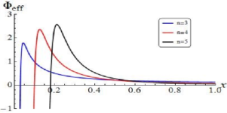
Figure 2: (color online).(a): The effective temperature $T_{eff}$ versus $x$ for the different values of spacetime dimension $n$ : $n=3$ (blue line), $n=4$ (red line),$n=5$ (black line). (b): The effective pressure $p_{eff}$ versus $x$ for the different values of spacetime dimension $n$ : $n=3$ (blue line), $n=4$ (red line),$n=5$ (black line). (c): The effective electric potential $\Phi_{eff}$ versus $x$ for the different values of spacetime dimension $n$ : $n=3$ (blue line), $n=4$ (red line),$n=5$ (black line). Here, $q=0.1,\alpha=0.0001$.

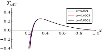
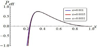
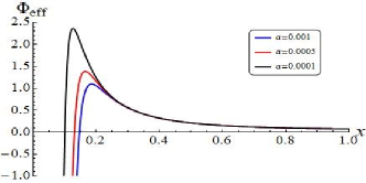
Figure 3: (color online).(a): The effective temperature $T_{eff}$ versus $x$ with different nonlinearity parameter $\alpha$ : $\alpha=0.001$ (blue line), $\alpha=0.0005$ (red line),$alpha=0.0001$ (black line). (b): The effective pressure $p_{eff}$ versus $x$ with different nonlinearity parameter $\alpha$ : $\alpha=0.001$ (blue line), $\alpha=0.0005$ (red line),$alpha=0.0001$ (black line). (c): The effective electric potential $\Phi_{eff}$ versus $x$ with different nonlinearity parameter $\alpha$ : $\alpha=0.001$ (blue line), $\alpha=0.0005$ (red line), $\alpha=0.0001$ (black line). Here, $q=0.1,n=4$.

The first law of thermodynamics is to study the universal relations of the thermal properties. The state parameters of HDBRN space-time satisfies with the first thermodynamic relation formula is written as 49 ; 50

$$dM={T_{eff}}dS-{P_{eff}}dV+{\Phi_{eff}}dQ,$$ (20)

where the effective temperature $T_{eff}$, effective electric potential $\Phi_{eff}$ and the effective pressure $P_{eff}$ are denoted as

$${T_{eff}}={\left({\frac{{\partial M}}{{\partial S}}}\right)_{q,V}}=\frac{{{{\left({\frac{{\partial M}}{{\partial x}}}\right)}_{{r_{c}}}}{{\left({\frac{{\partial V}}{{\partial{r_{c}}}}}\right)}_{x}}-{{\left({\frac{{\partial V}}{{\partial x}}}\right)}_{{r_{c}}}}{{\left({\frac{{\partial M}}{{\partial{r_{c}}}}}\right)}_{x}}}}{{{{\left({\frac{{\partial S}}{{\partial x}}}\right)}_{{r_{c}}}}{{\left({\frac{{\partial V}}{{\partial{r_{c}}}}}\right)}_{x}}-{{\left({\frac{{\partial V}}{{\partial x}}}\right)}_{{r_{c}}}}{{\left({\frac{{\partial S}}{{\partial{r_{c}}}}}\right)}_{x}}}},$$ (21)

$${\Phi_{eff}}={\left({\frac{{\partial M}}{{\partial Q}}}\right)_{S,V}},$$ (22)

$${P_{eff}}=-{\left({\frac{{\partial M}}{{\partial V}}}\right)_{q,S}}=-\frac{{{{\left({\frac{{\partial M}}{{\partial x}}}\right)}_{{r_{c}}}}{{\left({\frac{{\partial S}}{{\partial{r_{c}}}}}\right)}_{x}}-{{\left({\frac{{\partial S}}{{\partial x}}}\right)}_{{r_{c}}}}{{\left({\frac{{\partial M}}{{\partial{r_{c}}}}}\right)}_{x}}}}{{{{\left({\frac{{\partial V}}{{\partial x}}}\right)}_{{r_{c}}}}{{\left({\frac{{\partial S}}{{\partial{r_{c}}}}}\right)}_{x}}-{{\left({\frac{{\partial S}}{{\partial x}}}\right)}_{{r_{c}}}}{{\left({\frac{{\partial V}}{{\partial{r_{c}}}}}\right)}_{x}}}}.$$ (23)

Here, the thermodynamic volume is that between the black hole horizon and the cosmological horizon, namely 27

$$V={V_{c}}-{V_{+}}=\frac{{{V_{n-1}}r_{c}^{n}}}{n}\left({1-{x^{n}}}\right).$$ (24)

Considering the dimension, we assume the space time entropy is

$$S=\frac{{{V_{n-1}}r_{c}^{n-1}}}{4}{F_{n}}(x),$$ (25)

where ${F_{n}}(x)$ is an arbitrary function of $x$.

Substituting Eq. (11), Eq. (24) and Eq. (25) into Eq. (21), one can obtain

$${T_{eff}}=\frac{{(n-1)B(x,q)}}{{4\pi{r_{c}}(1-{x^{n}})A(x)}},$$ (26)

where

$$A(x) = {F_{n}}^{\prime}(x)\left({1-{x^{n}}}\right)+(n-1){F_{n}}(x),{F_{n}}(x)=1+{x^{n-1}}+{f_{n}}(x),$$

$$B(x,q) = k{x^{n-3}}\left({(n-2-n{x^{2}})(1-{x^{n}})+2(n-1){x^{n}}(1-{x^{2}})}\right)$$

$$+\frac{{2{q^{2}}}}{{(n-1)(n-2)r_{c}^{2(n-2)}{x^{n-1}}}}\left({n{x^{n}}(1-{x^{n-2}})-(n-2)(1-{x^{3n-2}})}\right)$$

$$+\frac{{4{q^{4}}\alpha}}{{(3{n^{2}}-7n+4)r_{c}^{4n-6}{x^{3n-3}}}}\left({{x^{n}}(3n-4)(1-{x^{4n-4}})-(4n-4){x^{n}}+n{x^{4n-4}}+(3n-4)}\right).$$

When we set $T_{+}=T_{c}$ , the effective temperature of the spacetime also has the same value

$${T_{c}}={T_{+}}=T={T_{eff}}=\frac{{\tilde{B}(x,q)}}{{4\pi{r_{c}}(1-{x^{n}})A(x)}}.$$ (28)

We can set $\frac{{2{q^{2}}}}{{r_{c}^{2n-4}}}$ as a function of $\frac{{4{q^{4}}\alpha}}{{r_{c}^{4n-6}}}$ and $k$ , then substitute Eq. (13) into Eq. (III), one obtains

$$\frac{{\tilde{B}(x,q)K(x,n)}}{{2{x^{n-2}}(1+{x^{n+1}})}} = k(n-2)(n-1)[n{x^{n-2}}(1-{x^{2}})(1-{x^{n-2}})-(1-{x^{n}})(1-{x^{2n-4}})]$$ (29)

$$+\frac{{(1-{x^{2n-2}})}}{{(3{n^{2}}-7n+4){x^{3n-4}}}}\frac{{4{q^{4}}\alpha}}{{r_{c}^{4n-6}}}[4{x^{n-2}}(1-{x^{n}})+n(1-11{x^{n-2}}+11{x^{2n-2}}-{x^{3n-4}})$$

$$-2{n^{2}}(1-{x^{3n-4}}+5{x^{2n-2}}-5{x^{n-2}})+{n^{3}}(1-{x^{3n-4}}-3{x^{n-2}}+3{x^{2n-2}})].$$

Substituting Eq. (15)and Eq. (29) into Eq. (28),

$$A(x)=\frac{{(n-1){x^{n-2}}(1+{x^{n+1}})}}{{(1-{x^{n}})}}.$$ (30)

When $\frac{{4{q^{4}}\alpha}}{{r_{c}^{4n-6}}}$ as a function of $\frac{{2{q^{2}}}}{{r_{c}^{2n-4}}}$ and $k$ , then substitute Eq. (13) into Eq. (III), we can get

$$\frac{{\tilde{B}(x,q)\tilde{K}(x,n)(3{n^{2}}-7n+4)}}{{2{x^{n-2}}(1+{x^{n+1}})}}$$

$$= k(n-1)(n-2)\left[{4(1-{x^{n}})(1-{x^{4n-6}})}\right.+n[-7(1+{x^{5n-6}})-3{x^{n-2}}(1+{x^{3n-2}})+10{x^{n}}(1+{x^{3n-6}})]$$

$$+{n^{2}}[5{x^{n-2}}(1+{x^{3n-2}})-8{x^{n}}(1+{x^{3n-6}})+3(1+{x^{5n-6}})]+2{n^{3}}[{x^{n}}(1+{x^{3n-6}})\left.{-{x^{n-2}}(1+{x^{3n-2}})]}\right]$$

$$-\frac{{2{q^{2}}(1-{x^{2n-2}})}}{{r_{c}^{2n-4}{x^{n-2}}}}\left[{4{x^{n-2}}(1-{x^{n}})}\right.+n(1-11{x^{n-2}}+11{x^{2n-2}}-{x^{3n-4}})$$

$$-2{n^{2}}(1-{x^{3n-4}}+5{x^{2n-2}}-5{x^{n-2}})+{n^{3}}\left.{(1-{x^{3n-4}}-3{x^{n-2}}+3{x^{2n-2}})}\right].$$

Substituting Eq. (18) and Eq. (III) into Eq. (28), we have

$$A(x)=\frac{{(n-1){x^{n-2}}(1+{x^{n+1}})}}{{(1-{x^{n}})}}.$$ (32)

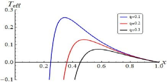
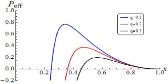
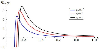
Figure 4: (color online).(a): The effective temperature $T_{eff}$ versus $x$ with the different values of $q$ : $q=0.1$ (blue line), $q=0.2$ (red line),$q=0.3$ (black line). (b): The effective pressure $p_{eff}$ versus $x$ with the different values of $q$ : $q=0.1$ (blue line), $q=0.2$ (red line),$q=0.3$ (black line). (c): The effective electric potential $\Phi_{eff}$ versus $x$ with the different values of $q$ : $q=0.1$ (blue line), $q=0.2$ (red line),$q=0.3$ (black line). Here, $\alpha=0.0001,n=4$.

From Eq. (30) and Eq. (32), one can find that the system entropy satisfied the solution of the differential equation is independent of the selected variables. The solution of Eq. (32) can be written as

$${F_{n}}(x) = \frac{{3n-1}}{{2n-1}}{(1-{x^{n}})^{(n-1)/n}}-\frac{{n(1+{x^{2n-1}})-(2n-1){x^{n-1}}(1+x)}}{{(2n-1)(1-{x^{n}})}}$$ (33)

$$= \frac{{3n-1}}{{2n-1}}{(1-{x^{n}})^{(n-1)/n}}-\frac{{n(1+{x^{2n-1}})+(2n-1)(1-2{x^{n}}-{x^{2n-1}})}}{{(2n-1)(1-{x^{n}})}}+1+{x^{n-1}}$$

$$= {f_{n}}(x)+1+{x^{n-1}.}$$

The case of calculating the Eq (32) is permitted for ${F_{n}}(0)=1$ or ${f_{n}}(0)=0$. It is based on that $x\rightarrow 0$, ${r_{+}}<<{r_{c}}$, which means the spacetime verge to the pure de Sitter spacetime.

From Eq. (30) and Eq. (26), one can obtain the effective temperature

$${T_{eff}}=\frac{{B(x,q)}}{{4\pi{r_{c}}{x^{n-2}}(1+{x^{n+1}})}}.$$ (34)

The effective pressure is

$${P_{eff}}=\frac{{{{(n-1)}^{2}}g(x,q)}}{{4\pi r_{c}^{2}(1-{x^{n}})A(x)}}=\frac{{(n-1)g(x,q)}}{{4\pi r_{c}^{2}{x^{n-2}}(1+{x^{n+1}})}},$$ (35)

with

$$g(x,n) = k\left({\frac{{{x^{n-3}}(1+{x^{n-1}})(n-2+2{x^{n}}-n{x^{2}})}}{{(1-{x^{n}})}}-{x^{n-2}}(n-2)({x^{n-2}}-{x^{n}})}\right)-\frac{{4{q^{4}}\alpha}}{{(3{n^{2}}-7n+4)r_{c}^{2(2n-3)}}}$$

$$\left({\frac{{(1+{x^{n-1}})}}{{1-{x^{n}}}}\frac{{(4n-4){x^{n}}-n{x^{4n-4}}-(3n-4)}}{{{x^{3n-3}}}}-\frac{{(3n-4)(1-{x^{4n-4}})}}{{{x^{2n-2}}}}}\right)$$

$$+\frac{{2{q^{2}}}}{{(n-1)(n-2)r_{c}^{2(n-2)}}}\left({\frac{{(1+{x^{n-1}})}}{{1-{x^{n}}}}\frac{{(2n-2){x^{n}}-n{x^{2n-2}}-(n-2)}}{{{x^{n-1}}}}+(n-2)(1-{x^{2n-2}})}\right).$$

The effective electric potential is

$${\Phi_{eff}} = {\left({\frac{{\partial M}}{{\partial Q}}}\right)_{S,V}}$$ (37)

$$= \frac{{(n-1)(1-{x^{2n-2}})q}}{{(1-{x^{n}})r_{c}^{n-2}{x^{n-2}}}}\left[{\frac{1}{{(n-1)(n-2)}}-\frac{{4{q^{2}}\alpha}}{{(3{n^{2}}-7n+4)r_{c}^{2n-2}}}\frac{{(1+{x^{2n-2}})}}{{{x^{2n-2}}}}}\right].$$

From Eq. (34), Eq. (35) and Eq. (37), we can plot the ${T_{eff}}-x,{P_{eff}}-x,{\Phi_{eff}}-x$ curves for the different values of $n$ in the Fig. 2, respectively. From Fig. 2(a), one can observe that the region of spacetime effective temperature $T_{eff}$ greater than zero is inversely proportional to the number of space-time dimensions. We can also find the maximal value of effective pressure $P_{eff}$is proportional to the number of space-time dimensions when the value of q and $\alpha$ is fixed, as shown in Fig. 2(b). In addition, Fig. 2(c) indicates that the maximal value of effective electric potential $\phi_{eff}$ is also proportional to the number of space-time dimensions when the value of $q$ and $\alpha$ is fixed.

Considering Eq. (34), Eq. (35) and Eq. (37), we can also plot Fig. 3. This figure show the how the effective temperature, pressure and electric potential versus $x$ with the different values of $\alpha$. As shown in Fig. 3(a) and Fig. 3(b), when the values of $n$ and $q$ are fixed, the effective temperature $T_{eff}$ and the effective pressure $P_{eff}$ is not effected by $\alpha$. From Fig. 3(c), one can find that the maximal value of effective electric potential $\Phi_{eff}$ is in direct proportion to the value of $\alpha$.

In addition, as the same method above mentioned, we also plot the curves about ${T_{eff}}-x,{P_{eff}}-x,{\Phi_{eff}}-x$ with the different values of $q$. The Fig.4 indicates that the maximal values of effective temperature $T_{eff}$ and the effective pressure $p_{eff}$ are inversely proportional to the value of is inversely direct proportion to the values of $q$ , while the electric potential is in direct proportion to it.

IV conclusion and discussion

People usually think that black hole thermodynamics is one of the key points to connect gravity and quantum mechanics, and very useful for the study of quantum gravity theory. There are systematic approaches and rich features for the research of black hole thermodynamics in AdS space, especially the criticality, while it’s useless for the research of de Sitter spacetime. The main reason is there are black hole and the cosmological horizons which have different radiation temperature in general, so the spacetime does not satisfy the requirement of stability of thermodynamic equilibrium. Secondly the corresponding thermodynamic systems of two horizons are not independent, there are some relations between them. Therefore, it is important to find a thermodynamic system to describe the de Sitter spacetime completely. The recent references 49 ; 50 proposed a new approach to study the thermodynamics of dS black holes. We use this approach to the higher-dimensional de Sitter spacetime with nonlinear electric field and try to provide the theoretical basis to find the general entropy of the dS black holes and the effective thermodynamical quantities.

From the discussion in Sect. 3, it is known that to find the entropy of the dS black holes and the effective thermodynamical quantities, we need to consider the first law of thermodynamics and the dimension, thus we have equation (25). When the radiation temperature of black hole horizon $T_{+}$ equals the radiation temperature of the cosmological horizon $T_{c}$, i.e. $T={T_{+}}={T_{c}}$, then the effective temperature ${T_{eff}}$ should be same with these two temperature of horizons, i.e. $T={T_{eff}}$. We obtain the differential equation of spacetime entropy, see Eq. 32). And from Eq. (30) and Eq. (32), we know that the differential equation has no relation with the independently parameters we choose. This is same with the research in multi-variables general thermodynamics. It means that the conclusions from HDBRN spacetime thermodynamics are self-consistent. When $x\rightarrow 0$, the spacetime approaches to pure de Sitter as a initial condition and solve the differential equation (30) or (32), then we get the formula of entropy function (33). This formula implies that the entropy of HDBRN spacetime does not include the nonlinear parameters $\alpha$ and $q$, and it is just the function of the position of spacetime horizon. This is consistent with the entropy of black hole horizon $S_{+}$ and the entropy of the cosmological horizon $S_{c}$. What’s more, the effective temperature of HDBRN spacetime given by Eq. (34) is the function of spacetime dimension, the position of horizon and the charge of spacetime $q$ and $\alpha$, the curves of ${T_{eff}}-x$ reflects the relations between various parameters. The effective temperature $T_{eff}$ and the pressure $P_{eff}$ of spacetime are independent of the value of $\alpha$ , The maximum value of the space-time effective potential $\Phi_{eff}$ is proportional to $\alpha$ .This may provide the theoretial foundation for the further research of the classical and quantum features of de Sitter, and its evolution.

References

• (1) D. Kubiznak, R. B. Mann, P-V criticality of charged AdS black holes P-V criticality of charged AdS black holes, JHEP 1207: 033 (2012).
• (2) R. A. Hennigar, E. Tjoa, R. B. Mann, Thermodynamics of hairy black holes in Lovelock gravity, arXiv:1612.06852 [hep-th]
• (3) A. Rajagopal, D. Kubiznak, R. B. Mann, Van der Waals black hole, Phys. Lett. B, 737, 277 (2014).
• (4) S. H. Hendi, R. B. Mann, S. Panahiyan, B. Eslam Panah, van der Waals like behavior of topological AdS black holes in massive gravity, Phys. Rev. D 95, 021501(R) (2017).
• (5) R. G. Cai, L. M. Cao, L. Li, and R. Q. Yang, P-V criticality in the extended phase space of Gauss-Bonnet black holes in AdS space, JHEP,(9), 1-22 (2013).
• (6) R.G. Cai, S. M. Ruan, S. J. Wang, R. Q. Yang, R. H. Peng, Complexity Growth for AdS Black Holes, JHEP 1609,161 (2016).
• (7) J. L. Zhang, R. G. Cai, H. W. Yu, Phase transition and Thermodynamical geometry of Reissner-Nordström-AdS Black Holes in Extended Phase Space, Phys. Rev. D 91, 044028 (2015).
• (8) J. L. Zhang, R. G. Cai, H. W. Yu, Phase transition and thermodynamical geometry for Schwarzschild AdS black hole in AdS5$\times$S5 spacetime, JHEP, 02, 143 (2015).
• (9) S. H. Hendi, B. Eslam Panah, S. Panahiyan, Massive charged BTZ black holes in asymptotically (a)dS spacetimes, JHEP 05, 029 (2016).
• (10) W. Xu, H. Xu, L. Zhao, Gauss-Bonnet coupling constant as a free thermodynamical variable and the associated criticality, Eur. Phys. J. C 74: 2970 (2014).
• (11) S. W. Wen, Y. X. Liu, Triple points and phase diagrams in the extended phase space of charged Gauss-Bonnet black holes in AdS space, Phys. Rev. D90, 044057 (2014).
• (12) W. G. Brenna, R. B. Mann, M. Park, Mass and Thermodynamic Volume in Lifshitz Spacetimes, Phys. Rev. D 92, 044015 (2015).
• (13) Z. Dayyani, A. Sheykhi, and M. H. Dehghani, Counterterm method in Einstein dilaton gravity and the critical behavior of dilaton black hole with a power-Maxwell field. Phys. Rev. D 95, 84004 (2017).
• (14) M. K. Zangeneh, A. Dehyadegari, A. Sheykhi, M. H. Dehghani, Thermodynamics and gauge/gravity duality for Lifshitz black holes in the presence of exponential electrodynamics, JHEP 1603, 037 (2016).
• (15) M. H. Dehghani, A. Sheykhi, S. E. Sadati, Thermodynamics of nonlinear charged Lifshitz black branes with hyperscaling violation, Phys. Rev. D 91, 124073 (2015).
• (16) R. Banerjee, B. R. Majhi, S. Samanta, Thermogeometric phase transition in a unified framework, Phys. Lett. B 767, 25 - 28 (2017).
• (17) R. Banerjee, Di. Roychowdhury, Thermodynamics of phase transition in higher dimensional AdS black holes, JHEP 11,004 (2011).
• (18) R. Banerjee, D. Roychowdhury, Critical behavior of Born Infeld AdS black holes in higher dimensions, Phys. Rev. D 85, 104043 (2012).
• (19) M. S. Ma, R. Zhao, Y. S. Liu, Phase transition and thermodynamic stability of topological black holes in Hořava-Lifshitz gravity, Classical and Quantum Gravity, 34, 165009 (2017).
• (20) M. S. Ma, R. H. Wang, Peculiar P-V criticality of topological Hořava-Lifshitz black holes, Phys. Rev. D 96, 024052 (2017).
• (21) S. H. Hendi, B. Eslam Panah, S. Panahiyan, M. S. Talezadeh, Geometrical thermodynamics and P-V criticality of the black holes with power-law Maxwell field, Eur. Phys. J. C 77, 133 (2017).
• (22) D. C. Zou, Y. Q. Liu, R. H. Yue, Behavior of quasinormal modes and Van der Waals-like phase transition of charged AdS black holes in massive gravity, Eur. Phys. J. C 77, 365 (2017).
• (23) P. Cheng, S. W. Wei, Y. X. Liu, Critical phenomena in the extended phase space of Kerr-Newman-AdS black holes, Phys. Rev. D 94, 024025 (2016).
• (24) M. Mir, R. B. Mann, Charged Rotating AdS Black Holes with Chern-Simons coupling, Phys. Rev. D 95, 024005 (2017).
• (25) Z. X. Zhao, J. L. Jing, Ehrenfest scheme for complex thermodynamic systems in full phase space. JHEP 11 (2014) 037.
• (26) R. Zhao, H. H. Zhao, M. S. Ma, L. C. Zhang, the critical phenomena and thermodynamics of charged topological dilaton AdS black holes,Eur. Phys. J. C 73, 2645 (2013).
• (27) B. P. Dolan, D. Kastor, D. Kubiznak, R. B. Mann, Jennie Traschen, Thermodynamic Volumes and Isoperimetric Inequalities for de Sitter Black Holes, Phys. Rev. D 87, 104017 (2013).
• (28) Y. Sekiwa, Thermodynamics of de Sitter black holes: Thermal cosmological constant. Phys. Rev. D 73, 084009 (2006).
• (29) R. Bousso and S. W. Hawking, Pair creation of black holes during inflation Phys. Rev. D 54, 6312 (1996).
• (30) R. Bousso and S. W. Hawking, (Anti-)evaporation of Schwarzschild?de Sitter black holes, Phys. Rev. D 57, 2436 (1998).
• (31) I. Arraut, The Astrophysical Scales Set by the Cosmological Constant, Black-Hole Thermodynamics and Non-Linear Massive Gravity, Universe, 3, 45 (2017).
• (32) I. Arraut, D. Batic, M. Nowakowski, Comparing two approaches to Hawking radiation of Schwarzschild-de Sitter Black Holes. Class. Quantum Gravity 26, 125006 (2009).
• (33) I. Arraut, The Planck scale as a duality of the Cosmological Constant: S-dS and S-AdS thermodynamics from a single expression, arXiv:1205.6905v3.
• (34) M. Urano and A. Tomimatsu, Mechanical First Law of Black Hole Spacetimes with Cosmological Constant and Its Application to Schwarzschild-de Sitter Spacetime. Class. Quant. Grav. 26, 105010 (2009).
• (35) F. Mellor, and I. Moss, Black holes and gravitational instantons, Class. Quant. Grav. 6, 1379 (1989).
• (36) F. Mellor, and I. Moss, Black holes and quantum wormholes, Phys. Lett. B 222, 361(1989).
• (37) W. Xu, J. Wang, X. H. Meng, Entropy relations and the application of black holes with cosmological constant and Gauss-Bonnet term, Physics Letters B 742, 225-230 (2015).
• (38) S. H. Hendi, A. Dehghani, Mir Faizal, Black hole thermodynamics in Lovelock gravity’s rainbow with (A)dS asymptote, Nucl. Phys. B 914, 117 (2017).
• (39) D. Kubiznak, F. Simovic, Thermodynamics of horizons: de Sitter black holes and reentrant phase transitions. Class. Quant. Grav. 33, 245001 (2016).
• (40) J. McInerney, G. Satishchandran, J. Traschen, Cosmography of KNdS Black Holes and Isentropic Phase Transitions, Class. Quant. Grav. 33, 105007 (2016).
• (41) Sourav Bhattacharya, Amitabha Lahiri, Mass function and particle creation in Schwarzschild-de Sitter spacetime, Eur. Phys. J. C 73, 2673 (2013).
• (42) M. Azreg-Aïnou, Black hole thermodynamics: No inconsistency via the inclusion of the missing P-V terms, Phys. Rev. D 91, 064049 (2015). M. Azreg-Aïnou, Charged de Sitter-like black holes: quintessence-dependent enthalpy and new extreme solutions, arXiv:1410.1737 [gr-qc].
• (43) P. Kanti and T. Pappas, Effective Temperatures and Radiation Spectra for a Higher-Dimensional Schwarzschild-de-Sitter Black-Hole, Phys. Rev. D 96, 024038 (2017).
• (44) J. D. Bekenstein, Extraction of energy and charge from a black hole, Phys. Rev. D 7, 949 (1973).
• (45) J. M. Bardeen, B. Carter, and S. W. Hawking, The four laws of black hole mechanics, Commun. Math. Phys. 31, 161 (1973).
• (46) S. W. Hawking, Black hole explosions? Nature 248, 30 (1974).
• (47) S. Hawking and D. N. Page, Thermodynamics of black holes in anti-de Sitter space, Commun. Math. Phys. 87, 577 (1983).
• (48) G. Gibbons, R. Kallosh, and B. Kol, scalar charges and the first law of black hole thermodynamics, Phys. Rev. Lett. 77, 4992 (1996).
• (49) S. H. Hendi, and M. Momennia,Thermodynamic instability of topological black holes with nonlinear source, Eur. Phys. J. C 75, 54 (2015).
• (50) Wald R M. Asymptotic behavior of homogeneous cosmological models in the presence of a positive cosmological constant[J]. Physical Review D, 28, 2118 (1983).
• (51) Peebles P J E, Ratra B. Cosmology with a time-variable cosmological’constant’. The Astrophysical Journal, 325, 17-20 (1988).
• (52) S. H. Hendi and R. Naderi, Geometrothermodynamics of black holes in Lovelock gravity with a nonlinear electrodynamics, Phys. Rev. D 91, 024007 (2015).
• (53) R. G. Cai, J. Y. Ji and K. S. Soh, Action and entropy of black holes in spacetimes with a cosmological constant, Class. Quantum Grav. 15, 2783?2793 (1998).
• (54) L. C. Zhang, R. Zhao, M. S. Ma, Entropy of Reissner–Nordström–de Sitter black hole. Physics Letters B 761, 74–76 (2016).
• (55) H. F. Li, M. S. Ma, L. C. Zhang, R. Zhao, Entropy of Kerr–de Sitter black hole. Nucl. Phys B 920, 211–220 (2017).