The magnon-mediated attraction between two holes doped in a CuO₂ layer

Abstract

Using a realistic multi-band model for two holes doped into a CuO₂ layer, we devise a method to turn off the magnon-mediated interaction between the holes. This allows us to verify that this interaction is attractive, and therefore could indeed be (part of) the superconducting glue. We derive its analytical expression and show that it consists of a novel kind of pair-hopping+spin-exchange terms. Its coupling constant is fitted from the ground state energy obtained with variational exact diagonalization, and it faithfully reproduces the effect of the magnon-mediated attraction in the entire Brillouin zone. For realistic parameter values, this effective interaction is borderline strong enough to bind the holes into preformed pairs.

I Introduction

Despite sustained efforts, more than thirty years after the discovery of high-temperature superconductivity in cuprates,Bednorz and Müller (1986) the nature of the glue that binds its Cooper pairs is still unclear. Anderson (2007) This binding is not through the phonon-mediated Bardeen-Cooper-Schrieffer (BCS) mechanism responsible for low-T_c, conventional superconductivity,Bardeen, Cooper and Schrieffer (1957) although phonons have been proposed as the glue for bipolaron superconductivity. Alexandrov and Mott (1994); Alexandrov (2009); Kresin and Wolf (2009) The current leading contender appears to be a magnon glue Moriya and Ueda (2000); Lee et al. (2006); Ogata and Fukuyama (2008); Monthoux et al. (2007); Val’kov and Barabanov (2016) due to the proximity of antiferromagnetism in the phase diagram of these strongly correlated materials, and also because of the existence of several other non-conventional superconductors with an adjacent magnetically-ordered phase.Dai (2015); Stewart (1984) Other, more exotic proposed glues include loop currents,Varma (2006) orbital relaxation Hirsch (2014) or hidden fermions.Sakai et al. (2016) A mix of several glues is certainly also possible. Cataudella et al. (2007); Dal Conte et al. (2012)

Part of the reason for the absence of a definitive theoretical answer is the fact that most such work is based on effective models or on phenomenological considerations, with parameters extracted from fits of various experimental measurements. Such approaches are a priori guaranteed to reproduce some experimental aspects, but it is not clear if the values of the fitted parameters are reasonable, nor how they should depend on the microscopic structure or on external parameters such as pressure, doping, etc. Such theories are hard to falsify.

What is needed, instead, is to extract the form and the strength of the effective attraction mediated by various glues, starting from well-established microscopic models. In a second stage, these effective interactions should then be investigated to see if they can explain the high-T_C superconductivity (and hopefully many other aspects of the complex cuprate phenomenology) on their own, or if combinations of several such terms are necessary. Clearly, this would make the process of validating or falsifying various mechanisms more straightforward. The problem, however, is that extracting these effective attractions from microscopic models is very difficult, for two reasons: (i) perturbative methods are unsuitable whether one believes the cuprates to be strongly-correlated electron systems, and/or to have the strong electron-phonon coupling that could enable a high T_C value. Moreover, one cannot appeal (only) to numerical methods to obtain the needed analytical expressions for these effective attractions. Instead, accurate (semi)analytical formalisms are needed, and those are hard to come by; (ii) more fundamental is a problem stemming from the indistinguishability of electrons. The effective interactions arise from processes where one particle emits a boson, which is then absorbed by another particle. If one could turn off this process “by hand” and thus compare results where this exchange is allowed vs. forbidden, one could infer the form and magnitude of this effective boson-mediated interaction from its effects on the many-body spectrum and wavefunctions. The problem is that for indistinguishable particles it is impossible to tell which is “particle 1” and which is “particle 2”, in other words to distinguish whether a boson has been exchanged or whether it has been re-absorbed by the same particle that emitted it (thereby contributing to renormalizing it into a quasiparticle, instead of to the boson-mediated interaction).

In this work we propose an elegant solution for these challenges that allows us to verify that magnon-exchange indeed mediates an effective attraction between two holes doped into a cuprate layer. Moreover, we find the analytical expression of this effective attraction. Our expression describes processes that are conceptually simple, namely pair-hopping+exchange terms where both holes hop while also exchanging their spins. To the best of our knowledge, this type of effective interaction has not been considered before in this context. We extract its energy scale by fitting the ground-state energy, specifically we ask that the ground-state energy of the system with magnon-exchange allowed is reproduced by that of the system where the magnon-exchange is turned off, but this additional effective attraction is added instead. We then show that our effective interaction reproduces well the effects of the magnon-exchange throughout the Brillouin zone, thus validating its expression and magnitude.

The paper is organized as follows. Section II presents the model and describes its two-hole spectrum. Section III discusses how we prove the existence of a magnon-mediated attraction between the holes, and how we quantify its form and magnitude. Section IV analyzes the role of the background spin fluctuations, while Section V speculates on the possible existence of pre-formed pairs. Finally, Section VI contains a short summary and conclusions. Various technical details are relegated to the three Appendixes.

II The model and its two-hole spectrum

It is well-known that in the doped cuprates, the doped holes reside in the O $2p$ band, thus a reasonable starting point for an accurate description is the three-band Emery model Emery (1987); mod which includes both the Cu $3d_{x^{2}-y^{2}}$ orbitals that host the strongly-correlated holes responsible for the long-range antiferromagnetic (AFM) order in the parent compounds, but also the ligand O $2p$ orbitals hosting the additional doped holes responsible for superconductivity.

We study the $U_{dd}\rightarrow\infty$ limit of the three-band Emery model. This is justified physically because $U_{dd}$ is by far the largest energy scale, and is necessary computationally to make the Hilbert space manageable. The $U_{dd}\rightarrow\infty$ limit implies that single-hole occupancy is enforced for the Cu $3d_{x^{2}-y^{2}}$ orbitals, so there are spins-${1\over 2}$ at these sites. Additional (doped) holes occupy states in the O-$2p$ band derived from the ligand $2p$ orbitals, as sketched on the right-hand side of Fig. 1(a).

We believe this to be a more suitable starting point than the more studied one-band $t-J$ and Hubbard models because the one-band models make the additional assumption that the doped holes are locked into Zhang-Rice singlets (ZRS) Zhang and Rice (1988); Eskes and Sawatzky (1988) and perform a further projection onto those states. Even if the ZRS provides a good description of a single quasiparticle (qp), it would not necessarily follow that modeling the many-hole system in terms of ZRS is valid. Nearby holes may modify the magnetic background and exchange magnons in a way not allowed if each hole is locked in a ZRS.Moeller et al. (2012a) Our approach has fewer constraints as it does not impose the formation of ZRS, although it allows it to occur if it turns out to be the most energetically favorable option. By being more general, our model allows for, and tests, more possible scenarios.

Moreover, in previous work Ebrahimnejad et al. (2014, 2016) we showed a qualitative difference between the quasiparticle (qp) of our model and that of the optimized $t$-$t^{\prime}$-$t^{\prime\prime}$-$J$ model: while both models predict a qp in agreement with that measured experimentally, the dispersion in the one-band models is significantly impacted by background spin fluctuations, unlike that of our model. The physical origin of this difference is discussed below in detail. Here we note that its existence suggests that these models do not describe the same physics even in the single qp sector, so there is no reason to expect them to describe the same magnon-mediated exchange in the two-hole sector.

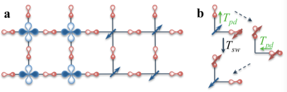
Figure 1: (a) Sketch of three-band model which includes the Cu $3d_{x^{2}-y^{2}}$ and the O ligand $2p_{x/y}$ orbitals (left half). In the strongly-correlated limit, there are spin degrees of freedom at Cu sites while the doped holes move on the O sublattice, as sketched in the right half; (b) A $T_{sw}$ process which results in effective hopping of the hole while its spin is swapped with that of the neighbour Cu.

To obtain the many-hole Hamiltonian, we start from the Emery model and take its $U_{dd}\rightarrow\infty$ limit by straightforward generalization of the method used for one hole in Ref. Lau et al., 2011a. The resulting Hamiltonian is:

$${\cal H}=T_{pp}+U_{pp}+T_{sw}+H_{J_{pd}}+H_{J_{dd}}.$$ (1)

Briefly, $T_{pp}$ includes first and second nearest neighbour (nn) hopping of the doped holes between ligand O $2p$ orbitals, while $U_{pp}$ is the corresponding on-site repulsion. $T_{sw}$ describes effective hopping of doped holes mediated by the Cu spin, whereby the Cu hole hops onto a neighbour O followed by the doped hole filling the Cu orbital, as sketched in Fig. 1(b); this leads to a swap of the spins of the hole and the Cu. $H_{J_{pd}}$ is the AFM exchange between the spins of the doped holes and those of their neighbouring Cu. Finally, $H_{J_{dd}}$ is the nn AFM superexchange between adjacent Cu spins, apart from bonds occupied by holes. Setting $J_{dd}\approx 150$meV as the energy unit, we find $t_{pp}=4.13,t_{pp}^{\prime}=2.40,U_{dd}=25.40,t_{sw}=2.98$ and $J_{pd}=2.83$, respectively. Lau et al. (2011a); Ebrahimnejad et al. (2014, 2016) Note that the value of $t_{sw}$ is changed if a second hole is on either O involved, because $U_{pp}$ shifts the energy of the intermediary states. This is taken into account in our calculations, although we found it to have essentially no consequences. The detailed description of all these terms and several other relevant technical details are given in Appendix A.

In the undoped system, only the AFM superexchange $H_{J_{dd}}$ acts between neighbor Cu spins. This Heisenberg-type exchange results in a very complicated undoped ground-state (GS), which has strong short-range AFM fluctuations but no long-range order. This is unlike the real materials, which acquire long-range AFM order due to coupling to neighboring layers.

To make progress, we begin by simplifying $H_{J_{dd}}$ to an Ising form, so that the undoped ground-state is a Neél state without spin fluctuations. At first sight, it may seem counterintuitive that this is a reasonable approximation (even though it produces a GS with long-range order, much more similar to that of the actual material than is the GS of the Heisenberg model). In fact, this turns out to be an excellent approximation for this model, so far as the behavior of doped holes is concerned, at least in the extremely underdoped limit we study here. Indeed, as shown in Refs. Ebrahimnejad et al., 2014, 2016 for a single doped hole, this approximation is justified because $J_{dd}$ is significantly smaller than all other energy scales. Physically, this means that the time-scale over which the background spin fluctuations occur is significantly longer than that over which the holes move around and modify their local magnetic environment and exchange magnons through the spin-offdiagonal parts of $T_{sw}$ and $H_{J_{pd}}$. Because spin fluctuations are so slow, their influence on these fast processes involving the holes is minor. Below, we verify explicitly that this holds true for the magnon-mediated interaction between the holes, by allowing background spin-fluctuations to occur in the vicinity of the holes. As discussed later, we find that their presence changes the magnitude of the magnon-mediated interactions by only a few percent, so indeed they are negligible. As mentioned, this is in sharp contrast to what happens in one-hole models, where the spin-fluctuations occur on time-scales comparable to those relevant for processes involving the doped holes, so they significantly influence their dispersion (and presumably the effective interations, too).Ebrahimnejad et al. (2016)

In the absence of background spin fluctuations, only the holes emit and absorb magnons of the Cu magnetic background. For the Ising $H_{J_{dd}}$, magnons are static flipped Cu spins. The absence of dispersion as compared to a Heisenberg $H_{J_{dd}}$ may seem problematic, but again it is the small $J_{dd}$ that controls the magnon speed. Because this speed is small compared to that of other relevant processes, it can be safely set to zero: a magnon emitted by a hole is simply too slow to move away before it is absorbed either by the same hole or by a different one. Another way to think about this is that what matters here are real-space configurations, i.e. how far is a magnon from a hole. A local (in space) magnon is a linear superposition of all $\vec{q}$-momentum magnons. For symmetry reasons, the coupling of small-$\vec{q}$ magnons to holes vanishes, so the holes interact mostly with the large-$\vec{q}$ magnons, whose dispersion is rather flat and which, therefore, can be safely treated as being immobile.

If only the holes create and absorb magnons, we can meaningfully classify variational spaces in terms of their magnon numbers: the more magnons, the higher their Ising energy cost, and the less likely to find such configurations contributing significantly to low-energy eigenstates. In this work, we limit the variational space to have up to two magnons, and moreover require that any magnon is within a distance $m_{C}$ from a hole - the reason being that we are interested in the low-energy states where the magnons belong to qp clouds and therefore are never too far from holes. This variational space suffice to allow us to characterize the magnon-exchange between holes, which is our goal. It is also sufficient to quantitatively capture the dispersion of a single quasiparticle. Ebrahimnejad et al. (2014, 2016) For two holes, this space is too limited and overestimates the quasiparticles’ bandwidth, but this aspect can be mitigated (see discussion below). The alternative of increasing the variational space (and thus run times and memory resources) by allowing more magnons is less palatable considering that we are already dealing with up to $10^{6}$ configurations. This is because for two-hole configurations we need a second cutoff $M_{C}$ for the maximum allowed distance between any two objects (holes and/or magnons); to study unbound states properly, this cutoff can run to many tens of lattice constants. More technical details regarding the variational space, as well as the single-qp dispersion, are presented in Appendix B.

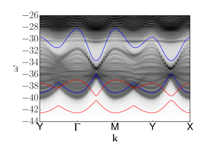
Figure 2: Contour plot of the two-hole spectral function $A(\mathbf{k},\omega)$ along the high symmetry lines of the BZ. This spectral weight is for states where one hole is on the $p_{x}$, and the other is on the $p_{y}$ orbital adjacent to the same Cu. Clearly, the lowest-energy feature in the two-hole spectrum is a continuum. The blue and red lines indicate the expected continuum boundaries obtained from the convolution of single-qp dispersions when $n_{m}=1$ and $n_{m}=2$, respectively, i.e. when each qp is allowed to have up to 1 or up to 2 magnons in its cloud, respectively. The other cutoffs are $M_{c}=40$ and $m_{c}=3$.

Diagonalizing Hamiltonian (1) in this variational space reveals that the lowest feature of the two-hole spectrum is the continuum describing two unbound qps, shown in Fig. 2 as the gray-scale contour plot. To verify this, we use our knowledge of the single qp dispersion $\epsilon_{\mathrm{sp}}(\mathbf{k})$ (shown in Appendix B) to find the expected location of the two-hole continuum. This corresponds to the convolution of two single-qp spectra, and for a total momentum $\mathbf{k}$ it spans $\{\epsilon_{\mathrm{sp}}(\mathbf{k}-\mathbf{q})+\epsilon_{\mathrm{sp}}(\mathbf{q})\}_{\mathbf{q}\in\mathrm{BZ}}$. The blue (top) set of lines show the expected location of the continuum if each qp cloud is constrained to have up to $n_{m}=1$ magnons, while the red (bottom) set of lines is the answer if each qp cloud is constrained to have up to $n_{m}=2$ magnons.

As expected, our answer lies in between the two limits, because in the two-hole variational space that we use, with some probability each qp can have more than one magnon, however the space is not large enough so that both holes can have 2 magnons each at the same time. We verified that if we impose the additional restriction for the two-hole variational space that when 2 magnons are present, each hole has a magnon within $m_{c}$ of it, we recover perfect agreement between the two-hole continuum and the $n_{m}=1$ single-hole prediction (not shown). We can also artificially increase $J_{dd}$ leading to a higher energy cost for magnons and thus less weight on the two-magnon states. For very large $J_{dd}$, the red and blue lines in Fig. 2 fall on top of each other and coincide with the continuum edge of the two-hole calculation (not shown).

We are thus confident that this lowest-energy continuum is indeed the two-qps continuum, which is always a part of the two-hole spectrum. Unfortunately, this result gives no clue about the effective interaction between the qps, as the continuum would be present whether the two qps are non-interacting or whether they experience attraction or repulsion. All we can say is that if there is magnon-mediated attraction between the two qps, it does not appear to be strong enough to bind them into a “pre-formed” pair, which would be a discrete state lying below this two-qp continuum (we revisit this point below). However, from this result we cannot even infer whether there is a magnon-mediated interaction.

To do that, we need to find a way to turn off magnon-exchange processes, in order to gauge their effect on the two-qps eigenstates. We describe how we achieve this goal in the next section.

III Quantifying the effective magnon-mediated interaction

As already mentioned in the Introduction, the key difficulty with turning off magnon-exchange processes is in figuring out when a magnon has actually been exchanged. This can be seen by considering the configurations of the variational space, sketched in Fig. 3(a). The top line indicates configurations with a spin-up and a spin-down hole plus the AFM background (the holes are at various locations but for simplicity we do not label these). Either hole can create a magnon in the appropriate magnetic sublattice; this leads to the one-magnon configurations from the second line. Either hole can emit a second magnon resulting into two-magnon configurations like in the third line. In principle, any number of magnons can be emitted so this hierarchy of configurations is infinite, but as mentioned we keep only up to two-magnon configurations in our variational space.

In the zero- and two-magnon configurations, the holes are distinguishable through their spins (no term in Hamiltonian (1) allows direct hole-hole spin exchange). However, in the one-magnon configurations both holes have identical spin and thus are indistinguishable. This is why when considering the magnon absorption from such a configuration, it is impossible to know which of the two holes flipped its spin to emit the magnon in the first place. As a result, we cannot forbid magnon-exchange processes at this level, as this requires us being able to distinguish between the indistinguishable holes.

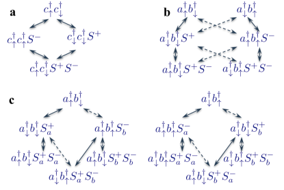
Figure 3: (a) Original variational space, consisting of no-magnon (top line), one-magnon (middle line) and two-magnon (bottom line) configuration. The holes and/or magnons can be at any sites consistent with the cutoffs, but for simplicity we do not label their positions; (b) Variational space when the holes are given flavors $a$ or $b$. This can be mapped exactly onto the original variational space of (a) using antisymmetric combinations of the two flavors; (c) Extended variational space where magnons also have a flavor. This allows us to turn off the exchange of magnons between holes.

We therefore must assign different flavors $a$ and $b$ to the holes, so that they are distinguishable even when they have the same spin. This results in the configurations of Fig. 3b. Interestingly, these two variational spaces map exactly onto each one if we use the correspondence $c^{\dagger}_{\sigma}c^{\dagger}_{\sigma^{\prime}}\leftrightarrow(a^{\dagger}_{\sigma}b^{\dagger}_{\sigma^{\prime}}-a^{\dagger}_{\sigma^{\prime}}b^{\dagger}_{\sigma})/\sqrt{2}$, which is necessary to enforce Pauli’s principle. However, for these antisymmetrized, physical states, it is still impossible to know which particle emitted the magnon, just like for the original states onto which they map. For instance, if the system is in a $a^{\dagger}_{\downarrow}b^{\dagger}_{\downarrow}S^{+}$ type of configuration, it may have arrived there either by starting in the $a^{\dagger}_{\uparrow}b^{\dagger}_{\downarrow}$ sector of the physical state with the $a$-type hole emitting the magnon, or by starting in the $a^{\dagger}_{\downarrow}b^{\dagger}_{\uparrow}$ sector with the $b$-type hole emitting the magnon. The two scenarios cannot be distinguished, therefore we still cannot know which hole emitted the magnon so we cannot decide if a magnon-absorption process is of magnon-exchange type or of quasiparticle renormalization type.

This is why we need to also label the magnons as $a$ or $b$, according to which hole emitted them. This leads to the variational space sketched in Fig. 3c, which we call the “enlarged variational space”. In this enlarged space we can turn off the magnon-exchange by requiring that an $a/b$ magnon can only be absorbed by an $a/b$ hole. Its states are divided into two families that do not mix if the magnon-exchange is turned off, which is the situation sketched in Fig. 3c. Again, the physical states are the antisymmetrized combinations originating from $(a^{\dagger}_{\sigma}b^{\dagger}_{\sigma^{\prime}}-a^{\dagger}_{\sigma^{\prime}}b^{\dagger}_{\sigma})/\sqrt{2}$ zero-magnon configurations, but now for the situation sketched in Fig. 3c, we know that to arrive at a $a^{\dagger}_{\downarrow}b^{\dagger}_{\downarrow}S^{+}_{a}$ configuration, the $a$-type of hole emitted the magnon. If only the $a$-type hole can absorb it, then magnon-exchange is turned off, and we can contrast the results in its absence to those obtained when magnon-exchange is allowed. From such comparisons we ought to be able to infer the effects of the magnon-exchange, in particular whether they result in an effective attraction between the qps.

Before continuing, we must note that the mapping of the antisymmetrized, physical states from the extended variational space onto their counterparts in the original basis is no longer one-to-one, because of the increased number of one- and two-magnon configurations. Instead, the enlarged variational space can be thought of as corresponding to the tensor product of the variational spaces for single spin-up and spin-down holes, respectively, but with the physical constraints imposed, e.g. two magnons cannot be at the same Cu site, etc. This is meaningful because in the low-energy states, magnons are bound to their hole’s cloud and therefore need not be treated as free particles.

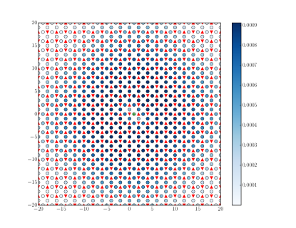
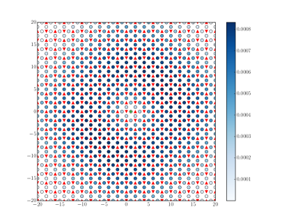
Figure 4: Contour plots (shades of blue) for the GS probability to find a hole on various O sites (shown by circles), if the other other hole is at the central $p_{x}$ O site marked with the green cross. The red arrows are at the positions of Cu and indicate the direction of the spins in the undoped ground state, i.e. before the holes were added. Top panel shows the result when magnon-exchange is allowed, while the bottom panel shows the result when magnon-exchange is turned off.

Figure 4 shows GS results for the case when the magnon-exchange is allowed (top panel) em vs. forbidden (bottom panel). The red arrows are at the positions of Cu sites and indicate the direction of their spins in the undoped ground state. Of course, the spin order is modified by the presence of the holes but showing that in a meaningful way on this scale is impossible, which is why we show the magnetic order before the holes were introduced. The O locations are indicated by circles. Their blue shading indicates the probability to find a hole on that O, if the other hole is located on the central $p_{x}$ orbital marked by the green cross.

Clearly, when the magnon-exchange is allowed, the the holes are closer than when the magnon-exchange is turned off. This clearly proves that magnon-exchange mediates an effective attraction between the two holes. This is one of the main results of this study.

Before trying to quantify how strong is this attraction, we point out two important facts. First, this GS is at the bottom of the two-qps continuum, so these two holes are not bound. The reason why there is finite probability for them to be close to one another is the existence of the constraint $M_{c}$ on the largest relative distance allowed between them. This imposes a “finite-box” type of restriction on the relative motion of the two holes, so they cannot move infinitely far apart. We have checked that the tendency of holes to be closer when magnon-exchange is allowed is independent of the size of the $M_{c}$ cutoff, as indeed expected for an interaction with a finite range. This is shown in Figure 5(a), where we plot the cumulative probability $P(r)={1\over N}\sum_{i}\sum_{|j|<r}\langle GS|\hat{n}_{i}\hat{n}_{i+j}|GS\rangle$ to find the holes within a distance $|j|\leq r$ (measured using the L1-norm) versus the scaled separation $r/M_{C}$, for several values of the maximum allowed relative distance $M_{C}$. Curves with different $M_{C}$ overlap, showing that these are indeed unbound states: the holes move further apart if $M_{C}$ is larger. The full/dashed lines show the results with/without magnon-exchange. In its presence the holes are closer to each other, therefore magnon-exchange mediates an effective attraction between holes.

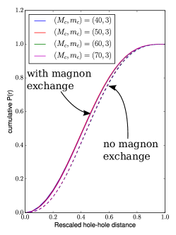
Figure 5: (color online) GS cumulative probability $P(r)$ to find the two holes within a distance $r/M_{c}$ of each other, when magnon-exchange is allowed/forbidden (full/dashed lines). The results are essentially independent of the values of the cutoffs $M_{c},m_{c}$.

The second note is that the GS is doubly degenerate. The contour plots of Fig. 4 will look somewhat different depending on which linear combination of the two eigenstates is chosen for calculating the probability. The choice we made in Fig. 4 is to use the eigenstate that is even to reflections about the $x-y$ diagonal. Irrespective of which choice is made, the holes are always closer to one another when magnon-exchange is allowed.

Next, we identify $H_{\rm{eff}}$ that describes this magnon-mediated attraction. This is achieved by adding various possible candidates for $H_{\rm{eff}}$ to the calculation in the enlarged space without magnon-exchange, and adjusting until the results match those with magnon-exchange allowed. We use perturbation theory (PT) to suggest possible forms: $H_{\rm{eff}}\sim\hat{P}_{0}\hat{V}\frac{1-\hat{P}_{0}}{E_{0}-{\cal H}_{0}}\hat{V}\hat{P}_{0}$, where $\hat{P}_{0}$ projects onto the zero-magnon subspace, ${\cal H}_{0}$ contains terms that conserve the number of magnons and $\hat{V}={\cal H}-{\cal H}_{0}$ contains terms that create or annihilate magnons.

Clearly, ${\hat{V}}$ has contributions from $T_{sw}$ and $H_{J_{pd}}$. These are further divided into direct processes where holes create/remove magnons of their own flavor, vs. exchange ones, where they interact with magnons of the other flavor (only direct processes are allowed when the magnon-exchange is turned off). To mimic the effect of the magnon-exchange, $H_{\rm{eff}}$ must contain the product between a direct and an exchange term – eg. a hole emits a magnon of its own flavor (direct process) which the other hole then absorbs (exchange process).

Generating all such terms suggested by PT and enforcing hermiticity, we find four possible contributions to $H_{\rm{eff}}$ (the details are provided in Appendix C). We then investigate each term separately, treating its magnitude as a free parameter, fitted to get the same GS energy as for the full calculation with magnon-exchange allowed. This approach allows us to account for the renormalization of this energy scale due to higher order terms in the perturbative expansion.

We find that the dominant term has both the magnon emission and absorption due to $T_{\rm{sw}}$. This finding is consistent with the independent check that turning off the magnon-exchange due to this term accounts for nearly all the difference between the cumulative probabilities of Fig. 5 (not shown).

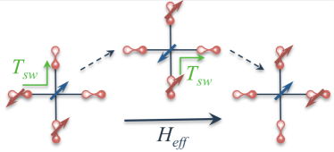
Figure 6: (color online) Sketch of one of the terms in $H_{\rm eff}$. Both holes hop through $T_{\rm{sw}}$ processes, exchanging a magnon through the common Cu spin. All possible such processes are included in $H_{\rm eff}$, with the same magnitude but signs depending on $pd$ overlaps.

Keeping only this dominant term, we find $H_{\rm{eff}}=\sum_{j}(H_{\rm{eff}}^{j\uparrow}+H_{\rm{eff}}^{j\downarrow})$ where the two terms correspond to having both holes adjacent to the up/down Cu spin in the unit cell $j$, and:

$$H_{\rm{eff}}^{j\uparrow}=t_{\rm{pair}}\!\!\!\!\!\!\sum_{\alpha,\beta,\eta_{\alpha}\atop\eta_{\beta}\neq u_{\alpha}-u_{\beta}}\!\!\!\!\!\!\zeta_{\alpha\beta}c_{j-u_{\beta}-\eta_{\beta},\uparrow}^{\dagger}c_{j-u_{\alpha}-\eta_{\alpha},\downarrow}^{\dagger}c_{j-u_{\beta},\downarrow}c_{j-u_{\alpha},\uparrow}$$

$$H_{\rm{eff}}^{j\downarrow}=t_{\rm{pair}}\!\!\!\!\!\!\sum_{\alpha,\beta,\eta_{\beta}\atop\eta_{\alpha}\neq u_{\beta}-u_{\alpha}}\!\!\!\!\!\!\zeta_{\alpha\beta}c_{j+u_{\beta}+\eta_{\beta},\uparrow}^{\dagger}c_{j+u_{\alpha}+\eta_{\alpha},\downarrow}^{\dagger}c_{j+u_{\beta},\downarrow}c_{j+u_{\alpha},\uparrow}$$

In units of ${a\over 2}$, the vectors ${\bf u}=\pm(1,0),\pm(0,1)$ show the locations of O neighboring the Cu spin, while the vectors ${\bf\eta}=\pm(1,1),\pm(1,-1),\pm(2,0),\pm(0,2)$ link O sites adjacent to the same Cu. Finally, $\zeta_{\alpha\beta}=-2\rm{s}(\eta_{\alpha})\rm{s}(\eta_{\beta})$, where $\rm{s}(\eta)=+1$ if $\eta_{x}+\eta_{y}=0$, otherwise $\rm{s}(\eta)=-1$.

This Hamiltonian is the main result of this work. It contains conceptually simple processes like that sketched in Fig. 6: First, the hole with spin antiparallel to the common Cu spin undergoes a $T_{\rm{sw}}$ process and moves to another O while swapping its spin with the Cu. This amounts to the emission of a magnon at that Cu site, subsequently absorbed when the second hole undergoes a $T_{\rm{sw}}$ process involving the same Cu. Thus, $H_{\rm{eff}}$ describes both holes hopping as a pair but also exchanging their spins. The relative signs $\zeta_{\alpha\beta}$ are due to the product of appropriate $T_{\rm{sw}}$ signs, which in turn are controlled by the overlaps between the O$2p$ and Cu$3d$ orbitals involved. Lau et al. (2011a)

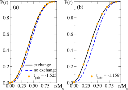
Figure 7: (color online) (a) GS cumulative probability $P(r)$ to find the two holes within a distance $r/M_{c}$ of each other, when magnon-exchange is allowed/forbidden (full/dashed lines). These are the same results as in Fig. 5. In addition, the symbols show $P(r)$ when the magnon-exchange is turned off but $H_{\rm eff}$ is added instead, with a $t_{\rm pair}=-1.525$. (b) Same as in (a) but for $U_{pp}=0$. In this case, $t_{\rm pair}=-1.156$.

We find that adding this $H_{\rm{eff}}$ to the calculation with magnon-exchange forbidden produces the same GS energy as the full calculation with the magnon-exchange allowed if we set $t_{\rm{pair}}=-1.525$. To validate it, in Fig. 7a we show that the GS cumulative probability in the enlarged space without magnon-exchange but with this $H_{\rm{eff}}$ included (symbols) matches perfectly that obtained when magnon-exchange is allowed (full line). This shows that this $H_{\rm{eff}}$ reproduces the GS wavefunction accurately. Furthermore, we find that it gives a faithful description of the effects of magnon-exchange in the entire Brillouin zone: Fig. 8 compares the differences $\Delta E_{\rm no-ex}=E_{\rm no-ex}-E_{\rm ex}$ and $\Delta E_{H_{\rm eff}}=E_{H_{\rm eff}}-E_{\rm ex}$ between the lowest eigenenergies without and with magnon-exchange (dashed line) versus the same difference but with $H_{\rm{eff}}$ included if magnon-exchange is forbidden (symbols). Note that $E_{ex}$ is shown in Fig. 2, as the lowest energy for each momentum in the Brillouin zone.

Clearly, $H_{\rm{eff}}$ reproduces very well the effect of the magnon-exchange in the full Brillouin zone, even though $t_{\rm pair}$ is fitted only for agreement at the $\Gamma$ point. Note that these energy variations are again due to the finite $M_{c}$ constraint. While the size of the energy differences depends on the value of $M_{c}$, we verified that adding this $H_{\rm{eff}}$ works well for any value of $M_{c}$.

We therefore conclude that this $H_{\rm{eff}}$ indeed reproduces very well the effect of the magnon-mediated attraction between the two holes. This is a non-trivial result, as there is no a priori reason to expect that $H_{\rm{eff}}$ contains a single class of processes. As mentioned, 2^nd order PT suggests three other possible candidates, involving $H_{J_{pd}}$ in the magnon emission and/or absorption. Although $H_{J_{pd}}$ and $T_{\rm{sw}}$ have comparable energy scales, these other processes turn out to have little effect, in other words higher order PT terms seem to renormalize them to become vanishingly small. We do not currently have a good understanding as to why this happens.

Of course, higher order PT terms also generate other possible exchange scenarios, involving more magnons. That these do not contribute much is less surprising because all their magnons have to be exchanged, i.e. created by a hole and absorbed by the other in a way that is not just a sequence of independent $H_{\rm{eff}}$ processes. This is rather difficult given the structure of the CuO₂ planes, which makes it easy for two holes to be neighbors of the same Cu spin, but impossible to be simulataneously neigbors of two or more different Cu spins.

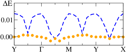
Figure 8: (color online) Differences between the lowest eigenenergies without and with magnon-exchange (dashed line) versus the same difference but with $H_{\rm{eff}}$ included when the magnon-exchange is turned-off (symbols).

The expression of this effective, magnon-mediated attraction $H_{\rm{eff}}$ is the central result of this work. It is very different from the more customary density-density or exchange type of effective interactions previously used in the literature. As such, it is likely to drive different behaviour at higher concentrations; investigation of these differences is left for future work.

Before concluding this section, we briefly address the dependence of $t_{\rm{pair}}$ on the various parameters. Most is as expected, eg. monotonic increase with both $t_{sw}$ and $J_{pd}$, shown in Figs. 9a,b respectively. The surprise is that $|t_{\rm{pair}}|$ increases with $U_{pp}$, see Fig. 9c. A larger $U_{pp}$ disfavors configurations with both holes on the same O, thus fewer pair-hopping+exchange processes are effectively allowed. Thus, it is not obvious whether the larger $|t_{\rm{pair}}|$ value really means stronger attraction because, at the same time, some terms in $H_{\rm eff}$ are effectively blocked. Indeed, the change in the cumulative probability with and without magnon-exchange is much more significant for $U_{pp}=0$ than that shown in Fig. 7b, suggesting that the magnon-mediated attraction is stronger for smaller $U_{pp}$. This serves to illustrate the fact that interactions like this $H_{\rm eff}$ have not been thoroughly studied and we lack intuition about their effects.

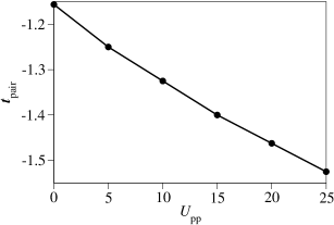
Figure 9: Dependence of $t_{\rm pair}$ on $t_{\rm sw}$ (top), on $J_{\rm pd}$ (middle) and $U_{pp}$ (bottom). In each case, all other parameters are held fixed at their stated values.

IV The role of background spin fluctuations

We have repeated the analysis described above in the case when spin-fluctuations (which allow any two adjacent, antiparallel Cu spins to simultaneouly flip their spins) are allowed within $m_{C}$ of the holes. This restriction is sensible because spin-fluctuations which occur far from the holes can be thought of as “vacuum fluctuations” with which the holes do not interact and which, therefore, will have no effect either on the holes’ dynamics or on the effective interaction between them.

In Ref. Ebrahimnejad et al., 2016 we proved that in the one-hole sector, this approach provides excellent agreement with Exact Diagonalization (which fully includes the effects of spin fluctuations) both for our three-band model, and for $t-t^{\prime}-t^{\prime\prime}-J$ one-band models. We also showed that spin fluctuations have no influence on the quasiparticle (spin-polaron) dynamics in the three-band model, even though they play an essential role in the one-band models. This is because as mentioned, in the three-band model $J_{dd}$ (which defines the characteristic timescale for spin-fluctuations) is significantly smaller than the other energy scales, whereas its counterpart $J$ in the one-band models is comparable to $t^{\prime},t^{\prime\prime}$ (for more analysis, see Ref. Ebrahimnejad et al., 2016).

Redoing the two-hole calculation in the presence of local spin-fluctuations reveals results very similar to those already discussed (not shown). In particular, the value of the best fit for $|t_{\rm pair}|$ varies by less that $5\%$. This clearly shows that the spin-fluctuations play little role in the effective attraction mediated by magnon-exchange, and validates our assertion that we can indeed ignore them.

This result is not surprising. As already mentioned several times, $J_{dd}$ is the smallest energy scale, meaning that spin-fluctuations happen on a very long (slow) time-scale. Roughly put, a magnon will be exchanged between holes much faster than the timescale over which spin fluctuations occur, which is why we can ignore them.

The same conclusion is reached if one tries to infer how spin-fluctuations might affect the magnon-exchange process. Suppose, for instance, that one of the holes flips its spin through either $H_{J_{pd}}$ or $T_{\rm sw}$ and creates a magnon at the Cu site denoted as ’1’. If this is the first magnon, then spin ’1’ is now parallel to its 4 Cu neighbors and spin-fluctuations cannot directly act on it. Spin fluctuations could flip another pair of neighboring spins (called ’2’ and ’3’) and then another spin fluctuation could flip two of them (eg, ’1’ and ’2’) back to their original orientations, leaving the magnon at site ’3’ (this sequence of events basically mimics magnon dispersion). The magnon can now be absorbed by the second hole. Clearly, this is a lot more complicated and less likely (for a small $J_{dd}$) than the simple process where one hole creates the magnon and the second absorbs it without further complications.

A simpler scenario is when there already exists a magnon on a Cu site neighbor to site ’1’, enabling a spin fluctuation involving spin ’1’ to occur without further complications. However, this will remove both magnons, so “magnon exchange” as normally envisioned would not occur. Nevertheless, if the other magnon was emitted by the other hole, then this process (and its counterpart, wherein a spin fluctuation creates two magnons, each of which is absorbed by a different hole) will contribute to the effective hole-hole interaction. Such processes are included in our calculation when local spin fluctuations are allowed and, as mentioned, were found to have only a tiny effect on the value of $t_{pair}$.

V On the existence of preformed pairs

So far, we found that for reasonable values of the parameters, the magnon-mediated interaction does not appear to be strong enough to bind the two holes into a preformed pair. To see how far away that regime is, we can increase $t_{\rm pair}$ by hand (thus mimicking a stronger magnon-mediated attraction) to find when binding occurs. An exact answer is difficult to obtain because of the finite maximum distance $M_{c}$ imposed between holes, which reduces the two-hole continuum to a fairly dense sequence of discrete levels. The value of $t_{\rm pair}$ where one state is pushed below this “continuum” changes somewhat with $M_{C}$, but we estimate that $|t_{\rm pair}|\sim 2.7$ is a safe upper limit – for this and larger values of $|t_{\rm pair}|$ the energy of the bound state is independent of $M_{c}$, and clearly well below the continuum.

Thus, the value $|t_{\rm pair}|=1.525$ we found is less than a factor of two from this critical value. This is very interesting because the rather small number of magnons kept in the variational space means that we overestimate the quasiparticle bandwidth by about the same factor, as shown in Figure 2 (the red lines are essentially converged, and show a significantly narrower bandwidth than the numerical results). Given that binding occurs when the lost kinetic energy is compensated by the increased attraction, this suggests that $t_{\rm pair}=-1.525$ may, in fact, be sufficient to weakly bind the two qps if their clouds are fully converged and they are somewhat slower/heavier. A definite answer will require significantly more work, as more magnons will need to be added in the variational space to fully converge the qps’ clouds when they are far from each other. We note that exact diagonalization of the same model on a 32Cu+64O cluster could not settle this issue either, because of considerable finite-size effects, Lau et al. (2011b) although those results also suggested that the system may be close to hosting pre-formed pairs.

This issue clearly deserves further, careful study, which we plan to attempt in the future. For now, we would like to speculate a bit more on this topic, because what we do know is already quite interesting.

First, the fact that our parameters seem so close to the critical region where pre-formed pairs may form suggests that on the BCS-BEC spectrum, superconductivity mediated by this $H_{\rm{eff}}$ would be more BEC than BCS-like, i.e. with pairs bound in real space, not in momentum space. Of course, the possibility of cuprate superconductivity emerging (at least on the underdoped side) when a liquid of preformed pairs becomes coherent has long been one of the leading scenarios.Corson et al. (2000a); Xu et al. (2000a); Tan and Levin (2008a); Yang et al. (2008a); Kanigel et al. (2008a); PF6 More recently, several groups have suggested that various unusual properties on the underdoped side can be explained as being due to the scattering of fermionic carriers on a bosonic liquid of preformed pairs.Jiang et al (2019a); Sacks et al (2017a, a) Our work seems to be consistent with these scenarios.

We leave it for future work to fully establish the symmetry of the preformed pairs (if they exist) and/or of our effective attraction. Note that the answer for the latter question is not trivial, because of the many-band structure and because of the form of the effective interaction. We can Fourier transform $H_{\rm eff}$, but (i) the potential will depend not just on the momentum ${\bf q}$ exchanged between the holes, but also on their total momentum ${\bf k+k^{\prime}}$. More importantly, (ii) because we have 4 different O sites in the magnetic unit cell, this potential is in fact a $4\times 4$ matrix, and its symmetry to rotations is more complicated to establish than for a scalar.

Even so, we can state that we expect this symmetry to be $d$-wave like. The reason is as follows. We know that for carriers moving on a square lattice like that made by the O ions, any amount of on-site ($s$-wave symmetry) attraction will lead to the appearance of a bound state. That we do not find this bound state when $U_{pp}>0$ may be explained by this being larger than the $s$-wave component of the effective attraction. However, we do not find a bound state even when $U_{pp}=0$. This can only mean that our effective interaction does not have a $s$-wave component, thus it is likely to be $d$-wave like.

VI Summary and conclusions

To conclude, we showed that magnon-exchange between holes doped in a cuprate layer leads to an effective attraction, and identified its expression $H_{\rm{eff}}$ and its energy scale $|t_{\rm pair}|\sim 1.5J_{dd}\sim 225$ meV.

The form of $H_{\rm{eff}}$ is unusual and requires further study. It is interesting that it has a “kinetic” nature, as the holes move while interacting. Evidence that pairing in cuprates comes through a “kinetic” mechanism was uncovered in optical experiments.O1-O5 As argued above, we also expect $H_{\rm{eff}}$ to favor pairs with $d$-wave symmetry, and to be strong enough so that the underdoped system either has pre-formed pairs, or is very close to it. If pre-formed pairs exist, they are very weakly bound, i.e. on a scale much smaller than $|t_{\rm pair}|$, consistent with the fact that both $T_{C}$ and the pseudogap temperature $T^{*}$ are well below $|t_{\rm pair}|$. Even if pre-formed pairs were unstable, the superconductivity promoted by $H_{\rm{eff}}$ is likely not BCS-like, but more towards BEC-like and unconventional.

As a final note, let us comment on why we expect this specific magnon-mediated effective attraction $H_{\rm{eff}}$, derived in the extremely underdoped limit and in the presence of LR AFM order, to be relevant at least in the whole underdoped regime. The answer is that this is interaction only involves the two holes and their common Cu spin through which they exchange the magnon. To first order it makes no difference whether this Cu spin is part of a magnetically ordered system or not, especially as all energy scales characterizing hole-spin interactions are much larger than $J_{dd}$. What may happen with increased hole concentration is that the magnitude $|t_{\rm pair}|$ of this effective interaction is renormalized, but we expect the functional form to remain the same.

Clearly, more work needs to be done to fully understand the consequences of this specific $H_{\rm{eff}}$ attraction, but we believe that the results reported here are interesting and intriguing, and warrant such further work.

Appendix A Hamiltonian details

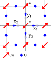
Figure 10: The CuO₂ lattice. The phase convention for the oxygen 2p orbitals is shown. Red arrows indicate the spin of the Cu-holes. The unit cell consists of the four oxygen sites marked with text and the two Cu-sites marked with an asterisk.

We study the model introduced by Lau et al. Lau et al. (2011a) in the two-hole sector, for a finite value of $U_{pp}$ (note that in Ref. Lau et al., 2011a, double occupancy is forbidden on the O sites). The holes propagate on the 2D CuO₂-layer depicted in Fig. 1a of the main article. In the $U_{dd}\rightarrow\infty$ limit at zero doping each Cu-ion is in a d⁹ configuration, i.e. hosts a single hole which is described by a spin-degree of freedom. Due to the superexchange interaction $H_{J_{dd}}$ (see below), these Cu-spins tend to align antiferromagnetically. As discussed in the main text, we first assume that this interaction is of Ising type and thus, in the absence of doped holes, the lattice of Cu-spins is in the Néel state. The role of the background spin-fluctuations enabled by the $x-y$ part of $H_{J_{dd}}$ is considered subsequently.

Starting from a Néel state, the magnetic unit cell comprises two Cu-sites and four oxygen sites. Our choice of unit cell is depicted in Fig. 10. For the $j^{\mathrm{th}}$ unit cell the lattice vector $\mathbf{R}_{j}$ points to the Cu_↓ site. The oxygen orbital $\alpha$ is located at $\mathbf{r}_{\alpha}=\mathbf{R}_{j}+\mathbf{u}_{\alpha}$ and the Cu_↑ site at $\mathbf{R}_{j}+a\hat{y}$, where $a$ is the lattice constant. It is convenient to measure distances in units of $a$/2, as we do from here on. Occasionally it will be convenient to sum over all the Cu_↑ sites. We will indicate this by $j\in\mathrm{Cu}_{\uparrow}$. In that case it is assumed that the vector $\mathbf{R}_{j}$ points to a Cu_↑ site. It then follows (see Fig. 10) that the neighboring oxygen orbital of type $\alpha$ is located at $\mathbf{R}_{j}-\mathbf{u}_{\alpha}$. If not otherwise stated, $\mathbf{R}_{j}$ is always assumed to point to a Cu_↓ site.

The two additional holes are hosted by the ligand oxygen $2p$-orbitals pointing towards the nearest Cu-ions. Their kinetic energy $T_{pp}$ is given by a tight binding Hamiltonian describing nearest neighbor (NN) and next nearest neighbor (NNN) hopping across Cu sites:

$$T_{pp}=t_{pp}\sum_{j,\sigma,\alpha,\mathbf{\delta}}\mathrm{s}(\mathbf{\delta})c_{j+\mathbf{u}_{\alpha}+\mathbf{\delta},\sigma}^{\dagger}c_{j+\mathbf{u}_{\alpha},\sigma}-t_{pp}^{\prime}\sum_{j,\sigma,\alpha}(c_{j+3\mathbf{u}_{\alpha},\sigma}^{\dagger}+c_{j-\mathbf{u}_{\alpha},\sigma}^{\dagger})c_{j+\mathbf{u}_{\alpha},\sigma}+\mathrm{H.c.}$$ (2)

Here $c_{j+\mathbf{u}_{\alpha},\sigma}^{\dagger}$ ($c_{j+\mathbf{u}_{\alpha},\sigma}$) creates (annihilates) a hole with spin $\sigma$ at site $\mathbf{R}_{j}+\mathbf{u}_{\alpha}$. The vectors $\mathbf{\delta}$ point to the four oxygen NN and $\mathrm{s}(\mathbf{\delta})$ is the sign of the corresponding hopping amplitude, listed in Tab. 1. These signs are for holes (not electrons) and can be inferred from the phases of the oxygen 2p orbitals depicted in Fig. 10. The positive constants $t_{pp}$ and $t_{pp}^{\prime}$ are the magnitudes of the NN and NNN hopping, respectively.

$\mathbf{\delta},\mathbf{\eta}$	$T_{pp}$	$T_{sw}$
(1,1)	+	-
(-1,1)	-	+
(-1,-1)	+	-
(1,-1)	-	+
(2,0)	-	-
(-2,0)	-	-
(0,2)	-	-
(0,-2)	-	-

Table 1: Hopping signs for $T_{pp}$ and $T_{sw}$. The vectors $\mathbf{\delta}$ and $\mathbf{\eta}$ are given in units of $a$/2. The first four rows are the NN hopping directions, while the NNN directions are listed in the rows below.

orbital $\alpha$	$\eta_{\alpha}$
x1	(-1,1) ; (-1,-1) ; (-2,0)
x2	(1,1) ; (1,-1) ; (2,0)
y1	(-1,-1) ; (1,-1) ; (0,-2)
y2	(-1,1) ; (1,1) ; (0,2)

Table 2: The vectors $\eta_{\alpha}$ pointing from orbital $\alpha$ to the oxygen orbitals which share a Cu_↓ neighbor (in units of $a$/2).

The interaction between holes and Cu-spins has two terms. The first is an exchange interaction:

$$H_{J_{pd}}=\sum_{\alpha}\left(\sum_{j\in\mathrm{Cu}_{\downarrow}}+\sum_{j\in\mathrm{Cu}_{\uparrow}}\right)\vec{s}_{j+\mathbf{u}_{\alpha}}\cdot\vec{S}_{j},$$ (3)

where $\vec{s}$ is the spin-operator for corresponding O holes and $\vec{S}$ is the spin-operator for the Cu-spins. The second term involves hopping of a hole while swapping its spin with the adjacent Cu:

$$T_{\rm sw} =t_{sw}\sum_{j\in\mathrm{Cu}-\downarrow}\sum_{\alpha,\sigma}\mathrm{s}(\eta_{\alpha})\left[c_{j+\mathbf{u}_{\alpha}+\eta_{\alpha},-\sigma}^{\dagger}S_{j}^{\sigma}(\frac{1}{2}-S_{j}^{z}\sigma)+c_{j+\mathbf{u}_{\alpha}+\eta_{\alpha},\sigma}^{\dagger}(\frac{1}{2}+S_{j}^{z}\sigma)\right]c_{j+\mathbf{u}_{\alpha},\sigma}$$

$$+t_{sw}\sum_{j\in\mathrm{Cu}-\uparrow}\sum_{\alpha,\sigma}\mathrm{s}(\eta_{\alpha})\left[c_{j-\mathbf{u}_{\alpha}-\eta_{\alpha},-\sigma}^{\dagger}S_{j}^{\sigma}(\frac{1}{2}-S_{j}^{z}\sigma)+c_{j-\mathbf{u}_{\alpha}-\eta_{\alpha},\sigma}^{\dagger}(\frac{1}{2}+S_{j}^{z}\sigma)\right]c_{j-\mathbf{u}_{\alpha},\sigma}$$ (4)

Here $S_{j}^{\pm}$ are the ladder operators for the Cu-spins. The vectors $\eta_{\alpha}$ point from orbital $\alpha$ to the other three oxygen orbitals adjacent to the same Cu_↓ site, see Tab. 2. The vectors $-\eta_{\alpha}$ point to the three O which share a Cu_↑ site with the orbital $\alpha$. Note, furthermore, that for $j\in\mathrm{Cu}_{\uparrow}$, the vector $-\mathbf{u}_{\alpha}$ points to orbital $\alpha$.

When on-site Coulomb interaction $U_{pp}$ between the holes is included, the magnitude of $t_{sw}$ for the terms which involve a doubly-occupied site as either the start or the final state, is renormalized by a factor $\frac{\Delta_{pd}+U_{pp}/2}{\Delta_{pd}+U_{pp}}$, where $\Delta_{pd}$ is the charge transfer gap. A derivation of this renormalization can be obtained using the perturbation theory as in Ref. Takahashi.

In the absence of holes, the Cu-Cu Ising interaction $\hat{H}_{J_{dd}}$ is given by

$$H_{J_{dd}}=J_{dd}\sum_{j}\sum_{\alpha}S_{j}^{z}S_{j+2\mathbf{u}_{\alpha}}^{z}$$ (5)

In the presence of doped holes it vanishes for those Cu-pairs which have one or more holes sitting on the O between them. In other words, the holes block the magnetic superexchange.

As mentioned, $H_{J_{dd}}$ is in fact of Heisenberg, not Ising type. The difference is that the former promotes an undoped ground-state which contains background spin-fluctuations, while the later has a Néel ground-state without any background spin-fluctuations. In a later section, we will show that these spin fluctuations have no effect on the magnon-mediated effective interaction between holes. This is achieved by allowing spin-fluctuations to occur in the vicinity of holes (effectively restoring $H_{J_{dd}}$ to its full Heisenberg form locally) and seeing if/how this affects the magnon-exchange. The first step, however, is to assume that there are no spin-fluctuations allowed, which we do from now on until specified otherwise.

Finally, including an on-site Hubbard interaction $U_{pp}$ between the holes, we arrive at the total Hamiltonian:

$$\mathcal{H}=T_{pp}+U_{pp}+T_{\rm sw}+H_{J_{pd}}+H_{J_{dd}}$$ (6)

We use the same parameters as in Ref. Lau et al., 2011a, which in units of $J_{dd}$ are $t_{pp}=4.13$, $t_{pp}^{\prime}=0.58t_{pp}$, $t_{sw}=2.98$ (2.20 for doubly occupied oxygen sites), $J_{pd}=2.83$, $U_{pp}=25.4$, $\Delta_{pd}=22.87$.

Appendix B Variational space details

To find the low-energy eigenstates we use a variational approach. This means that we restrict the Hilbert space to a physically meaningful subspace, termed the variational space (VS). In this variational space we can find the eigenstates, eigenenergies and Green’s functions using standard methods such as e.g. the Lanczos algorithm.

The first restriction imposed on the VS is the maximum number of magnons allowed, $n_{m}$. We are describing the Cu-spins as having an Ising exchange, so the magnons are dispersionless and correspond to Cu-spins which are flipped with respect to the Néel order (see main text discussion). For the single-hole case it was shown Ebrahimnejad et al. (2014, 2016) that reasonable convergence is already reached at $n_{m}=2$, because every magnon costs a finite energy of order $J_{dd}$, yet the magnons move very slowly compared to the holes, allowing us to neglect their dispersion.

Considering only states with up to two magnons we define the following translationally invariant basis states which span the VS:

$$|0,k,\mathbf{R},\mathbf{u}_{\alpha},\mathbf{u}_{\beta}\rangle=\sum_{j}\frac{\mathrm{e}^{i\mathbf{k}\mathbf{R}_{j}}}{\sqrt{N}}c_{j+\mathbf{u}_{\alpha},\uparrow}^{\dagger}c_{j+\mathbf{R}+\mathbf{u}_{\beta},\downarrow}^{\dagger}|0\rangle$$

$$|\sigma,k,\mathbf{r}_{\alpha},\mathbf{r}_{\beta}\rangle=\sum_{j}\frac{\mathrm{e}^{i\mathbf{k}\mathbf{R}_{j}}}{\sqrt{N}}c_{j+\mathbf{r}_{\alpha},-\sigma}^{\dagger}c_{j+\mathbf{r}_{\beta},-\sigma}^{\dagger}S_{j}^{\sigma}|0\rangle$$

$$|2,k,\mathbf{R},\mathbf{r}_{\alpha},\mathbf{r}_{\beta}\rangle=\sum_{j}\frac{\mathrm{e}^{i\mathbf{k}\mathbf{R}_{j}}}{\sqrt{N}}c_{j+\mathbf{r}_{\alpha},\uparrow}^{\dagger}c_{j+\mathbf{r}_{\beta},\downarrow}^{\dagger}S_{j}^{+}S_{j+\mathbf{R}+2\hat{y}}^{-}|0\rangle$$ (7)

Here $|0\rangle$ is the undoped Néel state and $N\rightarrow\infty$ denotes the number of lattice sites. All other quantities were defined in the preceding Section.

For all these states the distance between holes and/or magnons is well defined. For the zero-magnon and two-magnon states the holes have opposite spin and are therefore distinguishable. This is not true for the one-magnon states. In order to not double-count one-magnon states we require that $\mathbf{r}_{\alpha}$ is lexicographically smaller than $\mathbf{r}_{\beta}$.

For the zero-magnon states the reference unit cell is that of the $\uparrow$-hole, for the $\uparrow$-magnon and for the two-magnon states it is that of the $\uparrow$-magnon, and for the $\downarrow$-magnon states it is that of the $\downarrow$-magnon. These choices are convenient because the magnons do not move when we ignore the background spin-fluctuations.

To get a numerical solution, we need to further restrict the size of the VS. This is achieved by introducing two more cutoffs which are calculated using the L1 norm. The first is denoted by $M_{c}$ and restricts the distance between any two particles (particle refers to both holes and magnons). The second cutoff $m_{c}\leq M_{c}$ restricts the distance between a magnon and its closest hole. For example, for the zero-magnon states we require that $||\mathbf{R}+\mathbf{u}_{\beta}-\mathbf{u}_{\alpha}||_{1}\leq M_{c}$. Because no magnons are present, $m_{c}$ is irrelevant for the zero-magnon states.

A slightly more complicated example are the $\uparrow$-magnon states. The restriction $||\mathbf{R_{2}}+\mathbf{u}_{\beta}-\mathbf{R_{1}}-\mathbf{u}_{\alpha}||_{1}\leq M_{c}$ is always enforced. Furthermore one of the following sets of restrictions must also be enforced (i) $||\mathbf{R_{1}}+\mathbf{u}_{\alpha}||_{1}\leq m_{c}$ and $||\mathbf{R_{2}}+\mathbf{u}_{\beta}||_{1}\leq M_{c}$, or (ii) $||\mathbf{R_{2}}+\mathbf{u}_{\beta}||_{1}\leq m_{c}$ and $||\mathbf{R_{1}}+\mathbf{u}_{\alpha}||_{1}\leq M_{c}$. For the two-magnon states the restrictions are imposed in the same manner. Note that in this case it is possible that both magnons are within $m_{c}$ of the same hole.

As discussed in the main text, we turn off the magnon-mediated interactions by labelling the holes and magnons as being either flavor $a$ or $b$, and allowing each flavor of hole to interact only with its own flavor of magnon. Physical restrictions such as not allowing two magnons at the same Cu site are imposed, as further discussed below. The resulting states can easily be generalized from those in Eq. (7), as shown in Fig 1. (d) and (e).

For completeness, we now quickly review some aspects of the single-hole solution. The single-hole results shown here are identical to those from Refs Ebrahimnejad et al., 2014, 2016. The low-energy quasiparticle (QP) is a spin-polaron, i.e. a state in which the hole coherently emits and reabsorbs magnons. In Fig. 11 we show the qp dispersion, $\epsilon_{\mathrm{sp}}(\mathbf{k})$, along high symmetry lines of the BZ. Note that due to the AFM order of the Cu-spins, the BZ is reduced as shown in panel (b) of Fig. 11. As a result the $\Gamma$ and $M$ points are equivalent, as are X and Y.

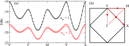
Figure 11: (a) The dispersion of the single hole along high symmetry lines of the BZ for a cutoff of $n_{m}=1$ and $n_{m}=2$. Lines are the fully converged solution ($m_{c}=20$) and circles are results for $m_{c}=3$. (b) A sketch of the cut in the BZ. The magnetic BZ is the small square.

For the single-hole solution we only need two cutoffs: $m_{c}$ (the hole-magnon distance) and $n_{m}$ (the maximum number of magnons). The solid lines in Fig. 11 are fully converged in $m_{c}$ while the open circles are for $m_{c}=3$. The effect of increasing $n_{m}$ from 1 to 2 is a constant energy shift and a decrease in bandwidth, while the shape of the dispersion remains similar. The single-hole calculation is essentially converged at $n_{m}=2$. Ebrahimnejad et al. (2014, 2016)

Appendix C Derivation of $H_{\mathrm{eff}}$

As described in the main text, we use second order perturbation theory (PT) to provide guidance for the possible types of terms that may arise when a magnon is exchanged between the two holes. To make sure that the magnon is truly exchanged, we have to work in the enlarged variational space where the holes and magnons have flavors so that we can distinguish direct processes (whereby the same hole creates and absorbs the magnon) from the exchange ones (where the magnon is created by one hole and absorbed by the other). We then project back to the physical space with $c,c^{\dagger}$ operators by using the physical antisymmetrical combinations that enforce Pauli’s principle. For example, the zero-magnon states are related by (also see Eq. 7):

$$|0,\mathbf{k},\mathbf{R},\mathbf{u}_{\alpha},\mathbf{u}_{\beta}\rangle \leftrightarrow\sum_{j}\frac{\mathrm{e}^{i\mathbf{k}\mathbf{R}_{j}}}{\sqrt{2N}}(a^{\dagger}_{j+\mathbf{u},_{\alpha}\uparrow}b^{\dagger}_{j+\mathbf{R}+\mathbf{u}_{\beta},\downarrow}-a^{\dagger}_{j+\mathbf{R}+\mathbf{u}_{\beta},\downarrow}b^{\dagger}_{j+\mathbf{u},_{\alpha}\uparrow})|0\rangle$$

$$\equiv\frac{1}{\sqrt{2}}[|0,\mathbf{k},\mathbf{R},\mathbf{u}_{\alpha}\uparrow,\mathbf{u}_{\beta}\downarrow\rangle_{E}-\mathrm{e}^{-i\mathbf{k}\mathbf{R}}|0,\mathbf{k},-\mathbf{R},\mathbf{u}_{\beta}\downarrow,\mathbf{u}_{\alpha}\uparrow\rangle_{E}]$$ (8)

where for convenience, we defined the zero-magnon states in the extended variational space:

$$|0,\mathbf{k},\mathbf{R},\mathbf{u}_{\alpha}\sigma,\mathbf{u}_{\beta}-\sigma\rangle_{E}=\sum_{j}\frac{\mathrm{e}^{i\mathbf{k}\mathbf{R}_{j}}}{\sqrt{N}}a^{\dagger}_{j+\mathbf{u}_{\alpha},\sigma}b^{\dagger}_{j+\mathbf{R}+\mathbf{u}_{\beta},-\sigma}|0\rangle$$ (9)

Next, we note that $H_{\mathrm{eff}}$ must be of the form $H_{\mathrm{eff}}=H_{\mathrm{eff}}^{\uparrow}+H_{\mathrm{eff}}^{\downarrow}$, where the superscript indicates whether an (originally) Cu_↑ or Cu_↓ is mediating the magnon exchange. These terms are schematically depicted in Fig. 12. Here we only show the terms which take a state from the $a_{\uparrow}b_{\downarrow}$-family to the $a_{\downarrow}b_{\uparrow}$-family. The other possible terms are just their Hermitian conjugates.

Finally, as mentioned in the main text, there are four possible kinds of terms in the full $H_{\mathrm{eff}}$, depending on whether the magnon is emitted and absorbed through $T_{\rm sw}$ and/or $J_{pd}$ processes (where one process is direct and the other is exchange). We have derived all these terms and analyzed each individually, as discussed in the main text. Because the term where both processes are of $T_{\rm sw}$ type turns out to dominate and to provide a faithful description of the magnon-exchange effects in the full Brillouin zone, in the following we focus on its derivation. All the other terms can be derived similarly.

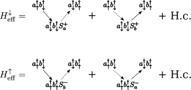
Figure 12: Sketch of the terms included in $H_{\mathrm{eff}}$. Solid (dashed) lines indicate normal (exchange) emission or absorption.

C.1 Derivation of $H_{\mathrm{eff}}^{\downarrow}$

Due to our choice of unit cell, it is easier to deal with $H_{\mathrm{eff}}^{\downarrow}$. The two terms depicted in Fig. 12 only differ by the magnon-label of the intermediate state. They therefore give the same result and we only need to consider the first term, which corresponds to first emitting with $T_{\mathrm{sw}}^{\mathrm{d}}$ and then reabsorbing with $T_{\mathrm{sw}}^{\mathrm{e}}$, where $d/e$ labels are for direct/exchange processes. Consequently, the effect of $H_{\mathrm{eff}}^{\downarrow}$ on the state $|0,\mathbf{k},\mathbf{R},\mathbf{u}_{\alpha}\uparrow,\mathbf{u}_{\beta}\downarrow\rangle_{E}$ is (see Eq. (A)):

$$H_{\mathrm{eff}}^{\downarrow}|0,\mathbf{k},\mathbf{R},\mathbf{u}_{\alpha}\uparrow,\mathbf{u}_{\beta}\downarrow\rangle_{E}=2t_{\mathrm{pair}}\delta_{\mathbf{R},0}\sum_{\begin{subarray}{c}\eta_{\alpha}\neq\\ \mathbf{u}_{\beta}-\mathbf{u}_{\alpha}\end{subarray}}\sum_{\eta_{\beta}}\mathrm{s}(\eta_{\alpha})\mathrm{s}(\eta_{\beta})|0,\mathbf{k},\mathbf{R},\mathbf{u}_{\alpha}+\eta_{\alpha}\downarrow,\mathbf{u}_{\beta}+\eta_{\beta}\uparrow\rangle_{E}$$ (10)

Here, as discussed in the main text, we leave $t_{\mathrm{pair}}$ as a parameter to be fitted, instead of using its PT expression. The restriction on $\eta_{\alpha}$ ensures that in the intermediate state where the holes have the same spin, they are not on the same site. Furthermore the holes need to sit on the “cage” surrounding a Cu-$\downarrow$ ion, which leads to the appearance of $\delta_{\mathbf{R},0}$. The result for the state $|0,\mathbf{k},-\mathbf{R},\mathbf{u}_{\beta}\downarrow,\mathbf{u}_{\alpha}\uparrow\rangle_{E}$ is derived similarly. Using the relationship of Eq. 8 between states in the extended variational space and those in the physical space, we then find:

$$H_{\mathrm{eff}}^{\downarrow}\sum_{j}\frac{\mathrm{e}^{i\mathbf{k}\mathbf{R}_{j}}}{\sqrt{N}}c_{j+\mathbf{u}_{\alpha},\uparrow}^{\dagger}c_{j+\mathbf{R}+\mathbf{u}_{\beta},\downarrow}^{\dagger}|0\rangle$$

$$=2t_{\mathrm{pair}}\delta_{\mathbf{R},0}\sum_{\begin{subarray}{c}\eta_{\alpha}\neq\\ \mathbf{u}_{\beta}-\mathbf{u}_{\alpha}\end{subarray}}\sum_{\eta_{\beta}}\mathrm{s}(\eta_{\alpha})\mathrm{s}(\eta_{\beta})\frac{1}{\sqrt{2}}[|0,\mathbf{k},\mathbf{R},\mathbf{u}_{\alpha}+\eta_{\alpha}\downarrow,\mathbf{u}_{\beta}+\eta_{\beta}\uparrow\rangle_{E}-\mathrm{e}^{-i\mathbf{k}\mathbf{R}}|0,\mathbf{k},\mathbf{-R},\mathbf{u}_{\beta}+\eta_{\beta}\uparrow,\mathbf{u}_{\alpha}+\eta_{\alpha}\downarrow\rangle_{E}]$$

$$=-2t_{\mathrm{pair}}\delta_{\mathbf{R},0}\sum_{\begin{subarray}{c}\eta_{\alpha}\neq\\ \mathbf{u}_{\beta}-\mathbf{u}_{\alpha}\end{subarray}}\sum_{\eta_{\beta}}\mathrm{s}(\eta_{\alpha})\mathrm{s}(\eta_{\beta})\frac{\mathrm{e}^{-i\mathbf{k}\mathbf{R}}}{\sqrt{2}}[|0,\mathbf{k},\mathbf{-R},\mathbf{u}_{\beta}+\eta_{\beta}\uparrow,\mathbf{u}_{\alpha}+\eta_{\alpha}\downarrow\rangle_{E}-\mathrm{e}^{i\mathbf{k}\mathbf{R}}|0,\mathbf{k},\mathbf{R},\mathbf{u}_{\alpha}+\eta_{\alpha}\downarrow,\mathbf{u}_{\beta}+\eta_{\beta}\uparrow\rangle_{E}]$$

$$=-2t_{\mathrm{pair}}\delta_{\mathbf{R},0}\sum_{\begin{subarray}{c}\eta_{\alpha}\neq\\ \mathbf{u}_{\beta}-\mathbf{u}_{\alpha}\end{subarray}}\sum_{\eta_{\beta}}\mathrm{s}(\eta_{\alpha})\mathrm{s}(\eta_{\beta})\mathrm{e}^{-i\mathbf{k}\mathbf{R}}\sum_{j}\frac{\mathrm{e}^{i\mathbf{k}\mathbf{R}_{j}}}{\sqrt{N}}c_{j+\mathbf{u}_{\beta}+\eta_{\beta},\uparrow}^{\dagger}c_{j-\mathbf{R}+\mathbf{u}_{\alpha}+\eta_{\alpha},\downarrow}^{\dagger}|0\rangle$$ (11)

This holds for any choice of $\alpha$ and $\beta$, therefore we can immediately read off that $H_{\mathrm{eff}}^{\downarrow}$ must have the form listed in the main text:

$$H_{\mathrm{eff}}^{\downarrow}=-2t_{\mathrm{pair}}\delta_{\mathbf{R},0}\sum_{j}\sum_{\alpha,\beta}\sum_{\begin{subarray}{c}\eta_{\alpha}\neq\\ \mathbf{u}_{\beta}-\mathbf{u}_{\alpha}\end{subarray}}\sum_{\eta_{\beta}}\mathrm{s}(\eta_{\alpha})\mathrm{s}(\eta_{\beta})c_{j+\mathbf{u}_{\beta}+\eta_{\beta},\uparrow}^{\dagger}c_{j+\mathbf{u}_{\alpha}+\eta_{\alpha},\downarrow}^{\dagger}c_{j+\mathbf{u}_{\beta},\downarrow}c_{j+\mathbf{u}_{\alpha},\uparrow}$$ (12)

C.2 Derivation of $H_{\mathrm{eff}}^{\uparrow}$

To obtain an expression for $H_{\mathrm{eff}}^{\uparrow}$ we first rewrite $|0,\mathbf{k},\mathbf{R},\mathbf{u}_{\alpha}\uparrow,\mathbf{u}_{\beta}\downarrow\rangle_{E}\rangle$ (where the sum is over Cu_↓ sites by definition) so that the sum is over Cu_↑ sites instead. The Cu_↑ site at $\mathbf{R}_{j}+2\mathbf{u}_{\alpha}$ is closest to the ’a’ hole at $\mathbf{R}_{j}+\mathbf{u}_{\alpha}$. Consequently we make the substitution $R_{j^{\prime}}=\mathbf{R}_{j}+2\mathbf{u}_{\alpha}$ which yields

$$|0,\mathbf{k},\mathbf{R},\mathbf{u}_{\alpha}\uparrow,\mathbf{u}_{\beta}\downarrow\rangle_{E}=\sum_{j^{\prime}\in\mathrm{Cu}_{\uparrow}}\frac{\mathrm{e}^{i\mathbf{k}(\mathbf{R}_{j^{\prime}}-2\mathbf{u}_{\alpha})}}{\sqrt{N}}\phi_{a,\uparrow}(\mathbf{R}_{j^{\prime}}-\mathbf{u}_{\alpha})\phi_{b,\downarrow}(\mathbf{R}_{j^{\prime}}+\mathbf{R}-2\mathbf{u}_{\alpha}+2\mathbf{u}_{\beta}-\mathbf{u}_{\beta})|0\rangle.$$ (13)

Before we continue the following observations are helpful. The site $\mathbf{R}_{j^{\prime}}-\mathbf{u}_{\alpha}$ is still the site of an $\alpha$ orbital. Furthermore the vector $2\mathbf{u}_{\alpha}-2\mathbf{u}_{\beta}$ is a lattice vector so that we must have $\mathbf{R}=2\mathbf{u}_{\alpha}-2\mathbf{u}_{\beta}$ in order for the two holes to share the same Cu_↑ neighbor.

To calculate the effect of $H_{\mathrm{eff}}^{\uparrow}$ we make use of the fact that from an orbital of type $\alpha$, the vectors $-\eta_{\alpha}$ point to the sites which can be reached by “hopping over” the NN Cu_↑ site. We then obtain:

$$H_{\mathrm{eff}}^{\uparrow}|0,\mathbf{k},\mathbf{R},\mathbf{u}_{\alpha}\uparrow,\mathbf{u}_{\beta}\downarrow\rangle_{E}$$

$$=2t_{\mathrm{pair}}\delta_{\mathbf{R},2\mathbf{u}_{\alpha}-2\mathbf{u}_{\beta}}\sum_{\begin{subarray}{c}\eta_{\beta}\neq\\ \mathbf{u}_{\alpha}-\mathbf{u}_{\beta}\end{subarray}}\sum_{\eta_{\alpha}}\mathrm{s}(-\eta_{\beta})\mathrm{s}(-\eta_{\alpha})\sum_{j^{\prime}\in\mathrm{Cu}_{\uparrow}}\frac{\mathrm{e}^{i\mathbf{k}(\mathbf{R}_{j^{\prime}}-2\mathbf{u}_{\alpha})}}{\sqrt{N}}\phi_{a,\downarrow}(\mathbf{R}_{j^{\prime}}-\mathbf{u}_{\alpha}-\eta_{\alpha})\phi_{b,\uparrow}(\mathbf{R}_{j^{\prime}}-\mathbf{u}_{\beta}-\eta_{\beta})|0\rangle.$$ (14)

We now have to rewrite this back as a sum over Cu_↓ sites. To do this we make the substitution $\mathbf{R}_{j}=\mathbf{R}_{j^{\prime}}-2\mathbf{u}_{\alpha}-2\eta_{\alpha}$. This gives:

$$H_{\mathrm{eff}}^{\uparrow}|0,\mathbf{k},\mathbf{R},\mathbf{u}_{\alpha}\uparrow,\mathbf{u}_{\beta}\downarrow\rangle_{E}$$

$$=2t_{\mathrm{pair}}\delta_{\mathbf{R},2\mathbf{u}_{\alpha}-2\mathbf{u}_{\beta}}\sum_{\begin{subarray}{c}\eta_{\beta}\neq\\ \mathbf{u}_{\alpha}-\mathbf{u}_{\beta}\end{subarray}}\sum_{\eta_{\alpha}}e^{2i\mathbf{k}\eta_{\alpha}}\mathrm{s}(-\eta_{\beta})\mathrm{s}(-\eta_{\alpha})|0,\mathbf{k},\mathbf{R}+2\eta_{\alpha}-2\eta_{\beta},\mathbf{u}_{\alpha}+\eta_{\alpha}\downarrow,\mathbf{u}_{\beta}+\eta_{\beta},\uparrow\rangle_{E}$$ (15)

A similar calculation yields

$$H_{\mathrm{eff}}^{\uparrow}|0,\mathbf{k},-\mathbf{R},\mathbf{u}_{\beta}\downarrow,\mathbf{u}_{\alpha}\uparrow\rangle_{E}$$

$$=2t_{\mathrm{pair}}\delta_{\mathbf{R},2\mathbf{u}_{\alpha}-2\mathbf{u}_{\beta}}\sum_{\begin{subarray}{c}\eta_{\beta}\neq\\ \mathbf{u}_{\alpha}-\mathbf{u}_{\beta}\end{subarray}}\sum_{\eta_{\alpha}}\mathrm{s}(-\eta_{\beta})\mathrm{s}(-\eta_{\alpha})\mathrm{e}^{2i\mathbf{k}\eta_{\beta}}|0,\mathbf{k},-\mathbf{R}+2\eta_{\beta}-2\eta_{\alpha},\mathbf{u}_{\beta}+\eta_{\beta}\uparrow,\mathbf{u}_{\alpha}+\eta_{\alpha}\downarrow\rangle_{E}$$ (16)

Making use of Eq. (8), the effect of $H_{\mathrm{eff}}^{\uparrow}$ in the language of the $c$-operators is:

$$H_{\mathrm{eff}}^{\uparrow} \sum_{j}\mathrm{e}^{i\mathbf{k}\mathbf{R}_{j}}c_{j+\mathbf{u}_{\alpha},\uparrow}^{\dagger}c_{j+\mathbf{R}+\mathbf{u}_{\beta},\downarrow}^{\dagger}|0\rangle$$

$$= 2t_{\mathrm{pair}}\delta_{\mathbf{R},2\mathbf{u}_{\alpha}-2\mathbf{u}_{\beta}}\sum_{\begin{subarray}{c}\eta_{\beta}\neq\\ \mathbf{u}_{\alpha}-\mathbf{u}_{\beta}\end{subarray}}\sum_{\eta_{\alpha}}\mathrm{s}(-\eta_{\beta})\mathrm{s}(-\eta_{\alpha})\frac{1}{\sqrt{2}}[\mathrm{e}^{2i\mathbf{k}\eta_{\alpha}}|0,\mathbf{k},\mathbf{R}+2\eta_{\alpha}-2\eta_{\beta},\mathbf{u}_{\alpha}+\eta_{\alpha}\downarrow,\mathbf{u}_{\beta}+\eta_{\beta}\uparrow\rangle_{E}$$

$$-\mathrm{e}^{2i\mathbf{k}\eta_{\beta}-i\mathbf{k}\mathbf{R}}|0,\mathbf{k},-\mathbf{R}+2\eta_{\beta}-2\eta_{\alpha},\mathbf{u}_{\beta}+\eta_{\beta}\uparrow,\mathbf{u}_{\alpha}+\eta_{\alpha}\downarrow\rangle_{E}]$$

$$= -2t_{\mathrm{pair}}\delta_{\mathbf{R},2\mathbf{u}_{\alpha}-2\mathbf{u}_{\beta}}\sum_{\begin{subarray}{c}\eta_{\beta}\neq\\ \mathbf{u}_{\alpha}-\mathbf{u}_{\beta}\end{subarray}}\sum_{\eta_{\alpha}}\mathrm{s}(-\eta_{\beta})\mathrm{s}(-\eta_{\alpha})\frac{\mathrm{e}^{2i\mathbf{k}\eta_{\beta}-i\mathbf{k}\mathbf{R}}}{\sqrt{2}}[|0,\mathbf{k},-\mathbf{R}+2\eta_{\beta}-2\eta_{\alpha},\mathbf{u}_{\beta}+\eta_{\beta}\uparrow,\mathbf{u}_{\alpha}+\eta_{\alpha}\downarrow\rangle_{E}$$

$$-\mathrm{e}^{i\mathbf{k}(\mathbf{R}+2\eta_{\alpha}-2\eta_{\beta})}|0,\mathbf{k},\mathbf{R}+2\eta_{\alpha}-2\eta_{\beta},\mathbf{u}_{\alpha}+\eta_{\alpha}\downarrow,\mathbf{u}_{\beta}+\eta_{\beta}\uparrow\rangle_{E}]$$

$$= -2t_{\mathrm{pair}}\delta_{\mathbf{R},2\mathbf{u}_{\alpha}-2\mathbf{u}_{\beta}}\sum_{\begin{subarray}{c}\eta_{\beta}\neq\\ \mathbf{u}_{\alpha}-\mathbf{u}_{\beta}\end{subarray}}\sum_{\eta_{\alpha}}\mathrm{s}(-\eta_{\beta})\mathrm{s}(-\eta_{\alpha})\mathrm{e}^{2i\mathbf{k}\eta_{\beta}-i\mathbf{k}\mathbf{R}}\sum_{j}\mathrm{e}^{i\mathbf{k}\mathbf{R}_{j}}c_{j+\mathbf{u}_{\beta}+\eta_{\beta},\uparrow}^{\dagger}c_{j-\mathbf{R}+2\eta_{\beta}-2\eta_{\alpha}+\mathbf{u}_{\alpha}+\eta_{\alpha},\downarrow}^{\dagger}|0\rangle$$ (17)

To read off an expression for $H_{\mathrm{eff}}^{\uparrow}$ we transform the sums over $j$ on both sides of the equation so that $\mathbf{R}_{j}\in$ Cu_↑. For the sum on the left hand side this is achieved with the substitution $\mathbf{R}_{j^{\prime}}=\mathbf{R}_{j}+2\mathbf{u}_{\alpha}$. For the sum on the right hand side we substitute $\mathbf{R}_{j^{\prime}}=\mathbf{R}_{j}+2\mathbf{u}_{\beta}+2\eta_{\beta}$.

$$\sum_{j^{\prime}\in\mathrm{Cu}_{\uparrow}}H_{\mathrm{eff}}^{\uparrow}\mathrm{e}^{i\mathbf{k}(\mathbf{R}_{j^{\prime}}-2\mathbf{u}_{\alpha})}c_{j^{\prime}-\mathbf{u}_{\alpha},\uparrow}^{\dagger}c_{j^{\prime}+\mathbf{R}-2\mathbf{u}_{\alpha}+2\mathbf{u}_{\beta}-\mathbf{u}_{\beta},\downarrow}^{\dagger}|0\rangle$$

$$= -2t_{\mathrm{pair}}\delta_{\mathbf{R},2\mathbf{u}_{\alpha}-2\mathbf{u}_{\beta}}\sum_{\begin{subarray}{c}\eta_{\beta}\neq\\ \mathbf{u}_{\alpha}-\mathbf{u}_{\beta}\end{subarray}}\sum_{\eta_{\alpha}}\mathrm{s}(-\eta_{\beta})\mathrm{s}(-\eta_{\alpha})\mathrm{e}^{2i\mathbf{k}\eta_{\beta}-i\mathbf{k}\mathbf{R}}\sum_{j^{\prime}\in\mathrm{Cu}_{\uparrow}}\mathrm{e}^{i\mathbf{k}(\mathbf{R}_{j^{\prime}}-2\mathbf{u}_{\beta}-2\eta_{\beta})}c_{j^{\prime}-\mathbf{u}_{\beta}-\eta_{\beta},\uparrow}^{\dagger}c_{j^{\prime}-\mathbf{R}+2\mathbf{u}_{\alpha}-2\mathbf{u}_{\beta}-\mathbf{u}_{\alpha}-\eta_{\alpha},\downarrow}^{\dagger}|0\rangle$$ (18)

Note that when we make use of the $\delta$-function, $\mathbf{R}$ cancels out and the terms in the exponential cancel as well, so that we obtain:

$$\sum_{j^{\prime}\in\mathrm{Cu}_{\uparrow}}\mathrm{e}^{i\mathbf{k}\mathbf{R}_{j^{\prime}}}[H_{\mathrm{eff}}^{\uparrow}c_{j^{\prime}-\mathbf{u}_{\alpha},\uparrow}^{\dagger}c_{j^{\prime}-\mathbf{u}_{\beta},\downarrow}^{\dagger}|0\rangle+2t_{\mathrm{pair}}\sum_{\begin{subarray}{c}\eta_{\beta}\neq\\ \mathbf{u}_{\alpha}-\mathbf{u}_{\beta}\end{subarray}}\sum_{\eta_{\alpha}}\mathrm{s}(-\eta_{\beta})\mathrm{s}(-\eta_{\alpha})c_{j^{\prime}-\mathbf{u}_{\beta}-\eta_{\beta},\uparrow}^{\dagger}c_{j^{\prime}-\mathbf{u}_{\alpha}-\eta_{\alpha},\downarrow}^{\dagger}|0\rangle]=0$$ (19)

Consequently we must have

$$H_{\mathrm{eff}}^{\uparrow}=2t_{\mathrm{pair}}\sum_{j\in\mathrm{Cu}_{\uparrow}}\sum_{\alpha,\beta}\sum_{\begin{subarray}{c}\eta_{\beta}\neq\\ \mathbf{u}_{\alpha}-\mathbf{u}_{\beta}\end{subarray}}\sum_{\eta_{\alpha}}\mathrm{s}(-\eta_{\beta})\mathrm{s}(-\eta_{\alpha})c_{j-\mathbf{u}_{\beta}-\eta_{\beta},\uparrow}^{\dagger}c_{j-\mathbf{u}_{\alpha}-\eta_{\alpha},\downarrow}^{\dagger}c_{j-\mathbf{u}_{\beta},\downarrow}c_{j-\mathbf{u}_{\alpha},\uparrow}$$ (20)

Note that this expression is essentially the same as for $H_{\mathrm{eff}}^{\downarrow}$, but with the first sum running over all the Cu_↑ sites instead of the Cu_↓ sites. That is in agreement with what is expected by symmetry, validating these derivations.

References

- Bednorz and Müller (1986) J. G. Bednorz and K. A. Müller, Zeitschrift für Physik B Condensed Matter 64, 189 (1986), URL https://doi.org/10.1007/BF01303701.
- Anderson (2007) P. W. Anderson, Science 316, 1705 (2007), ISSN 0036-8075, URL http://science.sciencemag.org/content/316/5832/1705.
- Bardeen, Cooper and Schrieffer (1957) J. Bardeen, L. N. Cooper and J. R. Schrieffer, Physical Review 106, 162-164 (1957), URL https://journals.aps.org/pr/abstract/10.1103/PhysRev.106.162.
- Alexandrov and Mott (1994) A. S. Alexandrov and N. F. Mott, Reports on Progress in Physics 57, 1197 (1994), URL http://stacks.iop.org/0034-4885/57/i=12/a=001.
- Alexandrov (2009) A. S. Alexandrov, Journal of Superconductivity and Novel Magnetism 22, 103 (2009), ISSN 1557-1947, URL https://doi.org/10.1007/s10948-008-0393-1.
- Kresin and Wolf (2009) V. Kresin and S. Wolf, Rev. Mod. Phys. 81, 481 (2009), URL https://journals.aps.org/rmp/pdf/10.1103/RevModPhys.81.481.
- Moriya and Ueda (2000) T. Moriya and K. Ueda, Advances in Physics 49, 555 (2000), URL https://doi.org/10.1080/000187300412248.
- Lee et al. (2006) P. A. Lee, N. Nagaosa, and X.-G. Wen, Rev. Mod. Phys. 78, 17 (2006), URL https://link.aps.org/doi/10.1103/RevModPhys.78.17.
- Ogata and Fukuyama (2008) M. Ogata and H. Fukuyama, Reports on Progress in Physics 71, 036501 (2008), URL http://stacks.iop.org/0034-4885/71/i=3/a=036501.
- Monthoux et al. (2007) P. Monthoux, D. Pines, and G. Lonzarich, Nature 450, 1177 (2007), URL https://www.nature.com/articles/nature06480.
- Val’kov and Barabanov (2016) D. Val’kov, V.V. abd Dzebisashvili and A. Barabanov, JETP Lett. 104, 730 (2016), URL https://link.aps.org/doi/10.1103/PhysRevB.90.184515.
- Dai (2015) P. Dai, Rev. Mod. Phys. 87, 855 (2015), URL https://link.aps.org/doi/10.1103/RevModPhys.87.855.
- Stewart (1984) G. R. Stewart, Rev. Mod. Phys. 56, 755 (1984), URL https://link.aps.org/doi/10.1103/RevModPhys.56.755.
- Varma (2006) C. M. Varma, Phys. Rev. B 73, 155113 (2006), URL https://doi.org/10.1134/S002136401622015X.
- Hirsch (2014) J. E. Hirsch, Phys. Rev. B 90, 184515 (2014), URL https://link.aps.org/doi/10.1103/PhysRevB.90.184515.
- Sakai et al. (2016) S. Sakai, M. Civelli, and M. Imada, Phys. Rev. Lett. 116, 057003 (2016), URL https://link.aps.org/doi/10.1103/PhysRevLett.116.057003.
- Cataudella et al. (2007) V. Cataudella, G. De Filippis, A. S. Mishchenko, and N. Nagaosa, Phys. Rev. Lett. 99, 226402 (2007), URL https://link.aps.org/doi/10.1103/PhysRevLett.99.226402.
- Dal Conte et al. (2012) S. Dal Conte, C. Giannetti, G. Coslovitch, F. Cilento, D. Bossini, T. Abebaw, F. Banfi, G. Ferrini, H. Eisaki, M. Greven, et al., Science 335, 1600 (2012), URL http://science.sciencemag.org/content/335/6076/1600.full.
- Emery (1987) V. J. Emery, Phys. Rev. Lett. 58, 2794 (1987), URL https://link.aps.org/doi/10.1103/PhysRevLett.58.2794.
- (20) Models similar to ours are used in both Zaanen, J. and Oles, A.M. Canonical perturbation theory and the two-band model for high-Tc superconductors Phys. Rev. B 37, 9423 – 9438 (1988); and in Ding, H.-Q., Lang, G.H. and Goddard, III, W.A. Band structure, magnetic fluctuations, and quasiparticle nature of the two-dimensional three-band Hubbard model Phys. Rev. B 46, 14317 – 14320 (1992), however in one-dimension (former) or for a cluster (latter).
- Zhang and Rice (1988) F. C. Zhang and T. M. Rice, Phys. Rev. B 37, 3759 (1988), URL https://link.aps.org/doi/10.1103/PhysRevB.37.3759.
- Eskes and Sawatzky (1988) H. Eskes and G. A. Sawatzky, Phys. Rev. Lett. 61, 1415 (1988), URL https://link.aps.org/doi/10.1103/PhysRevLett.61.1415.
- Moeller et al. (2012a) M. M. Möller, G. A. Sawatzky, and M. Berciu, Phys. Rev. Lett. 108, 216403 (2012a), URL https://link.aps.org/doi/10.1103/PhysRevLett.108.216403.
- Ebrahimnejad et al. (2014) H. Ebrahimnejad, G. A. Sawatzky, and M. Berciu, Nature Physics 10, 951 (2014), URL http://dx.doi.org/10.1038/nphys3130.
- Ebrahimnejad et al. (2016) H. Ebrahimnejad, G. A. Sawatzky, and M. Berciu, Journal of Physics: Condensed Matter 28, 105603 (2016), URL http://stacks.iop.org/0953-8984/28/i=10/a=105603.
- Lau et al. (2011a) B. Lau, M. Berciu, and G. A. Sawatzky, Phys. Rev. Lett. 106, 036401 (2011a), URL https://link.aps.org/doi/10.1103/PhysRevLett.106.036401.
- (27) M. M. Möller and M. Berciu, unpublished.
- Lau et al. (2011b) B. Lau, M. Berciu, and G. A. Sawatzky, Phys. Rev. B 84, 165102 (2011b), URL https://link.aps.org/doi/10.1103/PhysRevB.84.165102.
- Corson et al. (2000a) J. Corson, R. Mallozzi, J. Orenstein, J. N. Eckstein, and I. Bozovic, Nature 398, 221-223 (1999a), URL https://www.nature.com/articles/18402.
- Xu et al. (2000a) Z. A.. Xu, N. P. Ong, Y Wang, T. Kakeshita, and S. Uchida, Nature 406, 486-488 (2000a), URL https://www.nature.com/articles/35020016.
- Tan and Levin (2008a) S. Tan, and K. Levin, Phys. Rev. B 69, 064510 (2004a), URL https://journals.aps.org/prb/abstract/10.1103/PhysRevB.69.064510.
- Yang et al. (2008a) H.-B. Yang, J.D. Rameau, P.F. Johnson, T. Valla, A. Tsvelik, and G. D. Gu, Nature 456, 77-80 (2008a), URL https://www.nature.com/articles/nature07400.
- Kanigel et al. (2008a) A. Kanigel, U. Chatterjee, M. Randeria, M. R. Norman, G. Koren, K. Kadowaki, and J. C. Campuzano, Phys. Rev. Lett. 101, 137002 (2008a), URL https://journals.aps.org/prl/abstract/10.1103/PhysRevLett.101.137002.
- (34) M. Shi et al., EuroPhys. Lett. 88, 27008 (2009a), URL https://iopscience.iop.org/article/10.1209/0295-5075/88/27008.
- Jiang et al (2019a) S. Jiang, L. Zou, and W. Ku, Phys. Rev. B 99, 104507 (2019a), URL https://journals.aps.org/prb/abstract/10.1103/PhysRevB.99.104507.
- Sacks et al (2017a) W. Sacks, A. Mauger, and Y. N. Noat, EuroPhys. Lett. 119, 17001 (2017a), URL https://iopscience.iop.org/article/10.1209/0295-5075/119/17001.
- Sacks et al (2017a) W. Sacks, A. Mauger, and Y. N. Noat, Sol. State Comm. 257, 1-5 (2017a), URL https://doi.org/10.1016/j.ssc.2017.03.009.
- (38) J. E. Hirsch, Physica C 199, 305-310 (1992), URL https://www.sciencedirect.com/science/article/abs/pii/0921453492904159.
- (39) S. Chakravarty, A. Sudbo, P. A. Anderson, and S. Strong, Science 261, 337-340 (1993), URL https://science.sciencemag.org/content/261/5119/337.
- (40) V. J. Emery, S. A. Kiverlson, and O. Zachar, Phys. Rev. B 56, 6120 (1997), URL https://journals.aps.org/prb/abstract/10.1103/PhysRevB.56.6120.
- (41) D. van der Marel, A. J. Leggett, J. W. Loram, and J. R. Kirtley, Phys. Rev. B 66, 140501(R) (2002), URL https://journals.aps.org/prb/abstract/10.1103/PhysRevB.66.140501.