Spectral properties of kernel matrices
in the flat limit

Abstract

Kernel matrices are of central importance to many applied fields. In this manuscript, we focus on spectral properties of kernel matrices in the so-called “flat limit”, which occurs when points are close together relative to the scale of the kernel. We establish asymptotic expressions for the determinants of the kernel matrices, which we then leverage to obtain asymptotic expressions for the main terms of the eigenvalues. Analyticity of the eigenprojectors yields expressions for limiting eigenvectors, which are strongly tied to discrete orthogonal polynomials. Both smooth and finitely smooth kernels are covered, with stronger results available in the finite smoothness case.

15A18, 47A55, 47A75, 47B34, 60G15, 65D05

1 Introduction

For an ordered set of points $\mathcal{X}=(\bm{x}_{1},\ldots,\bm{x}_{n})$, $\bm{x}_{k}\in\Omega\subset\mathbb{R}^{d}$, not lying in general on a regular grid, and a kernel $K:\Omega\times\Omega\to\mathbb{R}$, the kernel matrix $\bm{K}$ is defined as

$$\bm{K}=\bm{K}(\mathcal{X})=\left[K(\bm{x}_{i},\bm{x}_{j})\right]_{i,j=1}^{n,n}.$$

These matrices occur in approximation theory (kernel-based approximation and interpolation, [33, 43]), statistics and machine learning (Gaussian process models [44], Support Vector Machines and kernel PCA [34]).

Often, a positive scaling parameter is introduced, and the scaled kernel matrix becomes

(1) $$\bm{K}_{\varepsilon}=\bm{K}_{\varepsilon}(\mathcal{X})=\left[\color[rgb]{0,0,0}K_{\varepsilon}(\bm{x}_{i},\bm{x}_{j})\color[rgb]{0,0,0}\right]_{i,j=1}^{n,n},\color[rgb]{0,0,0}$$

where typically $K_{\varepsilon}(\bm{x},\bm{y})=K(\varepsilon\bm{x},\varepsilon\bm{y})$. If the kernel is radial (the most common case), then its value depends only on the Euclidean distance between $\bm{x}$ and $\bm{y}$, and $\varepsilon$ determines how quickly the kernel decays with distance.

Understanding spectral properties of kernel matrices is essential in statistical applications (e.g., for selecting hyperparameters), as well as in scientific computing (e.g., for preconditioning [13, 41]). Because the spectral properties of kernel matrices are not directly tractable in the general case, one usually needs to resort to asymptotic results. The most common form of asymptotic analysis takes $n\rightarrow\infty$. Three cases are typically considered: (a) when the distribution of points in $\mathcal{X}$ converges to some continuous measure on $\Omega$, the kernel matrix tends in some sense to a linear operator in a Hilbert space, whose spectrum is then studied [39]; (b) recently, some authors have obtained asymptotic results in a regime where both $n$ and the dimension $d$ tend to infinity [11, 7, 40], using the tools of random matrix theory; (c) in a special case of $\mathcal{X}$ lying on a regular grid, stationary kernel matrices become Toeplitz or more generally multilevel Toeplitz, whose asymptotic spectral distribution are determined by their symbol (or the Fourier transform of the sequence) [18, 2, 38, 29, 3].

Driscoll & Fornberg [10] pioneered a new form of asymptotic analysis for kernel methods, in the context of Radial Basis Function (RBF) interpolation. The point set $\mathcal{X}$ is considered fixed, with arbitrary geometry (i.e., not lying in general on a regular grid), and the scaling parameter $\varepsilon$ approaches $0$. Driscoll & Fornberg called this the “flat limit”, as kernel functions become flat over the range of $\mathcal{X}$ as $\varepsilon\rightarrow 0$. Very surprisingly, they showed that for certain kernels the RBF interpolant stays well-defined in the flat limit, and tends to the Lagrange polynomial interpolant. Later, a series of papers extended their results to the multivariate case [31, 24, 32] and established similar convergence results for various types of radial functions (see [35, 27] and references therein). In particular, [35] showed that for kernels of finite smoothness the limiting interpolant is a spline rather than a polynomial.

The flat limit is interesting for several reasons. In contrast to other asymptotic analyses, it is deterministic ($\mathcal{X}$ is fixed), and makes very few assumptions on the geometry of the point set. In addition, kernel methods are plagued by the problem of picking a scale parameter [34]. One either uses burdensome procedures like cross-validation or maximum likelihood [44] or sub-optimal but cheap heuristics like the median distance heuristic [16]. The flat limit analysis may shed some light on the problem. Finally, the results derived here can be thought of as perturbation results, in the sense that they are formally exact in the limit, but useful approximations when the scale is not too small.

Despite its importance, little was known until recently about the eigenstructure of kernel matrices in the flat limit. The difficulty comes from the fact that $\bm{K}_{\varepsilon}=K(0,0)\bm{1}\bm{1}^{{\sf T}}+\mathcal{O}(\varepsilon)$, where $\bm{1}=\left[\begin{smallmatrix}1&\cdots&1\end{smallmatrix}\right]^{{\sf T}}$, i.e., we are dealing with a singular perturbation problem.

Schaback [31, Theorem 6], and, more explicitly, Wathen & Zhu [42] obtained results on the orders of eigenvalues of kernel matrices for smooth analytic radial basis kernels, based on the Courant-Fischer minimax principle. A heuristic analysis of the behaviour of the eigenvalues in the flat limit was also performed in [15]. However, the main terms in the expansion of the eigenvalues have never been obtained, and the results in [31, 42] apply only to smooth kernels. In addition, they hold no direct information on the limiting eigenvectors.

In this paper, we try filling this gap by characterising both the eigenvalues and eigenvectors of kernel matrices in the flat limit. We consider both completely smooth kernels and finitely-smooth kernels. The latter (Matérn-type kernels) are very popular in spatial statistics. For establishing asymptotic properties of eigenvalues, we use the expression for the limiting determinants of $\bm{K}_{\varepsilon}$ (obtained only for the smooth case), and Binet-Cauchy formulae. As a special case, we recover the results of Schaback [31] and Wathen & Zhu [42], but for a wider class of kernels.

1.1 Overview of the results

Some of the results are quite technical, so the goal of this section is to serve as a reader-friendly summary of the contents.

1.1.1 Types of kernels

We begin with some definitions.

A kernel is called translation invariant if

(2) $$K(\bm{x},\bm{y})=\varphi(\bm{x}-\bm{y})$$

for some function $\varphi$. A kernel is radial, or stationary if, in addition, we have:

(3) $$K(\bm{x},\bm{y})=f(\left\|\bm{x}-\bm{y}\right\|_{2})$$

i.e., $\varphi(t)=f(|t|)$ and the value of the kernel depends only on the Euclidean distance between $\bm{x}$ and $\bm{y}$. The function $f$ is a radial basis function (RBF). Finally, $K(\bm{x},\bm{y})$ may be positive (semi) definite, in which case the kernel matrix is positive (semi) definite [9] for all sets of distinct points $\mathcal{X}=(\bm{x}_{1},\ldots,\bm{x}_{n})$, and all $n>0$.

All of our results are valid for stationary, positive semi-definite kernels. In addition, some are also valid for translation-invariant kernels, or even general, non-radial kernels. For simplicity, we focus on radial kernels in this introductory section.

An important property of a radial kernel is its order of smoothness, which we call $r$ throughout this paper. The definition is at first glance not very enlightening: formally, if the first $p$ odd-order derivatives of the RBF $g$ are zero, and the $(p+1)$-th is nonzero, then $r=p+1$. To understand the definition, some Fourier analysis is required [37], but for the purposes of this article we will just note two consequences. When interpolating using a radial kernel of smoothness $r$, the resulting interpolant is $r-1$ times differentiable. When sampling from a Gaussian process with covariance function of smoothness order $r$, the sampled process is also $r-1$ times differentiable (almost surely). $r$ may equal $\infty$, which is the case we call infinitely smooth. If $r$ is finite we talk about a finitely smooth kernel. We treat the two cases separately due to importance of infinitely smooth kernels, and because proofs are simpler in that case.

Finally, the points are assumed to lie in some subset of $\mathbb{R}^{d}$, and if $d=1$ we call this the univariate case, as opposed to the multivariate case ($d>1$).

1.1.2 Univariate results

In the univariate case, we can give simple closed-form expressions for the eigenvalues and eigenvectors of kernel matrices as $\varepsilon\rightarrow 0$. What form these expressions take depends essentially on the order of smoothness.

We shall contrast two kernels that are at opposite ends of the smoothness spectrum. One, the Gaussian kernel, is infinitely smooth, and is defined as:

$$K_{\varepsilon}(x,y)=\exp\left(-\varepsilon(x-y)^{2}\right).$$

The other has smoothness order 1, and is known as the “exponential” kernel (and is also a Matérn kernel):

$$K_{\varepsilon}(x,y)=\exp\left(-\varepsilon|x-y|\right).$$

Both kernels are radial and positive definite. However, the small-$\varepsilon$ asymptotics of these two kernels are strikingly different.

In the case of the Gaussian kernel, the eigenvalues go to $0$ extremely fast, except for the first one, which goes to $n$. Specifically, the first eigenvalue is $\mathcal{O}(1)$, the second is $\mathcal{O}(\varepsilon^{2})$, the third is $\mathcal{O}(\varepsilon^{4})$, etc. Fig. 1 shows the eigenvalues of the Gaussian kernel for a fixed set $\mathcal{X}$ of randomly-chosen nodes in the unit interval ($n=10$ here). The eigenvalues are shown as a function of $\varepsilon$, under log-log scaling. As expected from Theorem 4.2 (see also [31, 42]), for each $i$, $\log\lambda_{i}$ is approximately linear as a function of $\log\varepsilon$. In addition, the main term in the scaling of $\log\lambda_{i}$ in $\varepsilon$ (i.e., the offsets of the various lines) is also given by Theorem 4.2, and the corresponding asymptotic approximations are plotted in red. They show very good agreement with the exact eigenvalues, up to $\varepsilon\approx 1$.

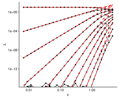
Figure 1: Eigenvalues of the Gaussian kernel ($d=1$). The set of $n=10$ nodes was drawn uniformly from the unit interval. In black, eigenvalues of the Gaussian kernel, for different values of $\varepsilon$. The dashed red curve are our small-$\varepsilon$ expansions. Note that both axes are scaled logarithmically. The noise apparent for small $\varepsilon$ values in the low range is due to loss of precision in the numerical computations.

Contrast that behaviour with the one exhibited by the eigenvalues of the exponential kernel. Theorem 4.7 describes the expected behaviour: the top eigenvalue is again $\mathcal{O}(1)$ and goes to $n$, while all remaining eigenvalues are $\mathcal{O}(\varepsilon)$. Fig. 2 is the counterpart of the previous figure, and shows clearly that all eigenvalues except for the top one go to 0 at unit rate. The main term in the expansions of eigenvalues determines again the offsets shown in Fig. 2, which can be computed from the eigenvalues of the centred distance matrix as shown in Theorem 4.7.

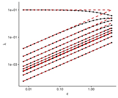
Figure 2: Eigenvalues of the exponential kernel ($d=1$), using the same set of points as in Fig. 1. The largest eigenvalue has a slope of 0 for small $\varepsilon$, the others have unit slope, as in Theorem 4.6.

To sum up: except for the top eigenvalue, which behaves in the same way for both kernels, the rest scale quite differently. More generally, Theorem 4.7 states that for kernels of smoothness order $r<n$ ($r=1$ for the exponential, $r=\infty$ for the Gaussian), the eigenvalues are divided into two groups. The first group of eigenvalues is of size $r$, and have orders $1$, $\varepsilon^{2}$, $\varepsilon^{4}$, etc. The second group is of size $n-r$, and all have the same order, $\varepsilon^{2r-1}$.

The difference between the two kernels is also reflected in how the eigenvectors behave. For the Gaussian kernel, the limiting eigenvectors (shown in Fig. 3) are columns of the $\bm{Q}$ matrix of the QR factorization of the Vandermonde matrix (i.e., the orthogonal polynomials with respect to the discrete uniform measure on $\mathcal{X}$). For instance, the top eigenvector equals the constant vector $\frac{1}{\sqrt{n}}\mathbf{1}$, and the second eigenvector equals $\begin{bmatrix}x_{1}&\cdots&x_{n}\end{bmatrix}^{{\sf T}}-\frac{\sum x_{i}}{n}$ (up to normalisation). Each successive eigenvector depends on the geometry of $\mathcal{X}$ via the moments $m_{p}(\mathcal{X})=\sum_{i=1}^{n}x^{p}_{i}$. In fact, this result is valid for any positive definite smooth analytic in $\varepsilon$ kernel as shown by Corollary 4.4.

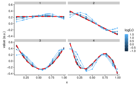
Figure 3: First four eigenvectors of the Gaussian kernel. We used the same set of points as in the previous two figures. In blue, eigenvectors of the Gaussian kernel, for different values of $\varepsilon$. The dashed red curve shows the theoretical limit as $\varepsilon\rightarrow 0$ (i.e., the first four orthogonal polynomials of the discrete measure)

In the case of finite smoothness, the two groups are associated with different groups of eigenvectors. The first group of $r$ eigenvectors are again orthogonal polynomials. The second group are splines of order $2r-1$. Convergence of eigenvectors is shown in Fig. 4. This general result for eigenvectors is shown in Theorem 8.1.

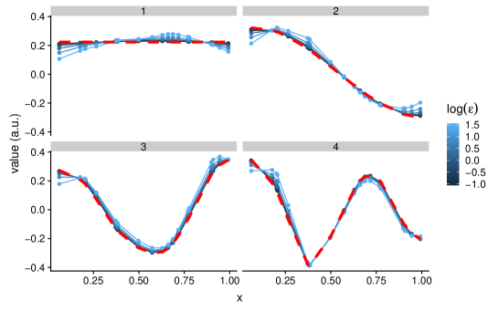
Figure 4: First four eigenvectors of the exponential kernel. The same set of nodes is used as in Fig. 3. In blue, the eigenvectors of the kernel, for different values of $\varepsilon$. The dashed red curve shows the theoretical limit as $\varepsilon\rightarrow 0$. From Theorem 8.1, these are (1) the vector $\frac{\mathbf{1}}{\sqrt{n}}$ and (2-4) the first three eigenvectors of $\left(\bm{I}-\frac{\mathbf{1}\mathbf{1}^{{\sf T}}}{n}\right)\bm{D}_{(1)}\left(\bm{I}-\frac{\mathbf{1}\mathbf{1}^{{\sf T}}}{n}\right)$, where $\bm{D}_{(1)}$ is the Euclidean distance matrix.

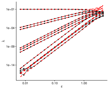
Figure 5: Eigenvalues of the Gaussian kernel in the multivariate case ($d=2$). The set of $n=10$ nodes was drawn uniformly from the unit square. In black, eigenvalues of the Gaussian kernel, for different values of $\varepsilon$. The dashed red curve are our small-$\varepsilon$ expansions. Eigenvalues appear in groups of different orders, recognisable here as having the same slopes as $\varepsilon\rightarrow 0$. A single eigenvalue is of order $\mathcal{O}(1)$. Two eigenvalues are of order $\mathcal{O}(\varepsilon^{2})$, as many as there are monomials of degree 1 in two dimensions. Three eigenvalues are of order $\mathcal{O}(\varepsilon^{4})$, as many as there are monomials of degree 2 in two dimensions, etc.

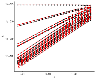
Figure 6: Eigenvalues of a finitely smooth kernel in $d=2$. Here we picked a kernel with smoothness index $r=3$ (the exponential kernel has order $r=1$). The set of $n=20$ nodes was drawn uniformly from the unit square. The first $r=3$ groups of eigenvalues have the same behaviour as in the Gaussian kernel: one is $\mathcal{O}(1)$, two are $\mathcal{O}(\varepsilon^{2})$, three are $\mathcal{O}(\varepsilon^{4})$. All the rest are $\mathcal{O}(\varepsilon^{5})$.

1.1.3 The multivariate case

The general, multivariate case requires more care. Polynomials continue to play a central role in the flat limit, but when $d>1$ they appear naturally in groups of equal degree. For instance, in $d=2$, we may write $\bm{x}=\left[\begin{smallmatrix}y&z\end{smallmatrix}\right]^{{\sf T}}$ and the first few monomials are as follows:

• Degree 0: $1$

• Degree 1: $y$, $z$

• Degree 2: $y^{2}$, $yz$, $z^{2}$

• Degree 3: $y^{3}$, $y^{2}z$, $yz^{2}$, $z^{3}$

etc. Note that there is one monomial of degree 0, two degree-$1$ monomials, three degree-$2$ monomials, and so on. If $d=1$ there is a single monomial in each group, and here lies the essence of the difference between the univariate and multivariate cases.

In infinitely smooth kernels like the Gaussian kernel, as shown in [31, 42], there are as many eigenvalues of order $\mathcal{O}(\varepsilon^{2k})$ as there are monomials of degree $k$ in dimension $d$: for instance, there are 4 monomials of degree 3 in dimension 2, and so 4 eigenvalues of order $\mathcal{O}(\varepsilon^{8})$. An example is shown on Fig. 5. In finitely-smooth kernels like the exponential kernel, there are $r$ successive groups of eigenvalues with order $\mathcal{O}(1)$, $\mathcal{O}(\varepsilon^{2})$, …, up to $\mathcal{O}(\varepsilon^{2r-2})$. Following that, all remaining eigenvalues have order $\mathcal{O}(\varepsilon^{2r-1})$, just like in the one-dimensional case.

We show in Theorem 6.2, that the main terms of these eigenvalues in each group can be computed from the QR factorization of the Vandermonde matrix and a Schur complement associated with the Wronskian matrix of the kernel. In the finite smoothness case, the same expansions are valid until the smoothness order, and the last group of eigenvalues is given by the eigenvalues of the projected distance matrix, as in the one-dimensional case.

Finally, in the multivariate case, Theorem 6.2 characterises the eigenprojectors. In a nutshell, the invariant subspaces associated with each group of eigenvalues are spanned by orthogonal polynomials of a certain order. The eigenvectors are the subject of a conjecture given in section 8, which we believe to be quite solid.

1.2 Overview of tools used in the paper

For finding the orders of the eigenvalues, as in [31, 42], we use the Courant-Fischer minimax principle (see Theorem 3.8). However, unlike [31, 42], we do not use directly the results of Micchelli [28], but rather rotate the kernel matrices using the $Q$ factor in the QR factorization of the Vandermonde matrix, and find the expansion of rotated matrices from the Taylor expansion of the kernel.

The key results are the expansions for the determinants of $\bm{K}_{\varepsilon}$, which use the expansions of rotated kernel matrices. Our results on determinants (Theorems 4.1, 4.6, 6.1, and 6.4) generalize those of Lee & Micchelli [26]. The next key observation is that principal submatrices of $\bm{K}_{\varepsilon}$ are also kernel matrices, hence the results on determinants imply the results on expansions elementary symmetric polynomials of eigenvalues (via the correspondence between elementary symmetric polynomials, see Theorem 3.1, and the Binet-Cauchy formula). Finally, the main terms of the eigenvalues can be retrieved from the main terms of the elementary symmetric polynomials, as shown in Lemma 3.3. An important tool for the multivariate and finite smoothness case is Lemma 3.15 on low-rank perturbation of elementary symmetric polynomials that we could not find elsewhere in the literature

To study the properties of the eigenvectors, we use analyticity of the eigenvalues and eigenprojectors for Hermitian analytic matrix-valued functions [22]. By using an extension of the Courant-Fischer principle (see Lemma 3.12), we can fully characterise the limiting eigenvectors in the univariate case, and obtain the limiting invariant subspaces for the groups of the limiting eigenvectors in the multivariate case. Moreover, by using the perturbation expansions from [22], we can find the last individual eigenvectors in the finitely smooth case.

We note that the multivariate case requires a number of technical assumptions on the arrangement of points, which are typical for multivariate polynomial interpolation. For the results on determinants, no assumptions are required. However, for getting the results on the eigenvalues or eigenvectors at a certain order of $\varepsilon$, we need a relaxed version to the well-known unisolvency condition [31, 14], namely the multivariate Vandermonde matrix up to the corresponding degree to be full rank.

1.3 Organisation of the paper

In an attempt to make the paper reader-friendly, it is organized as follows. In Section 2 we recall the main terminology for 1D kernels. In Section 3 we gather well-known (or not so well known) results on eigenvalues, determinants, elementary symmetric polynomials and their perturbations, which are key tools used in the paper. Section 4 contains the main results on determinants, eigenvalues, and eigenvectors in the univariate ($d=1$) case. While these results are special cases of the multivariate case ($d>1$), the latter is burdened with heavier notation due to the complexity of dealing with multivariate polynomials. To get a gist of the results and techniques, the reader is advised to first consult the case $d=1$. In Section 5, we introduce all the needed notation to handle the multivariate case. Section 6 contains the main results of the paper on determinants, eigenvalues, and groups of eigenvectors in the multivariate case. Thus Sections 2 to 6 are quite self-contained and contain most of the results in the paper, except the result on precise locations of the last group of eigenvectors in the finite smoothness case. In Section 7, we provide a brief summary on analytic perturbation theory, needed only for proving the stronger result on eigenvectors for finitely smooth kernels in Section 8.

2 Background and main notation

This section contains main definitions and examples of kernels, mostly in the 1D case (with multivariate extensions given in Section 5). We assume that the kernel $K:\Omega\times\Omega\to\mathbb{R}$ is in the class $\mathcal{C}^{(\ell,\ell)}(\Omega)$, $\Omega=(-a;a)$, i.e. all the partial derivatives $\frac{\partial^{2}}{\partial x^{i}\partial y^{j}}K$ exist and are continuous for $0\leq i,j\leq\ell$ on $\Omega\times\Omega$.

We will often need the following short-hand notation for partial derivatives

$$K^{(i,j)}\stackrel{{\scriptstyle\textrm{def}}}{{=}}\frac{\partial^{i+j}}{\partial x^{i}\partial y^{j}}K,$$

and we introduce the so-called Wronskian matrix

(4) $$\bm{W}_{\color[rgb]{0,0,0}\leq k\color[rgb]{0,0,0}}\stackrel{{\scriptstyle\textrm{def}}}{{=}}\begin{bmatrix}\frac{K^{(0,0)}(0,0)}{0!0!}&\cdots&\frac{K^{(0,k)}(0,0)}{0!k!}\\ \vdots&&\vdots\\ \frac{K^{(k,0)}(0,0)}{k!0!}&\cdots&\frac{K^{(k,k)}(0,0)}{k!k!}\end{bmatrix}.$$

2.1 Translation invariant and radial kernels

Let us consider an important example of a translation invariant (2) kernel, which in the univariate case becomes $K(x,y)=\varphi(x-y)$. We assume that $\varphi\in\mathcal{C}^{2r}(-2a,2a)$; hence, $\varphi$ has a Taylor expansion around $0$

$$\varphi(t)=\alpha_{0}+\alpha_{1}t+\alpha_{2}t^{2}+\cdots+\alpha_{2r}t^{2r}+o(t^{2r}),\quad\text{where}\;\alpha_{k}\stackrel{{\scriptstyle\textrm{def}}}{{=}}\frac{\varphi^{(k)}(0)}{k!}.$$

Therefore $K\in\mathcal{C}^{(r,r)}(\Omega\times\Omega)$ and its derivatives at $0$ are

(5) $$\frac{K^{(i,j)}(0,0)}{i!j!}=\frac{(-1)^{j}\varphi^{(i+j)}(0)}{i!j!}=(-1)^{j}{i+j\choose j}\alpha_{i+j},$$

i.e., the Wronskian matrix has the form:

$$\bm{W}_{\color[rgb]{0,0,0}\leq k\color[rgb]{0,0,0}}=\begin{bmatrix}\alpha_{0}&-\alpha_{1}&\alpha_{2}&-\alpha_{3}&\cdots\\ \alpha_{1}&-2\alpha_{2}&3\alpha_{3}&-4\alpha_{4}&\cdots\\ \alpha_{2}&-3\alpha_{3}&6\alpha_{4}&-10\alpha_{5}&\cdots\\ \alpha_{3}&-4\alpha_{4}&10\alpha_{5}&-20\alpha_{6}&\cdots\\ \vdots&\vdots&\vdots&\vdots&\ddots\\ \end{bmatrix}.$$

A special case of the translational kernels are smooth and radial, which will be considered in the next subsection. The simplest example is the Gaussian kernel with

$$\varphi(t)=\exp(-t^{2})=1-t^{2}+\frac{t^{4}}{2!}-\frac{t^{6}}{3!}+\cdots,$$

i.e. for all integer $\nu\geq 0$

$$\alpha_{2\nu}=\frac{(-1)^{\nu}}{\nu!},\quad\alpha_{2\nu+1}=0.$$

In this case, the Wronskian matrix becomes

$$\bm{W}_{\color[rgb]{0,0,0}\leq k\color[rgb]{0,0,0}}=\begin{bmatrix}1&0&-1&0&\cdots\\ 0&2&0&-2&\cdots\\ -1&0&3&0&\cdots\\ 0&-2&0&-\frac{10}{3}&\cdots\\ \vdots&\vdots&\vdots&\vdots&\ddots\\ \end{bmatrix}.$$

An important subclass consists of radial kernels (3), i.e., $K(x,y)=f(|x-y|)$ in the univariate case.

We put following the assumptions on $f$:

• $f\in\mathcal{C}^{2r}(-2a,2a)$;

• the highest derivative of odd order is not zero, i.e., $f^{(2r-1)}(0)\neq 0$;

• the lower derivatives with odd order vanish, i.e., $f^{(2\ell-1)}(0)=0$ for $\ell<r$.

If the function $f(t)$ satisfies these assumptions, then $r$ is called the order of smoothness of $K$. Note that $f$ admits a Taylor expansion

(6) $$f(t)=f_{0}+f_{2}t^{2}+\cdots+f_{2r-2}t^{2r-2}+t^{2r-1}(f_{2r-1}+\mathcal{O}(t)).$$

where $f_{k}=f^{(k)}(0)/k!$ is a shorthand notation for the scaled derivative at $0$. For example, for the exponential kernel $\exp(-|x-y|)$, we have $f_{0}=1$ and $f_{1}=-1$, so the smoothness order is $r=1$. For the $\mathcal{C}^{2}$ Matern kernel $(1+|x-y|)\exp(-|x-y|)$, we have $f_{0}=1,f_{1}=0,f_{2}=-1/2,f_{3}=1/3$, so the smoothness order is $r=2$.

2.2 Distance matrices, Vandermonde matrices, and their properties

In the general multivariate case, we define ${\bm{D}_{(k)}}$ to be the $k$-th Hadamard power of the Euclidean distance matrix $\bm{D}_{(1)}$, i.e.,

$$\bm{D}_{(k)}=\left[\left\|\bm{x}_{i}-\bm{x}_{j}\right\|_{2}^{k}\right]^{n,n}_{i,j=1}.$$

Next, we focus on the univariate case (the multivariate case will be discussed later in Section 5) and denote by $\bm{V}_{\leq k}$ the univariate Vandermonde matrix up to degree $k$

(7) $$\bm{V}_{\leq k}=\begin{bmatrix}1&x_{1}&\cdots&x^{k}_{1}\\ \vdots&\vdots&&\vdots\\ 1&x_{n}&\cdots&x^{k}_{n}\end{bmatrix},$$

which has rank $\min(n,k+1)$ if the nodes are distinct. In particular, the matrix $\bm{V}_{\leq n-1}$ is square and invertible for distinct nodes.

For even $k$, the Hadamard powers ${\bm{D}_{(k)}}$ of the distance matrix can be expressed via the columns of the Vandermonde matrix using the binomial expansion

(8) $${\bm{D}_{(2\ell)}}=\sum\limits_{j=0}^{2\ell}(-1)^{j}{2\ell\choose j}\bm{v}_{j}\bm{v}_{2\ell-j}^{{\sf T}},$$

where $\bm{v}_{k}\stackrel{{\scriptstyle\textrm{def}}}{{=}}\begin{bmatrix}x^{k}_{1}&\cdots&x^{k}_{n}\end{bmatrix}^{{\sf T}}$ are columns of Vandermonde matrices. Therefore, $\operatorname{rank}\bm{D}_{(2\ell)}=\min(2\ell+1,n)$ if all points $x_{k}$ are distinct.

On the other hand, for $k$ odd, the matrices $\bm{D}_{(k)}$ exhibit an entirely different set of properties. Of most interest here is conditional positive-definitess, which guarantees that the distance matrices are positive definite when projected on a certain subspace. The following result appears eg. in [12], ch. 8, but follows directly from an earlier paper by Micchelli [28].

Lemma 2.1.

For a distinct node set $\mathcal{X}\subset\mathbb{R}$ of size $n>r\geq 1$, we let $\bm{B}$ be a full column rank matrix such that $\bm{B}^{{\sf T}}\bm{V}_{\leq r-1}=0$. Then the matrix $(-1)^{r}\bm{B}^{{\sf T}}\bm{D}_{(2r-1)}\bm{B}$ is positive definite.

For instance, if $r=1$, we may pick any basis $\bm{B}$ orthogonal to the vector $\mathbf{1}$, and the lemma implies that $(-\bm{B}^{{\sf T}}\bm{D}_{(1)}\bm{B})$ has $n-1$ positive eigenvalues. We note for future reference that the result generalises almost unchanged to the multivariate case.

2.3 Scaling and expansions of kernel matrices

In this subsection, we consider the general multivariate case. Given a general kernel $K$, we define its scaled version as

(9) $$K_{\varepsilon}(\bm{x},\bm{y})=K(\varepsilon\bm{x},\varepsilon\bm{y}),$$

while for the specific case of radial kernels we use the following form

(10) $$K_{\varepsilon}(\bm{x},\bm{y})=f(\varepsilon\left\|\bm{x}-\bm{y}\right\|_{2}).$$

Note that the definitions (9) and (10) coincide for nonnegative $\varepsilon$, but differ if we formally take other values (e.g. complex) of $\varepsilon$. Depending on context, we will use one or the other of the definitions later on, especially when we talk about analyticity of kernel matrices.

Using (6) and (10), we may write the scaled kernel matrix (1), as

(11) $$\bm{K}_{\varepsilon}=f_{0}\bm{D}_{(0)}+\varepsilon^{2}f_{2}\bm{D}_{(2)}+\cdots+\varepsilon^{2r-2}f_{2r-2}\bm{D}_{(2r-2)}+\varepsilon^{2r-1}f_{2r-1}\bm{D}_{(2r-1)}+\mathcal{O}(\varepsilon^{2r}).$$

In the univariate case, (8) gives a way to rewrite the expansion (11) as

(12) $$\bm{K}_{\varepsilon}=\sum_{\ell=0}^{r-1}\varepsilon^{2j}\underbrace{\bm{V}_{\leq 2\ell}\bm{W}_{\diagup 2\ell}\bm{V}^{{\sf T}}_{\leq 2\ell}}_{f_{2\ell}\bm{D}_{(2\ell)}}+\varepsilon^{2r-1}f_{2r-1}\bm{D}_{(2r-1)}+\mathcal{O}(\varepsilon^{2r}),$$

where $\bm{W}_{\diagup s}\in\mathbb{R}^{(s+1)\times(s+1)}$ has nonzero elements only on its antidiagonal:

(13) $$\Big{(}\bm{W}_{\diagup s}\Big{)}_{i+1,s-i+1}\stackrel{{\scriptstyle\textrm{def}}}{{=}}f_{s}(-1)^{i}{s\choose i}.$$

For example,

$$\bm{W}_{\diagup 2}=f_{2}\begin{bmatrix}0&0&1\\ 0&-2&0\\ 1&0&0\end{bmatrix}.$$

In fact, from (5), non-zero elements of $\bm{W}_{\diagup s}$ are scaled derivatives of the kernel:

$$\Big{(}\bm{W}_{\diagup s}\Big{)}_{i+1,s-i+1}=\frac{K^{(i,s-i)}(0,0)}{i!(s-i)!};$$

this justifies the notation $\bm{W}_{\diagup s}$ (i.e., an antidiagonal of the Wronskian matrix).

3 Determinants and elementary symmetric polynomials

In this paper, we will heavily use the elementary symmetric polynomials of eigenvalues, and we collect in this section some useful (more or less known) facts about them.

3.1 Eigenvalues, principal minors and elementary symmetric polynomials

The $k$-th elementary symmetric polynomial of $\lambda_{1},\ldots,\lambda_{n}$ is defined as:

(14) $$e_{k}(\lambda_{1},\ldots,\lambda_{n})=\sum_{\begin{subarray}{c}\color[rgb]{0,0,0}\#\mathcal{Y}\color[rgb]{0,0,0}=k\\ \mathcal{Y}\subset\{1,\ldots,n\}\end{subarray}}\,\prod_{i\in\mathcal{Y}}\lambda_{i},$$

i.e., the sum is running over all possible subsets of $\{1,\ldots,n\}$ of size $k$. In particular, $e_{1}(\lambda_{1},\ldots,\lambda_{n})=\sum_{i=1}^{n}\lambda_{i}$, $e_{2}(\lambda_{1},\ldots,\lambda_{n})=\sum_{i<j}\lambda_{i}\lambda_{j}$, and $e_{n}(\lambda_{1},\ldots,\lambda_{n})=\prod_{i=1}^{n}\lambda_{i}$.

Next, we consider the elementary symmetric polynomials (ESPs) applied to eigenvalues of matrices, and define (with some abuse of notation):

$$e_{k}(\bm{A})\stackrel{{\scriptstyle\textrm{def}}}{{=}}e_{k}(\lambda_{1}(\bm{A}),\ldots,\lambda_{n}(\bm{A})).$$

Then the first and the last polynomials are the trace and determinant of $\bm{A}$:

$$e_{1}(\bm{A})=\operatorname{Tr}\bm{A},\quad e_{n}(\bm{A})=\det\bm{A}.$$

This fact is a special case of a more general result on sums of principal minors.

Theorem 3.1 ([19, Theorem 1.2.12]).

(15) $$e_{k}(\bm{A})=\sum_{\begin{subarray}{c}\mathcal{Y}\subset\{1,\ldots,n\}\\ \color[rgb]{0,0,0}\#\mathcal{Y}\color[rgb]{0,0,0}=k\end{subarray}}\det(\bm{A}_{\mathcal{Y},\mathcal{Y}})$$

where $\bm{A}_{\mathcal{Y},\mathcal{Y}}$ is a submatrix of $\bm{A}$ with rows and columns indexed by $\mathcal{Y}$, i.e. the sum runs over all principal minors of size $k\times k$.

Remark 3.2.

The scaled symmetric polynomials $(-1)^{k}e_{k}(\bm{A})$ are the coefficients of the characteristic polynomial $\det(\lambda\bm{I}-\bm{A})$ at the coefficient $\lambda^{n-k}$.

3.2 Orders of elementary symmetric polynomials

Next, we assume that $\lambda_{1}(\varepsilon),\ldots,\lambda_{n}(\varepsilon)$ are functions of some small parameter $\varepsilon$ and we are interested in the orders of the corresponding elementary symmetric polynomials

$$e_{s}(\varepsilon)\stackrel{{\scriptstyle\textrm{def}}}{{=}}e_{s}(\lambda_{1}(\varepsilon),\ldots,\lambda_{n}(\varepsilon)),\quad 1\leq s\leq n,$$

as $\varepsilon\to 0$. The following obvious observation will be important.

Lemma 3.3.

Assume that

$$\lambda_{1}(\varepsilon)=\mathcal{O}(\varepsilon^{L_{1}}),\;\lambda_{2}(\varepsilon)=\mathcal{O}(\varepsilon^{L_{2}}),\;\ldots,\;\lambda_{n}(\varepsilon)=\mathcal{O}(\varepsilon^{L_{n}}),$$

as $\varepsilon\to 0$ and $0\leq L_{1}\leq\cdots\leq L_{n}$ are some integers. Then it holds that

$$e_{1}(\varepsilon)=\mathcal{O}(\varepsilon^{L_{1}}),\;e_{2}(\varepsilon)=\mathcal{O}(\varepsilon^{L_{1}+L_{2}}),\;\ldots,\;e_{n}(\varepsilon)=\mathcal{O}(\varepsilon^{L_{1}+\cdots+L_{n}}).$$

Proof 3.4.

The proof follows from the definition of $e_{s}$ the fact that the product $f(\varepsilon)=\mathcal{O}(\varepsilon^{a})$ and $g(\varepsilon)=\mathcal{O}(\varepsilon^{b})$ is of the order$f(\varepsilon)g(\varepsilon)=\mathcal{O}(\varepsilon^{a+b})$.

We will need a refinement of Lemma 3.3 concerning the main terms of such functions. We distinguish two situations: when the orders of $\lambda_{k}$ are separated, and when they form groups. For example, if $\lambda_{1}(\varepsilon)=a+\mathcal{O}(\varepsilon)$, $\lambda_{2}(\varepsilon)=\varepsilon(b+\mathcal{O}(\varepsilon))$, $\lambda_{3}(\varepsilon)=\varepsilon^{2}(c+\mathcal{O}(\varepsilon))$, then the main terms of ESPs are products of the main terms of $\lambda_{k}$

$$e_{1}(\varepsilon)=a+\mathcal{O}(\varepsilon),\quad e_{2}(\varepsilon)=\varepsilon(ab+\mathcal{O}(\varepsilon)),\quad e_{3}(\varepsilon)=\varepsilon^{3}(abc+\mathcal{O}(\varepsilon)).$$

On the other hand, in case $\lambda_{1}(\varepsilon)=a+\mathcal{O}(\varepsilon)$, $\lambda_{k+1}(\varepsilon)=\varepsilon(b_{k}+\mathcal{O}(\varepsilon))$, $k\in\{1,2,3\}$, the behaviour of main terms of ESPs is different:

$$e_{1}(\varepsilon) =a+\mathcal{O}(\varepsilon),\quad e_{2}(\varepsilon)=\varepsilon(a(b_{1}+b_{2}+b_{3})+\mathcal{O}(\varepsilon)),$$

$$e_{3}(\varepsilon) =\varepsilon^{2}(a(b_{1}b_{2}+b_{1}b_{3}+b_{2}b_{3})+\mathcal{O}(\varepsilon)),\quad e_{4}(\varepsilon)=\varepsilon^{3}(ab_{1}b_{2}b_{3}+\mathcal{O}(\varepsilon)).$$

The following two lemmas generalize these observations to arbitrary orders.

Lemma 3.5.

Suppose that $\lambda_{1}(\varepsilon),\ldots,\lambda_{n}(\varepsilon)$ have the form

(16) $$\lambda_{1}(\varepsilon)=\varepsilon^{L_{1}}(\widetilde{\lambda}_{1}+\mathcal{O}(\varepsilon)),\ldots\ ,\lambda_{n}(\varepsilon)=\varepsilon^{L_{n}}(\widetilde{\lambda}_{n}+\mathcal{O}(\varepsilon)),$$

for some integers $0\leq L_{1}\leq\cdots\leq L_{r}$. Then

1. The elementary symmetric polynomials have the form

   (17) $$\begin{split}e_{1}(\varepsilon)&=\varepsilon^{L_{1}}(\widetilde{e}_{1}+\mathcal{O}(\varepsilon))\\ e_{2}(\varepsilon)&=\varepsilon^{L_{1}+L_{2}}(\widetilde{e}_{2}+\mathcal{O}(\varepsilon))\\ \vdots\\ e_{n}(\varepsilon)&=\varepsilon^{L_{1}+\cdots+L_{n}}(\widetilde{e}_{n}+\mathcal{O}(\varepsilon)).\end{split}$$

2. If either $s=n$ or $L_{s}<L_{s+1}$, the main term $\widetilde{e}_{s}$ can be expressed as

   $$\widetilde{e}_{s}=\widetilde{\lambda}_{1}\cdots\widetilde{\lambda}_{s}.$$

   In particular, if $s>1$ and $\widetilde{e}_{s-1}\neq 0$, then the main term $\widetilde{\lambda}_{s}$ can be found as

   $$\widetilde{\lambda}_{s}=\frac{\widetilde{e}_{s}}{\widetilde{e}_{s-1}}.$$

We also need a generalization of Lemma 3.5 to the case of a group of equal $L_{k}$.

Lemma 3.6.

Let $\lambda_{k}(\varepsilon)$ and $L_{k}$ be as in Lemma 3.5 (i.e., $\lambda_{k}(\varepsilon)$ have the form (16) and the corresponding $e_{k}(\varepsilon)$ have the form (17)), and define $L_{0}=-1$, $L_{n+1}=+\infty$, for an easier treatment of border cases.

If for $\color[rgb]{0,0,0}1\color[rgb]{0,0,0}\leq m\leq n-s$, there is a separated group of $m$ functions

$$\lambda_{s+1}(\varepsilon),\ldots,\lambda_{s+m}(\varepsilon)$$

of repeating degree, i.e.

(18) $$L_{s}<L_{s+1}=\cdots=L_{s+m}<L_{s+m+1},$$

then the main terms $\widetilde{e}_{s+k}$, $1\leq k\leq m$ in (17), are connected with ESPs of the main terms $\widetilde{\lambda}_{s+k}$, $1\leq k\leq m$ as follows:

$$\widetilde{e}_{s+k}=\begin{cases}e_{k}(\widetilde{\lambda}_{s+1},\ldots,\widetilde{\lambda}_{s+m}),&s=0,\\ \widetilde{\lambda}_{1}\cdots\widetilde{\lambda}_{s}e_{k}(\widetilde{\lambda}_{s+1},\ldots,\widetilde{\lambda}_{s+m})=\widetilde{e}_{s}e_{k}(\widetilde{\lambda}_{s+1},\ldots,\widetilde{\lambda}_{s+m}),&s>0.\end{cases}$$

In particular, if $s>1$ and $\widetilde{e}_{s}\neq 0$, the ESPs for the main terms are equal to

$$e_{k}(\widetilde{\lambda}_{s+1},\ldots,\widetilde{\lambda}_{s+m})=\frac{\widetilde{e}_{s+k}}{\widetilde{e}_{s}},$$

hence $\widetilde{\lambda}_{s+1},\ldots,\widetilde{\lambda}_{s+m}$ are the roots of the polynomial (see Remark 3.2)

$$q(\lambda)=\widetilde{e}_{s}\lambda^{m}-\widetilde{e}_{s+1}\lambda^{m-1}+\widetilde{e}_{s+2}\lambda^{m-2}+\cdots+(-1)^{m}\widetilde{e}_{s+m}.$$

Proofs of Lemmas 3.5 to 3.6 are contained in Appendix A. Note that for analytic $\lambda_{k}(\varepsilon)$, Lemma 3.5 and Lemma 3.6 follow from the Newton-Puiseux theorem (see, for example, [36, §2.1]), but we prefer to keep a more general formulation in this paper.

Remark 3.7.

Assumptions in Lemmas 3.5 to 3.6 can be relaxed (when expansions (16) are valid up to a certain order), but we keep the current statement for simplicity.

3.3 Orders of eigenvalues and eigenvectors

First, we recall a corollary of the Courant-Fischer “min-max” principle giving a bound on smallest eigenvalues.

Theorem 3.8 ([19, Theorem 4.3.21]).

Let $\bm{A}\in\mathbb{R}^{n\times n}$ be symmetric, and its eigenvalues arranged in non-increasing order $\lambda_{1}\geq\lambda_{2}\geq\cdots\geq\lambda_{n}$. If there exist an $m$-dimensional subspace $\mathcal{L}\subset\mathbb{R}^{n}$ and a constant $c_{1}$ such that

$$\frac{\bm{u}^{{\sf T}}\bm{A}\bm{u}}{\bm{u}^{{\sf T}}\bm{u}}\leq c_{1},$$

for all $\bm{u}\in\mathcal{L}\setminus\{\bm{0}\}$, then the smallest $m$ eigenvalues are bounded as

$$\lambda_{n}\leq\lambda_{n-1}\leq\cdots\leq\lambda_{n-m+1}\leq c_{1}.$$

For determining the orders of eigenvalues, we will need the following corollary of Theorem 3.8 (see the proof of [42, Theorem 8]). We provide a short proof for completeness.

Lemma 3.9.

Suppose that $\bm{K}(\varepsilon)\in\mathbb{R}^{n\times n}$ is symmetric positive semidefinite for $\varepsilon\in[0,\varepsilon_{0}]$ and its eigenvalues are ordered as

$$\lambda_{1}(\varepsilon)\geq\lambda_{2}(\varepsilon)\geq\cdots\geq\lambda_{n}(\varepsilon)\geq 0.$$

Suppose that there exists a matrix $\bm{U}\in\mathbb{R}^{n\times m}$, $\bm{U}^{{\sf T}}\bm{U}=\bm{I}_{m}$, such that

(19) $$\bm{U}^{{\sf T}}\bm{K}(\varepsilon)\bm{U}=\mathcal{O}(\varepsilon^{L})$$

in $[0,\varepsilon_{0}]$, $\varepsilon_{0}>0$. Then the last $m$ eigenvalues of $\bm{K}(\varepsilon)$ are of order at least $L$, i.e.,

(20) $$\lambda_{j}(\varepsilon)=\mathcal{O}(\varepsilon^{L}),\text{ for }n-m<j\leq n.$$

Proof 3.10.

Assumption (19) and equivalence of matrix norms implies that

$$\|\bm{U}^{{\sf T}}\bm{K}(\varepsilon)\bm{U}\|_{2}\leq C\varepsilon^{L}.$$

for some constant ${C}$. Hence, we have that for any $\bm{z}\in\mathbb{R}^{m}\setminus\{0\}$,

$$\frac{\bm{z}^{{\sf T}}\bm{U}^{{\sf T}}\bm{K}(\varepsilon)\bm{U}\bm{z}}{\bm{z}^{{\sf T}}\bm{U}^{{\sf T}}\bm{U}\bm{z}}\leq\|\bm{U}^{{\sf T}}\bm{K}(\varepsilon)\bm{U}\|_{2}\leq C\varepsilon^{L}.$$

By choosing the range of $\bm{U}$ as $\mathcal{L}$ and applying Theorem 3.8, we complete the proof.

Next, we recall a classic result on eigenvalues/eigenvectors for analytic perturbations.

Theorem 3.11 ([22, Ch. II, Theorem 1.10]).

Let $\bm{K}(\varepsilon)$ be an $n\times n$ matrix depending analytically on $\varepsilon$ in the neighborhood of $0$ and symmetric for real $\varepsilon$. Then all the eigenvalues $\lambda_{k}(\varepsilon)$, $1\leq k\leq n$ can be chosen analytic; moreover, the orthogonal projectors $\bm{P}_{k}(\varepsilon)$ on the corresponding rank-one eigenspaces can be also chosen analytic, so that

(21) $$\bm{K}(\varepsilon)=\sum_{k=1}^{n}\lambda_{k}(\varepsilon)\bm{P}_{k}(\varepsilon)$$

is the eigenvalue decomposition of $\bm{K}(\varepsilon)$ in a neighborhood of $0$.

We will be interested in finding the limiting rank-one projectors in Theorem 3.11 i.e.,

$$\bm{P}_{k}=\lim_{\varepsilon\to 0}\bm{P}_{k}(\varepsilon)=\bm{P}_{k}(0),$$

where the last equality follows from analyticity of $\bm{P}_{k}(\varepsilon)$ at $0$. Note that, for kernel matrices, it is impossible to retrieve the information about the limiting projectors just from $\bm{K}(0)$ (which is rank-one). In what follows, instead of $\bm{P}_{k}$ we will talk about limiting eigenvectors $\bm{p}_{k}$ (i.e., $\bm{P}_{k}=\bm{p}_{k}\bm{p}_{k}^{{\sf T}}$), although the latter are defined only up to a change of sign.

Armed with Theorem 3.11, we can obtain an extension of Lemma 3.9, which also gives us information about limiting eigenvectors.

Lemma 3.12.

Let $\bm{K}(\varepsilon)$ and $\bm{U}\in\mathbb{R}^{n\times m}$ be as in Lemma 3.9, and, moreover, $\bm{K}(\varepsilon)$ be analytic in the neighborhood of $0$.

Then $\operatorname{span}(\bm{U})$ contains all the limiting eigenvectors corresponding to the eigenvalues of the order at least $L$ (i.e., $\mathcal{O}(\varepsilon^{L})$).

Proof 3.13.

Let $L_{1}\leq\cdots\leq L_{k}\leq+\infty$ be the exact orders of the eigenvalues, i.e., either

$$\lambda_{k}(\varepsilon)=\varepsilon^{L_{k}}(\widetilde{\lambda}_{k}+\mathcal{O}(\varepsilon)),\quad\widetilde{\lambda}_{k}>0,$$

or $L_{k}=+\infty$ in case $\lambda_{k}(\varepsilon)\equiv 0$. Then, from orthogonality of the eigenvectors, we only need to prove that, $\bm{p}_{k}^{{\sf T}}\bm{U}=0$ for $L_{k}<L$. Note that $\widetilde{\lambda}_{k}>0$ due to positive semidefiniteness of $\bm{K}(\varepsilon)$.

Suppose that, on the contrary, there exists $k$ with $L_{k}<L$ such that $\bm{p}_{k}^{{\sf T}}\bm{U}\neq 0$, and let it be the minimal such $k$. Then from the factorization (21) we have that

$$\bm{U}^{{\sf T}}\bm{K}(\varepsilon)\bm{U}=\varepsilon^{L_{k}}\Big{(}{\sum\limits_{\ell:L_{\ell}=L_{k}}\widetilde{\lambda}_{\ell}\bm{U}^{{\sf T}}\bm{p}_{k}\bm{p}_{k}^{{\sf T}}\bm{U}}+\mathcal{O}(\varepsilon)\Big{)},$$

with a nonzero main term (from $\widetilde{\lambda}_{k}>0$), which contradicts the assumption (19).

3.4 Saddle point matrices and elementary symmetric polynomials

In this subsection, we will be interested in determinants and elementary symmetric polynomials for so-called saddle point matrices [4]. Let $\bm{V}\in\mathbb{R}^{n\times r}$ be a full column rank matrix. For a matrix $\bm{A}\in\mathbb{R}^{n\times n}$, we define the saddle-point matrix as

$$\begin{bmatrix}\bm{A}&\bm{V}\\ \bm{V}^{{\sf T}}&0\end{bmatrix}.$$

Consider a full QR decomposition of $\bm{V}\in\mathbb{R}^{n\times r}$, i.e.,

(22) $$\bm{V}=\color[rgb]{0,0,0}\bm{Q}_{\rm full}\color[rgb]{0,0,0}\color[rgb]{0,0,0}\bm{R}_{\rm full}\color[rgb]{0,0,0}=\color[rgb]{0,0,0}\bm{Q}\color[rgb]{0,0,0}\color[rgb]{0,0,0}\bm{R}\color[rgb]{0,0,0},\quad\color[rgb]{0,0,0}\bm{Q}_{\rm full}\color[rgb]{0,0,0}=\begin{bmatrix}\color[rgb]{0,0,0}\bm{Q}\color[rgb]{0,0,0}&\bm{Q}_{\bot}\end{bmatrix},\quad\color[rgb]{0,0,0}\bm{R}_{\rm full}\color[rgb]{0,0,0}=\begin{bmatrix}\color[rgb]{0,0,0}\bm{R}\color[rgb]{0,0,0}\\ \bm{0}\end{bmatrix},$$

where $\color[rgb]{0,0,0}\bm{Q}_{\rm full}\color[rgb]{0,0,0}\in\mathbb{R}^{n\times n}$, $\bm{Q}_{\bot}\in\mathbb{R}^{n\times(n\text{-}r)}$, $\color[rgb]{0,0,0}\bm{Q}_{\rm full}^{{\sf T}}\color[rgb]{0,0,0}\color[rgb]{0,0,0}\bm{Q}_{\rm full}\color[rgb]{0,0,0}=\bm{I}$, $\color[rgb]{0,0,0}\bm{R}\color[rgb]{0,0,0}$ is upper-triangular, and $\bm{Q}_{\bot}^{{\sf T}}\bm{V}=0$.

Lemma 3.14.

For any $\bm{A}\in\mathbb{R}^{n\times n}$ and $\bm{V}\in\mathbb{R}^{n\times r}$, it holds that

$$\det\begin{bmatrix}\bm{A}&\bm{V}\\ \bm{V}^{{\sf T}}&0\end{bmatrix}=(-1)^{r}\det(\bm{V}^{{\sf T}}\bm{V})\det(\bm{Q}_{\bot}^{{\sf T}}\bm{A}\bm{Q}_{\bot})=(-1)^{r}(\det\color[rgb]{0,0,0}\bm{R}\color[rgb]{0,0,0})^{2}\det(\bm{Q}_{\bot}^{{\sf T}}\bm{A}\bm{Q}_{\bot}),$$

where the matrices $\color[rgb]{0,0,0}\bm{R}\color[rgb]{0,0,0}$ and $\bm{Q}_{\bot}$ are from the full QR factorization given in (22). The proof of Lemma 3.14 is contained in Appendix B.

We will also also need to evaluate the elementary symmetric polynomials of matrices of the form $\bm{Q}_{\bot}^{{\sf T}}\bm{A}\bm{Q}_{\bot}$. For a power series (or a polynomial)

$$a(t)=a_{0}+a_{1}t+\cdots+a_{N}t^{N}+\ldots,$$

we use the following notation, standard in combinatorics, for its coefficients:

$$[t^{r}]\left\{a(t)\right\}\stackrel{{\scriptstyle\textrm{def}}}{{=}}a_{r}=\color[rgb]{0,0,0}\frac{a^{(r)}(0)}{r!}.\color[rgb]{0,0,0}$$

With this notation, the following lemma on low-rank perturbations of $\bm{A}$ holds true.

Lemma 3.15.

Let $\bm{A}\in\mathbb{R}^{n\times n}$ and $\bm{V}\in\mathbb{R}^{n\times r}$, with the QR decomposition of $\bm{V}$ given as before by eq. (22). Then for $k\geq r$ the polynomial $a(t)=e_{k}(\bm{A}+t\bm{V}\bm{V}^{{\sf T}})$ has degree at most $r$, and its leading coefficient is given by

$$[t^{r}]\left\{e_{k}(\bm{A}+t\bm{V}\bm{V}^{{\sf T}})\right\}=\det(\bm{V}^{{\sf T}}\bm{V})e_{k-r}(\bm{Q}_{\bot}^{{\sf T}}\bm{A}\bm{Q}_{\bot});$$

In particular, if $k=n$, we get

$$[t^{r}]\left\{\det(\bm{A}+t\bm{V}\bm{V}^{{\sf T}})\right\}=\det(\bm{V}^{{\sf T}}\bm{V})\det(\bm{Q}_{\bot}^{{\sf T}}\bm{A}\bm{Q}_{\bot})=(-1)^{r}\det\begin{bmatrix}\bm{A}&\bm{V}\\ \bm{V}^{{\sf T}}&0\end{bmatrix}.$$

The proof of Lemma 3.15 is also contained in Appendix B.

Remark 3.16.

Alternative expressions for perturbations of elementary symmetric polynomials are available in [20, Theorem 2.16], and [21, Corollary 3.3], but they do not lead directly to the compact expression in Lemma 3.15 that we need.

4 Results in the 1D case

4.1 Smooth kernels

We begin this section by generalizing the result of [26, Corollary 2.9] on determinants of scaled kernel matrix $\bm{K}_{\varepsilon}$ in the smooth case.

Theorem 4.1.

Let $K\in\mathcal{C}^{(n,n)}(\Omega\times\Omega)$ be the kernel, and (9) be its scaled version. Then for small $\varepsilon$,

1. the determinant of $\bm{K}_{\varepsilon}$ from (1) has the expansion

   $$\det(\bm{K}_{\varepsilon})=\varepsilon^{n(n-1)}(\det(\bm{V}_{\leq n-1})^{2}\det\bm{W}_{\color[rgb]{0,0,0}\leq n-1\color[rgb]{0,0,0}}+\mathcal{O}(\varepsilon)).$$

2. if $\bm{K}_{\varepsilon}$ is positive semidefinite on $[0,\varepsilon_{0}],\varepsilon_{0}>0,$ then eigenvalues have orders

   $${\lambda}_{k}(\varepsilon)=\mathcal{O}(\varepsilon^{2(k-1)}).$$

While the proof of 1) is given in [26, Corollary 2.9], and the proof of 2) for the radial analytic kernels is contained in [31, 42], we provide a short proof of Theorem 4.1 in Section 4.3, which also illustrates the main ideas behind other proofs in the paper.

Theorem 4.1, together with Theorem 3.1 allows us to find the main terms of the eigenvalues for analytic-in-parameter $\bm{K}_{\varepsilon}$.

Theorem 4.2.

Let $K\in\mathcal{C}^{(n,n)}(\Omega)$ be the kernel such that $\bm{K}_{\varepsilon}$ symmetric positive semidefinite on $[0,\varepsilon_{0}],\varepsilon_{0}>0,$ and analytic in $\varepsilon$ in the neighborhood of $0$. Then for $s\leq n$ it holds that

$${\lambda}_{s}=\varepsilon^{2(s-1)}(\widetilde{\lambda}_{s}+\mathcal{O}(\varepsilon)),$$

where the main terms satisfy

(23) $$\widetilde{\lambda}_{1}\ldots\widetilde{\lambda}_{s}=\det(\bm{V}^{{\sf T}}_{\leq s-1}\bm{V}_{\leq s-1})\det(\bm{W}_{\color[rgb]{0,0,0}\leq s-1\color[rgb]{0,0,0}}).$$

Proof 4.3.

First, due to analyticity and Theorem 4.1, we have that expansions (16) are valid for $L_{s}=2(s-1)$. Second, the submatrices of $\bm{K}_{\varepsilon}$ are also kernel matrices (of smaller size), which, in turn can be found from Theorem 4.1. More precisely,

$$e_{s}(\bm{K}_{\varepsilon}) =\sum\limits_{1\leq k_{1}<\cdots<k_{s}\leq n}\det(\bm{K}_{\varepsilon}({x_{k_{1}},\ldots,x_{k_{s}}}))$$

$$=\varepsilon^{s(s-1)}\Big{(}\det\bm{W}_{\color[rgb]{0,0,0}\leq s-1\color[rgb]{0,0,0}}\sum\limits_{1\leq k_{1}<\cdots<k_{s}\leq n}(\det\bm{V}_{\leq s-1}({x_{k_{1}},\ldots,x_{k_{s}}}))^{2}+\mathcal{O}(\varepsilon)\Big{)}$$

(24) $$=\varepsilon^{s(s-1)}\left(\det\bm{W}_{\color[rgb]{0,0,0}\leq s-1\color[rgb]{0,0,0}}\det(\bm{V}_{\leq s-1}^{{\sf T}}\bm{V}_{\leq s-1})+\mathcal{O}(\varepsilon)\right),$$

where the penultimate equality follows from Theorem 4.1, and the last equality follows from the Binet-Cauchy formula.

Finally, we employ Lemma 3.5 on relations between the main terms in (16) and (17).

Corollary 4.4.

Let $\bm{K}_{\varepsilon}$ be as in Theorem 4.2, and the points in $\mathcal{X}$ be distinct.

1. If for $1<s\leq n$, $\det\bm{W}_{\color[rgb]{0,0,0}\leq s-2\color[rgb]{0,0,0}}\neq 0$, the main term of the $s$-th eigenvalue can be obtained as

   (25) $$\widetilde{\lambda}_{s}=\frac{\det(\bm{V}^{{\sf T}}_{\leq s-1}\bm{V}_{\leq s-1})}{\det(\bm{V}^{{\sf T}}_{\leq s-2}\bm{V}_{\leq s-2})}\cdot\frac{\det(\bm{W}_{\color[rgb]{0,0,0}\leq s-1\color[rgb]{0,0,0}})}{\det(\bm{W}_{\color[rgb]{0,0,0}\leq s-2\color[rgb]{0,0,0}})}.$$

2. If $1\leq s<n$, $\det\bm{W}_{\color[rgb]{0,0,0}\leq s-1\color[rgb]{0,0,0}}\neq 0$, then the limiting eigenvectors $\bm{p}_{1},\ldots,\bm{p}_{s}$ are the first $s$ columns of the $\color[rgb]{0,0,0}\bm{Q}_{\rm full}\color[rgb]{0,0,0}$ factor of the QR factorization (22) of $\bm{V}_{\leq s-1}$.

3. In particular, if $\det\bm{W}_{\color[rgb]{0,0,0}\leq n-2\color[rgb]{0,0,0}}\neq 0$, then all the main terms of the eigenvalues are given by (25), and all the limiting eigenvectors are given by the columns of the $\bm{Q}$ matrix in the QR factorization of $\bm{V}_{\leq n-1}$.

The proof of Corollary 4.4 is also contained in Section 4.3.

Remark 4.5.

In Corollary 4.4, by Cramer’s rule, the individual ratios in (25) can be computed in the following way:

$$\frac{\det(\bm{V}^{{\sf T}}_{\leq s-1}\bm{V}_{\leq s-1})}{\det(\bm{V}^{{\sf T}}_{\leq s-2}\bm{V}_{\leq s-2})}=((\bm{V}^{{\sf T}}_{\leq s-1}\bm{V}_{\leq s-1})^{-1})^{-1}_{s,s}=R^{2}_{s,s},$$

where $R_{s,s}$ is the last ($(s,s)$-th) diagonal element of the $\color[rgb]{0,0,0}\bm{R}\color[rgb]{0,0,0}\in\mathbb{R}^{s\times s}$ matrix in the thin QR decomposition of $\bm{V}_{\leq s-1}$. Similarly,

$$\frac{\det(\bm{W}_{\color[rgb]{0,0,0}\leq s-1\color[rgb]{0,0,0}})}{\det(\bm{W}_{\color[rgb]{0,0,0}\leq s-2\color[rgb]{0,0,0}})}=((\bm{W}_{\color[rgb]{0,0,0}\leq s-1\color[rgb]{0,0,0}})^{-1})^{-1}_{s,s}=C^{2}_{s,s},$$

where $C_{s,s}$ is the last diagonal element of the Cholesky factor of $\bm{W}_{\color[rgb]{0,0,0}\leq s-1\color[rgb]{0,0,0}}=\bm{C}\bm{C}^{{\sf T}}$.

4.2 Finite smoothness

Next, we provide an analogue of Theorem 4.1 for a radial kernel with the order of smoothness $r$, which is smaller or equal to the number of points (i.e., Theorem 4.1 cannot be applied.).

Theorem 4.6.

For a radial kernel (10) with order of smoothness $r\leq n$,

1. the determinant can be expressed as

   $$\det(\bm{K}_{\varepsilon})=\varepsilon^{n(2r-1)-r^{2}}\left(\widetilde{k}+\mathcal{O}(\varepsilon)\right),$$

   where the main term is given by

   (26) $$\widetilde{k} =(-1)^{r}\det\bm{W}_{\color[rgb]{0,0,0}\leq r-1\color[rgb]{0,0,0}}\det\begin{bmatrix}f_{2r-1}\bm{D}_{(2r-1)}&\bm{V}_{\leq r-1}\\ \bm{V}_{\leq r-1}^{{\sf T}}&0\end{bmatrix}$$

   (27) $$=\det\bm{W}_{\color[rgb]{0,0,0}\leq r-1\color[rgb]{0,0,0}}\det(\bm{V}^{{\sf T}}_{\leq r-1}\bm{V}_{\leq r-1})\det(f_{2r-1}\bm{Q}_{\bot}^{{\sf T}}\bm{D}_{(2r-1)}\bm{Q}_{\bot}),$$

   where $\bm{Q}_{\bot}\in\mathbb{R}^{n\times(n-r)}$ is the semi-orthogonal matrix such that $\bm{Q}_{\bot}^{{\sf T}}\bm{V}_{\leq r-1}=0$ (e.g., the matrix $\bm{Q}_{\bot}$ in the full QR decomposition (22) of $\bm{V}=\bm{V}_{\leq r-1}$).

2. If $\bm{K}_{\varepsilon}$ is positive semidefinite on $[0,\varepsilon_{0}],\varepsilon_{0}>0,$ the eigenvalues have orders

   $${\lambda}_{s}(\varepsilon)=\begin{cases}\mathcal{O}(\varepsilon^{2(s-1)}),&s\leq r,\\ \mathcal{O}(\varepsilon^{2r-1}),&s>r.\\ \end{cases}$$

The proof of Theorem 4.6 again is postponed to Section 4.4 in order to present a more straightforward corollary on eigenvalues.

As an example, we have for $r=1$ (exponential kernel):

(28) $$\det(\bm{K}_{\varepsilon})=-\varepsilon^{n-1}nK(0,0)\det\begin{bmatrix}\bm{D}_{(1)}&\mathbf{1}\\ \mathbf{1}^{{\sf T}}&0\end{bmatrix},$$

where $\mathbf{1}$ denotes a vector with all entries equal to $1$.

Combining Theorem 4.6 with Lemmas 3.6 and 3.12, we get the following result.

Theorem 4.7.

Let $K$ be a kernel satisfying the assumptions of Theorem 4.6, where $\bm{K}_{\varepsilon}$ is positive semidefinite on $[0,\varepsilon_{0}],\varepsilon_{0}>0,$ and analytic in $\varepsilon$. Then it holds that

1. The main terms of first $r$ eigenvalues $\widetilde{\lambda}_{1},\ldots,\widetilde{\lambda}_{r}$ satisfy (23), for $1\leq s\leq r$. In particular, if for $1<s\leq r$, $\det\bm{W}_{\color[rgb]{0,0,0}\leq s-2\color[rgb]{0,0,0}}\neq 0$, then $\widetilde{\lambda}_{s}$ is given by (25).

2. If the points in $\mathcal{X}$ are distinct and for $1\leq s\leq r$, $\det\bm{W}_{\color[rgb]{0,0,0}\leq s-1\color[rgb]{0,0,0}}\neq 0$, then the first $s$ limiting eigenvectors are as in Corollary 4.4. In particular, for the case $\det\bm{W}_{\color[rgb]{0,0,0}\leq r-1\color[rgb]{0,0,0}}\neq 0$, the last $n-r$ limiting eigenvectors span the column space of $\bm{Q}_{\bot}$.

3. If $\det\bm{W}_{\color[rgb]{0,0,0}\leq r-1\color[rgb]{0,0,0}}\neq 0$ and the points in $\mathcal{X}$ are distinct, then $\widetilde{\lambda}_{r+1},\ldots,\widetilde{\lambda}_{n}$ are the eigenvalues of

$$f_{2r-1}(\bm{Q}_{\bot}^{{\sf T}}\bm{D}_{(2r-1)}\bm{Q}_{\bot}).$$

The proof of Theorem 4.7 is also contained in Section 4.4. Note that we obtain results on the precise locations of the last $n-r$ limiting eigenvectors in Section 8.

4.3 Proofs for 1D smooth case

We need the following technical lemma.

Lemma 4.8.

For any upper triangular matrix $\bm{R}\in\mathbb{R}^{(k+1)\times(k+1)}$ it holds that

$$\bm{\Delta}^{-1}\bm{R}\bm{\Delta}=\operatorname{diag}(\bm{R})+\mathcal{O}(\varepsilon),$$

where $\operatorname{diag}(\bm{R})$ is the diagonal part of $\bm{R}$ and $\bm{\Delta}=\bm{\Delta}_{k}(\varepsilon)\in\mathbb{R}^{(k+1)\times(k+1)}$ is defined as

(29) $$\bm{\Delta}_{k}(\varepsilon)\stackrel{{\scriptstyle\textrm{def}}}{{=}}\begin{bmatrix}1&&&\\ &\varepsilon&&\\ &&\ddots&\\ &&&\varepsilon^{k}\end{bmatrix}$$

Proof 4.9.

A direct calculation gives

$$\bm{\Delta}^{-1}\bm{R}\bm{\Delta}=\begin{bmatrix}R_{1,1}&\varepsilon R_{1,2}&\cdots&\varepsilon^{k}R_{1,k+1}\\ 0&R_{2,2}&\ddots&\vdots\\ \vdots&\ddots&\ddots&\varepsilon R_{k,k+1}\\ 0&\cdots&0&R_{k+1,k+1}\end{bmatrix}.$$

Proof 4.10 (Proof of Theorem 4.1).

We will use a special form of Maclaurin expansion (i.e., the Taylor expansion at $0$) for bivariate functions, differentiable with respect to a “rectangular” set of multi-indices. Let us take $x,y\in\Omega$ and apply first the Maclaurin expansion with respect to $x$:

(30) $$K({x},{y})=K(0,y)+x\color[rgb]{0,0,0}K^{(1,0)}\color[rgb]{0,0,0}(0,y)+\cdots+\frac{{x}^{n-1}\color[rgb]{0,0,0}K^{(n-1,0)}(0,y)\color[rgb]{0,0,0}}{(n-1)!}+\color[rgb]{0,0,0}r_{n}(x,y).\color[rgb]{0,0,0}$$

Then the Maclaurin expansion of (30) with respect to $y$ yields

$$\begin{array}[]{c@{}c@{}c@{}c@{}c@{}c@{}c|c@{}}K({x},{y})&=&K^{(0,0)}&+\cdots+&\frac{{y}^{n\text{-}1}K^{(0,n\text{-}1)}}{(n\text{-}1)!}&+&\frac{y^{n}\color[rgb]{0,0,0}K^{(0,n)}\color[rgb]{0,0,0}(0,\theta_{y,1}y)}{n!}&{\color[rgb]{.5,.5,.5}K(0,y)}\\ &&&&&&&\\ &+&xK^{(1,0)}&+\cdots+&\frac{x{y}^{n\text{-}1}K^{(1,n\text{-}1)}}{(n\text{-}1)!}&+&\frac{x{y}^{n}\color[rgb]{0,0,0}K^{(1,n)}\color[rgb]{0,0,0}(0,\theta_{y,2}y)}{n!}&{\color[rgb]{.5,.5,.5}xK^{(1,0)}(0,y)}\\ &&\vdots&&\vdots&&\vdots&\vdots\\ &+&\frac{{x}^{n\text{-}1}K^{(n\text{-}1,0)}}{(n\text{-}1)!}&+\cdots+&\frac{{x}^{n\text{-}1}{y}^{n\text{-}1}K^{(n\text{-}1,n\text{-}1)}}{(n\text{-}1)!(n\text{-}1)!}&+&\frac{x^{n\text{-}1}{y}^{n}\color[rgb]{0,0,0}K^{(n\text{-}1,n)}\color[rgb]{0,0,0}(0,\theta_{y,n}y)}{(n\text{-}1)!n!}&{\color[rgb]{.5,.5,.5}\frac{{x}^{n\text{-}1}{K^{(n\text{-}1,0)}}(0,y)}{(n\text{-}1)!}}\\ &&&&&&&\\ &+&\color[rgb]{0,0,0}r_{n}(x,y),\color[rgb]{0,0,0}&&&&&\\ \end{array}$$

where $0\leq\theta_{y,1},\ldots,\theta_{y,n}\leq 1$ depend only on $y$, the corresponding terms of (30) are given in gray, and a shorthand notation $K^{(i,j)}=K^{(i,j)}(0,0)$ is used. From the integral form of $r_{n}(x,y)$ and Taylor expansion for $g(y)\stackrel{{\scriptstyle\textrm{def}}}{{=}}K^{(n,0)}(t,y)$ (as in (30)), we get

$$r_{n}(x,y)=\int\limits_{0}^{x}\frac{(x-t)^{n-1}K^{(n,0)}(t,y)}{(n-1)!}dt$$

$$=\sum\limits_{\ell=0}^{n-1}\left(\int\limits_{0}^{x}\frac{(x-t)^{n-1}}{(n-1)!}\frac{y^{\ell}K^{(n,\ell)}(t,0)}{\ell!}dt\right)+\int\limits_{0}^{x}\!\!\int\limits_{0}^{y}\frac{(x-t)^{n-1}(y-s)^{n-1}K^{(n,n)}(t,s)}{(n-1)!(n-1)!}dtds.$$

By the mean value theorem (as in [45, §6.3.3]), there exist $0\leq\eta_{x,1},\ldots,\eta_{x,n}\leq 1$ (depending only on $x$) and $0\leq\zeta_{x,y},\xi_{x,y}\leq 1$, such that $r_{n}(x,y)=$

$$\frac{x^{n}K^{(n,0)}(\eta_{x,1}x,0)}{n!}+\cdots+\frac{x^{n}y^{n\text{-}1}{K^{(n,n\text{-}1)}}(\eta_{x,n}x,0)}{n!(n\text{-}1)!}+\frac{x^{n}{y}^{n}K^{(n,n)}(\zeta_{x,y}x,\xi_{x,y}y)}{n!n!},$$

Next, with some abuse of notation, let $\varepsilon_{0}>0$ be such that $\varepsilon_{0}x,\varepsilon_{0}y\in\Omega$. Then, after replacing $(x,y)$ with $(\varepsilon x,\varepsilon y)$, $\varepsilon\in[0,\varepsilon_{0}]$ in the expansion of $K(x,y)$, we obtain

(31) $$\begin{split}&K(\varepsilon{x},\varepsilon{y})=[1,\varepsilon x,\ldots,(\varepsilon x)^{n-1}]\bm{W}_{\color[rgb]{0,0,0}\leq n-1\color[rgb]{0,0,0}}[1,\varepsilon y,\ldots,(\varepsilon y)^{n-1}]^{{\sf T}}\\ &+\varepsilon^{n}([1,\varepsilon x,\ldots,(\varepsilon x)^{n-1}]\color[rgb]{0,0,0}\bm{w}_{1,y}(\varepsilon)\color[rgb]{0,0,0}+\color[rgb]{0,0,0}\bm{w}_{2,x}^{{\sf T}}(\varepsilon)\color[rgb]{0,0,0}[1,\varepsilon y,\ldots,(\varepsilon y)^{n-1}]^{{\sf T}})+\varepsilon^{2n}\color[rgb]{0,0,0}w_{3,x,y}(\varepsilon),\color[rgb]{0,0,0}\end{split}$$

where $\bm{W}_{\color[rgb]{0,0,0}\leq n-1\color[rgb]{0,0,0}}$ is the Wronskian matrix defined in (4),

$$w_{3,x,y}(\varepsilon)\stackrel{{\scriptstyle\textrm{def}}}{{=}}\frac{x^{n}{y}^{n}K^{(n,n)}(\zeta_{\varepsilon x,\varepsilon y}(\varepsilon x),\xi_{\varepsilon x,\varepsilon y}(\varepsilon y))}{n!n!},$$

such that $w_{3,x,y}:[0,\varepsilon_{0}]\color[rgb]{0,0,0}\to\mathbb{R}^{n}$ is bounded and $\bm{w}_{1,y},\bm{w}_{2,x}:[0,\varepsilon_{0}]\color[rgb]{0,0,0}\to\mathbb{R}^{n}$ are bounded vector functions (depending only on $y$ and $x$ respectively), defined as

$$\bm{w}_{1,y}(\varepsilon) \stackrel{{\scriptstyle\textrm{def}}}{{=}}\frac{y^{n}}{n!}\begin{bmatrix}K^{(0,n)}(0,\theta_{\varepsilon y,1}(\varepsilon y))&K^{(1,n)}(0,\theta_{\varepsilon y,2}(\varepsilon y))\,\cdots\,\frac{K^{(n-1,n)}(0,\theta_{\varepsilon y,n}(\varepsilon y))}{(n-1)!}\end{bmatrix}^{{\sf T}},$$

$$\bm{w}_{2,x}(\varepsilon) \stackrel{{\scriptstyle\textrm{def}}}{{=}}\frac{x^{n}}{n!}\begin{bmatrix}K^{(n,0)}(\eta_{\varepsilon x,1}(\varepsilon x),0)&K^{(n,1)}(\eta_{\varepsilon x,2}(\varepsilon x),0)\,\cdots\,\frac{K^{(n,n-1)}(\eta_{\varepsilon x,n}(\varepsilon x),0)}{(n-1)!}\end{bmatrix}^{{\sf T}}.$$

Let $\varepsilon_{0}>0$, such that $\{\varepsilon_{0}{x}_{1},\ldots,\varepsilon_{0}{x}_{n}\}\subset\Omega$. From (31), the scaled kernel matrix

admits for $\varepsilon\in[0,\varepsilon_{0}]$ the expansion

(32) $$\bm{K}_{\varepsilon}=\bm{V}\bm{\Delta}\bm{W}\bm{\Delta}\bm{V}^{{\sf T}}+\varepsilon^{k+1}(\bm{V}\bm{\Delta}\bm{W}_{1}(\varepsilon)+\bm{W}_{2}(\varepsilon)\bm{\Delta}\bm{V}^{{\sf T}})+\varepsilon^{2(k+1)}\bm{W}_{3}(\varepsilon)$$

with $k=n-1$, $\bm{W}\!=\!\bm{W}_{\color[rgb]{0,0,0}\leq k\color[rgb]{0,0,0}}$, $\bm{V}\!=\!\bm{V}_{\leq k}$, $\bm{\Delta}\!=\!\bm{\Delta}_{k}(\varepsilon)$ as in (29), and $\bm{W}_{1}(\varepsilon),\bm{W}_{2}(\varepsilon),\bm{W}_{3}(\varepsilon)$ are $\mathcal{O}(1)$ matrices defined respectively as $\bm{W}_{3}(\varepsilon)\stackrel{{\scriptstyle\textrm{def}}}{{=}}\left[{w}_{3,x_{i},x_{j}}(\varepsilon)\right]_{i,j=1}^{n,n}$,

$$\bm{W}_{1}(\varepsilon)\stackrel{{\scriptstyle\textrm{def}}}{{=}}\begin{bmatrix}\bm{w}_{1,x_{1}}(\varepsilon)&\cdots&\bm{w}_{1,x_{n}}(\varepsilon)\end{bmatrix},\bm{W}_{2}(\varepsilon)\stackrel{{\scriptstyle\textrm{def}}}{{=}}\begin{bmatrix}\bm{w}_{2,x_{1}}(\varepsilon)&\cdots&\bm{w}_{2,x_{n}}(\varepsilon)\end{bmatrix}^{{\sf T}}.$$

Let $\bm{V}=\bm{Q}\bm{R}$ be the (full) QR factorization. Then from Lemma 4.8, we have that

$$\bm{\Delta}^{-1}\bm{Q}^{{\sf T}}\bm{V}\bm{\Delta}=\widetilde{\bm{R}}+\mathcal{O}(\varepsilon),\quad\text{where }\widetilde{\bm{R}}=\operatorname{diag}(\bm{R}).$$

By pre-/post-multiplying (32) by $\bm{\Delta}^{-1}\bm{Q}^{{\sf T}}$ and its transpose, we get

$$\bm{\Delta}^{-1}\bm{Q}^{{\sf T}}\bm{K}_{\varepsilon}\bm{Q}\bm{\Delta}^{-1} =(\widetilde{\bm{R}}+\mathcal{O}(\varepsilon))\bm{W}(\widetilde{\bm{R}}^{{\sf T}}+\mathcal{O}(\varepsilon))$$

$$+\varepsilon^{k+1}(\widetilde{\bm{R}}+\mathcal{O}(\varepsilon))\bm{W}_{1}(\varepsilon)\bm{Q}\bm{\Delta}^{-1}+\varepsilon^{k+1}\bm{\Delta}^{-1}\bm{Q}^{{\sf T}}\bm{W}_{2}(\varepsilon)(\widetilde{\bm{R}}^{{\sf T}}+\mathcal{O}(\varepsilon))$$

$$+(\varepsilon^{k+1}\bm{\Delta}^{-1})\bm{Q}^{{\sf T}}\bm{W}_{3}(\varepsilon)\bm{Q}(\varepsilon^{k+1}\bm{\Delta}^{-1})$$

(33) $$=\widetilde{\bm{R}}{\bm{W}}\widetilde{\bm{R}}^{{\sf T}}+\mathcal{O}(\varepsilon).$$

where the last equality follows from $\varepsilon^{k+1}\bm{\Delta}^{-1}=\mathcal{O}(\varepsilon)$. Now we are ready to prove the statements of the theorem.

1. From (33) we immediately get

   $$\varepsilon^{-n(n-1)}\det\bm{K}_{\varepsilon}=(\det\widetilde{\bm{R}})^{2}\det{\bm{W}}+\mathcal{O}(\varepsilon)=(\det{\bm{R}})^{2}\det{\bm{W}}+\mathcal{O}(\varepsilon).$$

2. Since $k=n-1$, we can also rewrite (33) as

   (34) $$\bm{Q}^{{\sf T}}\bm{K}_{\varepsilon}\bm{Q}=\begin{bmatrix}\mathcal{O}(1)&\mathcal{O}(\varepsilon)&\cdots&\mathcal{O}(\varepsilon^{k})\\ \mathcal{O}(\varepsilon)&\mathcal{O}(\varepsilon^{2})&\cdots&\mathcal{O}(\varepsilon^{k+1})\\ \vdots&\vdots&&\vdots\\ \mathcal{O}(\varepsilon^{k})&\mathcal{O}(\varepsilon^{k+1})&\cdots&\mathcal{O}(\varepsilon^{2k})\end{bmatrix},$$

   whose lower right submatrices have orders

   (35) $$(\bm{Q}_{s:k})^{{\sf T}}\bm{K}_{\varepsilon}\bm{Q}_{s:k}=\mathcal{O}(\varepsilon^{2s}),$$

   where $\bm{Q}_{s:k}$ denotes the matrix of the last $n-s$ columns of $\bm{Q}$. By Lemma 3.9, (35) implies the required orders of the eigenvalues.

Proof 4.11 (Proof of Corollary 4.4).

1. Follows from (23) and Lemma 3.5.

2. From Theorem 4.2, we have $\widetilde{\lambda}_{\ell}\neq 0$ for $1\leq\ell\leq s$. Let $\bm{Q}\in\mathbb{R}^{n\times n}$ be the factor of the QR factorization of $\bm{V}_{\leq n-1}$ (which can also be taken as $\color[rgb]{0,0,0}\bm{Q}_{\rm full}\color[rgb]{0,0,0}$ factor in the full QR factorization for any $\bm{V}_{\leq\ell-1}$, $\ell<n$). From (35) and Lemma 3.12, $\bm{p}_{1},\ldots,\bm{p}_{\ell}$ are orthogonal to $\operatorname{span}(\bm{Q}_{:,\ell:k})$, for each $1\leq\ell\leq s$. Due to orthonormality of the columns of $\bm{Q}$, the vectors $\bm{p}_{1},\ldots,\bm{p}_{s}$ must coincide with its first $s$ columns.

3. The result on eigenvalues follows from 1. For the result on eigenvectors, we note that if the first $n-1$ columns of $\bm{Q}$ are limiting eigenvectors, then the last column should be the remaining limiting eigenvector.

4.4 Proofs for the 1D finite smoothness case

Proof 4.12 (Proof of Theorem 4.6).

First, we will rewrite the expansion (11) in a convenient form. We will group the elements in (12) to get

$$\bm{K}_{\varepsilon}=\bm{V}_{\leq 2r-2}\bm{\Delta}_{2r-2}(\varepsilon)\bm{W}_{\blacktriangleright}\bm{\Delta}_{2r-2}(\varepsilon)\bm{V}_{\leq 2r-2}^{{\sf T}}+\varepsilon^{2r-1}(f_{2r-1}\bm{D}_{(2r-1)}+\mathcal{O}(\varepsilon)),$$

where $\bm{W}_{\blacktriangleright}\in\mathbb{R}^{(2r-1)\times(2r-1)}$ is the antitriangular matrix defined as

(36) $$\bm{W}_{\blacktriangleright}=\bm{W}_{\diagup 0}+\bm{W}_{\diagup 2}+\ldots+\bm{W}_{\diagup 2(r-2)},$$

and $\bm{W}_{\diagup s}$ are defined in (13). For example, in case when $r=2$

$$\bm{W}_{\blacktriangleright}=\begin{bmatrix}f_{0}&0&f_{1}\\ 0&-2f_{1}&0\\ f_{1}&0&0\end{bmatrix}.$$

Next, we note that $\bm{W}_{\blacktriangleright}$ can be split as

$$\bm{W}_{\blacktriangleright}=\begin{bmatrix}\bm{W}_{\color[rgb]{0,0,0}\leq r-1\color[rgb]{0,0,0}}&\widetilde{\bm{W}}_{1}\\ \widetilde{\bm{W}}_{2}&\\ \end{bmatrix},$$

where $\bm{W}_{\color[rgb]{0,0,0}\leq r-1\color[rgb]{0,0,0}}$ is exactly the Wronskian matrix defined in (4). Therefore, since the matrices $\bm{V}_{\leq 2r-2}$ and $\bm{\Delta}_{2r-2}(\varepsilon)$ can be partitioned as

$$\bm{V}_{\leq 2r-2}=\begin{bmatrix}\bm{V}_{\leq r-1}&\bm{V}_{rest}\end{bmatrix},\quad\bm{\Delta}_{2r-2}(\varepsilon)=\begin{bmatrix}\bm{\Delta}_{r-1}(\varepsilon)&\\ &\varepsilon^{r}\bm{\Delta}_{r-2}(\varepsilon)\end{bmatrix},$$

we get

$$\begin{split}&\bm{V}_{\leq 2r-2}\bm{\Delta}_{2r-2}(\varepsilon)\widetilde{\bm{W}}\bm{\Delta}_{2r-2}(\varepsilon)\bm{V}_{\leq 2r-2}^{{\sf T}}=\bm{V}_{\leq r-1}\bm{\Delta}_{r-1}(\varepsilon)\bm{W}_{\color[rgb]{0,0,0}\leq r-1\color[rgb]{0,0,0}}\bm{\Delta}_{r-1}(\varepsilon)\bm{V}_{\leq r-1}^{{\sf T}}\\ &+\varepsilon^{r}\bm{V}_{\leq r-1}\bm{\Delta}_{r-1}(\varepsilon)\underbrace{\widetilde{\bm{W}}_{1}\bm{\Delta}_{r-2}(\varepsilon)\bm{V}_{rest}^{{\sf T}}}_{\bm{W}_{1}(\varepsilon)}+\varepsilon^{r}\underbrace{\bm{V}_{rest}\bm{\Delta}_{r-2}(\varepsilon)\widetilde{\bm{W}}_{2}}_{\bm{W}_{2}(\varepsilon)}\bm{\Delta}_{r-1}(\varepsilon)\bm{V}_{\leq r-1}^{{\sf T}},\end{split}$$

which, after denoting $\bm{W}=\bm{W}_{\color[rgb]{0,0,0}\leq r-1\color[rgb]{0,0,0}}$, $\bm{V}=\bm{V}_{\leq r-1}$, $\bm{\Delta}=\bm{\Delta}_{r-1}(\varepsilon)$, gives

$$\bm{K}_{\varepsilon}=\bm{V}\bm{\Delta}\bm{W}\bm{\Delta}\bm{V}^{{\sf T}}+\varepsilon^{r}(\bm{V}\bm{\Delta}\bm{W}_{1}(\varepsilon)+\bm{W}_{2}(\varepsilon)\bm{\Delta}\bm{V}^{{\sf T}})+\varepsilon^{2r-1}(f_{2r-1}\bm{D}_{(2r-1)}+\mathcal{O}(\varepsilon)).$$

Next, we take the QR decomposition $\bm{V}$ (22) and consider a diagonal scaling matrix

$$\widetilde{\bm{\Delta}}=\begin{bmatrix}\bm{\Delta}&\\ &\varepsilon^{r-1}\bm{I}_{n-r}\end{bmatrix}\in\mathbb{R}^{n\times n}.$$

After pre-/post-multiplying $\bm{K}_{\varepsilon}$ by $\widetilde{\bm{\Delta}}^{-1}\color[rgb]{0,0,0}\bm{Q}_{\rm full}\color[rgb]{0,0,0}^{{\sf T}}$ and its transpose, we get

(37) $$\widetilde{\bm{\Delta}}^{-1}\color[rgb]{0,0,0}\bm{Q}_{\rm full}\color[rgb]{0,0,0}^{{\sf T}}\bm{K}_{\varepsilon}\color[rgb]{0,0,0}\bm{Q}_{\rm full}\color[rgb]{0,0,0}\widetilde{\bm{\Delta}}^{-1}=\begin{bmatrix}{\bm{\Delta}}^{-1}\color[rgb]{0,0,0}\bm{Q}\color[rgb]{0,0,0}^{{\sf T}}\bm{K}_{\varepsilon}\color[rgb]{0,0,0}\bm{Q}\color[rgb]{0,0,0}{\bm{\Delta}}^{-1}&\varepsilon^{1-r}{\bm{\Delta}}^{-1}\color[rgb]{0,0,0}\bm{Q}\color[rgb]{0,0,0}^{{\sf T}}\bm{K}_{\varepsilon}\bm{Q}_{\bot}\\ \varepsilon^{1-r}\bm{Q}_{\bot}^{{\sf T}}\bm{K}_{\varepsilon}\color[rgb]{0,0,0}\bm{Q}\color[rgb]{0,0,0}{\bm{\Delta}}^{-1}&\varepsilon^{2-2r}\bm{Q}_{\bot}^{{\sf T}}\bm{K}_{\varepsilon}\bm{Q}_{\bot}\end{bmatrix},$$

where $\color[rgb]{0,0,0}\bm{Q}_{\rm full}\color[rgb]{0,0,0}=\begin{bmatrix}\color[rgb]{0,0,0}\bm{Q}\color[rgb]{0,0,0}&\bm{Q}_{\bot}\end{bmatrix}$ as in (22). For the upper-left block we get, by Lemma 4.8

$${\bm{\Delta}}^{-1}\color[rgb]{0,0,0}\bm{Q}\color[rgb]{0,0,0}^{{\sf T}}\bm{K}_{\varepsilon}\color[rgb]{0,0,0}\bm{Q}\color[rgb]{0,0,0}{\bm{\Delta}}^{-1}=\operatorname{diag}(\color[rgb]{0,0,0}\bm{R}\color[rgb]{0,0,0})\bm{W}\operatorname{diag}(\color[rgb]{0,0,0}\bm{R}\color[rgb]{0,0,0})+\mathcal{O}(\varepsilon).$$

The lower-left block (which is a transpose of the upper-right one) becomes

$$\varepsilon^{1-r}\bm{Q}_{\bot}^{{\sf T}}\bm{K}_{\varepsilon}\color[rgb]{0,0,0}\bm{Q}\color[rgb]{0,0,0}{\bm{\Delta}}^{\text{-}1}\!=\varepsilon(\bm{Q}_{\bot}^{{\sf T}}(\bm{W}_{2}(\varepsilon)\operatorname{diag}(\color[rgb]{0,0,0}\bm{R}\color[rgb]{0,0,0})+\varepsilon^{r-1}f_{2r-1}\bm{D}_{(2r-1)}\color[rgb]{0,0,0}\bm{Q}\color[rgb]{0,0,0}{\bm{\Delta}}^{\text{-}1})+{\mathcal{O}}(\varepsilon)).$$

Finally, the lower right block is

$$\varepsilon^{2-2r}\bm{Q}_{\bot}^{{\sf T}}\bm{K}_{\varepsilon}\bm{Q}_{\bot}=\varepsilon(f_{2r-1}\bm{Q}_{\bot}^{{\sf T}}\bm{D}_{(2r-1)}\bm{Q}_{\bot}+\mathcal{O}(\epsilon)).$$

1. Combining the blocks in (37) gives

$$\varepsilon^{-r(r-1)-2(n-r)(r-1)}\det\bm{K}_{\varepsilon}=\det(\widetilde{\bm{\Delta}}^{-1}\color[rgb]{0,0,0}\bm{Q}_{\rm full}\color[rgb]{0,0,0}^{{\sf T}}\bm{K}_{\varepsilon}\color[rgb]{0,0,0}\bm{Q}_{\rm full}\color[rgb]{0,0,0}\widetilde{\bm{\Delta}}^{-1})=$$

$$=\varepsilon^{n-r}((\det\color[rgb]{0,0,0}\bm{R}\color[rgb]{0,0,0})^{2}\det\bm{W}\det(f_{2r-1}\bm{Q}_{\bot}^{{\sf T}}\bm{D}_{(2r-1)}\bm{Q}_{\bot})+\mathcal{O}(\varepsilon)),$$

$$=(-1)^{r}\varepsilon^{n-r}\left(\det\bm{W}\det\begin{bmatrix}f_{2r-1}\bm{D}_{(2r-1)}&\bm{V}_{\leq r-1}\\ \bm{V}_{\leq r-1}^{{\sf T}}&0\end{bmatrix}+\mathcal{O}(\varepsilon)\right),$$

where the last equality follows by Lemma 3.14.

2. From (37) it follows that

(38) $$\color[rgb]{0,0,0}\bm{Q}_{\rm full}\color[rgb]{0,0,0}^{{\sf T}}\bm{K}_{\varepsilon}\color[rgb]{0,0,0}\bm{Q}_{\rm full}\color[rgb]{0,0,0}=\begin{bmatrix}\mathcal{O}(1)&\cdots&\mathcal{O}(\varepsilon^{r-1})&\mathcal{O}(\varepsilon^{r})&\cdots&\mathcal{O}(\varepsilon^{r})\\ \vdots&&\vdots&\vdots&&\vdots\\ \mathcal{O}(\varepsilon^{r-1})&\cdots&\mathcal{O}(\varepsilon^{2(r-1)})&\mathcal{O}(\varepsilon^{2r-1})&\cdots&\mathcal{O}(\varepsilon^{2r-1})\\ \mathcal{O}(\varepsilon^{r})&\cdots&\mathcal{O}(\varepsilon^{2r-1})&\mathcal{O}(\varepsilon^{2r-1})&\cdots&\mathcal{O}(\varepsilon^{2r-1})\\ \vdots&&\vdots&\vdots&&\vdots\\ \mathcal{O}(\varepsilon^{r})&\cdots&\mathcal{O}(\varepsilon^{2r-1})&\mathcal{O}(\varepsilon^{2r-1})&\cdots&\mathcal{O}(\varepsilon^{2r-1})\\ \end{bmatrix},$$

thus Lemma 3.9 implies the orders of the eigenvalues, as in the proof of Theorem 4.1.

Proof 4.13 (Proof of Theorem 4.7).

1. Note that $K\in\mathcal{C}^{(r,r)}$, hence for $s\leq r$ we can proceed as in Theorem 4.2, taking into account the fact that the orders of the eigenvalues are given by Theorem 4.6. Therefore, (23) holds true for $1\leq s\leq n$.

2. For $k=n-1$, from (38), we have that

(39) $$(\bm{Q}_{s:k})^{{\sf T}}\bm{K}_{\varepsilon}\bm{Q}_{s:k}=\begin{cases}\mathcal{O}(\varepsilon^{2s}),&s<r,\\ \mathcal{O}(\varepsilon^{2r-1}),&s\geq r.\end{cases}$$

Then the statement follows from Lemma 3.12, as in the proof of Corollary 4.4.

3. Now let us consider the case $s>r$. In this case, we have

$$\varepsilon^{-n(2r-1)+r^{2}}e_{s}(\bm{K}_{\varepsilon})=\varepsilon^{-n(2r-1)+r^{2}}\sum\limits_{\begin{subarray}{c}\mathcal{Y}\subset\{1,\ldots,n\}\\ |\mathcal{Y}|=s\end{subarray}}\det(\bm{K}_{\varepsilon,\mathcal{Y}})$$

$$=\det\bm{W}_{\color[rgb]{0,0,0}\leq r-1\color[rgb]{0,0,0}}\!\!\!\sum\limits_{|\mathcal{Y}|=s}\det(f_{2r-1}\bm{Q}_{\bot,\mathcal{Y}}^{{\sf T}}\bm{D}_{(2r-1),\mathcal{Y}}\bm{Q}_{\bot,\mathcal{Y}})\det(\bm{V}_{\leq r-1,\mathcal{Y}}^{{\sf T}}\bm{V}_{\leq r-1,\mathcal{Y}})+\mathcal{O}(\varepsilon)$$

$$=\det\bm{W}_{\color[rgb]{0,0,0}\leq r-1\color[rgb]{0,0,0}}\sum\limits_{|\mathcal{Y}|=s}[t^{r}]\left\{\det(f_{2r-1}\bm{D}_{(2r-1),\mathcal{Y}}+t\bm{V}_{\leq r-1,\mathcal{Y}}\bm{V}_{\leq r-1,\mathcal{Y}}^{{\sf T}})\right\}+\mathcal{O}(\varepsilon)$$

$$=\det\bm{W}_{\color[rgb]{0,0,0}\leq r-1\color[rgb]{0,0,0}}[t^{r}]\left\{e_{s}(f_{2r-1}\bm{D}_{(2r-1)}+t\bm{V}_{\leq r-1}\bm{V}_{\leq r-1}^{{\sf T}})\right\}+\mathcal{O}(\varepsilon)$$

$$=\det\bm{W}_{\color[rgb]{0,0,0}\leq r-1\color[rgb]{0,0,0}}\det(\bm{V}_{\leq r-1}^{{\sf T}}\bm{V}_{\leq r-1})e_{s-r}(f_{2r-1}\bm{Q}_{\bot}^{{\sf T}}\bm{D}_{(2r-1)}\bm{Q}_{\bot})+\mathcal{O}(\varepsilon),$$

where the individual steps follow from Theorem 4.6 and Lemma 3.15. Therefore, by Lemma 3.6 we get that for all $1\leq j\leq n-r$

$$\widetilde{e}_{j}(\widetilde{\lambda}_{r+1},\ldots,\widetilde{\lambda}_{n})=e_{j}(f_{2r-1}\bm{Q}_{\bot}^{{\sf T}}\bm{D}_{(2r-1)}\bm{Q}_{\bot}),$$

which together with Remark 3.2 completes the proof.

5 Multidimensional case: preliminary facts and notations

The multidimensional case requires introducing heavier notation, which we review in this section.

5.1 Multi-indices and sets

For a multi-index $\bm{\alpha}=(\alpha_{1},\ldots,\alpha_{d})\in\mathbb{Z}_{+}^{d}$, denote

$$\bm{\alpha}!\stackrel{{\scriptstyle\textrm{def}}}{{=}}\alpha_{1}!\cdots\alpha_{d}!,\qquad|\bm{\alpha}|\stackrel{{\scriptstyle\textrm{def}}}{{=}}\sum\limits_{k=1}^{d}\alpha_{k},$$

where $0!=1$ by convention. For example, $|(2,1,3)|=6$ and $(2,1,3)!=12$.

We will frequently use the following notations

$$\mathbb{P}_{k}\stackrel{{\scriptstyle\textrm{def}}}{{=}}\{\bm{\alpha}\in\mathbb{Z}_{+}^{d}:|\bm{\alpha}|\leq k\},\qquad\mathbb{H}_{k}\stackrel{{\scriptstyle\textrm{def}}}{{=}}\{\bm{\alpha}\in\mathbb{Z}_{+}^{d}:|\bm{\alpha}|=k\}=\mathbb{P}_{k}\setminus\mathbb{P}_{k-1}.$$

The cardinalities of these sets are given by the following well-known formulae:

$$\#\mathbb{P}_{k}={k+d\choose d},\qquad\#\mathbb{H}_{k}={k+d-1\choose d-1}=\#\mathbb{P}_{k}-\#\mathbb{P}_{k-1},$$

and will be used throughout this paper.

Example 5.1.

For $d=1$, we have $\mathbb{H}_{k}=\{k\}$ and $\mathbb{P}_{k}=\{0,1,\ldots,k\}$. For $d=2$, an example is shown in Fig. 7.

Figure 7: Sets of multiindices, $d=2$. Black dots: $\mathbb{P}_{2}$, grey dots: $\mathbb{H}_{3}$.

An important class of multi-index sets is the lower sets. An $\mathcal{A}\subset\mathbb{Z}_{+}^{d}$ is called a lower set [17] if for any $\bm{\alpha}\in\mathcal{A}$ all “lower” multi-indices are also in the set, i.e.,

$$\bm{\alpha}\in\mathcal{A},\;\bm{\beta}\leq\bm{\alpha}\;\Rightarrow\;\bm{\beta}\in\mathcal{A},$$

$$\text{where}\quad(\beta_{1},\ldots,\beta_{d})\leq(\alpha_{1},\ldots,\alpha_{d})\iff\beta_{1}\leq\alpha_{1},\ldots,\beta_{d}\leq\alpha_{d}.$$

Note that all $\mathbb{P}_{k}$ are lower sets.

5.2 Monomials and orderings

For a vector of variables $\bm{x}=\begin{bmatrix}x_{1}&\cdots&x_{d}\end{bmatrix}^{{\sf T}}$, the monomial $\bm{x}^{\bm{\alpha}}$ defined as

$$\bm{x}^{\bm{\alpha}}\stackrel{{\scriptstyle\textrm{def}}}{{=}}x_{1}^{\alpha_{1}}\cdots x_{d}^{\alpha_{d}}.$$

Remark 5.2.

Note that $|\bm{\alpha}|$ is the total degree of the monomial $\bm{x}^{\bm{\alpha}}$. The sets of multi-indices $\mathbb{P}_{k}$ and $\mathbb{H}_{k}$ therefore correspond to the sets of monomials of degree $\leq k$ and $=k$ respectively.

$$\{\bm{x}^{\bm{\alpha}}:|\bm{\alpha}|\leq k\},\qquad\{\bm{x}^{\bm{\alpha}}:|\bm{\alpha}|=k\}.$$

In what follows, we assume that an ordering of multi-indices, i.e., all the elements in $\mathbb{Z}_{+}$ are linearly ordered, i.e. the relation $\prec$ is defined for all pairs of multi-indices. For example, an ordering for $d=2$ is given by

(40) $$(0,0)\prec(1,0)\prec(0,1)\prec(2,0)\prec(1,1)\prec(0,2)\prec(3,0)\prec(2,1)\prec(1,2)\prec\ldots.$$

In this paper, the ordering will not be important, as the results will not depend on the ordering. The only requirement is that the order is graded [8, Ch.2 §2], i.e.,

$$|\bm{\alpha}|<|\bm{\beta}|\quad\Rightarrow\quad\bm{\alpha}\prec\bm{\beta}.$$

Remark 5.3.

For convenience, in case $d\geq 2$, we can use an ordering satisfying

$$(1,0\ldots,0)\prec(0,1\ldots,0)\prec\cdots\prec(0,0,\ldots,1),$$

such that the matrix $\bm{V}_{1}$ defined in the next subsection is equal to

$$\bm{V}_{1}=\begin{bmatrix}\bm{x}_{1}&\ldots&\bm{x}_{n}\end{bmatrix}^{{\sf T}}.$$

This is not the case for graded lexicographic or reverse lexicographic [8, Ch.2 §2] orderings. Instead, a graded reflected lexicographic order [1] can be used (see (40)).

5.3 Multivariate Vandermonde matrices

Next, for an ordered set of points $\mathcal{X}=\{\bm{x}_{1},\ldots,\bm{x}_{n}\}\subset\mathbb{R}^{d}$ and set of multi-indices $\mathcal{A}=\{\bm{\alpha}_{1},\ldots,\bm{\alpha}_{m}\}\subset\mathbb{Z}_{+}^{d}$ ordered according to the chosen ordering, we define the multivariate Vandermonde matrix

$$\bm{V}_{\cal{A}}=\bm{V}_{\cal{A}}(\mathcal{X})=\left[(\bm{x}_{i})^{\bm{\alpha}_{j}}\right]_{\begin{subarray}{c}1\leq i\leq n\\ 1\leq j\leq m\end{subarray}}.$$

We will introduce a special notation $\bm{V}_{\leq k}\stackrel{{\scriptstyle\textrm{def}}}{{=}}\bm{V}_{\mathbb{P}_{k}}$ and $\bm{V}_{k}\stackrel{{\scriptstyle\textrm{def}}}{{=}}\bm{V}_{\mathbb{H}_{k}}$. Since the ordering is graded, the matrix $\bm{V}_{\leq k}$ can be split into blocks $\bm{V}_{k}$ arranged by increasing degree:

(41) $$\bm{V}_{\leq k}=\begin{bmatrix}\bm{V}_{0}&\bm{V}_{1}&\cdots&\bm{V}_{k}\end{bmatrix}.$$

It is easy to see that in the case $d=1$ the definition coincides with the previous definition of the Vandermonde matrix (7).

An example of the Vandermonde matrix for $d=2$

$$\mathcal{X}=\{\left[\begin{smallmatrix}y_{1}\\ z_{1}\end{smallmatrix}\right],\left[\begin{smallmatrix}y_{2}\\ z_{2}\end{smallmatrix}\right],\left[\begin{smallmatrix}y_{3}\\ z_{3}\end{smallmatrix}\right]\},$$

with the ordering as in (40) is given below

$$\bm{V}_{\leq 2}=\left[\begin{array}[]{c|cc|ccc}1&y_{1}&z_{1}&y_{1}^{2}&y_{1}z_{1}&z_{1}^{2}\\ 1&y_{2}&z_{2}&y_{2}^{2}&y_{2}z_{2}&z_{2}^{2}\\ 1&y_{3}&z_{3}&y_{3}^{2}&y_{3}z_{3}&z_{3}^{2}\\ \end{array}\right].$$

A special case is when the Vandermonde matrix is square, i.e., the number of monomials of degree $\leq k$ is equal to the number of points:

(42) $$n={{k+d}\choose d}=\#\mathbb{P}_{k}.$$

For example, $n=k+1$ if $d=1$ and $n=\frac{(k+2)(k+1)}{2}$ if $d=2$.

Remark 5.4.

Unlike the 1D case, even if all the points are different, the Vandermonde matrix $\bm{V}_{\leq k}$ is not necessarily invertible. For example, take the set of points on one of the axes

$$\mathcal{X}=\{\left[\begin{smallmatrix}-1\\ 0\end{smallmatrix}\right],\left[\begin{smallmatrix}0\\ 0\end{smallmatrix}\right],\left[\begin{smallmatrix}1\\ 0\end{smallmatrix}\right]\},$$

for which the Vandermonde matrix is rank-deficient:

$$\bm{V}_{\leq 1}=\begin{bmatrix}1&-1&0\\ 1&0&0\\ 1&1&0\\ \end{bmatrix}.$$

This effect is well-known in approximation theory [17]. If the square Vandermonde matrix is nonsingular, then the set of points $\mathcal{X}$ is called unisolvent. It is known [30, Prop. 4] that a general configuration of points (e.g., $\mathcal{X}$ are drawn from an absolutely continuous probability distribution with respect to the Lebesgue measure), is unisolvent almost surely.

5.4 Kernels and smoothness classes

For a function $f:\mathcal{U}\to\mathbb{R}$, $\mathcal{U}\in\mathbb{R}^{d}$ and a multi-index $\bm{\alpha}=(\alpha_{1},\ldots,\alpha_{d})\in\mathbb{Z}_{+}^{d}$ we use a shorthand notation for its partial derivatives (if they exist):

$$f^{(\bm{\alpha})}(\bm{x})=\frac{\partial f^{|\bm{\alpha}|}}{\partial x_{1}^{\alpha_{1}}\cdots\partial x_{d}^{\alpha_{d}}}(\bm{x})$$

It makes sense to define the smoothness classes with respect to lower sets. For a lower set $\mathcal{A}\subset\mathbb{Z}_{+}^{d}$ we define the class of functions $\mathcal{U}\to\mathbb{R}$ which have on $\mathcal{U}$ all continuous derivatives $f^{(\bm{\alpha})}$, $\alpha\in\mathcal{A}$. This class is denoted by $\mathcal{C}^{\mathcal{A}}(\mathcal{U})$.

We will consider kernels $K:\Omega\times\Omega\to\mathbb{R}$ in the class $\mathcal{C}^{(k,k)}(\Omega)\stackrel{{\scriptstyle\textrm{def}}}{{=}}\mathcal{C}^{\mathbb{P}_{k}\times\mathbb{P}_{k}}(\Omega)$, i.e., which has all partial derivatives up to order $k$ for $\bm{x}$ and $\bm{y}$ separately.

Next, assume that we are given a kernel $K\in\mathcal{C}^{\mathcal{A}\times\mathcal{B}}(\Omega)$ for lower sets $\mathcal{A}$ and $\mathcal{B}$. We will define the Wronskian matrix for this function as

(43) $$\bm{W}_{\mathcal{A},\mathcal{B}}=\left[\frac{K^{(\bm{\alpha},\bm{\beta})}(\bm{0},\bm{0})}{\bm{\alpha}!\bm{\beta}!}\right]_{\bm{\alpha}\in\mathcal{A},\bm{\beta}\in\mathcal{B}},$$

where the rows and columns are indexed by multi-indices in $\mathcal{A}$ and $\mathcal{B}$, according to the chosen ordering.

As a special case, we will denote $\color[rgb]{0,0,0}\bm{W}_{\color[rgb]{0,0,0}\leq k\color[rgb]{0,0,0}}=\bm{W}_{\mathbb{P}_{k}}\stackrel{{\scriptstyle\textrm{def}}}{{=}}\color[rgb]{0,0,0}\bm{W}_{\mathbb{P}_{k},\mathbb{P}_{k}}$. For example, for $d=2$ and $k=2$ (Example in Fig. 7), and ordering (40) we have $\bm{W}_{\color[rgb]{0,0,0}\leq 2\color[rgb]{0,0,0}}=$

$$\begin{bmatrix}K^{((0,0),(0,0))}&K^{((0,0),(1,0))}&K^{((0,0),(0,1))}&\frac{K^{((0,0),(2,0))}}{2}&{K^{((0,0),(1,1))}}&\frac{K^{((0,0),(0,2))}}{2}\\ K^{((1,0),(0,0))}&K^{((1,0),(1,0))}&K^{((1,0),(0,1))}&\frac{K^{((1,0),(2,0))}}{2}&{K^{((1,0),(1,1))}}&\frac{K^{((1,0),(0,2))}}{2}\\ K^{((0,1),(0,0))}&K^{((0,1),(1,0))}&K^{((0,1),(0,1))}&\frac{K^{((0,1),(2,0))}}{2}&{K^{((0,1),(1,1))}}&\frac{K^{((0,1),(0,2))}}{2}\\ \frac{K^{((2,0),(0,0))}}{2}&\frac{K^{((2,0),(1,0))}}{2}&\frac{K^{((2,0),(0,1))}}{2}&\frac{K^{((2,0),(2,0))}}{4}&{\frac{K^{((2,0),(1,1))}}{2}}&\frac{K^{((2,0),(0,2))}}{4}\\ K^{((1,1),(0,0))}&K^{((1,1),(1,0))}&K^{((1,1),(0,1))}&\frac{K^{((1,1),(2,0))}}{2}&{K^{((1,1),(1,1))}}&\frac{K^{((1,1),(0,2))}}{2}\\ \frac{K^{((0,2),(0,0))}}{2}&\frac{K^{((0,2),(1,0))}}{2}&\frac{K^{((0,2),(0,1))}}{2}&\frac{K^{((0,2),(2,0))}}{4}&{\frac{K^{((0,2),(1,1))}}{2}}&\frac{K^{((0,2),(0,2))}}{4}\\ \end{bmatrix},$$

where we omit the arguments of $K^{(\bm{\alpha},\bm{\beta})}$. We will also need block-antidiagonal matrices $\bm{W}_{\diagup s}\in\mathbb{R}^{\#\mathbb{P}_{s}\times\#\mathbb{P}_{s}}$ defined as follows

(44) $$\bm{W}_{\diagup s}=\begin{bmatrix}&&\bm{W}_{\mathbb{H}_{0},\mathbb{H}_{s}}\\ &\iddots&\\ \bm{W}_{\mathbb{H}_{s},\mathbb{H}_{0}}&&\end{bmatrix},$$

where $\bm{W}_{\mathcal{A},\mathcal{B}}$ are blocks of the Wronskian matrix defined in (43). For example

$$\bm{W}_{\diagup 0}=\begin{bmatrix}{W}_{0,0}\end{bmatrix},\quad\bm{W}_{\diagup 1}=\begin{bmatrix}&\bm{W}_{\mathbb{H}_{0},\mathbb{H}_{1}}\\ \bm{W}_{\mathbb{H}_{1},\mathbb{H}_{0}}&\end{bmatrix},$$

and in general $\bm{W}_{\diagup s}$ contains the main block antidiagonal of $\bm{W}_{\color[rgb]{0,0,0}\leq s\color[rgb]{0,0,0}}$.

5.5 Taylor expansions

The standard Taylor expansion (at $\bm{0}$, i.e. Maclaurin expansion) in the multivariate case is as follows [45, §8.4.4]. Let $f\in\mathcal{C}^{{k+1}}(\Omega)$, where $\Omega$ is an open neighborhood of $\bm{0}$ containing a line segment from $0$ to $\bm{x}$, denoted as $[\bm{0},\bm{x}]$. Then the following the following Taylor expansion holds:

(45) $$\color[rgb]{0,0,0}f(\bm{x})=\sum\limits_{\bm{\alpha}\in\mathbb{P}_{k}}\frac{\bm{x}^{\bm{\alpha}}}{\bm{\alpha}!}f^{(\bm{\alpha})}(\bm{0})+r_{k}(\bm{x}),\color[rgb]{0,0,0}$$

where the remainder can be expressed in the Lagrange or integral forms:

$$r_{k}(\bm{x})=\int\limits_{0}^{1}(k+1)(1-t)^{k}\Big{(}\sum\limits_{\bm{\beta}\in\mathbb{H}_{k+1}}\frac{\bm{x}^{\bm{\beta}}}{\bm{\beta}!}f^{(\bm{\beta})}(t\bm{x})\Big{)}dt=\sum\limits_{\bm{\beta}\in\mathbb{H}_{k+1}}\frac{\bm{x}^{\bm{\beta}}}{\bm{\beta}!}f^{(\bm{\beta})}(\theta\bm{x})$$

with $\theta\in[0,1]$. A more general Taylor (Maclaurin) expansion has remainder in the Peano form, and requires smoothness of order one less, i.e., if $f\in\mathcal{C}^{{k}}(\Omega)$, we have:

(46) $$\color[rgb]{0,0,0}f(\bm{x})=\sum\limits_{\bm{\alpha}\in\mathbb{P}_{k}}\frac{\bm{x}^{\bm{\alpha}}}{\bm{\alpha}!}f^{(\bm{\alpha})}(\bm{0})+o(\left\|\bm{x}\right\|^{k}_{2}).\color[rgb]{0,0,0}$$

We also need a “bivariate” version for a function $f:\Omega\times\Omega\to\mathbb{R}$ (the arguments are split into two groups) such that $f\in\mathcal{C}^{\mathbb{P}_{k_{1}+1}\times\mathbb{P}_{k_{2}+1}}(\Omega\times\Omega)$. Then we can take $\bm{x},\bm{y}$ such that $[0,\bm{x}],[0,\bm{y}]\subset\color[rgb]{0,0,0}\Omega$ and apply the same steps as in the proof of Theorem 4.1 to get

$$\begin{split}&f(\bm{x},\bm{y})=\sum\limits_{\bm{\alpha}\in\mathbb{P}_{k_{1}},\bm{\beta}\in\mathbb{P}_{k_{2}}}\frac{\bm{x}^{\bm{\alpha}}\bm{y}^{\bm{\beta}}}{\bm{\alpha}!\bm{\beta}!}f^{(\bm{\alpha},\bm{\beta})}(\bm{0},\bm{0})+\sum\limits_{\bm{\alpha}\in\mathbb{P}_{k_{1}},\bm{\beta}\in\mathbb{H}_{k_{2}+1}}\frac{\bm{x}^{\bm{\alpha}}\bm{y}^{\bm{\beta}}}{\bm{\alpha}!\bm{\beta}!}f^{(\bm{\alpha},\bm{\beta})}(\bm{0},\theta_{\color[rgb]{0,0,0}\bm{y},\bm{\alpha}\color[rgb]{0,0,0}}\bm{y})\\ &+\sum\limits_{\bm{\alpha}\in\mathbb{H}_{k_{1}+1},\bm{\beta}\in\mathbb{P}_{k_{2}}}\frac{\bm{x}^{\bm{\alpha}}\bm{y}^{\bm{\beta}}}{\bm{\alpha}!\bm{\beta}!}f^{(\bm{\alpha},\bm{\beta})}(\eta_{\bm{x},\bm{\beta}}\bm{x},\bm{0})+\sum\limits_{\bm{\alpha}\in\mathbb{H}_{k_{1}+1},\bm{\beta}\in\mathbb{H}_{k_{2}+1}}\frac{\bm{x}^{\bm{\alpha}}\bm{y}^{\bm{\beta}}}{\bm{\alpha}!\bm{\beta}!}f^{(\bm{\alpha},\bm{\beta})}(\color[rgb]{0,0,0}\zeta_{\bm{x},\bm{y}}\bm{x},\xi_{\bm{x},\bm{y}}\bm{y}\color[rgb]{0,0,0}),\\ \end{split}$$

where $\{\eta_{\bm{x},\bm{\beta}}\}_{\bm{\beta}\in\mathbb{P}_{k_{2}}}\subset[0,1]$ depend on $\bm{x}$, $\{\theta_{\bm{y},\bm{\alpha}}\}_{\bm{\alpha}\in\mathbb{P}_{k_{1}}}\subset[0,1]$ depend on $\bm{y}$, and $\zeta_{x,y},\xi_{x,y}\in[0,1]$ depend on both $\bm{x}$ and $\bm{y}$.

5.6 Distance matrices and expansions of radial kernels

Next, we consider the radial kernel (10) with order of smoothness $r$. For even $k$, as in the univariate case, we will need an expansion in the form similar to (12), which was obtiained. in the univariate case via the binomial expansion (8). Although we can also use the same approach in the multivariate case, we prefer to derive this expansion directly from Taylor’s formula. Let $K\in\mathcal{C}^{2r-2}(\Omega\times\Omega)$ (not necessarily radial). Then the Taylor expansion in Peano’s form (46) yields an expansion in $\varepsilon$

$$K(\color[rgb]{0,0,0}\varepsilon\color[rgb]{0,0,0}\bm{x},\color[rgb]{0,0,0}\varepsilon\color[rgb]{0,0,0}\bm{y})=\sum_{k=0}^{2r-2}\varepsilon^{k}\sum\limits_{\begin{subarray}{c}\bm{\alpha},\bm{\beta}\in\mathbb{P}_{k}\\ |\bm{\alpha}|+|\bm{\beta}|=k\end{subarray}}\frac{\bm{x}^{\bm{\alpha}}\bm{y}^{\bm{\beta}}}{\bm{\alpha}!\bm{\beta}!}K^{(\bm{\alpha},\bm{\beta})}(\bm{0},\bm{0})+o(\varepsilon^{2r-2}).$$

which in matrix form can be written as

(47) $$\bm{K}_{\varepsilon}=\sum_{k=0}^{2r-2}\varepsilon^{k}\bm{V}_{\leq k}\bm{W}_{\diagup k}\bm{V}^{{\sf T}}_{\leq k}+o(\varepsilon^{2r-2}).$$

For a radial kernel, the two expansions (47) and (11) coincide on $[0,\varepsilon_{0}]$, therefore the distance matrices of even order $\bm{D}_{(2\ell)}$ have a compact expression as:

$$f_{2\ell}\bm{D}_{(2\ell)}=\bm{V}_{\leq 2\ell}\bm{W}_{\diagup 2\ell}\bm{V}^{{\sf T}}_{\leq 2\ell},$$

and moreover the expansion of $\bm{K}_{\varepsilon}$ given in (12) is also valid in the multivariate case .

Remark 5.5.

For $k$ odd, the matrices $\bm{D}_{(k)}$ in the multivariate case also have the conditional positive-definiteness property (as in Lemma 2.1), except that the number of points should be $n>\#\mathbb{P}_{r-1}$.

6 Results in the multivariate case

6.1 Determinants in the smooth case

For a degree $k$, we will introduce a notation for the sum of all total degrees of monomials with degrees in $\mathbb{P}_{k}$

$$M=M(k,d)\stackrel{{\scriptstyle\textrm{def}}}{{=}}\sum\limits_{\bm{\alpha}\in\mathbb{P}_{k}}|\bm{\alpha}|,\quad\text{such that }\prod\limits_{\bm{\alpha}\in\mathbb{P}_{k}}{\varepsilon}^{|\bm{\alpha}|}=\varepsilon^{M(k,d)},$$

which is given by

$$M(k,d)=d{{k+d}\choose{d+1}}.$$

For example, if $d=1$, then $M(k,1)={{k+2}\choose{2}}$. With this notation, we can formulate the result on determinants in the multivariate case.

Theorem 6.1.

Assume that the kernel is in $\mathcal{C}^{(k+1,k+1)}$, the scaled kernel matrix is defined by (9) and (1), and also

$$\#\mathbb{P}_{k-1}<n\leq\#\mathbb{P}_{k}.$$

1. If $n=\#\mathbb{P}_{k}$, then

$$\det{\bm{K}_{\varepsilon}}=\varepsilon^{2\color[rgb]{0,0,0}M(k,d)\color[rgb]{0,0,0}}(\det{\bm{W}_{\color[rgb]{0,0,0}\leq k\color[rgb]{0,0,0}}}(\det(\bm{V}_{\leq k}))^{2}+\mathcal{O}(\varepsilon)).$$

2. If $n<\#\mathbb{P}_{k}$, for $\ell=\#\mathbb{P}_{k}-n$, we have

$$\det{\bm{K}_{\varepsilon}}=\varepsilon^{2(\color[rgb]{0,0,0}M(k,d)\color[rgb]{0,0,0}-k\ell)}(\det(\bm{Y}\bm{W}_{\color[rgb]{0,0,0}\leq k\color[rgb]{0,0,0}}\bm{Y}^{{\sf T}})\det(\bm{V}_{\leq k-1}^{{\sf T}}\bm{V}_{\leq k-1})+\mathcal{O}(\varepsilon)),$$

where $\bm{Y}\in\mathbb{R}^{n\times\#\mathbb{P}_{k}}$ is defined as

$$\bm{Y}=\begin{bmatrix}\bm{I}_{\#\mathbb{P}_{k-1}}&\\ &\bm{Q}_{\bot}^{{\sf T}}\bm{V}_{k}\end{bmatrix},$$

$\bm{V}_{k}$ is the Vandermonde matrix (41) for monomials of degree $k$, and $\bm{Q}_{\bot}\in\mathbb{R}^{n\times\ell}$ comes from the full QR decomposition of $\bm{V}=\bm{V}_{\leq k-1}$ (see (22)).

3. If $\bm{K}_{\varepsilon}$ is positive semidefinite on $[0,\varepsilon_{0}]$, the eigenvalues split in $k+1$ groups

(48) $$\underbrace{\widetilde{\lambda}_{0,0}}_{\mathcal{O}(1)},\underbrace{\{\widetilde{\lambda}_{1,j}\}_{j=1}^{d}}_{\mathcal{O}(\varepsilon^{2})},\ldots,\underbrace{\{\widetilde{\lambda}_{s,j}\}_{j=1}^{\#\mathbb{H}_{s}}}_{\mathcal{O}(\varepsilon^{2s})},\ldots,\underbrace{\{\widetilde{\lambda}_{k,j}\}_{j=1}^{\#\mathbb{H}_{k}-\ell}}_{\mathcal{O}(\varepsilon^{2k})}.$$

The proof of Theorem 6.1 is postponed to Section 6.3.

From Theorem 6.1, we can also get a result on eigenvalues and eigenvectors. For this, we partition of the $\color[rgb]{0,0,0}\bm{Q}_{\rm full}\color[rgb]{0,0,0}$ matrix in the full QR factorization of $\bm{V}_{\leq k-1}$ as

(49) $$\color[rgb]{0,0,0}\bm{Q}_{\rm full}\color[rgb]{0,0,0}=\begin{bmatrix}\bm{Q}_{0}&\bm{Q}_{1}&\ldots&\bm{Q}_{k}\end{bmatrix}$$

with $\bm{Q}_{s}\in\mathbb{R}^{n\times\#\mathbb{H}_{s}}$, $0\leq s<k$, and $\bm{Q}_{k}\in\mathbb{R}^{n\times(\#\mathbb{H}_{k}-\ell)}$.

Theorem 6.2.

Let $K$ be as in Theorem 6.1, such that $\bm{K}_{\varepsilon}$ is symmetric positive semidefinite on $[0,\varepsilon_{0}]$ and analytic in $\varepsilon$ in a neighborhood of $0$. Then the eigenvalues in the groups have the form

$${\lambda}_{s,j}=\varepsilon^{2s}(\widetilde{\lambda}_{s,j}+\mathcal{O}(\varepsilon)),$$

where $\widetilde{\lambda}_{0,0}=nK^{(0,0)}$ and the other main terms are given as follows.

1. For $1\leq s<k$, if $\det{\bm{W}_{\color[rgb]{0,0,0}\leq s-1\color[rgb]{0,0,0}}}\neq 0$ and $\bm{V}_{\leq s-1}$ is full rank, then

(50) $$\widetilde{\lambda}_{s,1}\cdots\widetilde{\lambda}_{s,\#\mathbb{H}_{s}}=\frac{\det(\bm{V}^{{\sf T}}_{\leq s}\bm{V}_{\leq s})\det(\bm{W}_{\color[rgb]{0,0,0}\leq s\color[rgb]{0,0,0}})}{\det(\bm{V}^{{\sf T}}_{\leq s-1}\bm{V}_{\leq s-1})\det(\bm{W}_{\color[rgb]{0,0,0}\leq s-1\color[rgb]{0,0,0}})}.$$

2. For any $1\leq s\leq k$, if $\det{\bm{W}_{\color[rgb]{0,0,0}\leq s-1\color[rgb]{0,0,0}}}\neq 0$ and $\bm{V}_{\leq s-1}$ is full rank, the main terms $\widetilde{\lambda}_{s,1},\ldots,\widetilde{\lambda}_{s,\#\mathbb{H}_{s}}$ (or $\widetilde{\lambda}_{k,1},\ldots,\widetilde{\lambda}_{k,\#\mathbb{H}_{k}-\ell}$ if $s=k$) are the eigenvalues of

(51) $$\bm{Q}^{{\sf T}}_{s}\bm{V}_{s}\color[rgb]{0,0,0}\widetilde{\bm{W}}\color[rgb]{0,0,0}\bm{V}^{{\sf T}}_{s}\bm{Q}_{s},$$

where $\widetilde{\bm{W}}=\bm{W}_{\lrcorner}-\bm{W}_{\llcorner}(\bm{W}_{\color[rgb]{0,0,0}\leq s-1\color[rgb]{0,0,0}})^{-1}\bm{W}_{\urcorner}$ is the Schur complement coming from the following partition of the Wronskian:

$$\bm{W}_{\color[rgb]{0,0,0}\leq s\color[rgb]{0,0,0}}=\begin{bmatrix}\bm{W}_{\color[rgb]{0,0,0}\leq s-1\color[rgb]{0,0,0}}&\bm{W}_{\left\urcorner\right.}\\ \bm{W}_{\llcorner}&\bm{W}_{\lrcorner}\end{bmatrix}=\begin{bmatrix}\bm{W}_{\color[rgb]{0,0,0}\leq s-1\color[rgb]{0,0,0}}&\bm{W}_{\urcorner,s}\\ \bm{W}_{\llcorner,s}&\bm{W}_{\lrcorner,s}\end{bmatrix},$$

3. For $0\leq s<k$, if $\det{\bm{W}_{\color[rgb]{0,0,0}\leq s\color[rgb]{0,0,0}}}\neq 0$ and $\bm{V}_{\leq s}$ is full rank, then the limiting eigenvectors from the $s$-th group $\bm{p}_{s,1},\ldots,\bm{p}_{s,\#\mathbb{H}_{s}}$ span the column space of $\bm{Q}_{s}$. Moreover, if $\det\bm{W}_{\color[rgb]{0,0,0}\leq k-1\color[rgb]{0,0,0}}\neq 0$, the remaining eigenvectors span the column space of $\bm{Q}_{k}$.

The proof of Theorem 6.2 is postponed to Section 6.4.

Theorem 6.2 does not give information on the precise location of limiting eigenvectors in each group. We formulate the following conjecture, which we validated numerically.

Conjecture 6.3.

For $1\leq s\leq k$, if $\det{\bm{W}_{\color[rgb]{0,0,0}\leq s\color[rgb]{0,0,0}}}\neq 0$ and $\bm{V}_{\leq s}$ is full rank, the limiting eigenvectors in the $\mathcal{O}(\varepsilon^{2s})$ group are the columns of $\bm{Q}_{s}\bm{U}_{s}$, where $\bm{U}_{s}$ contains the eigenvectors of the matrix $\bm{Q}^{{\sf T}}_{s}\bm{V}_{s}\widetilde{\bm{W}}\bm{V}^{{\sf T}}_{s}\bm{Q}_{s}$ from (51).

6.2 Finite smoothness case

We prove a generalization of Theorem 4.6 to the multivariate case.

Theorem 6.4.

For small $\varepsilon$ and a radial kernel (10) with order of smoothness $r$:

1. the determinant of $\bm{K}_{\varepsilon}$ in the case $n=\#\mathbb{P}_{r-1}+N$ given in (1) has the expansion

$$\det(\bm{K}_{\varepsilon})=\varepsilon^{2M(r-1,d)+(2r-1)N}\left(\widetilde{k}+\mathcal{O}(\varepsilon)\right),$$

where $\widetilde{k}$ has exactly the same expression as in (26) or (27) (with $\bm{V}_{\leq r}$ and $\bm{D}_{(2r-1)}$ replaced with their multivariate counterparts).

2. If $\bm{K}_{\varepsilon}$ is positive semidefinite on $[0,\varepsilon_{0}]$, the eigenvalues are split into $r+1$ groups

$$\underbrace{\widetilde{\lambda}_{0,0}}_{\mathcal{O}(1)},\underbrace{\{\widetilde{\lambda}_{1,j}\}_{j=1}^{d}}_{\mathcal{O}(\varepsilon^{2})},\ldots,\underbrace{\{\widetilde{\lambda}_{r-1,j}\}_{j=1}^{\#\mathbb{H}_{r}-1}}_{\mathcal{O}(\varepsilon^{2(r-1)})},\underbrace{\{\widetilde{\lambda}_{k,j}\}_{j=1}^{N}}_{\mathcal{O}(\varepsilon^{2r-1})}.$$

3. In the analytic in $\varepsilon$ case, the main terms for the first $r$ groups are the same as in Theorem 6.2. For the last group, if $\det\bm{W}_{\color[rgb]{0,0,0}\leq r-1\color[rgb]{0,0,0}}\neq 0$ and $\bm{V}_{\leq r-1}$ is full rank, the main terms are the eigenvalues of

$$f_{2r-1}(\bm{Q}_{\bot}^{{\sf T}}\bm{D}_{(2r-1)}\bm{Q}_{\bot}),$$

where $\bm{Q}_{\bot}$ comes from the full QR factorization (22) of $\bm{V}_{\leq r-1}$.

4. For $0\leq s<r$, the subspace spanned by the limiting eigenvectors for the $\mathcal{O}(\varepsilon^{2s})$ group of eigenvalues are as in Theorem 6.2. If $\det\bm{W}_{\color[rgb]{0,0,0}\leq r-1\color[rgb]{0,0,0}}\neq 0$ and $\bm{V}_{\leq r-1}$ is full rank, the eigenvectors for the last group of $\mathcal{O}(\varepsilon^{2r-1})$ eigenvalues span the column space of $\bm{Q}_{\bot}$.

The proof of Theorem 6.4 is postponed to Section 6.4. Note that we obtain a stronger result on the precise location of the last group of eigenvectors in Section 8.

6.3 Determinants in the smooth case

Before proving Theorem 6.1, we again need a technical lemma, which is an analogue of (4.8).

Lemma 6.5.

Let $\bm{R}$ be an upper-block-triangular matrix

$$\bm{R}=\begin{bmatrix}\bm{R}_{1,1}&\bm{R}_{1,k}&\cdots&\bm{R}_{1,k+1}\\ 0&\ddots&&\vdots\\ \vdots&\ddots&\ddots&\bm{R}_{k,k+1}\\ 0&\cdots&0&\bm{R}_{k+1,k+1}\\ \end{bmatrix},$$

where the blocks $\bm{R}_{i,j}\in\mathbb{R}^{M_{i}\times N_{j}}$ are not necessarily square. Then it holds that

$$\begin{bmatrix}I_{M_{1}}&&&\\ &\varepsilon^{\text{-}1}I_{M_{2}}&&\\ &&\ddots&\\ &&&\varepsilon^{\text{-}k}I_{M_{k+1}}\end{bmatrix}\bm{R}\begin{bmatrix}I_{N_{1}}&&&\\ &\varepsilon I_{N_{2}}&&\\ &&\ddots&\\ &&&\varepsilon^{k}I_{N_{k+1}}\end{bmatrix}=\operatorname{blkdiag}(\bm{R})+\mathcal{O}(\varepsilon),$$

where $\operatorname{blkdiag}(\bm{R})$ is just the block-diagonal part of $\bm{R}$:

$$\operatorname{blkdiag}(\bm{R})=\begin{bmatrix}\bm{R}_{1,1}&&\\ &\ddots&\\ &&\bm{R}_{k+1,k+1}\\ \end{bmatrix}$$

Proof 6.6.

The proof is analogous to that of Lemma 4.8

Proof 6.7 (Proof of Theorem 6.1).

First, we fix a degree-compatible ordering of multi-indices

$$\mathbb{P}_{k}=\{{\bm{\alpha}_{1}},\ldots,{\bm{\alpha}_{\#\mathbb{P}_{k}}}\},$$

and denote the $\#\mathbb{P}_{k}\times\#\mathbb{P}_{k}$ matrix (note that $\#\mathbb{P}_{k}=n+\ell$)

(52) $$\bm{\Delta}=\bm{\Delta}_{k}(\varepsilon)\stackrel{{\scriptstyle\textrm{def}}}{{=}}\begin{bmatrix}\varepsilon^{|{\bm{\alpha}_{1}}|}&&\\ &\ddots&\\ &&\varepsilon^{|{\bm{\alpha}_{\#\mathbb{P}_{k}}}|}\\ \end{bmatrix}=\begin{bmatrix}1&&&\\ &\varepsilon I_{\#\mathbb{H}_{1}}&&\\ &&\ddots&\\ &&&\varepsilon^{k}I_{\#\mathbb{H}_{k}}\end{bmatrix},$$

and by $\color[rgb]{0,0,0}\bm{E}_{n}\color[rgb]{0,0,0}$ the principal $n\times n$ submatrix of $\bm{\Delta}$. Note that their determinants are

(53) $$\det(\bm{\Delta})=\varepsilon^{M(k,d)}\text{ and }\det(\color[rgb]{0,0,0}\bm{E}_{n}\color[rgb]{0,0,0})=\varepsilon^{M(k,d)-\ell k}.$$

From the bi-multivariate Taylor expansion, as in the proof of Theorem 4.1, we get:

(54) $$\begin{split}&K(\varepsilon\bm{x},\varepsilon\bm{y})=[(\varepsilon\bm{x})^{\bm{\alpha}_{1}},\ldots,(\varepsilon\bm{x})^{\bm{\alpha}_{n+\ell}}]\bm{W}[(\varepsilon\bm{y})^{\bm{\alpha}_{1}},\ldots,(\varepsilon\bm{y})^{\bm{\alpha}_{n+\ell}}]^{{\sf T}}\\ &+\varepsilon^{k+1}[(\varepsilon\bm{x})^{\bm{\alpha}_{1}},\ldots,(\varepsilon\bm{x})^{\bm{\alpha}_{n+\ell}}]\bm{w}_{\color[rgb]{0,0,0}1,\bm{y}\color[rgb]{0,0,0}}(\varepsilon)+\varepsilon^{k+1}\bm{w}_{\color[rgb]{0,0,0}2,\bm{x}\color[rgb]{0,0,0}}(\varepsilon)^{{\sf T}}[(\varepsilon\bm{y})^{\bm{\alpha}_{1}},\ldots,(\varepsilon\bm{y})^{\bm{\alpha}_{n+\ell}}]^{{\sf T}}\\ &+\varepsilon^{2(k+1)}\color[rgb]{0,0,0}w_{3,\bm{x},\bm{y}}\color[rgb]{0,0,0}(\varepsilon),\end{split}$$

where $\bm{w}_{1}$, $\bm{w}_{2}$ are bounded (and continuous) $\color[rgb]{0,0,0}[0,\varepsilon_{0}]\color[rgb]{0,0,0}\to\mathbb{R}^{n}$ vector functions depending on $\bm{y}$ and $\bm{x}$ respectively, and $w_{3}$ is a bounded (and continuous) function $[0,\varepsilon_{0}]\to\mathbb{R}$.

Let for $\varepsilon_{0}>0$, such that $\{\varepsilon_{0}\bm{x}_{1},\ldots,\varepsilon_{0}\bm{x}_{n}\}\in\Omega$ for all $i$. From (54), the scaled kernel matrix

admits for $0\leq\varepsilon\leq\varepsilon_{0}$ the expansion

(55) $$\bm{K}_{\varepsilon}=\bm{V}_{\leq k}\bm{\Delta}\bm{W}\bm{\Delta}\bm{V}^{{\sf T}}_{\leq k}+\varepsilon^{n}(\bm{V}_{\leq k}\bm{\Delta}\bm{W}_{1}(\varepsilon)+\bm{W}_{2}(\varepsilon)\bm{\Delta}\bm{V}^{{\sf T}}_{\leq k})+\varepsilon^{2n}\bm{W}_{3}(\varepsilon),$$

where $\bm{W}_{1}(\varepsilon),\bm{W}_{2}(\varepsilon),\bm{W}_{3}(\varepsilon)=\mathcal{O}(1)$, $\bm{W}=\bm{W}_{\color[rgb]{0,0,0}\leq k\color[rgb]{0,0,0}}$, $\bm{V}=\bm{V}_{\leq k}$.

Next, we take the full QR decomposition $\bm{V}=\color[rgb]{0,0,0}\bm{Q}_{\rm full}\color[rgb]{0,0,0}\color[rgb]{0,0,0}\bm{R}_{\rm full}\color[rgb]{0,0,0}$ of $\bm{V}=\bm{V}_{\leq k-1}$, partitioned as in (22), so that $\color[rgb]{0,0,0}\bm{R}\color[rgb]{0,0,0}\in\mathbb{R}^{\#\mathbb{P}_{k-1}\times\#\mathbb{P}_{k-1}}$ and $\bm{Q}_{\bot}\in\mathbb{R}^{n\times(n-\#\mathbb{P}_{k-1})}$. Note that

$$\color[rgb]{0,0,0}\bm{Q}_{\rm full}\color[rgb]{0,0,0}^{{\sf T}}\bm{V}_{\leq k}=\begin{bmatrix}\color[rgb]{0,0,0}\bm{R}\color[rgb]{0,0,0}&\color[rgb]{0,0,0}\bm{Q}\color[rgb]{0,0,0}^{{\sf T}}\bm{V}_{k}\\ \bm{O}&\bm{Q}_{\bot}^{{\sf T}}\bm{V}_{k}\end{bmatrix},$$

and by Lemma 6.5 we have

$$\color[rgb]{0,0,0}\bm{E}^{-1}_{n}\color[rgb]{0,0,0}\color[rgb]{0,0,0}\bm{Q}_{\rm full}\color[rgb]{0,0,0}^{{\sf T}}\bm{V}_{\leq k}\bm{\Delta}=\underbrace{\begin{bmatrix}{\color[rgb]{0,0,0}\operatorname{blkdiag}({\color[rgb]{0,0,0}\bm{R}\color[rgb]{0,0,0}})}&\\ &\bm{Q}_{\bot}^{{\sf T}}\bm{V}_{k}\end{bmatrix}}_{\widetilde{\bm{R}}}+\mathcal{O}(\varepsilon).$$

Next, we pre/post multiply (55) by $\color[rgb]{0,0,0}\bm{E}^{-1}_{n}\color[rgb]{0,0,0}\color[rgb]{0,0,0}\bm{Q}_{\rm full}\color[rgb]{0,0,0}^{{\sf T}}$ and its transpose, to get (as in (33)),

(56) $$\begin{split}\color[rgb]{0,0,0}\bm{E}^{-1}_{n}\color[rgb]{0,0,0}\color[rgb]{0,0,0}\bm{Q}_{\rm full}\color[rgb]{0,0,0}^{{\sf T}}\bm{K}_{\varepsilon}\color[rgb]{0,0,0}\bm{Q}_{\rm full}\color[rgb]{0,0,0}\color[rgb]{0,0,0}\bm{E}^{-1}_{n}\color[rgb]{0,0,0}=\widetilde{\bm{R}}{\bm{W}}\widetilde{\bm{R}}^{{\sf T}}+\mathcal{O}(\varepsilon).\end{split}$$

Finally, we prove the statements of the theorem.

1. From (53) we have that

$$\varepsilon^{-2(M(k,d)-\ell k)}\det\bm{K}_{\varepsilon}=\det(\widetilde{\bm{R}}{\bm{W}}\widetilde{\bm{R}}^{{\sf T}}).$$

Thus, if $n=\#\mathbb{P}_{k}$, then we have

$$\det(\widetilde{\bm{R}}{\bm{W}}\widetilde{\bm{R}}^{{\sf T}})=(\det(\widetilde{\bm{R}}))^{2}\det(\bm{W})=\det(\bm{V}_{\leq k})^{2}\det(\bm{W}),$$

where the last equality follows from the fact that

$$\det(\widetilde{\bm{R}})=\det({\color[rgb]{0,0,0}\operatorname{blkdiag}({\color[rgb]{0,0,0}\bm{R}\color[rgb]{0,0,0}})})\det(\bm{Q}_{\bot}^{{\sf T}}\bm{V}_{k})=\det(\color[rgb]{0,0,0}\bm{Q}_{\rm full}\color[rgb]{0,0,0}^{{\sf T}}\bm{V}_{\leq k})=\det(\bm{V}_{\leq k}),$$

because $\color[rgb]{0,0,0}\bm{Q}_{\rm full}\color[rgb]{0,0,0}^{{\sf T}}\bm{V}_{\leq k}$ is block-triangular.

2. For $n<\#\mathbb{P}_{k}$, we note that

$$\widetilde{\bm{R}}=\begin{bmatrix}\operatorname{blkdiag}{\color[rgb]{0,0,0}\bm{R}\color[rgb]{0,0,0}}&\\ &\bm{I}_{\ell}\end{bmatrix}\bm{Y},$$

hence

$$\det(\widetilde{\bm{R}}{\bm{W}}\widetilde{\bm{R}}^{{\sf T}})=(\det(\color[rgb]{0,0,0}\bm{R}\color[rgb]{0,0,0}))^{2}\det(\bm{Y}\bm{W}\bm{Y}^{{\sf T}})=\det(\bm{V}_{\leq k-1}^{{\sf T}}\bm{V}_{\leq k-1})\det(\bm{Y}\bm{W}\bm{Y}^{{\sf T}}).$$

3. Finally, as in the proof of Theorem 4.1, (56) implies that, (35) holds as well in the multivariate case; this, together with Theorem 3.8 completes the proof.

6.4 Individual eigenvalues, eigenvectors, and finite smoothness

Proof 6.8 (Proof of Theorem 6.2).

1–2. Choose a subset $\mathcal{Y}$ of $\mathcal{X}$ of size $m$, $\#\mathbb{P}_{s-1}<m\leq\#\mathbb{P}_{s}$, $s\leq k$. Then we have that

$$\bm{K}_{\varepsilon,\mathcal{Y}}=\varepsilon^{2(M-s(\#\mathbb{P}_{s}-m))}(\det(\bm{Y}\bm{W}_{\color[rgb]{0,0,0}\leq s\color[rgb]{0,0,0}}\bm{Y}^{{\sf T}})\det(\bm{V}_{\leq s-1,\mathcal{Y}}^{{\sf T}}\bm{V}_{\leq s-1,\mathcal{Y}})+\mathcal{O}(\varepsilon)),$$

and

$$\bm{Y}=\begin{bmatrix}\bm{I}_{\#\mathbb{P}_{s-1}}&\\ &\bm{R}_{s,\mathcal{Y}}\end{bmatrix},$$

where $\bm{R}_{s,\mathcal{Y}}=\bm{Q}_{\bot,\mathcal{Y}}^{{\sf T}}\bm{V}_{s}$. In particular

$$\begin{split}\det(\bm{Y}\bm{W}_{\color[rgb]{0,0,0}\leq s\color[rgb]{0,0,0}}\bm{Y}^{{\sf T}})&=\det\begin{bmatrix}\bm{W}_{\color[rgb]{0,0,0}\leq s-1\color[rgb]{0,0,0}}&\bm{W}_{\urcorner}\bm{R}^{{\sf T}}_{s,\mathcal{Y}}\\ \bm{R}_{s,\mathcal{Y}}\bm{W}_{\llcorner}&\bm{R}_{s,\mathcal{Y}}\bm{W}_{\lrcorner}\bm{R}^{{\sf T}}_{s,\mathcal{Y}}\end{bmatrix}\\ &=\det\bm{W}_{\color[rgb]{0,0,0}\leq s-1\color[rgb]{0,0,0}}\det(\bm{R}_{s,\mathcal{Y}}\bm{W}_{\lrcorner}\bm{R}^{{\sf T}}_{s,\mathcal{Y}}-\bm{R}_{s,\mathcal{Y}}\bm{W}_{\llcorner}(\bm{W}_{\color[rgb]{0,0,0}\leq s-1\color[rgb]{0,0,0}})^{-1}\bm{W}_{\urcorner}\bm{R}^{{\sf T}}_{s,\mathcal{Y}})\\ &=\det\bm{W}_{\color[rgb]{0,0,0}\leq s-1\color[rgb]{0,0,0}}\det(\color[rgb]{0,0,0}\bm{Q}_{\bot,\mathcal{Y}}^{{\sf T}}\bm{V}_{s}\widetilde{\bm{W}}\bm{V}^{{\sf T}}_{s}\bm{Q}_{\bot,\mathcal{Y}}\color[rgb]{0,0,0}),\\ \end{split}$$

hence by Lemma 3.14

$$\begin{split}&\det(\bm{Y}\bm{W}_{\color[rgb]{0,0,0}\leq s\color[rgb]{0,0,0}}\bm{Y}^{{\sf T}})\det(\bm{V}_{\leq s-1,\mathcal{Y}}^{{\sf T}}\bm{V}_{\leq s-1,\mathcal{Y}})\\ &=\det\bm{W}_{\color[rgb]{0,0,0}\leq s-1\color[rgb]{0,0,0}}[\gamma^{\#\mathbb{P}_{s-1}}]\left\{\det(\bm{V}_{s,\mathcal{Y}}\color[rgb]{0,0,0}\widetilde{\bm{W}}\color[rgb]{0,0,0}\bm{V}^{{\sf T}}_{s,\mathcal{Y}}+\gamma\bm{V}_{\leq s-1,\mathcal{Y}}\bm{V}_{\leq s-1,\mathcal{Y}}^{{\sf T}})\right\}\end{split}$$

and therefore

$$\widetilde{e}_{m} =\det\bm{W}_{\color[rgb]{0,0,0}\leq s-1\color[rgb]{0,0,0}}[\gamma^{\#\mathbb{P}_{s-1}}]\left\{e_{m}(\bm{V}_{s}\color[rgb]{0,0,0}\widetilde{\bm{W}}\color[rgb]{0,0,0}\bm{V}^{{\sf T}}_{s}+\gamma\bm{V}_{\leq s-1}\bm{V}_{\leq s-1}^{{\sf T}})\right\}$$

$$=\det\bm{W}_{\color[rgb]{0,0,0}\leq s-1\color[rgb]{0,0,0}}\det(\bm{V}_{\leq s-1}^{{\sf T}}\bm{V}_{\leq s-1})e_{m-\#\mathbb{P}_{s-1}}(\bm{Q}_{s:k}^{{\sf T}}\bm{V}_{s}\color[rgb]{0,0,0}\widetilde{\bm{W}}\color[rgb]{0,0,0}\bm{V}^{{\sf T}}_{s}\bm{Q}_{s:k})$$

(57) $$=\det\bm{W}_{\color[rgb]{0,0,0}\leq s-1\color[rgb]{0,0,0}}\det(\bm{V}_{\leq s-1}^{{\sf T}}\bm{V}_{\leq s-1})e_{m-\#\mathbb{P}_{s-1}}(\bm{Q}_{s}^{{\sf T}}\bm{V}_{s}\color[rgb]{0,0,0}\widetilde{\bm{W}}\color[rgb]{0,0,0}\bm{V}^{{\sf T}}_{s}\bm{Q}_{s}),$$

where $\bm{Q}_{s:k}\stackrel{{\scriptstyle\textrm{def}}}{{=}}\begin{bmatrix}\bm{Q}_{s}&\cdots&\bm{Q}_{k}\end{bmatrix}$, the penultimate equality follows from Lemma 3.14, and the last equality follows from the fact that only the top block of $\bm{Q}^{{\sf T}}_{s:k}\bm{V}_{s}$ is nonzero. The rest of the proof follows from Lemma 3.6 to (57).

3. We repeat the same steps as in the proof of Corollary 4.4 (for groups of limiting eigenvectors). Since, from the proof of Theorem 6.1, for any $0\leq\ell\leq s$, the order of $(\bm{Q}_{\ell+1:k})^{{\sf T}}\bm{K}_{\varepsilon}\bm{Q}_{\ell+1:k}$ is $\mathcal{O}(\varepsilon^{2(\ell+1)})$ (as in (35)), and the order of eigenvalues in $\mathcal{O}(1),\ldots,\mathcal{O}(\varepsilon^{2s})$ groups is exact, all the eigenvectors

$$\{\bm{p}_{\ell,1},\ldots,\bm{p}_{\ell,\#\mathbb{H}_{\ell}}\}_{0\leq\ell\leq s},$$

must be orthogonal to $\operatorname{span}(\bm{Q}_{\ell+1:k})$, which proves the first part of the statement. If, moreover, $s=k-1$, then the last block of eigenvectors (corresponding to eigenvalues of order $\mathcal{O}(\varepsilon^{2k})$) must be contained in $\operatorname{span}(\bm{Q}_{k})$.

Proof 6.9 (Proof of Theorem 6.4).

1. The proof repeats that of Theorem 4.6 with the following minor modifications (in order to take into account the multivariate case):

• the matrix ${\bm{W}_{\blacktriangleright}}\in\mathbb{R}^{\#\mathbb{P}_{2r-2}\times\#\mathbb{P}_{2r-2}}$ is defined as

  $${W}_{\blacktriangleright,\bm{\alpha},\bm{\beta}}=\begin{cases}\frac{K^{(\bm{\alpha},\bm{\beta})}(0,0)}{\bm{\alpha}!\bm{\beta}!},&|\bm{\alpha}|+|\bm{\beta}|\leq 2r,\\ 0,&|\bm{\alpha}|+|\bm{\beta}|>2r;\end{cases}$$

  i.e., in the sum (36) the matrices $\bm{W}_{\diagup s}$ are defined according to (44).

• the matrix $\bm{\Delta}_{k}(\varepsilon)$ is defined in (52), and Lemma 6.5 is used instead of Lemma 4.8;

• the extended diagonal scaling matrix is

  $$\widetilde{\bm{\Delta}}=\begin{bmatrix}\bm{\Delta}_{r-1}&\\ &\varepsilon^{r-1}\bm{I}_{N}\end{bmatrix}\in\mathbb{R}^{n\times n},$$

  where $N=n-\#\mathbb{P}_{r-1}$.

• the last displayed formula in the proof of Theorem 4.6 becomes

  $$\begin{split}&\varepsilon^{-2M(r-1,d)-2N(r-1)}\det\bm{K}_{\varepsilon}=\det(\widetilde{\bm{\Delta}}^{-1}\color[rgb]{0,0,0}\bm{Q}_{\rm full}\color[rgb]{0,0,0}^{{\sf T}}\bm{K}_{\varepsilon}\color[rgb]{0,0,0}\bm{Q}_{\rm full}\color[rgb]{0,0,0}\widetilde{\bm{\Delta}}^{-1})\\ &=\varepsilon^{N}((\det\color[rgb]{0,0,0}\bm{R}\color[rgb]{0,0,0})^{2}\det\bm{W}\det(f_{2r-1}\bm{Q}_{\bot}^{{\sf T}}\bm{D}_{(2r-1)}\bm{Q}_{\bot})+\mathcal{O}(\varepsilon)),\\ \end{split}$$

2. Again, as in the proof of Theorem 4.6, the matrix $\bm{Q}^{{\sf T}}_{s:k}\bm{K}_{\varepsilon}\bm{Q}_{s:k}$ has order given in (39), hence the orders of the eigenvalues follow from Theorem 3.8.

3. The proof of this statement repeats the proof of Theorem 4.7 without changes.

4. The last statement follows from combining (39) with Theorem 3.8, and proceeding as in the proof of the corresponding statement in Theorem 6.2.

7 Perturbation theory: a summary for Hermitian matrices

This section contains a summary of facts from [22, Ch. II] to deal with analytic perturbations of self-adjoint operators in a finite-dimensional vector space (i.e., Hermitian matrices). Formally, and in keeping with the notation used in [22], we assume that we are given an matrix-valued function depending on $\varepsilon$ such that

(58) $$\bm{T}(\varepsilon)=\bm{T}^{(0)}+\varepsilon\bm{T}^{(1)}+\varepsilon^{2}\bm{T}^{(2)}+\cdots,$$

where we assume that the matrices $\color[rgb]{0,0,0}\bm{T}^{(k)}\color[rgb]{0,0,0}\in\mathbb{C}^{n\times n}$ are Hermitian.

In a neighborhood of $0$, $0\in\mathcal{D}_{0}\subset\mathbb{C}$, $\bm{T}(\varepsilon)$ has $s\leq n$ semi-simple eigenvalues genericaly (i.e., except a finite number of exceptional points). For simplicity of presentation, we assume that $s=n$, which is the case if there exist $\varepsilon_{1}\in\mathcal{D}_{0}$ having all distinct eigenvalues. The interesting case (considered in this paper) is when $\varepsilon=0$ is an exceptional point, i.e. $\bm{T}(0)=\bm{T}^{(0)}$ has multiple eigenvalues (e.g., a low-rank matrix with a multiple eigenvalue $0$).

7.1 Perturbation of eigenvalues and group eigenprojectors

Since all matrices are Hermitian, by [22, Theorem 1.10, Ch. II] (see Theorem 3.11), the eigenvalues $\lambda_{1}(\varepsilon),\ldots,\lambda_{n}(\varepsilon)$ and the rank-one projectors

on the corresponding eigenspaces $\bm{P}_{1}(\varepsilon),\ldots,\bm{P}_{n}(\varepsilon)$ are holomorphic functions of $\varepsilon$ in a neighborhood of $0$, $0\in\mathcal{D}\subset\mathbb{C}$.

Remark 7.1.

If the matrix $\bm{T}^{(0)}$ has $d$ multiple eigenvalues $\{\mu_{k}\}_{k=1}^{d}$ with multiplicities $m_{1},\ldots,m_{d}$, i.e., after proper reordering, at $\varepsilon=0$

$$(\lambda_{1}(0),\ldots,\lambda_{n}(0))=(\underbrace{\mu_{1},\ldots,\mu_{1}}_{m_{1}\text{ times}},\underbrace{\mu_{2},\ldots,\mu_{2}}_{m_{2}\text{ times}},\ldots,\underbrace{\mu_{d},\ldots,\mu_{d}}_{m_{d}\text{ times}})$$

then the projectors on the invariant subspaces associated to $\mu_{1},\ldots,\mu_{s}$ are sums of the corresponding rank-one projectors on the eigenspaces:

$$\begin{split}\bm{P}_{\mu,1}&=\bm{P}_{1}(0)+\ldots+\bm{P}_{m_{1}}(0)\\ \bm{P}_{\mu,2}&=\bm{P}_{m_{1}+1}(0)+\ldots+\bm{P}_{m_{1}+m_{2}}(0)\\ &\vdots\\ \bm{P}_{\mu,d}&=\bm{P}_{m_{1}+\cdots+m_{d-1}+1}(0)+\ldots+\bm{P}_{n}(0)\\ \end{split}$$

In this paper, our aim is to obtain a limiting eigenstructure at $\varepsilon=0$. In case of multiple eigenvalues, this information cannot be retrieved from the spectral decompositon of $\bm{T}^{(0)}$ alone (we can only retrieve the group projectors $\bm{P}_{\mu,j}$ from the spectral decomposition of $\bm{T}^{(0)}$). In what follows, we look in details at perturbation expansions in order to find individual $\bm{P}_{k}(0)$.

As shown in [22, Ch. II], we can consider perturbations of a possibly multiple eigenvalue. Let $\lambda$ be an eigenvalue of $\bm{T}^{(0)}$ of multiplicity $m$, and $\bm{P}$ is the corresponding orthogonal projector on the $m$-dimensional eigenspace. The projector on the perturbed $m$-dimensional invariant subspace is an analytic matrix-valued function

$$\bm{P}(\varepsilon)=\sum\limits_{k=0}^{\infty}\varepsilon^{k}\bm{P}^{(k)},$$

with the coefficients given by

$$\bm{P}^{(0)}= \;\bm{P},\quad\bm{P}^{(1)}=-\bm{P}\bm{T}^{(1)}\bm{S}-\bm{S}\bm{T}^{(1)}\bm{P},$$

(59) $$\bm{P}^{(k)}= -\sum\limits_{p=1}^{k}(-1)^{p}\sum\limits_{\begin{smallmatrix}\nu_{1}+\cdots+\nu_{p}=k\\ k_{1}+\cdots+k_{p+1}=p\\ \nu_{j}\geq 1,k_{j}\geq 0\end{smallmatrix}}\bm{S}^{(k_{1})}\bm{T}^{(\nu_{1})}\bm{S}^{(k_{2})}\cdots\bm{S}^{(k_{p})}\bm{T}^{(\nu_{p})}\bm{S}^{(k_{p+1})},$$

where $\bm{S}=(\bm{T}-\lambda\bm{I})^{\dagger}$, $\bm{S}^{(0)}=-\bm{P}$ and $\bm{S}^{(k)}=\bm{S}^{k}$.

7.2 Reduction and splitting the groups

In order to find the individual projectors of the eigenspaces corresponding to a multiple $\lambda$, and the expansion of the corresponding eigenvalues, the following reduction (or splitting) procedure [22, Ch. II, §2.3] can be applied, which localises the matrix to the $m$-dimensional subspace corresponding to the perturbations of $\lambda$.

We first define the eigennilpotent matrix $\bm{D}(\varepsilon)$ as

$$\bm{D}(\varepsilon)=(\bm{T}(\varepsilon)-\lambda\bm{I})\bm{P}(\varepsilon)=\bm{P}(\varepsilon)(\bm{T}(\varepsilon)-\lambda\bm{I})=\bm{P}(\varepsilon)(\bm{T}(\varepsilon)-\lambda\bm{I})\bm{P}(\varepsilon),$$

which from [22, Ch. II, §2.2] has an expansion

$$\bm{D}(\varepsilon)=0+\sum\limits_{k=1}^{\infty}\varepsilon^{k}\widetilde{\bm{T}}^{(k)},$$

where the expressions for $\widetilde{\bm{T}}^{(k)}$ are as follows:

$$\widetilde{\bm{T}}^{(1)}= \bm{P}\bm{T}^{(1)}\bm{P},$$

$$\widetilde{\bm{T}}^{(2)}= \bm{P}\bm{T}^{(2)}\bm{P}-\bm{P}\bm{T}^{(1)}\bm{P}\bm{T}^{(1)}\bm{S}-\bm{P}\bm{T}^{(1)}\bm{S}\bm{T}^{(1)}\bm{P}-\bm{S}\bm{T}^{(1)}\bm{P}\bm{T}^{(1)}\bm{P},$$

(60) $$\widetilde{\bm{T}}^{(k)}= -\sum\limits_{p=1}^{k}(-1)^{p}\sum\limits_{\begin{smallmatrix}\nu_{1}+\cdots+\nu_{p}=k\\ k_{1}+\cdots+k_{p+1}=p-1\\ \nu_{j}\geq 1,k_{j}\geq 0\end{smallmatrix}}\bm{S}^{(k_{1})}\bm{T}^{(\nu_{1})}\bm{S}^{(k_{2})}\cdots\bm{S}^{(k_{p})}\bm{T}^{(\nu_{p})}\bm{S}^{(k_{p+1})}.$$

Remark 7.2.

Note that the matrices $\widetilde{\bm{T}}^{(k)}$ are selfadjoint, which follows from the fact that for real $\varepsilon$ the matrices $\bm{T}(\varepsilon)$ and $\bm{P}(\varepsilon)$ (and hence $\bm{D}(\varepsilon)$) are selfadjoint.

Next, we define the matrix $\widetilde{\bm{T}}(\varepsilon)$ as

$$\widetilde{\bm{T}}(\varepsilon)=\frac{1}{\varepsilon}\bm{D}(\varepsilon)=\sum\limits_{k=0}^{\infty}\varepsilon^{k}\widetilde{\bm{T}}^{(k+1)},$$

such that $\widetilde{\bm{T}}(0)=\widetilde{\bm{T}}^{(1)}$. Note that by Remark 7.2, all the matrices $\widetilde{\bm{T}}^{(k+1)}$ are Hermitian and all the eigenvalues of $\widetilde{\bm{T}}^{(1)}(\varepsilon)$ are holomorphic functions of $\varepsilon$. The idea of the reduction process is to apply the perturbation theory to the matrix $\widetilde{\bm{T}}^{(1)}(\varepsilon)$.

Let $\widetilde{\bm{T}}^{(1)}$ have $s$ eigenvalues $\widetilde{\lambda}_{1},\ldots,\widetilde{\lambda}_{s}$ with multiplicities

$$\ell_{1}+\ldots+\ell_{s}=m,$$

where we take into account only the $m$ eigenvalues in the subspace spanned by $\bm{P}(\varepsilon)$.

Then $\widetilde{\lambda}_{1},\ldots,\widetilde{\lambda}_{s}$ determine the splitting of $\lambda$ in the following way.

Lemma 7.3 (A summary of [22, Ch. II, §2.3]).

Let

$$\underbrace{\widetilde{\lambda}_{1,1}(\varepsilon),\ldots,\widetilde{\lambda}_{1,\ell_{1}}(\varepsilon)}_{\text{pert.\ of }\widetilde{\lambda}_{1}},\ldots,\underbrace{\widetilde{\lambda}_{s,1}(\varepsilon),\ldots,\widetilde{\lambda}_{s,\ell_{s}}(\varepsilon)}_{\text{pert.\ of }\widetilde{\lambda}_{s}},$$

be the holomorphic functions for the perturbations of the eigenvalues $\widetilde{\lambda}_{1},\ldots,\widetilde{\lambda}_{s}$ of $\widetilde{\bm{T}}(\varepsilon)$. Then the holomorphic functions corresponding to perturbations of the eigenvalue $\lambda$ of the original matrix $\bm{T}(\varepsilon)$ are given by

$$\{\lambda_{1}(\varepsilon),\ldots,\lambda_{m}(\varepsilon)\}=\bigcup\limits_{k=1}^{s}\{\lambda+\varepsilon\widetilde{\lambda}_{k,1}(\varepsilon),\ldots,\lambda+\varepsilon\widetilde{\lambda}_{k,\ell_{k}}(\varepsilon)\}.$$

Moreover, the expansions $\widetilde{\bm{P}}_{k,j}(\varepsilon)$ of the projectors on the eigenspaces of $\widetilde{\bm{T}}(\varepsilon)$ (corresponding to $\widetilde{\lambda}_{k,j}(\varepsilon)$) give the expansions of the projectors on the eigenspaces of $\bm{T}(\varepsilon)$ corresponding to $\lambda_{1}(\varepsilon),\ldots,\lambda_{m}(\varepsilon)$.

Lemma 7.3 can be applied recursively: for each individual eigenvalue $\widetilde{\lambda}_{k}$ (of multiplicity $\ell_{k}>1$) we can consider the corresponding reduced matrix

$$\leavevmode\hbox to12.38pt{\vbox to15.98pt{\text{[drawing]}}}(\varepsilon)=\frac{1}{\varepsilon}(\widetilde{\bm{T}}^{(1)}(\varepsilon)-\color[rgb]{0,0,0}\widetilde{\lambda}_{k}\color[rgb]{0,0,0}\bm{I})\widetilde{\bm{P}}_{k}(\varepsilon), \bm{T} \bm{T}$$

where $\widetilde{\bm{P}}_{k}(\varepsilon)$ is the perturbation of the total projection on the $\ell_{k}$-dimensional eigenspace corresponding to $\widetilde{\lambda}_{k}$ (which can be computed as in the previous subsection). Depending on the eigenvalues of the main term of the reduced matrix , either the splitting will occur again, or there will be no splitting; in any case, after a finite number of steps, all the individual eigenvalues will be split into simple (multiplicity $1$) eigenvalues.

8 Results on eigenvectors for finitely smooth kernels

In this section we are going to prove the following result for the multivariate case.

Theorem 8.1.

Let the radial kernel be as in Theorem 6.4, with $\bm{K}_{\varepsilon}$ positive semidefinite on $[0,\varepsilon_{0}],\varepsilon_{0}>0$ and analytic in $\varepsilon$. If $\det\bm{W}_{\color[rgb]{0,0,0}\leq r-1\color[rgb]{0,0,0}}\neq 0$, $\bm{V}_{\leq r-1}$ is full rank, and $\bm{Q}_{\bot}^{{\sf T}}\bm{D}_{(2r-1)}\bm{Q}_{\bot}$ is invertible, then the eigenvectors corresponding to the last group of $\mathcal{O}(\varepsilon^{2r-1})$ eigenvalues, are given by the columns of

$$\bm{Q}_{\bot}\bm{U},$$

where the columns of $\bm{U}$ are eigenvectors of $\bm{Q}_{\bot}^{{\sf T}}\bm{D}_{(2r-1)}\bm{Q}_{\bot}$, and the matrix $\bm{Q}_{\bot}$ comes from the full QR factorization (22) of $\bm{V}_{\leq r-1}$ (as in Theorem 6.4).

We conjecture that for finitely-smooth kernels as well, the individual eigenvectors for the $\mathcal{O}(\varepsilon^{2s})$ groups, $0\leq s\leq r-1$, can be obtained as in 6.3.

8.1 Block staircase matrices

We first need some facts about a class of so-called block staircase matrices. Let $\bm{n}=(n_{0},\ldots,n_{s})\in\mathbb{N}^{s+1}$ such that

$$n=n_{0}+\cdots+n_{s}$$

and consider the following block partition of a matrix $\bm{A}\in\mathbb{C}^{m\times m}$

$$\bm{A}=\begin{bmatrix}\bm{A}^{(0,0)}&\cdots&\bm{A}^{(0,s)}\\ \vdots&&\vdots\\ \bm{A}^{(s,0)}&\cdots&\bm{A}^{(s,s)}\\ \end{bmatrix}$$

where the blocks are of size $\bm{A}^{(k,l)}\in\mathbb{C}^{n\times n}$. Assuming that the partition is fixed, we define the classes $\mathscr{S}_{p}$ of “staircase” matrices

$$\{\bm{0}\}=\mathscr{S}_{-1}\subset\mathscr{S}_{0}\subset\mathscr{S}_{1}\subset\mathscr{S}_{2}\subset\cdots\subset\mathscr{S}_{2s-1}=\mathscr{S}_{2s}=\mathscr{S}_{2s+1}=\cdots=\mathbb{C}^{n\times n},$$

such that the matrices in $\mathscr{S}_{p}$ have nonzero blocks only up to the $s$-th antidiagonal

$$\mathscr{S}_{p}=\{\bm{A}\in\mathbb{C}^{m\times n}\,|\,\bm{A}^{(k,l)}=0\mbox{ for all }k+l>p\}.$$

In Fig. 8, we illustrate the classes for $s=2$:

$\mathscr{S}_{0}=\left\{\raisebox{-0.42pt}{ \leavevmode\hbox to26.01pt{\vbox to26.01pt{\text{[drawing]}}}}\right\},\;\mathscr{S}_{1}=\left\{\raisebox{-0.42pt}{ \leavevmode\hbox to26.01pt{\vbox to26.01pt{\text{[drawing]}}}}\right\},\;\mathscr{S}_{2}=\left\{\raisebox{-0.42pt}{ \leavevmode\hbox to26.01pt{\vbox to26.01pt{\text{[drawing]}}}}\right\},\;\mathscr{S}_{3}=\left\{\raisebox{-0.42pt}{ \leavevmode\hbox to26.01pt{\vbox to26.01pt{\text{[drawing]}}}}\right\},\;\mathscr{S}_{4}=\left\{\raisebox{-0.42pt}{ \leavevmode\hbox to26.01pt{\vbox to26.01pt{\text{[drawing]}}}}\right\}.$

Figure 8: Classes of staircase matrices. White color stands for zero blocks.

The following obvious property will be useful.

Lemma 8.2.

1. $\bm{A}\in\mathscr{S}_{p},\bm{B}\in\mathscr{S}_{q}\Rightarrow\bm{A}\bm{B}\in\mathscr{S}_{p+q}$.

2. For any $\bm{A}\in\mathscr{S}_{p}$ and upper triangular $\bm{R}$, it follows that $\bm{R}\bm{A}\bm{R}^{{\sf T}}\in\mathscr{S}_{p}$.

3. For any $\bm{A}\in\mathscr{S}_{p}$ and block-diagonal matrix $\bm{\Lambda}$ it holds that $\bm{\Lambda}\bm{A},\bm{A}\bm{\Lambda}\in\mathscr{S}_{p}$.

Proof 8.3.

The proof follows from straighforward verification.

8.2 Proof of Theorem 8.1

Proof 8.4.

The kernel matrix has an expansion with only even powers of $\varepsilon$ until $2r-2$

$$\bm{K}_{\varepsilon}=\sum_{j=0}^{r-1}\varepsilon^{2j}\bm{V}_{\leq 2j}\bm{W}_{\diagup 2j}\bm{V}^{{\sf T}}_{\leq 2j}+\varepsilon^{2r-1}f_{2r-1}\bm{D}_{(2r-1)}+\mathcal{O}(\varepsilon^{2r}),$$

since odd block diagonals $\bm{W}_{\diagup 2j-1}$, $j<r$ vanish. We look at the transformed matrix

$$\bm{T}({\varepsilon})=\color[rgb]{0,0,0}\bm{Q}_{\rm full}\color[rgb]{0,0,0}^{{\sf T}}\bm{K}_{\varepsilon}\color[rgb]{0,0,0}\bm{Q}_{\rm full}\color[rgb]{0,0,0}=\bm{T}_{0}+\varepsilon\bm{T}_{1}+\ldots+\varepsilon^{2r-1}\bm{T}_{2r-1}+\mathcal{O}(\varepsilon^{2r}),$$

where $\color[rgb]{0,0,0}\bm{Q}_{\rm full}\color[rgb]{0,0,0}$ is the matrix of the full QR decomposition of $\bm{V}_{\leq 2r-2}$

$$\bm{T}_{s}=\begin{cases}\color[rgb]{0,0,0}\bm{Q}_{\rm full}\color[rgb]{0,0,0}^{{\sf T}}\bm{V}_{\leq s}\bm{W}_{\diagup s}\bm{V}^{{\sf T}}_{\leq s}\color[rgb]{0,0,0}\bm{Q}_{\rm full}\color[rgb]{0,0,0},&s\text{ even},s<2r-1,\\ 0,&s\text{ odd},s<2r-1,\\ f_{2r-1}\color[rgb]{0,0,0}\bm{Q}_{\rm full}\color[rgb]{0,0,0}^{{\sf T}}\bm{D}_{(2r-1)}\color[rgb]{0,0,0}\bm{Q}_{\rm full}\color[rgb]{0,0,0},&s=2r-1.\\ \end{cases}$$

Due to the fact that that $\bm{W}_{\diagup s}$ is block antidiagonal, $\color[rgb]{0,0,0}\bm{Q}_{\rm full}\color[rgb]{0,0,0}^{{\sf T}}\bm{V}_{\leq s}$ is upper triangular and by Lemma 8.2, we have that $\bm{T}_{s}$ is block staircase for $s<2r-1$ , i.e. $\bm{T}_{\diagup s}\in\mathscr{S}_{s}$.

We proceed by series of Kato’s reductions, according to Lemma 7.3. At each order of $\varepsilon$, a multiple eigenvalue $0$ is split into a group of nonzero eigenvalues and eigenvalue $0$ of smaller multiplicity. Formally, we consider a sequence of reduced matrices

$$\leavevmode\hbox to16.42pt{\vbox to16.23pt{\text{[drawing]}}}(\varepsilon)=\frac{1}{\varepsilon}\leavevmode\hbox to11.75pt{\vbox to15.98pt{\text{[drawing]}}}(\varepsilon)\color[rgb]{0,0,0}\bm{P}_{s}(\varepsilon),\quad\leavevmode\hbox to12.38pt{\vbox to15.98pt{\text{[drawing]}}}(\varepsilon)=\bm{T}(\varepsilon)\color[rgb]{0,0,0} \bm{T} \bm{T} \bm{T} \bm{T} \bm{T} \bm{T}$$

where $\bm{P}_{k}(\varepsilon)$ is the projector onto the perturbation of the nullspace of $\leavevmode\hbox to11.75pt{\vbox to15.98pt{\text{[drawing]}}}(0)$ (i.e., the invariant subspace associated with the eigenvalue $0$). Its power series expansion

$$\leavevmode\hbox to11.75pt{\vbox to15.98pt{\text{[drawing]}}}(\varepsilon)=\sum\limits_{j=s}^{\infty}\varepsilon^{j-s}\cdot\leavevmode\hbox to11.75pt{\vbox to15.98pt{\text{[drawing]}}}_{\!\!j} \bm{T} \bm{T} \bm{T} \bm{T}$$

can be computed according to (60). For each matrix we will be interested only in the first $2r-s$ terms, as summarized below,

$$\begin{array}[]{ccccccc}1&\varepsilon&\varepsilon^{2}&\cdots&\varepsilon^{2r-1}\\ \hline\cr\bm{T}_{0}&&&&&&\\ \bm{T}_{1}&\widetilde{\bm{T}}_{1}&&&\\ \bm{T}_{2}&\widetilde{\bm{T}}_{2}&\leavevmode\hbox to12.38pt{\vbox to15.98pt{\text{[drawing]}}}_{\!\!2}&&\\ \vdots&&&\ddots&\\ \bm{T}_{2r-1}&\widetilde{\bm{T}}_{2r-1}&\leavevmode\hbox to12.38pt{\vbox to15.98pt{\text{[drawing]}}}_{\!\!2r-1}&&\leavevmode\hbox to14.73pt{\vbox to15.98pt{\text{[drawing]}}}_{\!\!2r-1}\end{array} \bm{T} \bm{T} \bm{T} \bm{T} \bm{T} \bm{T}$$

since we are interested only in the terms

$$\bm{T}_{0},\widetilde{\bm{T}}_{1},\leavevmode\hbox to12.38pt{\vbox to15.98pt{\text{[drawing]}}}_{\!\!2},\ldots,\leavevmode\hbox to12.55pt{\vbox to15.98pt{\text{[drawing]}}}_{\!\!2k}, \bm{T} \bm{T} \bm{T} \bm{T}$$

whose eigenvectors give limiting eigenvectors for the original matrix $\bm{T}(\varepsilon)$.

Next, we will look in detail at the form of coefficients of the reduced matrices. The projector on the image space of $\bm{T}_{0}$ is $\bm{\Pi}_{0}=\bm{e}_{0}\bm{e}_{0}^{{\sf T}}$ (where $\bm{e}_{0}=(1,0,\ldots,0)^{{\sf T}}$), the projector on the nullspace is

$$\bm{P}_{0}=\begin{bmatrix}0&\\ &\bm{I}_{n-1}\\ \end{bmatrix},$$

and the matrix $\bm{S}=\bm{S}_{0}$ in (59). By examining the terms in (59), we have that the coefficients of the reduced matrices preserve the staircase class, i.e. $\widetilde{\bm{T}}_{s}\in\mathscr{S}_{s}$. This can be seen by verifying that if $\bm{A}_{s}\in\mathscr{S}_{s}$ and $\bm{S}^{(j)}$ are diagonal, then the products

(61) $$\bm{S}^{(k_{1})}\bm{A}^{(\nu_{1})}\bm{S}^{(k_{2})}\cdots\bm{S}^{(k_{p})}\bm{A}^{(\nu_{p})}\bm{S}^{(k_{p+1})}\in\mathscr{S}_{s}$$

if $\nu_{1}+\cdots+\nu_{p}=s$. Next, we note that since ${\bm{T}}_{1}\in\mathscr{S}_{1}$, then we have

$$\widetilde{\bm{T}}_{1}=\bm{P}_{0}{\bm{T}}_{1}\bm{P}_{0}=0.$$

Hence we have that $\bm{P}_{1}=\bm{I}$ and $\bm{S}_{1}=0$, and the second step of reduction does not change the matrices, i.e. $\leavevmode\hbox to12.38pt{\vbox to15.98pt{\text{[drawing]}}}_{\!\!s}=\widetilde{\bm{T}}_{s}$.

Proceeding by induction, at the step of reduction $(2s-2)\to(2s-1)$ the staircase order of the matrices is preserved due to (61), and block diagonality of $\bm{P}_{2s-1}$ and $\leavevmode\hbox to14.75pt{\vbox to15.98pt{\text{[drawing]}}}_{\!\!2s-2}$. Since the reduction step $(2s-1)\to 2s$ does not change anything, we get

(62) $$\bm{P}_{2s}=\begin{bmatrix}0_{(\#\mathbb{P}_{s})\times(\#\mathbb{P}_{s})}&\\ &\bm{I}_{(n-\#\mathbb{P}_{s})\times(n-\#\mathbb{P}_{s})}\end{bmatrix},$$

which we know from Theorem 6.4, and

(63) $$\leavevmode\hbox to11.75pt{\vbox to15.98pt{\text{[drawing]}}}_{\!\!2s}=\begin{bmatrix}0_{(\#\mathbb{P}_{s})\times(\#\mathbb{P}_{s})}&&\\ &*_{(\#\mathbb{H}_{s+1})\times(\#\mathbb{H}_{s+1})}&\\ &&0_{(n-\#\mathbb{P}_{s+1})\times(n-\#\mathbb{P}_{s+1})}\end{bmatrix}, \bm{T} \bm{T}$$

The last reduction step is different, as we get $\leavevmode\hbox to14.73pt{\vbox to15.98pt{\text{[drawing]}}}_{\!\!2r-1}$ which is not equal to zero. In order to obtain $\leavevmode\hbox to14.73pt{\vbox to15.98pt{\text{[drawing]}}}_{\!\!2r-1}$, we remark the following: at the first step of the reduction the matrices $\widetilde{\bm{T}}_{2j-1}$ defined by (60), are the sums of the terms running over multi-indices

$$\nu_{1}+\cdots+\nu_{p}=2j-1,$$

where at least one of $\nu_{\ell}$ should be odd and all $\nu_{\ell}\leq 2j-1$. Therefore, we have $\widetilde{\bm{T}}_{2j-1}=0$ if $j<r$ and $\widetilde{\bm{T}}_{2r-1}=\bm{P}{\bm{T}}_{2r-1}\bm{P}$. Proceeding by induction, we get that

$$\leavevmode\hbox to7.23pt{\vbox to15.98pt{\text{[drawing]}}}_{2j-1}=\begin{cases}0,&j<r\mbox{ and }s<2r-1,\\ f_{2r-1}\bm{P}_{2r-2}\bm{T}_{2r-1}\bm{P}_{2r-2},&j=r\mbox{ and }s=2r-1,\\ \end{cases} \bm{T} \bm{T}$$

where $\bm{P}_{2r-2}$ is defined in (62).

Thus we have that the limiting eigenvectors of $\color[rgb]{0,0,0}\bm{Q}_{\rm full}\color[rgb]{0,0,0}\bm{T}_{\varepsilon}\color[rgb]{0,0,0}\bm{Q}_{\rm full}\color[rgb]{0,0,0}^{{\sf T}}$ for the order $\mathcal{O}(\varepsilon^{2r-1})$ are the limiting eigenvectors (corresponding to non-zero eigenvalues) of the matrix

$$\bm{Q}_{\bot}\bm{Q}_{\bot}^{{\sf T}}\bm{D}_{(2r-1)}\bm{Q}_{\bot}\bm{Q}_{\bot}^{{\sf T}},$$

where $\color[rgb]{0,0,0}\bm{Q}_{\rm full}\color[rgb]{0,0,0}=\begin{bmatrix}\color[rgb]{0,0,0}\bm{Q}\color[rgb]{0,0,0}&\bm{Q}_{\bot}\end{bmatrix}$ is the splitting of $\color[rgb]{0,0,0}\bm{Q}_{\rm full}\color[rgb]{0,0,0}$ such that $\bm{Q}_{\bot}\in\mathbb{R}^{n\times(n-\#\mathbb{P}_{r-1})}$.

9 Discussion

We have shown that kernel matrices become tractable in the flat limit, and exhibit deep ties to orthogonal polynomials. We would like to add some remarks and highlight some open problems.

First, we expect our analysis to generalise in a mostly straightforward manner to the “continuous” case, i.e., to kernel integral operators. This should make it possible to examine a double asymptotic, in which $n\rightarrow\infty$ as $\varepsilon\rightarrow 0$. One could then leverage recent results on the asymptotics of orthogonal polynomials, for instance [23].

Second, our results may be used empirically to create preconditioners for kernel matrices. There is already a vast literature on approximate kernel methods, including in the flat limit (e.g., [13, 25]), and future work should examine how effective polynomial preconditioners are compared to other available methods.

Third, many interesting problems (e.g., spectral clustering [39]) involve not the kernel matrix itself but some rescaled variant. We expect that multiplicative perturbation theory could be brought to bear here [36].

Finally, while multivariate polynomials are relatively well-understood objects, our analysis also shows that in the finite smoothness case, a central role is played by a different class of objects: namely, multivariate polynomials are replaced by the eigenvectors of distance matrices of an odd power. To our knowledge, very little has been proved about such objects but some literature from statistical physics [6] points to a link to “Anderson localization”. Anderson localization is a well-known phenomenon in physics whereby eigenvectors of certain operators are localised, in the sense of having fast decay over space. This typically does not hold for orthogonal polynomials, which tend rather to be localised in frequency. Thus, we conjecture that eigenvectors of completely smooth kernels are localised in frequency, contrary to eigenvectors of finitely smooth kernels, which (at low energies) are localised in space. The results in [6] are enough to show that this holds for the exponential kernel in $d=1$, but extending this to $d>1$ and higher regularity orders is a fascinating and probably non-trivial problem.

Appendix A Proofs for elementary symmetric polynomials

Proof A.1 (Proof of Lemma 3.5).

1. By definition, the ESPs can be expanded as

   $$e_{s}(\varepsilon) =\sum\limits_{1\leq t_{1}<\cdots<t_{s}\leq n}\;\prod\limits_{j=1}^{s}\varepsilon^{L_{t_{j}}}(\widetilde{\lambda}_{t_{j}}+\mathcal{O}(\varepsilon))$$

   (64) $$=\varepsilon^{L_{1}+\cdots+L_{s}}\Big{(}\underbrace{\sum\limits_{\begin{subarray}{c}1\leq t_{1}<\cdots<t_{s}\leq n\\ L_{1}+\cdots+L_{s}=L_{t_{1}}+\cdots+L_{t_{s}}\end{subarray}}\;\prod\limits_{j=1}^{s}\widetilde{\lambda}_{t_{j}}}_{\widetilde{e}_{s}}+\mathcal{O}(\varepsilon)\Big{)},$$

   which follows from the fact that $L_{t_{1}}+\cdots+L_{t_{s}}$ is minimized at $t_{j}=j$.

2. The case $s=n$ is obvious, because there is only one possible tuple $(t_{1},\ldots,t_{s})$. Consider the case $L_{s}<L_{s+1}$, $1\leq s<n$. If $t_{s}>s$, then the sum is increased

   $$L_{1}+\cdots+L_{s}<L_{t_{1}}+\cdots+L_{t_{s}},$$

   hence $(1,\ldots,s)$ is the only possible choice for $(t_{1},\ldots,t_{s})$ in (64).

Proof A.2 (Proof of Lemma 3.6).

When (18) is satisfied, we need to find

$$\widetilde{e}_{s+k}=\sum\limits_{\begin{subarray}{c}1\leq t_{1}<\cdots<t_{s+k}\leq n\\ L_{1}+\cdots+L_{s+k}=L_{t_{1}}+\cdots+L_{t_{s+k}}\end{subarray}}\;\prod\limits_{j=1}^{s+k}\widetilde{\lambda}_{t_{j}}$$

where, as in the previous case, the minimum sum $L_{t_{1}}+\cdots+L_{t_{s+k}}$ is achieved by

$$L_{1}+\cdots+L_{s}+L_{s+1}+\cdots+L_{{s+k}},$$

and the sum increases if $t_{s}>s$ or if $t_{s+k}>s+m$. Therefore, $(t_{1},\ldots,t_{s})=(1,\ldots,s)$ and the main term becomes

$$\widetilde{e}_{s+k}=\prod\limits_{i=1}^{s}\widetilde{\lambda}_{i}\left(\sum\limits_{\begin{subarray}{c}s+1\leq t_{s+1}<\cdots<t_{s+k}\leq s+m\end{subarray}}\;\prod\limits_{j=1}^{k}\widetilde{\lambda}_{t_{s+j}}\right).$$

Appendix B Proofs for saddle point matrices

Proof B.1 (Proof of Lemma 3.14).

We note that $(\det\color[rgb]{0,0,0}\bm{R}\color[rgb]{0,0,0})^{2}=\det(\bm{V}^{{\sf T}}\bm{V})$ and

$$\det\begin{bmatrix}\bm{A}&\bm{V}\\ \bm{V}^{{\sf T}}&0\end{bmatrix}=\det\left(\begin{bmatrix}\color[rgb]{0,0,0}\bm{Q}_{\rm full}\color[rgb]{0,0,0}^{{\sf T}}&\\ &\bm{I}_{r}\end{bmatrix}\begin{bmatrix}\bm{A}&\bm{V}\\ \bm{V}^{{\sf T}}&0\end{bmatrix}\begin{bmatrix}\color[rgb]{0,0,0}\bm{Q}_{\rm full}\color[rgb]{0,0,0}&\\ &\bm{I}_{r}\end{bmatrix}\right)$$

$$=\det\begin{bmatrix}\color[rgb]{0,0,0}\bm{Q}\color[rgb]{0,0,0}^{{\sf T}}\bm{A}\color[rgb]{0,0,0}\bm{Q}\color[rgb]{0,0,0}^{{\sf T}}&\color[rgb]{0,0,0}\bm{Q}\color[rgb]{0,0,0}^{{\sf T}}\bm{A}\bm{Q}_{\bot}&\color[rgb]{0,0,0}\bm{R}\color[rgb]{0,0,0}\\ \bm{Q}_{\bot}^{{\sf T}}\bm{A}\color[rgb]{0,0,0}\bm{Q}\color[rgb]{0,0,0}&\bm{Q}_{\bot}^{{\sf T}}\bm{A}\bm{Q}_{\bot}&\\ \color[rgb]{0,0,0}\bm{R}\color[rgb]{0,0,0}^{{\sf T}}&&0\end{bmatrix}=(-1)^{r}(\det\color[rgb]{0,0,0}\bm{R}\color[rgb]{0,0,0})^{2}\det(\bm{Q}_{\bot}^{{\sf T}}\bm{A}\bm{Q}_{\bot}).$$

Before proving Lemma 3.15, we need a technical lemma first.

Lemma B.2.

For $\bm{G}\in\mathbb{R}^{r\times r}$ and $\bm{M}=\begin{pmatrix}\bm{A}&\bm{B}\\ \bm{C}&\bm{D}\end{pmatrix}\in\mathbb{R}^{n\times n}$, $\bm{A}\in\mathbb{R}^{r\times r}$ it holds that

$$[t^{r}]\left\{\det\left(\bm{M}+t\begin{pmatrix}\bm{G}&0\\ 0&0\end{pmatrix}\right)\right\}=\det\bm{G}\det\bm{D}$$

Proof B.3.

From [5, Theorem 1], we have that

$$\frac{1}{r!}\frac{d^{r}}{dt^{r}}\det\left(\bm{M}+t\begin{pmatrix}\bm{G}&0\\ 0&0\end{pmatrix}\right)=\det\begin{pmatrix}\bm{G}&\bm{B}\\ 0&\bm{D}\end{pmatrix}=\det\bm{G}\det\bm{D}.$$

Proof B.4 (Proof of Lemma 3.15).

Due to invariance under similarity transformations of the elementary polynomials, we get

$$[t^{r}]\left\{e_{k}(\bm{A}+t\bm{V}\bm{V}^{{\sf T}})\right\}=[t^{r}]\left\{e_{k}(\color[rgb]{0,0,0}\bm{Q}_{\rm full}\color[rgb]{0,0,0}^{{\sf T}}(\bm{A}+t\bm{V}\bm{V}^{{\sf T}})\color[rgb]{0,0,0}\bm{Q}_{\rm full}\color[rgb]{0,0,0})\right\}$$

$$=[t^{r}]\left\{e_{k}\Big{(}\underbrace{\begin{bmatrix}\color[rgb]{0,0,0}\bm{Q}\color[rgb]{0,0,0}^{{\sf T}}\bm{A}\color[rgb]{0,0,0}\bm{Q}\color[rgb]{0,0,0}+t\color[rgb]{0,0,0}\bm{R}\color[rgb]{0,0,0}\color[rgb]{0,0,0}\bm{R}\color[rgb]{0,0,0}^{{\sf T}}&\color[rgb]{0,0,0}\bm{Q}\color[rgb]{0,0,0}^{{\sf T}}\bm{A}\bm{Q}_{\bot}\\ \bm{Q}_{\bot}^{{\sf T}}\bm{A}\color[rgb]{0,0,0}\bm{Q}\color[rgb]{0,0,0}&\bm{Q}_{\bot}^{{\sf T}}\bm{A}\bm{Q}_{\bot}\end{bmatrix}}_{\bm{B}(t)}\Big{)}\right\}$$

$$=\sum_{\begin{subarray}{c}|\mathcal{J}|=k\\ \mathcal{J}\subseteq\{1,\ldots,n\}\end{subarray}}[t^{r}]\left\{\det\left(\bm{B}_{\mathcal{J},\mathcal{J}}(t)\right)\right\}=\sum_{\begin{subarray}{c}|\mathcal{J}|=k\\ \{1,\ldots,r\}\subseteq\mathcal{J}\subseteq\{1,\ldots,n\}\end{subarray}}[t^{r}]\left\{\det\left(\bm{B}_{\mathcal{J},\mathcal{J}}(t)\right)\right\},$$

where the last equality follows from the fact that the polynomial $\det\left(\bm{B}_{\mathcal{J},\mathcal{J}}(t)\right)$ has degree that is equal to the cardinality of the intersection $\mathcal{J}\cap\{1,\ldots,r\}$. Any such $\mathcal{J}$ can be written as $\{1,\ldots,r\}\cup\mathcal{J}^{\prime}$, where $\mathcal{J}^{\prime}\subseteq\{r+1,\ldots,n\}$. Applying Lemma B.2 to each term individually, we get

$$[t^{r}]\left\{\det\left(\bm{B}_{\mathcal{J},\mathcal{J}}(t)\right)\right\}=\det(\color[rgb]{0,0,0}\bm{R}\color[rgb]{0,0,0}\color[rgb]{0,0,0}\bm{R}\color[rgb]{0,0,0}^{{\sf T}})\det\left((\bm{Q}_{\bot}^{{\sf T}}\bm{A}\bm{Q}_{\bot})_{\mathcal{J}^{\prime},\mathcal{J}^{\prime}}\right),\\$$

thus, summing over all $\mathcal{J}^{\prime}\subseteq\{r+1,\ldots,n\}$ yields

$$\det(\color[rgb]{0,0,0}\bm{R}\color[rgb]{0,0,0}\color[rgb]{0,0,0}\bm{R}\color[rgb]{0,0,0}^{{\sf T}})\sum_{\begin{subarray}{c}\mathcal{J}^{\prime}\subseteq\{r+1,\ldots,n\}\\ |\mathcal{J}^{\prime}|=k-r\end{subarray}}\det\left((\bm{Q}_{\bot}^{{\sf T}}\bm{A}\bm{Q}_{\bot})_{\mathcal{J}^{\prime},\mathcal{J}^{\prime}}\right)=\det(\color[rgb]{0,0,0}\bm{R}\color[rgb]{0,0,0}\color[rgb]{0,0,0}\bm{R}\color[rgb]{0,0,0}^{{\sf T}})e_{k-r}(\bm{Q}_{\bot}^{{\sf T}}\bm{A}\bm{Q}_{\bot}).$$

References

• [1] OEIS orderings wiki page. https://oeis.org/wiki/Orderings. Accessed: 2019-09-25.
• [2] B. Baxter, Norm estimates for inverses of toeplitz distance matrices, Journal of Approximation Theory, 79 (1994), pp. 222–242.
• [3] B. Baxter, Preconditioned conjugate gradients, radial basis functions, and toeplitz matrices, Computers & Mathematics with Applications, 43 (2002), pp. 305–318.
• [4] M. Benzi and V. Simoncini, On the eigenvalues of a class of saddle point matrices, Numerische Mathematik, 103 (2006), pp. 173–196.
• [5] R. Bhatia and T. Jain, Higher order derivatives and perturbation bounds for determinants, Linear Algebra and its Applications, 431 (2009), pp. 2102–2108, https://doi.org/https://doi.org/10.1016/j.laa.2009.07.003.
• [6] E. Bogomolny, O. Bohigas, and C. Schmit, Spectral properties of distance matrices, Journal of Physics A: Mathematical and General, 36 (2003), p. 3595.
• [7] R. Couillet, F. Benaych-Georges, et al., Kernel spectral clustering of large dimensional data, Electronic Journal of Statistics, 10 (2016), pp. 1393–1454.
• [8] D. Cox, J. Little, and D. O’Shea, Ideals, Varieties and Algorithms: An Introduction to Computational Algebraic Geometry and Commutative Algebra, Springer, 2nd ed., 1997.
• [9] S. De Marchi and R. Schaback, Nonstandard kernels and their applications, Dolomites Research Notes on Approximation, 2 (2009).
• [10] T. A. Driscoll and B. Fornberg, Interpolation in the limit of increasingly flat radial basis functions, Computers & Mathematics with Applications, 43 (2002), pp. 413–422.
• [11] N. El Karoui, The spectrum of kernel random matrices, The Annals of Statistics, 38 (2010), pp. 1–50.
• [12] G. E. Fasshauer, Meshfree approximation methods with MATLAB, vol. 6, World Scientific, 2007.
• [13] B. Fornberg, E. Larsson, and N. Flyer, Stable computations with Gaussian radial basis functions, SIAM Journal on Scientific Computing, 33 (2011), pp. 869–892.
• [14] B. Fornberg, G. Wright, and E. Larsson, Some observations regarding interpolants in the limit of flat radial basis functions, Computers & Mathematics with Applications, 47 (2004), pp. 37–55.
• [15] B. Fornberg and J. Zuev, The runge phenomenon and spatially variable shape parameters in rbf interpolation, Computers & Mathematics with Applications, 54 (2007), pp. 379–398.
• [16] D. Garreau, W. Jitkrittum, and M. Kanagawa, Large sample analysis of the median heuristic, arXiv preprint arXiv:1707.07269, (2017).
• [17] M. Gasca and T. Sauer, Polynomial interpolation in several variables, Advances in Computational Mathematics, 12 (2000), p. 377.
• [18] U. Grenander and G. Szegö, Toeplitz Forms and their Applications, Chelsea, New York, 1984.
• [19] R. A. Horn and C. R. Johnson, Matrix Analysis, Cambridge University Press, 1990.
• [20] I. Ipsen and R. Rehman, Perturbation bounds for determinants and characteristic polynomials, SIAM Journal on Matrix Analysis and Applications, 30 (2008), pp. 762–776, https://doi.org/10.1137/070704770.
• [21] T. Jain, Derivatives for antisymmetric tensor powers and perturbation bounds, Linear Algebra and its Applications, 435 (2011), pp. 1111 – 1121, https://doi.org/https://doi.org/10.1016/j.laa.2011.02.026.
• [22] T. Kato, Perturbation theory for linear operators, Springer-Verlag, 2nd corrected ed., 1995.
• [23] A. Kroó and D. Lubinsky, Christoffel functions and universality in the bulk for multivariate orthogonal polynomials, Canadian Journal of Mathematics, 65 (2013), pp. 600–620.
• [24] E. Larsson and B. Fornberg, Theoretical and computational aspects of multivariate interpolation with increasingly flat radial basis functions, Computers & Mathematics with Applications, 49 (2005), pp. 103–130.
• [25] S. Le Borne, Factorization, symmetrization, and truncated transformation of radial basis function-ga stabilized gaussian radial basis functions, SIAM Journal on Matrix Analysis and Applications, 40 (2019), pp. 517–541.
• [26] Y. J. Lee and C. A. Micchelli, On collocation matrices for interpolation and approximation, Journal of Approximation Theory, 174 (2013), pp. 148–181, https://doi.org/https://doi.org/10.1016/j.jat.2013.06.007.
• [27] Y. J. Lee, C. A. Micchelli, and J. Yoon, A study on multivariate interpolation by increasingly flat kernel functions, Journal of Mathematical Analysis and Applications, 427 (2015), pp. 74–87.
• [28] C. A. Micchelli, Interpolation of scattered data: Distance matrices and conditionally positive definite functions, Constructive Approximation, 2 (1986), pp. 11–22.
• [29] M. Miranda and P. Tilli, Asymptotic spectra of Hermitian block Toeplitz matrices and preconditioning results, SIAM Journal on Matrix Analysis and Applications, 21 (2000), pp. 867–881.
• [30] T. Sauer, Polynomial interpolation in several variables: lattices, differences, and ideals, 12 (2006), pp. 191–230.
• [31] R. Schaback, Multivariate interpolation by polynomials and radial basis functions, Constructive Approximation, 21 (2005), pp. 293–317.
• [32] R. Schaback, Limit problems for interpolation by analytic radial basis functions, Journal of Computational and Applied Mathematics, 212 (2008), pp. 127–149.
• [33] R. Schaback and H. Wendland, Kernel techniques: from machine learning to meshless methods, Acta Numerica, 15 (2006), pp. 543–639.
• [34] B. Schölkopf, A. J. Smola, F. Bach, et al., Learning with kernels: support vector machines, regularization, optimization, and beyond, MIT press, 2002.
• [35] G. Song, J. Riddle, G. E. Fasshauer, and F. J. Hickernell, Multivariate interpolation with increasingly flat radial basis functions of finite smoothness, Advances in Computational Mathematics, 36 (2012), pp. 485–501.
• [36] F. Sosa and J. Moro, First order asymptotic expansions for eigenvalues of multiplicatively perturbed matrices, SIAM Journal on Matrix Analysis and Applications, 37 (2016), pp. 1478–1504.
• [37] M. L. Stein, Interpolation of Spatial Data: Some Theory for Kriging, Springer, 1999.
• [38] E. E. Tyrtyshnikov, A unifying approach to some old and new theorems on distribution and clustering, Linear Algebra and its Applications, 232 (1996), pp. 1–43, https://doi.org/https://doi.org/10.1016/0024-3795(94)00025-5.
• [39] U. Von Luxburg, M. Belkin, and O. Bousquet, Consistency of spectral clustering, The Annals of Statistics, (2008), pp. 555–586.
• [40] R. Wang, Y. Li, and E. Darve, On the numerical rank of radial basis function kernels in high dimensions, SIAM Journal on Matrix Analysis and Applications, 39 (2018), pp. 1810–1835.
• [41] A. J. Wathen, Realistic eigenvalue bounds for Galerkin mass matrix, IMA Journal on Numerical Analysis, 7 (1987), pp. 449–457.
• [42] A. J. Wathen and S. Zhu, On spectral distribution of kernel matrices related to radial basis functions, Numerical Algorithms, 70 (2015), pp. 709–726, https://doi.org/10.1007/s11075-015-9970-0.
• [43] H. Wendland, Scattered Data Approximation, Cambridge Monographs on Applied and Computational Mathematics, Cambridge University Press, 2004, https://doi.org/10.1017/CBO9780511617539.
• [44] C. K. Williams and C. E. Rasmussen, Gaussian processes for machine learning, vol. 2, MIT press Cambridge, MA, 2006.
• [45] V. A. Zorich, Mathematical Analysis I, Springer, 2004.