Critical value asymptotics for the contact process on random graphs

Abstract.

Recent progress in the study of the contact process [2] has verified that the extinction-survival threshold $\lambda_{1}$ on a Galton-Watson tree is strictly positive if and only if the offspring distribution $\xi$ has an exponential tail. In this paper, we derive the first-order asymptotics of $\lambda_{1}$ for the contact process on Galton-Watson trees and its corresponding analog for random graphs. In particular, if $\xi$ is appropriately concentrated around its mean, we demonstrate that $\lambda_{1}(\xi)\sim 1/\mathbb{E}\xi$ as $\mathbb{E}\xi\rightarrow\infty$, which matches with the known asymptotics on the $d$-regular trees. The same result for the short-long survival threshold on the Erdős-Rényi and other random graphs are shown as well.

1. Introduction

The contact process is a model of the spread of disease. For a graph $G=(V,E)$, the contact process on $G$ with infection rate $\lambda$ and recovery rate $1$ is a continuous-time Markov chain, in which a vertex $v$ is either infected ($X_{t}(v)=1$) or healthy ($X_{t}(v)=0$). The process evolves according to the following rules.

• Each infected vertex infects each of its neighbors independently at rate $\lambda$ and is healed at rate $1$.

• Infection and recovery events in the process happen independently.

The contact process was first introduced by a work of Harris [5] in which he studied the process on the lattice $\mathbb{Z}^{d}$. Among other things, he studied the phase diagrams of the contact process which since then has attracted intensive research. For an infinite rooted graph $G$, there are three phases that are of particular interest:

• (Extinction) the infection becomes extinct in finite time almost surely;

• (Weak survival) the infection survives forever with positive probability, but the root is infected only finitely many times almost surely;

• (Strong survival) the infection survives forever and the root gets infected infinitely many times with positive probability.

Denote the extinction-survival threshold by

$$\lambda_{1}(G)=\inf\{\lambda:(X_{t})\text{ survives with positive probability}\}$$

and the weak-strong survival threshold by

$$\lambda_{2}(G)=\inf\{\lambda:(X_{t})\text{ survives strongly}\}.$$

For the lattice, when the origin is initially infected, it is well known that there is no weak survival phase, that is, $0<\lambda_{1}(\mathbb{Z}^{d})=\lambda_{2}(\mathbb{Z}^{d})<\infty$ (see [5], Bezuidenhout-Grimmett [1], and also the books of Liggett [11], [12] and the references therein). On the other hand, for the infinite $d$-regular tree $\mathbb{T}_{d}$ with $d\geq 3$, we have that the contact process with the root initially infected has two distinct phase transitions with $0<\lambda_{1}(\mathbb{T}_{d})<\lambda_{2}(\mathbb{T}_{d})<\infty$, by a series of beautiful work by Pemantle [16] (for $d\geq 4$), Liggett [10] (for $d=3$), and Stacey [17] (for a shorter proof that works for all $d\geq 3$). Moreover, we have from [16] that

(1.1) $$\frac{1}{d-1}\leq\lambda_{1}(\mathbb{T}_{d})<\frac{1}{d-2}\quad\text{and}\quad\frac{1}{2\sqrt{d-1}}\leq\lambda_{2}(\mathbb{T}_{d}).$$

In particular, the first-order asymptotics of $\lambda_{1}(\mathbb{T}_{d})$ is $1/d$ as $d$ becomes large.

Much less is known about the contact process on random trees. First of all, for a Galton-Watson tree $\mathcal{T}$ with offspring distribution $\xi$, it is not difficult to see that $\lambda_{1}(\mathcal{T})$ and $\lambda_{2}(\mathcal{T})$ are constants which are the same for a.e. $\mathcal{T}\sim\textsf{\footnotesize{{GW}}}(\xi)$ conditioned on $|\mathcal{T}|=\infty$, and hence the constants $\lambda_{1}^{\textsc{gw}}(\xi)$ and $\lambda_{2}^{\textsc{gw}}(\xi)$ are well-defined. Huang and Durrett [6] proved that on $\mathcal{T}\sim\textsf{\footnotesize{{GW}}}(\xi)$ with the root initially infected, $\lambda_{2}^{\textsc{gw}}(\xi)=0$ if the offspring distribution $\xi$ is subexponential, i.e., $\mathbb{E}e^{c\xi}=\infty$ for all $c>0$. So in this case, there is only the strong survival phase.

By contrast, if the offspring distribution $\xi$ has an exponential tail, i.e., $\mathbb{E}e^{c\xi}<\infty$ for some $c>0$, Bhamidi and the authors [2] showed that there is an extinction phase: $\lambda_{1}^{\textsc{gw}}(\xi)\geq\lambda_{0}(\xi)$ for some constant $\lambda_{0}(\xi)>0$. Our first main result derives the first-order asymptotics on $\lambda_{1}^{\textsc{gw}}(\xi)$ for $\xi$ concentrated around its mean, which turns out to have the same form as (1.1).

Theorem 1.

Let $\{\xi_{k}\}$ be a sequence of nonnegative integer-valued random variables with $\mathbb{E}\xi_{k}=:d_{k}\to\infty$ as $k\rightarrow\infty$. Assume that there exists a collection of positive constants $\mathfrak{c}=\{c_{\delta}\}_{\delta\in(0,1]}$ for which

(1.2) $$\begin{split}\mathbb{P}(\xi_{k}\geq(1+\delta)d_{k})&\leq\exp(-c_{\delta}d_{k})\leavevmode\nobreak\ \leavevmode\nobreak\ \leavevmode\nobreak\ \leavevmode\nobreak\ \textnormal{for all }\delta\in(0,1);\\ \mathbb{P}(\xi_{k}\geq(1+a)d_{k})&\leq\exp(-c_{1}ad_{k})\leavevmode\nobreak\ \leavevmode\nobreak\ \leavevmode\nobreak\ \leavevmode\nobreak\ \textnormal{for all }a\geq 1.\end{split}$$

for all large enough $k$. Consider the contact process on the Galton-Watson tree $\mathcal{T}_{k}\sim\textsf{\footnotesize{{GW}}}(\xi_{k})$ with the root initially infected. Then, the extinction-survival threshold $\lambda_{1}^{\textsc{gw}}(\xi_{k})$ satisfies

(1.3) $$\lim_{k\to\infty}\lambda_{1}^{\textsc{gw}}(\xi_{k})d_{k}=1.$$

Remark 1.1.

The concentration condition (1.2) we impose resembles the form of large deviation estimates. Notice that the family of Poisson distributions $\{\textnormal{Pois}(d)\}_{d>0}$ satisfies (1.2). This fact allows us to deduce an analogous result for Erdős-Rényi random graphs in Corollary 3.

Remark 1.2.

The conclusion (1.3) is not always true without assuming (1.2). In fact, for any given $d>0$, we can construct $\xi$ with $\mathbb{E}\xi=d$ and arbitrarily small $\lambda_{1}^{\textsc{gw}}(\xi)>0$ (compared to $1/d$), by truncating a heavy-tailed distribution at a large enough degree. Understanding the size of $\lambda_{1}^{\textsc{gw}}(\xi)$ in full generality seems to be a challenging problem.

In [2], the proof of $\lambda_{1}^{\textsc{gw}}(\xi)>0$ introduced a new method recursive analysis on Galton-Watson trees that controlled the expected survival times, but the quantitative lower bounds on $\lambda_{1}$ they deduced were far from being sharp. Our main contribution is to introduce an alternative tree recursion, and develop techniques to control the tail probabilities of the survival time over the level of Galton-Watson trees in addition to its expectation. A detailed outline is given in Section 3.1.

A naturally related object is the contact process on a random graph with a given degree distribution. Let $\mu$ be a degree distribution and $G_{n}\sim\mathcal{G}(n,\mu)$ be a random graph with degree distribution $\mu$, assuming the giant component condition (2.2) (for details, see Section 2.2). Consider the contact process on $G_{n}\sim\mathcal{G}(n,\mu)$ where all vertices are initially infected. In [2], it was shown that if $\mathbb{E}_{D\sim\mu}e^{cD}<\infty$ for some constant $c>0$, then there exist constants $0<\underline{\lambda}(\mu)\leq\overline{\lambda}(\mu)<\infty$ such that the survival time $T_{\lambda,n}$ of the process satisfies the following:

1. For all $\lambda<\underline{\lambda}$, $T_{\lambda,n}\leq n^{1+o(1)}$ whp;

2. For all $\lambda>\overline{\lambda}$, $T_{\lambda,n}\geq e^{\Theta(n)}$ whp.

On the other hand if $\mu$ has a subexponential tail, they proved that whp there is no short survival phase. Based on this result, we formally define the short- and long-survival thresholds $\lambda_{c}^{-}(\mu)$, $\lambda_{c}^{+}(\mu)$ as follows.

(1.4) $$\begin{split}\lambda_{c}^{-}(\mu)&:=\lim_{\alpha\to\infty}\sup\Big{\{}\lambda:\;\lim_{n\to\infty}\mathbb{P}(T_{\lambda,n}\leq n^{\alpha})=1\Big{\}};\\ \lambda_{c}^{+}(\mu)&:=\lim_{\beta\to 0}\;\inf\left\{\lambda:\;\;\lim_{n\rightarrow\infty}\mathbb{P}(T_{\lambda,n}\geq e^{\beta n})=1\right\}.\end{split}$$

The second result of the paper verifies the first-order asymptotics for $\lambda_{c}^{-}(\mu)$ and $\lambda_{c}^{+}(\mu)$ which have the same form as Theorem 1.

Theorem 2.

Let $(\mu_{k})$ be a sequence of degree distributions with the size-biased distribution $\widetilde{\mu}_{k}$ (see (2.1) for its precise definition). Suppose that the mean $d_{k}$ of $\widetilde{\mu}_{k}$ tends to infinity as $k\rightarrow\infty$. Moreover, assume that $(\widetilde{\mu}_{k})$ satisfies the concentration condition (1.2) for fixed positive constants $\mathfrak{c}=\{c_{\delta}\}_{\delta\in(0,1]}$. Then, the short- and long-survival thresholds $\lambda_{c}^{-}(\mu_{k})$, $\lambda_{c}^{+}(\mu_{k})$ of the contact process on $G_{n}\sim\mathcal{G}(n,\mu_{k})$ satisfy

$$\lim_{k\to\infty}\lambda_{c}^{-}(\mu_{k})d_{k}=\lim_{k\to\infty}\lambda_{c}^{+}(\mu_{k})d_{k}=1.$$

A proof of $\lambda_{c}^{-}(\mu)>0$ for $\mu$ with an exponential tail was given in [2], which relied on estimating the probability of having an infection deep inside Galton-Watson trees which are local weak limits of the random graphs—see Section 2.2 for details. However, we will see in Section 3.2 that controlling such an event is insufficient for Theorem 2 since $\lambda$ is not small enough. To overcome this issue, we first take the expectation of the event over the level of the contact process, and then study its tail probability over the level of Galton-Watson trees. This new approach turns out to provide a substantial improvement from [2]. On the other hand, we will soon see the generalized result on $\lambda_{c}^{+}$ in Theorem 5 below, and it requires a different approach in spreading infections and an improved structural analysis of random graphs than in [2], which we overview in Section 3.3.

We can deduce an analog of Theorem 2 for the Erdős-Rényi random graph, arguably one of the most well-known models of random graphs, based on the contiguity between $\mathcal{G}_{\textsc{er}}(n,d/n)$ and $\mathcal{G}(n,\textnormal{Pois}(d))$ (see Section 2.2 for details).

Corollary 3.

Consider the contact process on the random graph $G_{n}\sim\mathcal{G}_{\textsc{er}}(n,d/n)$ with all vertices initially infected. Then, the short- and long- survival thresholds of the process, defined analogously as (1.4), satisfy

$$\lim_{d\to\infty}\lambda_{\textsc{er}}^{-}(d)d=\lim_{d\to\infty}\lambda_{\textsc{er}}^{+}(d)d=1.$$

As mentioned in [2], we actually expect the transition from polynomial- to exponential-time survival is sharp and happens at the extinction-survival threshold of the corresponding Galton-Watson tree. Namely,

Conjecture 4.

Let $\mu$ be a degree distribution satisfying the giant component condition (2.2), and let $\widetilde{\mu}$ be its size-biased distribution (definition given in (2.1)). Recalling (1.4), we have

$$\lambda_{c}^{-}(\mu)=\lambda_{c}^{+}(\mu)=\lambda_{1}^{\textsc{gw}}(\widetilde{\mu}).$$

The special case of random regular graphs $(\mu\equiv d)$ was established by Mourrat-Valesin [15] and Lalley-Su [9] who showed that the short-long survival threshold for random $d$-regular graph occurs exactly at $\lambda_{1}(\mathbb{T}_{d})$.

The next result establishes one inequality of the conjecture, by showing that the intensity which gives a supercritical contact process on a Galton-Watson tree implies an exponential time survival on the corresponding random graph.

Theorem 5.

Let $\mu$ be a degree distribution satisfying the giant component condition (2.2), and let $\widetilde{\mu}$ be its size-biased distribution with $d:=\mathbb{E}_{D\sim\widetilde{\mu}}D$. Recalling (1.4), we have

(1.5) $$\lambda_{c}^{+}(\mu)\leq\lambda_{1}^{\textsc{gw}}(\widetilde{\mu})\leq\frac{1}{d-1}.$$

In the case of $\lambda>\lambda_{1}^{\textsc{gw}}(\widetilde{\mu})$, one may ask if the survival time of the contact process on $G_{n}\sim\mathcal{G}(n,\mu)$ is still exponentially long, even with a single initial infection. The following theorem gives an affirmative answer to this question.

Theorem 6.

For all $\lambda>\lambda_{1}^{\textsc{gw}}(\widetilde{\mu})$, whp in $G_{n}\sim\mathcal{G}(n,\mu)$, the contact process on $G_{n}$ starting from a single infection at a site chosen uniformly at random survives until time $e^{\Theta(n)}$ with positive probability. Moreover, the same holds for the Erdős-Rényi random graph $G_{n}\sim\mathcal{G}_{\textsc{er}}(n,d/n)$, when $\lambda>\lambda_{1}^{\textsc{gw}}(\textnormal{Pois}(d))$.

2. Preliminaries

In this section, we set up the notations and review preliminary concepts on the contact process and random graphs.

2.1. The contact process and its graphical representation

Let $G=(V,E)$ be a graph (finite or infinite) and $A\subset V$. The configuration space of infections is $\{0,1\}^{V}$, and $\textnormal{{1}}_{A}\in\{0,1\}^{V}$ is the configuration of which the vertices in $A$ are infected and the others are healthy. We denote the contact process with initial infections at $A$ by

$$(X_{t})\sim\textsf{\small{{CP}}}^{\lambda}(G;\textnormal{{1}}_{A}),$$

where $\lambda$ is the intensity of infection and $\textnormal{{1}}_{A}\in\{0,1\}^{V}$ describes the initial condition. We sometimes write $\textsf{\small{{CP}}}^{\lambda}(G)$ when the initial condition is irrelevant in the context. Also, $\textnormal{{0}},\textnormal{{1}}$ denote all-healthy, all-infected configurations, respectively, and we write $\textnormal{{1}}_{v}$ for $\textnormal{{1}}_{\{v\}}$. The transition rule of the continuous-time Markov chain $(X_{t})\sim\textsf{\small{{CP}}}^{\lambda}(G;\textnormal{{1}}_{A})$ can be defined as follows:

• $X_{t}$ becomes $X_{t}-\textnormal{{1}}_{v}$ with rate $1$ for each $v$ such that $X_{t}(v)=1$.

• $X_{t}$ becomes $X_{t}+\textnormal{{1}}_{u}$ with rate $\lambda N_{t}(u)$ for each $u$ with $X_{t}(u)=0$, where $N_{t}(u):=\sum_{v\sim u}X_{t}(v)$ denotes the number of infected neighbors of $u$ at time $t$.

The dynamics of the contact process can be interpreted by the graphical representation which provides a convenient coupling of the process. We briefly discuss this notion following Chapter 3, Section 6 of [12]. Let $\{N_{v}(t)\}_{v\in V}$ (resp., $\{N_{\vec{uv}}(t)\}_{\vec{uv}\in\vec{E}}$) be the family of independent Poisson processes with rate 1 (resp., rate $\lambda$), where $\vec{E}=2E:=\{\vec{uv},\vec{vu}:(uv)\in E\}$ is the set of directed edges. We set $\{N_{v}(t)\}_{v\in V}$ to be independent of $\{N_{\vec{uv}}(t)\}_{\vec{uv}\in\vec{E}}$ as well. Note that all event times of the Poisson processes are distinct almost surely. We generate the graphical representation of $\textsf{\small{{CP}}}^{\lambda}(G;\textnormal{{1}}_{A})$ as follows:

1. Initially, we have the empty space-time domain $V\times\mathbb{R}_{+}$.

2. For each $v\in V$, place symbol $\times$ at $(v,t)$, for each event time $t$ of $N_{v}$. The symbol $\times$ describes the time when $v$ gets recovered.

3. For each $\vec{uv}\in\vec{E}$, place an arrow from $(u,t)$ to $(v,t)$, for each event time $t$ of $N_{\vec{uv}}$. The arrow indicates that the infection is passed from $u$ to $v$ at time $t$ if $X_{t}(u)=1$.

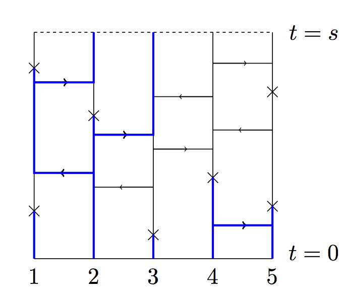
Figure 1. An instance of the graphical representation of the contact process on $V=\{1,\ldots,5\}$ with initial configuration $\textnormal{{1}}_{V}$. Note that $X_{s}=\textnormal{{1}}_{\{2,3\}}$.

Therefore, as described in Figure 1, we can read off the diagram starting from the bottom horizontal line and obtain $(X_{t})$. Construction of the graphical representation will play an important role in Sections A.2 and 6.3 when we introduce a decomposition of the contact process.

2.2. Random graphs and their limiting structure

Let $\mu$ be a probability distribution on $\mathbb{N}$. The random graph $G_{n}\sim\mathcal{G}(n,\mu)$ with degree distribution $\mu$ is defined as follows:

• Let $d_{i}\sim$ i.i.d.$\;\mu$ for $i=1,\ldots,n$, conditioned on $\sum_{i=1}^{n}d_{i}\equiv 0$ mod $2$. The numbers $d_{i}$ refer to the number of half-edges attached to vertex $i$.

• Generate the graph $G_{n}$ by pairing all half-edges uniformly at random.

The resulting graph $G_{n}$ is also called the configuration model. One may also be interested in the uniform model $G^{\textsf{u}}_{n}\sim\mathcal{G}^{\textsf{u}}(n,\mu)$, which picks a uniformly random simple graph among all simple graphs with degree sequence $\{d_{i}\}_{i\in[n]}\sim$ i.i.d.$\;\mu$. It is well-known that if $\mu$ has a finite second moment, then the two laws $\mathcal{G}(n,\mu)$ and $\mathcal{G}^{\textsf{u}}(n,\mu)$ are contiguous, in the sense that for any subset $A_{n}$ of graphs with $n$ vertices,

$$\mathbb{P}_{G_{n}\sim\mathcal{G}(n,\mu)}\left(G_{n}\in A_{n}\right)\rightarrow 0\quad\textnormal{implies}\quad\mathbb{P}_{G^{\textsf{u}}_{n}\sim\mathcal{G}^{\textsf{u}}(n,\mu)}\left(G^{\textsf{u}}_{n}\in A_{n}\right)\rightarrow 0.$$

For details, we refer the reader to Chapter 7 of [18] or to [7]. We remark that when $\mu=\textnormal{Pois}(d)$, the random graph $G_{n}\sim\mathcal{G}(n,\mu)$ is contiguous to the Erdős-Rényi random graph $G_{n}^{\textsc{er}}\sim\mathcal{G}_{\textsc{er}}(n,d/n)$ as shown in [8], Theorem 1.1.

Furthermore, it is also well-known that the random graph $G_{n}\sim\mathcal{G}(n,\mu)$ is locally tree-like, and the local neighborhoods converge locally weakly to Galton-Watson trees. To explain this precisely, let us denote the law of Galton-Watson tree with offspring distribution $\mu$ by $\textsf{\footnotesize{{GW}}}(\mu)$, and let $\textsf{\footnotesize{{GW}}}(\mu)^{l}$ be the law of $\textsf{\footnotesize{{GW}}}(\mu)$ truncated at depth $l$, that is, the vertices with distance $>l$ from the root are removed. Further, let $\widetilde{\mu}$ denote the size-biased distribution of $\mu$, defined by

(2.1) $$\widetilde{\mu}(k-1):=\frac{k\mu(k)}{\sum_{k^{\prime}=1}^{\infty}k^{\prime}\mu(k^{\prime})},\quad k=1,2,\ldots.$$

Note that if $\mu=$Pois$(d)$, then $\widetilde{\mu}=\mu$. Lastly, define $\textsf{\footnotesize{{GW}}}(\mu,\widetilde{\mu})^{l}$ to be the Galton-Watson process truncated at depth $l$, such that the root has offspring distribution $\mu$ while all other vertices have offspring distribution $\widetilde{\mu}$. Then the following lemma shows the convergence of local neighborhoods of $G_{n}$.

Lemma 2.1 ([3], Section 2.1).

Suppose that $\mu$ has a finite mean. Let $l>0$ and let $v$ denote the vertex in $G_{n}\sim\mathcal{G}(n,\mu)$ chosen uniformly at random. Then for any rooted tree $(T,x)$ of depth $l$, we have

$$\lim_{n\rightarrow\infty}\mathbb{P}((N(v,l),v)\cong(T,x))=\mathbb{P}_{(\mathcal{T},\rho)\sim\textsf{\footnotesize{{GW}}}(\mu,\widetilde{\mu})^{l}}((\mathcal{T},\rho)\cong(T,x)),$$

where $N(v,l)$ is the $l$-neighborhood of $v$ in $G_{n}$ and $\cong$ denotes the isomorphism of rooted graphs. We say that $G_{n}$ converges locally weakly to $\textsf{\footnotesize{{GW}}}(\mu,\widetilde{\mu})$.

We remark that the same holds for a fixed vertex $v\in G_{n}$. Moreover, we also stress that the condition for $\textsf{\footnotesize{{GW}}}(\mu,\widetilde{\mu})$ to be supercritical is equivalent to the condition for $\mathcal{G}(n,\mu)$ to have the unique giant component whp (see e.g., [14], or [4], Section 3 for details), which can be addressed as

(2.2) $$\mathbb{E}_{D\sim\mu}D(D-2)>0,$$

2.3. Notations

For a tree $T$ and a depth $l$, we denote by $T_{l}$ the set of vertices of $T$ at depth $l$. We use $T^{l}$ and $T_{\leq l}$ to denote the set of vertices of depth at most $l$. In particular, $\mathcal{T}^{l}\sim\textsf{\footnotesize{{GW}}}(\xi)^{l}$ denotes the Galton-Watson tree generated up to depth $l$, while the infinite Galton-Watson tree is denoted by $\mathcal{T}\sim\textsf{\footnotesize{{GW}}}(\xi)$.

Throughout the paper, we often work with the contact process defined on a (fixed) graph generated at random. To distinguish between the two randomness of different nature, we introduce the following notations:

• $\mathbb{P}_{\textsc{cp}}$ and $\mathbb{E}_{\textsc{cp}}$ denote the probability and the expectation, respectively, with respect to the randomness from contact processes

• $\mathbb{P}_{\textsc{gw}}$ and $\mathbb{P}_{\textsc{rg}}$ denote the probability with respect to the randomness from the underlying graph, when the graph is a Galton-Watson tree and a random graph $\mathcal{G}(n,\mu)$, respectively. We write $\mathbb{E}_{\textsc{gw}}$ and $\mathbb{E}_{\textsc{rg}}$ similarly for expectations.

• $\mathbb{P}$ and $\mathbb{E}$ denote the probability and expectation, respectively, with respect to the combined randomness over both the process and the graph. That is, for instance, $\mathbb{E}[\cdot]=\mathbb{E}_{\textsc{gw}}[\mathbb{E}_{\textsc{cp}}[\cdot]]$, if the underlying graph is a Galton-Watson tree.

3. Main concepts and ideas

Let us start by emphasizing that even though we borrow some ideas and notations from [2], this manuscript is self-contained and so the reader does not have to be familiar with [2] to read this manuscript. In this section, we briefly introduce the primary notions and discuss the main ideas in the paper. We also address the organization of the rest of the article in Section 3.4.

3.1. The root-added process and the lower bound of Theorem 1

In [2], Bhamidi and the authors studied the root-added contact process to prove $\lambda_{1}>0$ on $\textsf{\footnotesize{{GW}}}(\xi)$ with $\xi$ having an exponential tail. This notion continues to play a huge role in the current work as well, and hence we begin with explaining its definition and the concept of excursion time.

Definition 3.1 (Root-added contact process, [2]).

Let $T$ be a (finite or infinite) tree rooted at $\rho$. Let $T^{+}$ be the tree that has a parent vertex $\rho^{+}$ of $\rho$ which is connected only with $\rho$. The root-added contact process on $T$ is the continuous-time Markov chain on the state space $\{0,1\}^{T}$, defined as the contact process on $T^{+}$ with $\rho^{+}$ set to be infected permanently (hence we exclude $\rho^{+}$ from the state space). That is, $\rho^{+}$ is infected initially, and it does not have a recovery clock attached to itself. Let $\textsf{\small{{CP}}}^{\lambda}_{\rho^{+}}(T;x_{0})$ denote the root-added contact process on $T$ with initial condition $x_{0}\in\{0,1\}^{T}$. Note that the root-added contact process no longer has an absorbing state.

Definition 3.2 (Survival and excursion times).

Let $T$ be a (finite or infinite) tree rooted at $\rho$. The survival time and excursion time on $T$, denoted by $\textbf{R}(T)$ and $\textbf{S}(T)$, respectively, are defined as follows:

• $\textbf{R}(T)$ is the first time when the contact process $\textsf{\small{{CP}}}^{\lambda}(T;\textnormal{{1}}_{\rho})$ is all-healthy (i.e., when the process terminates). We also denote the expected survival time by $R(T)=\mathbb{E}_{\textsc{cp}}\textbf{R}(T)$.

• $\textbf{S}(T)$ is the first time when the root-added contact process $\textsf{\small{{CP}}}^{\lambda}_{\rho^{+}}(T;\textnormal{{1}}_{\rho})$ becomes all-healthy on $T$. We also denote the expected excursion time by $S(T)=\mathbb{E}_{\textsc{cp}}\textbf{S}(T)$.

Note that the quantities $R(T)$ and $S(T)$ are fixed numbers for each tree $(T,\rho)$ and satisfy $R(T)\leq S(T)$, which can be seen through the coupling via the graphical representation.

The previous work [2] established $\lambda_{1}>0$ by a recursive inequality on the depth of the tree that showed $\mathbb{E}\textbf{S}(\mathcal{T})<\infty$ for $\mathcal{T}\sim\textsf{\footnotesize{{GW}}}(\xi)$ with $\xi$ having an exponential tail decay. However, the argument had limitations since it could only deal with a small enough $\lambda$. In order to push its applicability to near-criticality, in Section 4 we introduce another recursive inequality based on fundamental properties of the contact process. Using the two different recursions, we can bound the tail probabilities of the expected excursion time, namely, $\mathbb{P}_{\textsc{gw}}(S(\mathcal{T})\geq t)$, and then the bound easily implies $\mathbb{E}_{\textsc{gw}}S(\mathcal{T})<\infty$. This is a substantial improvement from [2] where we could only control its expectation $\mathbb{E}_{\textsc{gw}}S(\mathcal{T})$ for small enough $\lambda$.

3.2. Deep infections, unicyclic neighbors and the lower bound of Theorem 2

To establish Theorem 2, we attempt to generalize Theorem 1 based on the fact that the local neighborhoods of $\mathcal{G}(n,\mu)$ look like Galton-Watson trees. There are two major obstacles on carrying out this idea.

1. For a vertex $v$ in $G\sim\mathcal{G}(n,\mu)$, its local neighborhood $N(v,l)$ contains a lot of cycles if $l\geq c_{\mu}\log n$ for some constant $c_{\mu}$.

2. Even for small $l$, there are $o(n)$ vertices that contain a cycle in $N(v,l)$.

3.2.1. Deep infections

To overcome the first issue, we show that the probability of having a deep infection of depth $\geq c_{\mu}\log n$ inside $\textsf{\small{{CP}}}^{\lambda}(\mathcal{T},\textnormal{{1}}_{\rho})$ is very small for a Galton-Watson tree $\mathcal{T}$. This leads to the consideration of the total infections at leaves of (finite) trees defined as follows.

Definition 3.3 (Total infections at leaves).

Let $T$ be a finite tree rooted at $\rho$, set $l:=\max\{\textnormal{dist}(\rho,v):v\in T\}$ be the depth of the tree and

$$\mathcal{L}:=\{v\in T:\textnormal{dist}(\rho,v)=l\}$$

be the collection of depth-$l$ leaves of $T$. Suppose that $l\geq 1$ and consider the root-added contact process $(X_{t})\sim\textsf{\small{{CP}}}^{\lambda}_{\rho^{+}}(T;\textnormal{{1}}_{\rho})$. For $v\in\mathcal{L}$, define the total infections at $v$, by

$$\textbf{M}^{l}_{v}(T):=\,\textnormal{the number of infections at }v\textnormal{ in }(X_{t})\textnormal{ during time }t\in[0,\textbf{S}(T)],$$

where $\textbf{S}(T)$ is the excursion time of $(X_{t})$. In other words, we count the number of times $t$ such that $X_{t}(v)=1$ and $X_{t-}(v)=0$ for $t\leq\textbf{S}(T)$. Then, we define the total infections at depth-$l$ leaves (during a single excursion) by

$$\textbf{M}^{l}(T)=\sum_{v\in\mathcal{L}}\textbf{M}^{l}_{v}(T).$$

For $l^{\prime}>l$, we set $\textbf{M}^{l^{\prime}}(T)\equiv 0$.

We also denote the expected total infections at depth-$l$ leaves by $M^{l}(T)=\mathbb{E}_{\textsc{cp}}\textbf{M}^{l}(T)$. Also, as above, we write $M^{l^{\prime}}(T)=0$ for $l^{\prime}>l$. Moreover, if the tree depth is $0$ (that is, $T$ is a single vertex), we set $\textbf{M}^{0}(T)\equiv 1$.

The previous work [2] derived an exponential decay of $\textbf{M}^{l}(\mathcal{T}^{l})$ in $l$ for $\mathcal{T}^{l}\sim\textsf{\footnotesize{{GW}}}(\widetilde{\mu})^{l}$ to deal with the same issue, but as before it had to require $\lambda$ to be small enough. However, unfortunately, the decay of $\textbf{M}^{l}(\mathcal{T}^{l})$ is insufficient for our purpose if $\lambda$ is close to $\lambda_{1}$, due to the reason we explain below.

If $\lambda=(1-\varepsilon)d^{-1}$ with $d=\mathbb{E}_{D\sim\widetilde{\mu}}D$, then for an infected vertex $v$ in $\mathcal{T}^{l}\sim\textsf{\footnotesize{{GW}}}(\widetilde{\mu})^{l}$, the expected number of offsprings of $v$ that get infected before $v$ becomes healthy is

$$\frac{\lambda d}{\lambda+1}\approx\frac{(1-\varepsilon)d}{d+1},\quad\textnormal{hence}\quad\mathbb{E}[\textbf{M}^{l}(\mathcal{T}^{l})]\geq\left(\frac{(1-\varepsilon)d}{d+1}\right)^{l},$$

and intuitively, the latter quantity essentially corresponds to $\mathbb{P}(\textbf{M}^{l}(\mathcal{T}^{l})\geq 1)$. To apply a union bound over all vertices in $G_{n}\sim\mathcal{G}(n,\mu)$, we need this probability to be of order $o(n^{-1})$. That is, we roughly require

$$l\gg\frac{\log n}{\log\{(1+\varepsilon)(1+d^{-1})\}}.$$

This is much larger than our budget $c_{\mu}\log n$ which is approximately $c\log_{d}n$. Thus, investigating the tail probability of $\textbf{M}^{l}(\mathcal{T}^{l})$ is not enough for our purpose. However, in [2], this approach was sufficient since we could set $\lambda$ as small as we wanted.

In Section 5, we instead focus on studying $\mathbb{P}_{\textsc{gw}}(M^{l}(\mathcal{T}^{l})\geq t)$, which turns out to have a much better bound than the tail of $\textbf{M}^{l}(\mathcal{T}^{l})$. Similarly as explained in Section 3.1, we derive two different recursive inequalities on $M^{l}(T)$ for a deterministic tree $T$, and prove its tail bound for the case of Galton-Watson trees.

3.2.2. Unicyclic neighbors

Another major issue is to deal with the neighborhoods $N(v,l)$ in $G_{n}\sim\mathcal{G}(n,\mu)$ containing a cycle. We rely on idea as [2], by observing that if $\mu$ satisfies (1.2), then there exists $\gamma(\mathfrak{c})>0$ such that whp, $N(v,\gamma\log_{d}n)$ contains at most one cycle for all $v$ with $d$ as in the previous subsection (see Lemma 6.11). Therefore, we study $S(T^{\prime})$ and $M^{l}(T^{\prime})$ as above (precise definitions are given in Section 6.1), for certain unicyclic graphs $T^{\prime}$ which are closely related to Galton-Watson trees. To this end, we appropriately cover $T^{\prime}$ by trees and deduce information on $S(T^{\prime})$ and $M^{l}(T^{\prime})$ from the results we obtained on trees. However, formalizing this idea requires a heavy technical work and it is presented in Appendix A. Similar ideas are applied to studying the contact process on $G_{n}$. Roughly speaking, we decompose $G_{n}$ by its local neighborhoods $\{N(v,l)\}_{v\in G_{n}}$, and derive results on $\textsf{\small{{CP}}}^{\lambda}(G_{n})$ by using what we know on $N(v,l)$.

3.3. The proof of Theorems 5 and 6

The previous work [2] settled that $\lambda_{c}^{+}(\mu)<\infty$, which was based on a challenging structural analysis on the configuration model. Roughly speaking, they showed the existence of an embedded expander, a subset of large degree vertices in the random graph, on which it is easy to send infections from one vertex to another. Upon establishing its existence, spreading infections on the embedded expander could then be done by a relatively straight-forward way, which was to infect a site at distance $l$ with probability $(c(1-e^{-\lambda}))^{l}$, since we could choose $\lambda$ to be large. One of the main difficulties in establishing the much improved bound $\lambda_{c}^{+}(\mu)\leq\lambda_{1}^{\textsc{gw}}(\widetilde{\mu})$ is that we need to develop a more efficient way of sending infections from a vertex to another.

The key observation for such improvement is that if $\lambda>\lambda_{1}^{\textsc{gw}}(\widetilde{\mu})$, the expected number of infections on $\mathcal{T}\sim\textsf{\footnotesize{{GW}}}(\widetilde{\mu})$ grows exponentially in time (Lemmas 7.5 and 7.6). We use this property as our driving force of passing infections on the random graph, which is possible since the local neighborhoods look like Galton-Watson trees. This new method turns out to be substantially better than the aforementioned approach.

However, since we now need to reveal the neighborhoods to check if the infections spread well, the structural analysis on the random graph becomes even more involved than the previous proof in [2]. We carry out by introducing an appropriate notion of good vertices, which roughly refer to the sites that are capable of propagating enough infections around them, and showing that any set of $\delta n$ infected good vertices causes $\geq 2\delta n$ good vertices to be infected at a later time with high probability except for an exponentially small error.

3.4. Organization of the article

Sections 4–6 are devoted to the derivation of the lower bounds of Theorems 1 and 2. In Section 4, we introduce the basic form of the recursion argument on Galton-Watson trees and establish the lower bound of Theorem 1. In Section 5, we extend the recursion criterion to the study of deep infections. Section 6 then concludes the proof of the lower bound of Theorem 2, while the technical works needed to study the unicyclic graphs are deferred to Appendix A. Finally, we finish the proof of Theorems 1 and 2 by settling their upper bounds in Section 7.

4. Survival and excursion times on trees

In this section, we introduce primary recursive argument on the expected excursion time which are used throughout the paper. In Section 4.1, we review some ideas developed in [2], and derive another recursive inequality on excursion times. In Sections 4.2 and 4.3, we prove a tail probability estimate and establish Theorem 1 as its application.

4.1. Deterministic recursions on trees

Let $T$ be a finite tree rooted at $\rho$ and recall the definition of the root-added contact process $\textsf{\small{{CP}}}^{\lambda}_{\rho^{+}}(T^{+};x_{0})$ (Definition 3.1). Let $R(T)$ and $S(T)$ be expected survival and recursion time as in Definition 3.2.

In $(T,\rho)$, let $D=\text{deg}(\rho)$ and $v_{1},\ldots,v_{D}$ be the children of $\rho$. Further, let $T_{1},\ldots,T_{D}$ be the subtrees from each child of $\rho$, rooted at $v_{1},\ldots,v_{D}$, respectively. In [2], we proved the following recursion on the excursion times.

Proposition 4.1 ([2], Lemma 3.3).

Let $T$ and $T_{1},\ldots,T_{D}$ be as above. Then, the expected excursion times $S(T)$ and $S(T_{1}),\ldots,S(T_{D})$ satisfy

(4.1) $$S(T)\leq\prod_{i=1}^{D}(1+\lambda S(T_{i})).$$

Even though the proof can be found in [2], we briefly explain it again, mainly because the ideas will be revisited in Proposition 5.2. For a detailed proof, we refer to [2].

Proof.

Consider $\textsf{\small{{CP}}}^{\lambda}_{\rho}(T_{i};\textnormal{{1}}_{v_{i}})$ (the subscript $\rho$ indicates that it serves as the added parent above $v_{i}$), the root-added contact process on each $T_{i}$, and their product

(4.2) $$\textsf{\small{{CP}}}^{\otimes}(T;\textnormal{{1}}_{v_{i}}):=\left(\otimes_{\begin{subarray}{c}j=1\\ j\neq i\end{subarray}}^{D}\textsf{\small{{CP}}}^{\lambda}_{\rho}(T_{j};\textnormal{{0}})\right)\otimes\textsf{\small{{CP}}}^{\lambda}_{\rho}(T_{i};\textnormal{{1}}_{v_{i}}),$$

for each $i\in[D]$. Let $\textbf{S}_{i}^{\otimes}$ denote the excursion time of this process, that is, the first return time to the all-healthy state $\otimes_{j=1}^{D}\textnormal{{0}}_{T_{j}}$, and let $S_{i}^{\otimes}=\mathbb{E}_{\textsc{cp}}\textbf{S}_{i}^{\otimes}$. Further, define the average of $S_{i}^{\otimes}$ by

(4.3) $$S^{\otimes}=\frac{1}{D}\sum_{i=1}^{D}S_{i}^{\otimes}.$$

Then, we can control $S(T)$ by $S^{\otimes}$, based on the following modification of the process $\textsf{\small{{CP}}}^{\lambda}_{\rho^{+}}(T;\textnormal{{1}}_{\rho})$ introduced in [2], Lemma 3.3.

• Consider the process $(X^{\sharp}_{t})$ on $T$ that follows the same transition rule as $\textsf{\small{{CP}}}^{\lambda}_{\rho^{+}}(T;\textnormal{{1}}_{\rho})$, except for the recoveries at root $\rho$.

• An independent rate-$1$ Poisson clock is associated with $\rho$, and the recovery at $\rho$ is only valid if $X^{\sharp}_{t}=\textnormal{{1}}_{\rho}$ when the clock rings at time $t$.

In other words, $(X^{\sharp}_{t})$ is generated by ignoring the recoveries of $(X_{t})\sim\textsf{\small{{CP}}}^{\lambda}_{\rho^{+}}(T;\textnormal{{1}}_{\rho})$ at $\rho$ if there is another infected vertex at the time of recovery. Let us denote the expected excursion time of this process by $S^{\sharp}(T)$. Recalling the coupling argument using the graphical representation (Section 2.1), we know that $S^{\sharp}(T)\geq S(T)$. Moreover, an excursion of $(X^{\sharp}_{t})$ can be described as follows.

1. Initially $X^{\sharp}_{0}=\textnormal{{1}}_{\rho}$, and we terminate if $\rho$ gets healed before infecting any of its children. Otherwise, suppose that the first child to receive an infection from $\rho$ is $v_{i}$.

2. Since $\rho$ stays infected until everyone else is healthy, it is the same as running an excursion of $\textsf{\small{{CP}}}^{\otimes}(T;\textnormal{{1}}_{v_{i}})$. When the excursion is finished, we go back to Step 1.

The probability that we terminate at Step 1 is $(1+\lambda D)^{-1}$. So an excursion of $(X^{\sharp}_{t})$ is a series of excursions of $\{\textsf{\small{{CP}}}^{\otimes}(T;\textnormal{{1}}_{v_{i}})\}_{i}$, until we stop when having a successful coin toss of probability $(1+\lambda D)^{-1}$ after each of the excursion. Furthermore, note that the expected waiting time to see either a recovery at $\rho$ or an infection at a child is $(1+\lambda D)^{-1}$. Therefore, we obtain that

(4.4) $$S(T)\leq S^{\sharp}(T)=\sum_{k=0}^{\infty}\left(\frac{1}{1+\lambda D}\right)\left(\frac{\lambda D}{1+\lambda D}\right)^{k}\left[\frac{k+1}{1+\lambda D}+kS^{\otimes}\right]=1+\lambda DS^{\otimes}.$$

The final step is to consider the stationary distributions of $\textsf{\small{{CP}}}^{\lambda}_{\rho}(T_{i})$ and their product. Let $\pi_{i}$ be the stationary distribution of $\textsf{\small{{CP}}}^{\lambda}(T_{i})$. Then, $\pi_{i}(\textnormal{{0}})$ corresponds to the fraction of time that $\textsf{\small{{CP}}}^{\lambda}(T_{i})$ is at state 0, and hence

(4.5) $$\pi_{i}(\textnormal{{0}})=\frac{\lambda^{-1}}{S(T_{i})+\lambda^{-1}}=\frac{1}{1+\lambda S(T_{i})}.$$

Similarly, the stationary distribution $\pi^{\otimes}$ of $\textsf{\small{{CP}}}^{\otimes}(T)$ satisfies

(4.6) $$\pi^{\otimes}(\textnormal{{0}})=\frac{(\lambda D)^{-1}}{(\lambda D)^{-1}+S^{\otimes}}=\frac{1}{1+\lambda DS^{\otimes}}.$$

Since $\pi^{\otimes}=\otimes_{i=1}^{D}\pi_{i}$, this implies

(4.7) $$1+\lambda DS^{\otimes}=\prod_{i=1}^{D}(1+\lambda S(T_{i})).$$

Therefore, we plug this into (4.4) and obtain the conclusion. ∎

Unfortunately, having (4.1) is insufficient for our purpose. One can see this by taking expectation on each side of (4.1) over $T\sim\textsf{\footnotesize{{GW}}}(\xi)$. In order to yield a meaningful recursion, $\lambda$ should be small in terms of the exponential moment of $\xi$, which has nothing to do with $1/\mathbb{E}\xi$ in general (for details, see the proof of [2], Lemma 3.3). Therefore, we develop another recursion which redeems (4.1). Our first step is to build up a recursion regarding $R(T)$, the expected survival time.

Proposition 4.2.

Let $T_{1},\ldots,T_{D}$ be as Proposition 4.1, and assume that $\lambda^{2}\sum_{i=1}^{D}R(T_{i})<1$. Then,

(4.8) $$R(T)\leq\frac{1+\lambda\sum_{i=1}^{D}R(T_{i})}{1-\lambda^{2}\sum_{i=1}^{D}R(T_{i})}.$$

Proof.

Suppose that we run $\textsf{\small{{CP}}}^{\lambda}(T;\textnormal{{1}}_{\rho})$. In the beginning, which we call the first round, the infection at the root stays there for a while, then it may infect some the children. If a children $v_{i}$ gets infected, then we can think of it as running a new contact process $\textsf{\small{{CP}}}^{\lambda}(T_{i};\textnormal{{1}}_{v_{i}})$. Here, we should also consider the effect of $v_{i}$ infecting $\rho$ again, and if this happens, the reinfected $\rho$ starts the second round of the dynamics.

The expected survival time of the first round is bounded by

$$1+\lambda\sum_{i=1}^{D}R(T_{i}),$$

since the expected survival time of the root is $1$ and it sends infections $\lambda$ times in expectation to each children before dying out. Similarly, the expected number of infections sent from the children $\{v_{i}\}$ to $\rho$ in the first round is bounded by

$$\lambda^{2}\sum_{i=1}^{D}R(T_{i}).$$

Therefore, we obtain that

$$R(T)\leq 1+\lambda\sum_{i=1}^{D}R(T_{i})+\left\{\lambda^{2}\sum_{i=1}^{D}R(T_{i})\right\}R(T),$$

and the conclusion follows since we assumed $\lambda^{2}\sum_{i=1}^{D}R(T_{i})<1$. ∎

We are now interested in the relation between $R(T)$ and $S(T)$.

Proposition 4.3.

On a finite rooted tree $(T,\rho)$, let $R(T)$ and $S(T)$ be the expected survival time of $\textsf{\small{{CP}}}^{\lambda}(T;\textnormal{{1}}_{\rho})$ and the expected excursion time of $\textsf{\small{{CP}}}^{\lambda}_{\rho^{+}}(T;\textnormal{{1}}_{\rho})$, respectively. Then, we have

(4.9) $$\frac{S(T)}{1+\lambda S(T)}\leq R(T).$$

Proof.

Suppose that we are running a root-added contact process $(X_{t})\sim\textsf{\small{{CP}}}^{\lambda}_{\rho^{+}}(T;\textnormal{{1}}_{\rho})$ until time $t_{0}$. Further, let

$$A_{t_{0}}=\{t\leq t_{0}:X_{t}\neq\textnormal{{0}}\},$$

and let $|A_{t_{0}}|$ be the Lebesgue measure of the set $A_{t_{0}}$. In the root-added contact process, after one excursion we wait $(1/\lambda)$-time in expectation until we start the next excursion. Therefore, we have

(4.10) $$\lim_{t_{0}\rightarrow\infty}\frac{\mathbb{E}_{\textsc{cp}}|A_{t_{0}}|}{t_{0}}=\frac{S(T)}{\lambda^{-1}+S(T)}=\frac{\lambda S(T)}{1+\lambda S(T)}.$$

On the other hand, $\textsf{\small{{CP}}}^{\lambda}_{\rho^{+}}(T;\textnormal{{1}}_{\rho})$ can be considered as the contact process $\textsf{\small{{CP}}}^{\lambda}(T;\textnormal{{1}}_{\rho})$ of which the root $\rho$ receives new infections at every ring of an independent Poisson process with rate $\lambda$. Since the rate-$\lambda$ Poisson process rings $\lambda t_{0}$ times in expectation until time $t_{0}$, we see that

$$\mathbb{E}_{\textsc{cp}}|A_{t_{0}}|\leq\lambda t_{0}R(T).$$

Comparing this to (4.10), we obtain that

$$\frac{\lambda S(T)}{1+\lambda S(T)}\leq\lambda R(T),$$

implying the conclusion. ∎

Combining Propositions 4.2 and 4.3, we obtain that

(4.11) $$\begin{split}S(T)\leq\frac{R(T)}{1-\lambda R(T)}&\leq\frac{1+\lambda\sum_{i=1}^{D}R(T_{i})}{1-\lambda-2\lambda^{2}\sum_{i=1}^{D}R(T_{i})}\\ &\leq\frac{1+\lambda\sum_{i=1}^{D}S(T_{i})}{1-\lambda-2\lambda^{2}\sum_{i=1}^{D}S(T_{i})},\end{split}$$

provided that $\lambda+2\lambda^{2}\sum_{i=1}^{D}S(T_{i})<1$. In the rest of the paper, (4.1) and (4.11) serve as two major recursive inequalities for $S(T)$.

4.2. Recursive tail estimate for Galton-Watson trees

In this subsection, we establish the primary tail probability estimate on $S(\mathcal{T})$ for a Galton-Watson tree $\mathcal{T}$, and prove Theorem 1 as its application.

Let $\xi$ be an integer-valued random variable that satisfy the concentration condition (1.2) for $\mathfrak{c}=\{c_{\delta}\}_{\delta\in(0,1]}$. For the Galton-Watson tree $\mathcal{T}\sim\textsf{\footnotesize{{GW}}}(\xi)$, the expected excursion time $S(\mathcal{T})$ is now a random variable driven by the randomness from $\textsf{\footnotesize{{GW}}}(\xi)$. The goal of this subsection is to show that $S(\mathcal{T})$ is finite almost surely if $\lambda\leq(1-\varepsilon)d^{-1}$, where $\varepsilon>0$ is an arbitrarily fixed constant and $d=\mathbb{E}\xi$ is large enough depending on $\varepsilon$. We establish this by proving that the upper tail of $S(\mathcal{T})$ is very light. In what follows, we denote the law of Galton-Watson trees of depth $l$ by $\textsf{\footnotesize{{GW}}}(\xi)^{l}$.

Theorem 4.4.

Let $l\geq 0$ be an integer, $\varepsilon\in(0,1)$ and $\mathfrak{c}=\{c_{\delta}\}_{\delta\in(0,1]}$ be a collection of positive constants. Then there exists $d_{0}(\varepsilon,\mathfrak{c})>0$ such that the following holds true. For any $\xi$ that satisfies $d:=\mathbb{E}\xi\geq d_{0}$ and (1.2) with $\mathfrak{c}$, we have for $\lambda=(1-\varepsilon)d^{-1}$ and $\mathcal{T}^{l}\sim\textsf{\footnotesize{{GW}}}(\xi)^{l}$ that

(4.12) $$\mathbb{P}_{\textsc{gw}}\left(S(\mathcal{T}^{l})\geq t\right)\leq t^{-\sqrt{d}}(\log t)^{-2}\leavevmode\nobreak\ \leavevmode\nobreak\ \leavevmode\nobreak\ \textnormal{for all }t\geq\frac{2}{\varepsilon},$$

where $S(\mathcal{T}^{l})$ is the expected excursion time on $\mathcal{T}^{l}$.

Remark 4.5.

The term $(\log t)^{-2}$ in the r.h.s. of (4.12) may look useless, but this plays a key role in carrying out an inductive argument (see Lemma 4.8). We remark that the exponent $-2$ of $(\log t)^{-2}$ can be replaced by any number smaller than $-1$. Moreover, the exponent $\sqrt{d}$ can be replaced by any term of order $O(d^{1-\eta})$ for $\eta>0$.

The rest of the subsection is devoted to the proof of Theorem 4.4. We do this by an induction on $l$, the tree depth. If $l=0$, $\mathcal{T}^{0}$ is just a single vertex $\rho$ and hence $S(\mathcal{T}^{0})\equiv 1$, implying (4.12).

Suppose that we have (4.12) for $l$. Let $(\mathcal{T}^{l+1},\rho)\sim\textsf{\footnotesize{{GW}}}(\xi)^{l+1}$, and set $D=\text{deg}(\rho)\overset{\textnormal{d}}{=}\xi$. As before, let $T_{i},\;i\in[D]$ denote the subtrees of $\mathcal{T}^{l+1}$, rooted at the child $v_{i}$. Let $c_{1}$ be the constant in $\mathfrak{c}$ with $\delta=1$, and we divide $t$ into three regimes as follows.

• (small) $2/\varepsilon\leq t\leq d^{\frac{1}{10}}$;

• (intermediate) $d^{\frac{1}{10}}\leq t\leq\exp(\frac{1}{2}c_{1}\sqrt{d})$;

• (large) $\exp(\frac{1}{2}c_{1}\sqrt{d})\leq t$.

Then, we establish (4.12) on each regime separately. As the proof goes on, we will figure out the conditions for $d_{0}(\varepsilon,\mathfrak{c})$ as well.

Remark 4.6.

There is much freedom in choosing $d^{\frac{1}{10}}$, the threshold between the small and intermediate regime. Indeed, any $d^{\eta}$ with $\eta\in(0,\;1-d^{-1/2})$ would work for our purpose. However, the specific choice of $d^{1/10}$ will turn out to be useful later, in the proof of Proposition 6.4 and Lemma A.5. The choice of $\exp(\frac{1}{2}c_{1}\sqrt{d})$ will be clear in (4.22).

4.2.1. Proof of Theorem 4.4 for small $t$

To show (4.12) for small $t$, we rely on (4.11). For $\mathcal{T}^{l+1}\sim\textsf{\footnotesize{{GW}}}(\xi)^{l+1}$ and $T_{i},\;i\in[D]$ as above, suppose that

$$\sum_{i=1}^{D}S(T_{i})\leq\frac{2d}{\varepsilon}\left(1+\frac{\varepsilon}{3}\right).$$

Then, from (4.11) and a little bit of algebra we see that

$$S(\mathcal{T}^{l+1})\leq\frac{1+\lambda\frac{2d}{\varepsilon}\left(1+\frac{\varepsilon}{3}\right)}{1-\lambda-2\lambda^{2}\frac{2d}{\varepsilon}\left(1+\frac{\varepsilon}{3}\right)}\leq\frac{\frac{2}{\varepsilon}-\frac{1}{3}}{1-\frac{7}{d\varepsilon}}<\frac{2}{\varepsilon},$$

where the last inequality holds if

(4.13) $$d\geq\frac{42}{\varepsilon^{2}}.$$

Therefore, for $d$ with (4.13), we have

(4.14) $$\mathbb{P}_{\textsc{gw}}\left(S(\mathcal{T}^{l+1})\geq\frac{2}{\varepsilon}\right)\leq\mathbb{P}\left(D\geq\left(1+\frac{\varepsilon}{6}\right)d\right)+\mathbb{P}_{\textsc{gw}}\left(\sum_{i=1}^{(1+\frac{\varepsilon}{6})d}S(T_{i})\geq\frac{2d}{\varepsilon}\left(1+\frac{\varepsilon}{3}\right)\right),$$

where $T_{i},\;i\in\mathbb{N}$ are i.i.d. $\textsf{\footnotesize{{GW}}}(\xi)^{l}$. By the assumption on $\xi$, we can bound the first term in the r.h.s. by

(4.15) $$\mathbb{P}\left(D\geq\left(1+\frac{\varepsilon}{6}\right)d\right)\leq\exp\left(-c_{\varepsilon^{\prime}}d\right),$$

for $\varepsilon^{\prime}=\varepsilon/6$. To deal with the second term, the induction hypothesis tells us that the c.d.f. of $S(T_{i})$ has an upper bound

$$\mathbb{P}_{\textsc{gw}}(S(T_{i})\geq s)\leq s^{-\sqrt{d}}$$

for all $s\geq 2/\varepsilon$, and hence we can apply the following lemma.

Lemma 4.7.

Let $\varepsilon\in(0,1)$ be a given constant. Then there exists $d_{1}>0$ independent of $\varepsilon$ such that the following holds for all $d\geq d_{1}$. Let $Z_{i},\;i\in\mathbb{N}$ be i.i.d. positive random variables that satisfies

(4.16) $$\mathbb{P}\left(Z_{i}\geq t\right)\leq 5t^{-\sqrt{d}},\quad\textnormal{for all }t\geq\frac{2}{\varepsilon}.$$

Then, we have

(4.17) $$\begin{split}\mathbb{P}\left(\sum_{i=1}^{(1+\frac{\varepsilon}{6})d}Z_{i}\geq\frac{2d}{\varepsilon}\left(1+\frac{\varepsilon}{3}\right)\right)\leq\frac{1}{2}d^{-\frac{1}{10}\sqrt{d}}\left(\frac{1}{10}\log d\right)^{-2}.\end{split}$$

We defer the proof of this lemma until Section 4.3, since it is essentially a special case of Lemma 4.8 below.

Thanks to Lemma 4.7, we combine (4.14), (4.15) and (4.17) to obtain that

(4.18) $$\mathbb{P}_{\textsc{gw}}\left(S(\mathcal{T}^{l+1})\geq\frac{2}{\varepsilon}\right)\leq\exp(-c_{\varepsilon^{\prime}}d)+\frac{1}{2}d^{-\frac{1}{10}\sqrt{d}}\left(\log d^{\frac{1}{10}}\right)^{-2}\leq d^{-\frac{1}{10}\sqrt{d}}\left({\frac{1}{10}}\log d\right)^{-2},$$

for $d$ satisfying

(4.19) $$\exp(-c_{\varepsilon^{\prime}}d)\leq\frac{1}{2}d^{-\frac{1}{10}\sqrt{d}}\left({\frac{1}{10}}\log d\right)^{-2}.$$

Finally, we clearly see that (4.18) settles (4.12) for all small $t$, namely, $2/\varepsilon\leq t\leq d^{\frac{1}{10}}$.

4.2.2. Proof of Theorem 4.4 for intermediate $t$

For $t\geq d^{\frac{1}{10}}$, we use (4.1). That is, we attempt to control

(4.20) $$\mathbb{P}_{\textsc{gw}}\left(S(\mathcal{T}^{l+1})\geq t\right)\leq\mathbb{P}_{\textsc{gw}}\left(\sum_{i=1}^{D}\log(1+\lambda S(T_{i}))\geq\log t\right).$$

Let $c_{1}$ be the constant given from the assumption of Theorem 4.4 (with $\delta=1$). Note that we can split the event in the r.h.s. as follows.

(4.21) $$\mathbb{P}_{\textsc{gw}}\left(S(\mathcal{T}^{l+1})\geq t\right)\leq\mathbb{P}\left(D\geq 2d\right)+\mathbb{P}_{\textsc{gw}}\left(\sum_{i=1}^{2d}\log(1+\lambda S(T_{i}))\geq\log t\right).$$

The concentration assumption (1.2) on $\xi$ tells us that the first term is bounded by

(4.22) $$\mathbb{P}(D\geq 2d)\leq\exp(-c_{1}d)\leq\frac{1}{2}t^{-\sqrt{d}}(\log t)^{-2},\quad\textnormal{for }t\leq e^{\frac{1}{2}c_{1}\sqrt{d}}.$$

To control the second term in the r.h.s. of (4.21), we use the following lemma.

Lemma 4.8.

Let $\varepsilon\in(0,1)$ be a given constant. Then there exists $d_{1}(\varepsilon)>0$ such that the following holds true for all $d\geq d_{1}$. Let $Z_{i},\;i\in\mathbb{N}$ be i.i.d. positive random variables that satisfies

(4.23) $$\mathbb{P}(Z_{i}\geq t)\leq 5t^{-\sqrt{d}}(\log t)^{-2},\leavevmode\nobreak\ \leavevmode\nobreak\ \leavevmode\nobreak\ \textnormal{for all }t\geq\frac{3}{\varepsilon}.$$

Then, for all $t\geq d^{\frac{1}{10}}$, we have

(4.24) $$\mathbb{P}\left(\sum_{i=1}^{2d}\log\left(1+\frac{4}{d}Z_{i}\right)\geq\log\left(\frac{t}{2}\right)\right)\leq\frac{1}{2}t^{-\sqrt{d}}(\log t)^{-2}.$$

The proof of Lemma 4.8 is postponed until Section 4.3, since it requires a substantial technical work. Note that (4.24) contains a slightly more generalized form than the r.h.s. of (4.21), which will be useful in Sections 5 and 6.

To conclude the proof for intermediate $t$, (4.21), (4.22) and (4.24) together deduce (4.12) for $t\geq d^{\frac{1}{10}}$. Here, the constant $d_{0}$ in the statement of the theorem should satisfy $d_{0}\geq d_{1}$ for $d_{1}$ in Lemma 4.8.

4.2.3. Proof of Theorem 4.4 for large $t$

For $t\geq\exp(\frac{1}{2}c_{1}\sqrt{d})$, we again attempt to control (4.20). Let

$$\Delta_{d,t}=\frac{4\sqrt{d}}{c_{1}}\log t,$$

and note that we can split the event in the r.h.s. of (4.20) as follows.

(4.25) $$\begin{split}\mathbb{P}_{\textsc{gw}}\left(S(\mathcal{T}^{l+1})\geq t\right)\leq&\;\mathbb{P}\left(D\geq\Delta_{d,t}\right)+\mathbb{P}_{\textsc{gw}}\left(\sum_{i=1}^{2d}\log(1+\lambda S(T_{i}))\geq\log t\right)\\ &+\sum_{2d\,\leq\,r\,\leq\,\Delta_{d,t}}\mathbb{P}(D\geq r)\times\mathbb{P}_{\textsc{gw}}\left(\sum_{i=1}^{r}\log(1+\lambda S(T_{i}))\geq\log t\right).\end{split}$$

The concentration assumption (1.2) on $\xi$ tells us that for $t\geq\exp(\frac{1}{2}c_{1}\sqrt{d})$,

(4.26) $$\begin{split}\mathbb{P}\left(D\geq\Delta_{d,t}\right)\leq\mathbb{P}\left(D\geq d+\frac{\Delta_{d,t}}{2}\right)\leq\exp\left(-2\sqrt{d}\log t\right)\leq\frac{1}{4}t^{-\sqrt{d}}(\log t)^{-2},\end{split}$$

where the last inequality is satisfied by large $d$. This controls the first term in the r.h.s. of (4.25). The second term is then estimated by Lemma 4.8, which gives

(4.27) $$\mathbb{P}_{\textsc{gw}}\left(\sum_{i=1}^{2d}\log(1+\lambda S(T_{i}))\geq\log t\right)\leq\frac{1}{2}t^{-\sqrt{d}}(\log t)^{-2}.$$

To bound the last term, we use the following lemma.

Corollary 4.9.

Let $\varepsilon\in(0,1)$ be a given constant. Then there exist $d_{1}(\varepsilon)>0$ and an absolute constant $C_{1}>0$ such that the following holds true for all $d\geq d_{1}$. Let $Z_{i},\;i\in\mathbb{N}$ be i.i.d. positive random variables that satisfies

$$\mathbb{P}(Z_{i}\geq t)\leq 5t^{-\sqrt{d}}(\log t)^{-2},\leavevmode\nobreak\ \leavevmode\nobreak\ \leavevmode\nobreak\ \textnormal{for all }t\geq\frac{3}{\varepsilon}.$$

Then, for all $t\geq\exp(\frac{1}{2}c_{1}\sqrt{d})$ and $2d\leq r\leq\Delta_{d,t}$ with $\Delta_{d,t}$ as above, we have

(4.28) $$\mathbb{P}\left(\sum_{i=1}^{r}\log\left(1+\frac{4}{d}Z_{i}\right)\geq\log\left(\frac{t}{2}\right)\right)\leq t^{-\sqrt{d}}(\log t)^{-2}\exp\left(\frac{C_{1}r}{\varepsilon\sqrt{d}}\right).$$

The proof of Corollary 4.9 is postponed until Section 4.3, which will be proven together with Lemma 4.8.

To conclude the proof of Theorem 4.4 for large $t$, observe that for $2d\leq r\leq\Delta_{d,t}$

$$\mathbb{P}(D\geq r)\leq\mathbb{P}\left(D\geq d+\frac{r}{2}\right)\leq\exp\left(-\frac{c_{1}r}{2}\right),$$

by the concentration condition (1.2) of $D$. Therefore, for sufficiently large $d$, we have by (4.28) that

$$\mathbb{P}(D\geq r)\times\mathbb{P}_{\textsc{gw}}\left(\sum_{i=1}^{r}\log(1+\lambda S(T_{i}))\geq\log t\right)\leq t^{-\sqrt{d}}(\log t)^{-2}\exp\left(-\frac{c_{1}r}{4}\right).$$

Along with (4.25), (4.26) and (4.27), this proves Theorem 4.4 for $t\geq\exp(\frac{1}{2}c_{1}\sqrt{d})$. ∎

As the first application of Theorem 4.4, we establish Theorem 1.

Proof of Theorem 1: the lower bound.

Let $\varepsilon\in(0,1)$ be an arbitrary constant and suppose that the collection of distributions $\{\xi_{k}\}_{k}$ satisfies (1.2) for $\mathfrak{c}=\{c_{\delta}\}_{\delta\in(0,1]}$. Let $d_{0}=d_{0}(\varepsilon,\mathfrak{c})$ as in Theorem 4.4, and assume that $\mathbb{E}\xi_{k}\geq d_{0}$. Then, Theorem 4.4 implies that for $\textsf{\small{{CP}}}^{\lambda}_{\rho^{+}}(\mathcal{T}^{l}_{k};\textnormal{{1}}_{\rho})$ on $\mathcal{T}_{k}\sim\textsf{\footnotesize{{GW}}}(\xi_{k})^{l}$ with intensity $\lambda=(1-\varepsilon)(\mathbb{E}\xi_{k})^{-1}$, we have

$$\mathbb{E}_{\textsc{gw}}\left[S(\mathcal{T}^{l}_{k})\right]<\frac{3}{\varepsilon}.$$

Thus, we deduce that the expected survival time of $\textsf{\small{{CP}}}^{\lambda}(\mathcal{T}^{l}_{k};\textnormal{{1}}_{\rho})$ is also

$$\mathbb{E}_{\textsc{gw}}\left[R(\mathcal{T}^{l}_{k})\right]<\frac{3}{\varepsilon}.$$

Therefore, by the monotone convergence theorem, we have that for $\mathcal{T}_{k}\sim\textsf{\footnotesize{{GW}}}(\xi_{k})$,

$$\mathbb{E}_{\textsc{gw}}[R(\mathcal{T}_{k})]=\lim_{l\rightarrow\infty}\mathbb{E}_{\textsc{gw}}[R(\mathcal{T}_{k}^{l})]\leq\frac{3}{\varepsilon},$$

and hence the survival time $\textbf{R}(\mathcal{T}_{k})$ is finite almost surely, which implies that

$$\lambda=\frac{1-\varepsilon}{\mathbb{E}\xi_{k}}\leq\lambda_{1}^{\textsc{gw}}(\xi_{k}),$$

for all large enough $k$. ∎

4.3. Proof of the induction lemmas

To conclude Section 4, we discuss the proof of Lemmas 4.7, 4.8 and Corollary 4.9. We first establish Lemma 4.8 and Corollary 4.9 together, and then the proof of Lemma 4.7 will follow based on similar ideas.

Proof of Lemma 4.8 and Corollary 4.9.

We first set

(4.29) $$Y_{i}=\log\left(1+\frac{4Z_{i}}{d}\right),\quad\Delta_{d,t}=\frac{4\sqrt{d}}{c_{1}}\log t,\quad\textnormal{and let}\quad 2d\leq r\leq 2d\,\vee\Delta_{d,t}.$$

We will attempt to find an upper bound of

(4.30) $$\mathbb{P}\left(\sum_{i=1}^{r}\log\left(1+\frac{4}{d}Z_{i}\right)\geq\log\left(\frac{t}{2}\right)\right),$$

to cover the case of Corollary 4.9 as well.

Note that the assumption (4.23) on $Z_{i}$ gives us $\mathbb{E}Z_{i}\leq\frac{4}{\varepsilon}$. Based on (4.23), we can find an upper bound for $\mathbb{E}Y_{i}$ by

(4.31) $$\mathbb{E}Y_{i}\leq\log\mathbb{E}e^{Y_{i}}=\log\left(1+\frac{4\mathbb{E}Z_{i}}{d}\right)\leq\log\left(1+\frac{16}{\varepsilon d}\right)\leq\frac{16}{\varepsilon d}.$$

Further, (4.23) tells us that the tail of $Y_{i}$ is bounded by

(4.32) $$\mathbb{P}(Y_{i}\geq s)=\mathbb{P}\left(Z_{i}\geq\frac{d}{4}(e^{s}-1)\right)\leq 5\left(\frac{d}{4}(e^{s}-1)\right)^{-\sqrt{d}}\left\{\log\left(\frac{d}{4}(e^{s}-1)\right)\right\}^{-2}.$$

In order to have $\sum_{i=1}^{r}Y_{i}\geq\log(t/2)$ for $t\geq\sqrt{d}$ and $r\leq 2d\vee\Delta_{d,t}$, we need to have some of $Y_{i}$ being larger than $\frac{\log d}{80d}$. In the following, $k$ denotes the number of $Y_{i}$ that are at least $\frac{\log d}{80d}$. Note that in this case, the sum over all $Y_{i}$ that are smaller than $\frac{\log d}{80d}$ is at most

(4.33) $$(2d\vee\Delta_{d,t})\cdot\frac{\log d}{80d}=\frac{1}{40}\log d\,\vee\frac{\log d}{20c_{1}\sqrt{d}}\log t=:m(d,t).$$

Then, we can split the probability in (4.30) as follows.

(4.34) $$\begin{split}&\mathbb{P}\left(\sum_{i=1}^{r}Y_{i}\geq\log\left(\frac{t}{2}\right)\right)\\ &\leq\sum_{k=1}^{r}{r\choose k}\sum_{j=1}^{m(d,t)+1}\mathbb{P}\left(\sum_{i=1}^{k}Y_{i}\geq\log\left(\frac{t}{2}\right)-j\;;\;Y_{i}\geq\frac{\log d}{80d},\;\forall i\leq k\right)\;\\ &\qquad\qquad\qquad\qquad\qquad\times\mathbb{P}\left(\sum_{i=k+1}^{r}Y_{i}\geq j-1\;;\;Y_{i}\leq\frac{\log d}{80d},\;\forall i>k\right).\end{split}$$

Our focus is to control the two terms in the inner sum of the r.h.s.. We begin with the first one.

Lemma 4.10.

Under the setting of Lemma 4.8 and (4.29), there exist absolute constants $K,d_{0}>0$ such that for all $d\geq d_{0}$, $1\leq k\leq r$ and $1\leq j\leq m(d,t)+1$, we have

$$\mathbb{P}\left(\sum_{i=1}^{k}Y_{i}\geq\log\left(\frac{t}{2}\right)-j\;;\;Y_{i}\geq\frac{\log d}{80d},\;\forall i\leq k\right)\leq\left(\frac{K^{\sqrt{d}}d}{(\log d)^{\sqrt{d}}}\right)^{k}e^{-\sqrt{d}\left(\log t-j\right)}(\log t)^{-2}$$

Proof.

Since $e^{x}-1\geq\frac{x}{x+1}e^{x}\geq\frac{y}{2}e^{x}$ for all $x\wedge 1\geq y>0$, we have that for $s\geq\frac{\log d}{80d}$,

$$\frac{d}{4}(e^{s}-1)\geq\frac{d}{4}\cdot\frac{\log d}{160d}e^{s}=\frac{\log d}{640}e^{s}.$$

Plugging this into (4.32), we obtain that

(4.35) $$\mathbb{P}(Y_{i}\geq s)\leq 5\left(\frac{640}{\log d}\right)^{\sqrt{d}}e^{-s\sqrt{d}}\left(s+\frac{1}{2}\log\log d\right)^{-2},$$

for all $s\geq\frac{\log d}{80d}$, if $d$ is such that

(4.36) $$\frac{1}{2}\log\log d\leq\log\left(\frac{\log d}{640}\right),\quad\textnormal{i.e.,}\quad d\geq\exp\left(640^{2}\right).$$

Keeping this in mind, we can rewrite the probability for each $k$ and $j$ as

(4.37) $$\begin{split}&\mathbb{P}\left(\sum_{i=1}^{k}Y_{i}\geq\log\left(\frac{t}{2}\right)-j\;;\;Y_{i}\geq\frac{\log d}{80d},\;\forall i\leq k\right)\\ &\leq\sum_{\begin{subarray}{c}u_{1},\ldots,u_{k}\geq 1:\\ \sum_{i=1}^{k}u_{i}\geq\frac{80d}{\log d}\{\log(t/2)-j\}-k\end{subarray}}\left[\prod_{i=1}^{k}\mathbb{P}\left(Y_{i}\in\frac{\log d}{80d}[u_{i},\;u_{i}+1]\right)\right]\\ &\leq\sum_{\begin{subarray}{c}u_{1},\ldots,u_{k}\geq 1:\\ \sum_{i=1}^{k}u_{i}=\lfloor\frac{80d}{\log d}\{\log(t/2)-j\}-k\rfloor\end{subarray}}\left[\prod_{i=1}^{k}\mathbb{P}\left(Y_{i}\geq\frac{\log d}{80d}u_{i}\right)\right].\end{split}$$

Then, the r.h.s. of (4.37) is upper bounded by

(4.38) $$\begin{split}&5^{k}\left(\frac{640}{\log d}\right)^{k\sqrt{d}}e^{-\sqrt{d}\left(\log(t/2)-j-\frac{k\log d}{80d}\right)}\\ &\times\sum_{\begin{subarray}{c}u_{1},\ldots,u_{k}\geq 1:\\ \sum_{i=1}^{k}u_{i}=\lfloor\frac{80d}{\log d}\{\log(t/2)-j\}-k\rfloor\end{subarray}}\prod_{i=1}^{k}\left(\frac{\log d}{80d}u_{i}+\frac{1}{2}\log\log d\right)^{-2}.\end{split}$$

The sum in the right can be controlled inductively in $k$ according to the following lemma.

Lemma 4.11.

Let $a>b>0$ and $m\in\mathbb{N}$. Then,

$$\sum_{u=0}^{m}(a+bu)^{-2}(a+b(m-u))^{-2}\leq\frac{8}{b(a-b)(a+bm)^{2}}.$$

Proof of Lemma 4.11.

The l.h.s. of above can be upper bounded by

$$\begin{split}2\sum_{u=0}^{\lceil m/2\rceil}(a+bu)^{-2}\left(a+\frac{bm}{2}\right)^{-2}\leq\frac{8}{b^{2}(2a+bm)^{2}}\sum_{m=0}^{\infty}\left(u+\frac{a}{b}\right)^{-2}\leq\frac{8}{b(a-b)(a+bm)^{2}}.\end{split}$$

∎

From now on, $K>0$ is an absolute constant that may vary from line by line. We apply Lemma 4.11 $(k-1)$-times to (4.38) with $a=\frac{1}{2}\log\log d$, $b=\frac{\log d}{80d}$ and see that

(4.39) $$\begin{split}&\sum_{\begin{subarray}{c}u_{1},\ldots,u_{k}\geq 1:\\ \sum_{i=1}^{k}u_{i}=\lfloor\frac{80d}{\log d}\{\log(t/2)-j\}-k\rfloor\end{subarray}}\prod_{i=1}^{k}\left(\frac{\log d}{80d}u_{i}+\frac{1}{2}\log\log d\right)^{-2}\\ &\qquad\qquad\leq\left(\frac{Kd}{\log d}\right)^{k-1}\left(\log\left(\frac{t}{2}\right)-j-\frac{k\log d}{80d}\right)^{-2}.\end{split}$$

Therefore, we see from (4.37), (4.38) and (4.39) that

(4.40) $$\begin{split}&\mathbb{P}\left(\sum_{i=1}^{k}Y_{i}\geq\log\left(\frac{t}{2}\right)-j\;;\;Y_{i}\geq\frac{\log d}{80d},\;\forall i\leq k\right)\\ &\leq\left(\frac{K^{\sqrt{d}}d}{(\log d)^{\sqrt{d}}}\right)^{k}e^{-\sqrt{d}\left(\log(t/2)-j-\frac{k\log d}{80d}\right)}\left(\log\left(\frac{t}{2}\right)-j-\frac{k\log d}{80d}\right)^{-2}.\end{split}$$

Note that the definition of $r$ (4.29) and $m(d,t)$ (4.33) implies that for $t\geq d^{\frac{1}{10}}$,

$$\log\left(\frac{t}{2}\right)-m(d,t)-\frac{r\log d}{80d}\geq\log\left(\frac{t}{2}\right)-\frac{1}{4}\log t-\frac{1}{4}\log t\geq\frac{1}{3}\log t.$$

Therefore, the r.h.s. of (4.40) is at most

$$\left(\frac{K^{\sqrt{d}}d}{(\log d)^{\sqrt{d}}}\right)^{k}e^{-\sqrt{d}\left(\log(t/2)-j-\frac{k\log d}{80d}\right)}9(\log t)^{-2},$$

Absorbing the constants $9$, $2^{\sqrt{d}}$ and the term $\exp(\frac{k\log d}{80\sqrt{d}})$ into $K$, we obtain the conclusion. ∎

Now we turn our attention to bounding the second term in the inner sum of (4.34) in the r.h.s..

Lemma 4.12.

Under the setting of Lemma 4.8 and (4.29), there exist absolute constants $K,d_{0}>0$ such that for all $d\geq d_{0}$, $1\leq k\leq r$ and $1\leq j\leq m(d,t)+1$, we have

$$\mathbb{P}\left(\sum_{i=k+1}^{r}Y_{i}\geq j-1\;;\;Y_{i}\leq\frac{\log d}{80d},\;\forall i>k\right)\leq 1\wedge\left(\frac{\exp\left(19r\,d^{-1/3}\right)}{\exp\left(\varepsilon d^{2/3}j\right)}\right).$$

Proof.

We first observe that by (4.31) and (4.32),

$$\begin{split}\mathbb{E}&\left[\exp\left(\varepsilon d^{2/3}Y_{i}\right)\;;\;Y_{i}\leq\frac{\log d}{80d}\right]\leq\exp\left(\varepsilon d^{2/3}\left(\frac{16}{\varepsilon d}\right)\right)+\mathbb{E}\left[\exp\left(\varepsilon d^{2/3}Y_{i}\right)\textnormal{{1}}_{\left\{\frac{16}{\varepsilon d}\leq Y_{i}\leq\frac{\log d}{80d}\right\}}\right]\\ &\qquad\qquad\qquad\qquad\leq\exp\left(16d^{-1/3}\right)+\int_{\frac{16}{\varepsilon d}}^{\frac{\log d}{80d}}e^{\varepsilon d^{2/3}y}\left(\frac{d}{4}(e^{y}-1)\right)^{-\sqrt{d}}\textnormal{d}y\\ &\qquad\qquad\qquad\qquad\leq 1+17d^{-\frac{1}{3}}+\frac{\log d}{80d}\times e^{\frac{\varepsilon\log d}{80d^{1/3}}}\times\left(\frac{d}{4}\cdot\frac{16}{\varepsilon d}\right)^{-\sqrt{d}}\leq 1+18d^{-\frac{1}{3}},\end{split}$$

where the last two inequalities hold for $d$ larger than some absolute constant $d_{2}$. Therefore, we obtain that

$$\begin{split}&\mathbb{P}\left(\sum_{i=k+1}^{r}Y_{i}\geq j-1\;;\;Y_{i}\leq\frac{\log d}{80d},\;\forall i>k\right)\leq\mathbb{P}\left(\sum_{i=1}^{r}Y_{i}\geq j-1\;;\;Y_{i}\leq\frac{\log d}{80d},\;\forall i>k\right)\\ &\qquad\qquad\qquad\leq 1\;\wedge\;\exp\left(-\varepsilon d^{2/3}(j-1)\right)\times\left\{\mathbb{E}\left[\exp\left(\varepsilon d^{2/3}Y_{i}\right)\;;\;Y_{i}\leq\frac{\log d}{80d}\right]\right\}^{r}\\ &\qquad\qquad\qquad\leq 1\;\wedge\;\frac{\left(1+18d^{-1/3}\right)^{r}}{\exp\left(\varepsilon d^{2/3}(j-1)\right)}\leq 1\wedge\left(\frac{\exp\left(19r\,d^{-1/3}\right)}{\exp\left(\varepsilon d^{2/3}j\right)}\right),\end{split}$$

concluding the proof. ∎

We can now combine (4.34) with Lemmas 4.10 and 4.12 to see that

(4.41) $$\begin{split}&\mathbb{P}\left(\sum_{i=1}^{r}Y_{i}\geq\log\left(\frac{t}{2}\right)\right)\\ &\leq\frac{\;t^{-\sqrt{d}}}{(\log t)^{2}}\sum_{k=1}^{r}\sum_{j=1}^{m(d,t)+1}{r\choose k}\left(\frac{K^{\sqrt{d}}d}{(\log d)^{\sqrt{d}}}\right)^{k}e^{j\sqrt{d}}\left(\frac{e^{19r\,d^{-1/3}}}{e^{\varepsilon d^{2/3}j}}\;\wedge\;1\right).\\ &\leq\frac{t^{-\sqrt{d}}}{(\log t)^{2}}\sum_{k=1}^{r}{r\choose k}\left(\frac{K^{\sqrt{d}}d}{(\log d)^{\sqrt{d}}}\right)^{k}\left[\sum_{j=1}^{m(d,t)+1}e^{j\sqrt{d}}\left(\frac{e^{19r\,d^{-1/3}}}{e^{\varepsilon d^{2/3}j}}\;\wedge\;1\right)\right],\end{split}$$

The last inner sum over $j$ can be split into two parts, $\varepsilon d^{2/3}j\leq 19r\,d^{-1/3}$ and $\varepsilon d^{2/3}j>19r\,d^{-1/3}$. That is, we divide into two regimes based on $j_{0}=19r(\varepsilon d)^{-1}$. If, for instance, $2\sqrt{d}\leq\varepsilon d^{2/3}$, then this sum is bounded by $2\exp(j_{0}\sqrt{d})=2\exp(19r\,\varepsilon^{-1}d^{-1/2})$, since the exponent $\varepsilon d^{2/3}j$ in the denominator becomes at least twice as large as $j\sqrt{d}$ in the numerator. This gives another condition for $d_{1}$, namely,

(4.42) $$d\geq\left(\frac{2}{\varepsilon}\right)^{6}.$$

Further, the outer sum over $k$ in the r.h.s. of (4.41) is at most

(4.43) $$\begin{split}2\exp\left(\frac{19r}{\varepsilon\sqrt{d}}\right)\sum_{k=1}^{r}{r\choose k}\left(\frac{K^{\sqrt{d}}d}{(\log d)^{\sqrt{d}}}\right)^{k}&\leq 2\exp\left(\frac{19r}{\varepsilon\sqrt{d}}\right)\times\left(1+\frac{K^{\sqrt{d}}d}{(\log d)^{\sqrt{d}}}\right)^{r}\\ &\leq\exp\left(\frac{20r}{\varepsilon\sqrt{d}}\right),\end{split}$$

where the last inequality holds for large $d$ such that

(4.44) $$\frac{1}{\varepsilon\sqrt{d}}>\left(\frac{K}{\log d}\right)^{\sqrt{d}}d.$$

Therefore, we establish Corollary 4.9 from (4.41) and (4.43) by setting $C_{1}=20$ and $d_{0}$ to satisfy (4.36), (4.42) and (4.44). For Lemma 4.8, we plug in $r=2d$ in the l.h.s. of (4.43), and see that if $d$ is so large that

(4.45) $$\log d\geq 3\cdot K\cdot e^{19/\varepsilon},$$

then by using ${2d\choose k}\leq(2d)^{k}$ and the fact that $\sum_{k\geq 1}u^{k}\leq 2u$ for $u\leq\frac{1}{2}$,

(4.46) $$2\exp\left(\frac{19\sqrt{d}}{\varepsilon}\right)\sum_{k=1}^{2d}{2d\choose k}\left(\frac{K^{\sqrt{d}}d}{(\log d)^{\sqrt{d}}}\right)^{k}\leq 4e^{\frac{19\sqrt{d}}{\varepsilon}}\left(\frac{K^{\sqrt{d}}d^{2}}{(\log d)^{\sqrt{d}}}\right)\leq\frac{4d^{2}}{2^{\sqrt{d}}}\leq\frac{1}{2}.$$

Therefore, we obtain the conclusion of Lemma 4.8, by setting $d_{1}(\varepsilon)$ to satisfy (4.42) and (4.45). (Condition (4.36) is absorbed into (4.45).) ∎

We conclude this section by proving Lemma 4.7. The idea of splitting the probability as (4.34) is used, but here the computation is simpler than the previous one.

Proof of Lemma 4.7.

Define $Z_{i}^{\prime}=Z_{i}-\frac{2}{\varepsilon},$ then $Z_{i}^{\prime}$ satisfies

$$\mathbb{P}(Z_{i}^{\prime}\geq s)\leq 5\left(s+\frac{2}{\varepsilon}\right)^{-\sqrt{d}},\quad\textnormal{for all }s\geq 0.$$

We claim that

(4.47) $$\begin{split}\mathbb{P}\left(\sum_{i=1}^{(1+\frac{\varepsilon}{6})d}Z_{i}\geq\frac{2d}{\varepsilon}\left(1+\frac{\varepsilon}{3}\right)\right)\leq\mathbb{P}\left(\sum_{i=1}^{(1+\frac{\varepsilon}{6})d}Z_{i}^{\prime}\geq\frac{d}{3}\right)\leq\frac{1}{2}d^{-\frac{1}{10}\sqrt{d}}\left(\log\left(d^{\frac{1}{10}}\right)\right)^{-2}.\end{split}$$

In order to have $\sum_{i=1}^{(1+\frac{\varepsilon}{6})d}Z_{i}^{\prime}\geq\frac{d}{3}$, some $Z_{i}^{\prime}$ must be at least $\frac{1}{10}$. In what follows, $k$ denotes the number of such $Z_{i}^{\prime}$. Note that on the other hand, the sum over all $Z_{i}^{\prime}$ that are at most $\frac{1}{10}$ is bounded by $(1+\frac{\varepsilon}{6})\frac{d}{10}\leq\frac{d}{6}$ from above. Therefore, we can bound the probability in the middle in (4.47) by

(4.48) $$\mathbb{P}\left(\sum_{i=1}^{(1+\frac{\varepsilon}{6})d}Z_{i}^{\prime}\geq\frac{d}{3}\right)\leq\sum_{k=1}^{(1+\frac{\varepsilon}{6})d}{(1+\frac{\varepsilon}{6})d\choose k}\mathbb{P}\left(\sum_{i=1}^{k}Z_{i}^{\prime}\geq\frac{d}{6}\;;\;Z_{i}^{\prime}\geq\frac{1}{10}\right).$$

We can go through similar steps as in (4.37) to see that

$$\begin{split}\mathbb{P}\left(\sum_{i=1}^{k}Z_{i}^{\prime}\geq\frac{d}{6}\;;\;Z_{i}^{\prime}\geq\frac{1}{10}\right)&\leq\sum_{\begin{subarray}{c}u_{1},\ldots,u_{k}\geq 0\\ u_{1}+\ldots+u_{k}=\lfloor\frac{5}{3}d-{k}\rfloor\end{subarray}}\prod_{i=1}^{k}\mathbb{P}\left(Z_{i}^{\prime}\geq\frac{u_{i}}{10}\right)\\ &\leq\sum_{\begin{subarray}{c}u_{1},\ldots,u_{k}\geq 0\\ u_{1}+\ldots+u_{k}=\lfloor\frac{5}{3}d-{k}\rfloor\end{subarray}}5^{k}\prod_{i=1}^{k}\left(\frac{2}{\varepsilon}+\frac{u_{i}}{10}\right)^{-\sqrt{d}}.\end{split}$$

The choice of $\{u_{i}\}_{i=1}^{k}$ that maximizes the product in the r.h.s. is such that all but exactly one $u_{i}$ are equal to zero. Hence, its maximum is at most

$$\left(\frac{\varepsilon}{2}\right)^{(k-1)\sqrt{d}}\left[\frac{\varepsilon}{2}+\frac{1}{10}\left(\frac{5d}{3}-k\right)\right]^{-\sqrt{d}}\leq\left(\frac{\varepsilon}{2}\right)^{(k-1)\sqrt{d}}\left(\frac{18}{d}\right)^{\sqrt{d}},$$

using $\frac{k}{10}\leq\frac{d}{9}$. Since the number of $\{u_{i}\}_{i=1}^{k}$ satisfying $\sum_{i=1}^{k}u_{i}=\lfloor\frac{5}{3}d-k\rfloor$ is at most $2d\choose k$, the r.h.s. of (4.48) is at most

$$\sum_{k=1}^{(1+\frac{\varepsilon}{6})d}{2d\choose k}^{2}5^{k}\left(\frac{\varepsilon}{2}\right)^{(k-1)\sqrt{d}}\left(\frac{18}{d}\right)^{\sqrt{d}}\leq 2d\left(\frac{36}{\varepsilon d}\right)^{\sqrt{d}}\sum_{k\geq 1}\left[20d^{2}\left(\frac{\varepsilon}{2}\right)^{\sqrt{d}}\right]^{k}\leq 80d^{3}\left(\frac{18}{d}\right)^{\sqrt{d}},$$

using $\sum_{k\geq 1}u^{k}\leq 2u$ for small enough $u>0$. Thus, there exists $d_{1}>0$ such that the r.h.s. is smaller than that of (4.47) for $d\geq d_{1}(\varepsilon)$. ∎

5. Total infections at leaves on trees

Let $(T,\rho)$ be a finite rooted tree of depth $l$. That is,

(5.1) $$l=\max\{\textnormal{dist}(\rho,v):v\in T\}.$$

As discussed in Section 3.2.1, we desire to control the infection going deep inside the tree for subcritical $\lambda$. To this end, we investigate $M^{l}(T)$, the expected total infections at depth-$l$ leaves defined in Definition 3.3. In particular, the goal of this section is to establish the following theorem:

Theorem 5.1.

Let $l\geq 0$ be an integer, $\varepsilon\in(0,1)$ and $\mathfrak{c}=\{c_{\delta}\}_{\delta\in(0,1]}$ be a collection of positive constants. Then there exists $d_{0}(\varepsilon,\mathfrak{c})>0$ such that the following holds true. For any $\xi$ that satisfies $d=\mathbb{E}\xi\geq d_{0}$ and (1.2) with $\mathfrak{c}$, we have for $\lambda=(1-\varepsilon)d^{-1}$ and $\mathcal{T}^{l}\sim\textsf{\footnotesize{{GW}}}(\xi)^{l}$ that

(5.2) $$\mathbb{P}_{\textsc{gw}}\left(M^{l}(\mathcal{T}^{l})\geq\left(1-\frac{\varepsilon}{10}\right)^{l}t\right)\leq t^{-\sqrt{d}}(\log t)^{-2}\leavevmode\nobreak\ \leavevmode\nobreak\ \leavevmode\nobreak\ \textnormal{for all }t\geq 2,$$

where $M^{l}(\mathcal{T}^{l})$ is the expected total infections at depth-$l$ leaves on $\mathcal{T}^{l}$.

To prove this theorem, we first derive two different recursive inequalities for $M^{l}(T)$ for a deterministic tree $T$ in Sections 5.1 and 5.2. Then, in Section 5.3, we verify the theorem, which is along the lines of proving Theorem 4.4.

5.1. The first recursive inequality

We begin with deriving a recursive inequality on $M^{l}(T)$ described in the following proposition, which is an analogue of (4.1).

Proposition 5.2.

For a finite rooted tree $(T,\rho)$ of depth $l$, let $D=\text{deg}(\rho)$ and $T_{1},\ldots,T_{D}$ be the subtrees rooted at each child $v_{i}$ of $\rho$. Then, $M^{l}(T)$, the expected total infections at depth-$l$ leaves on $T$, satisfies the following.

(5.3) $$M^{l}(T)\leq\lambda\sum_{i=1}^{D}M^{l-1}(T_{i})\prod_{\begin{subarray}{c}1\,\leq\,j\,\leq\,D\\ j\neq i\end{subarray}}(1+\lambda S(T_{j})).$$

Proof.

Recall the processes $\textsf{\small{{CP}}}^{\otimes}(T;\textnormal{{1}}_{v_{i}})$ and $(X^{\sharp}_{t})$ defined in the proof of Proposition 4.1. Let $\textbf{S}^{\sharp}(T)$ and $\textbf{S}^{\otimes}_{i}(T)$ be the excursion time of $(X^{\sharp}_{t})$ and $(X^{\otimes}_{i,t})\sim\textsf{\small{{CP}}}^{\otimes}(T;\textnormal{{1}}_{v_{i}})$, respectively, and set $\mathcal{L}=\{v\in T:\textnormal{dist}(v,\rho)=l\}$. We define the total infections at depth-$l$ leaves $\textbf{M}^{\sharp}(T)$ (resp., $\textbf{M}_{i}^{\otimes}(T)$) of $(X^{\sharp}_{t})$ (resp., $(X^{\otimes}_{i,t})$) analogously as Definition 3.3.

• For $v\in\mathcal{L}$, let

  $$\begin{split}\textbf{M}^{\sharp}_{v}(H)&:=\left|\left\{s\in[0,\textbf{S}^{\sharp}(H)]:\;X_{s}^{\sharp}(v)=1\textnormal{ and }X_{s-}^{\sharp}(v)=0\right\}\right|;\\ \textbf{M}^{\otimes}_{i,v}(H)&:=\left|\left\{s\in[0,\textbf{S}^{\otimes}_{i}(H)]:\;X_{i,s}^{\otimes}(v)=1\textnormal{ and }X_{i,s-}^{\otimes}(v)=0\right\}\right|.\end{split}$$

• We further set the total infections at leaves to be

  $$\begin{split}\textbf{M}^{\sharp}(T)&:=\sum_{v\in\mathcal{L}}\textbf{M}_{v}^{\sharp}(T)\quad\textnormal{and}\quad M^{\sharp}(T)=\mathbb{E}_{\textsc{cp}}\textbf{M}^{\sharp}(T);\\ \textbf{M}^{\otimes}_{i}(T)&:=\sum_{v\in\mathcal{L}}\textbf{M}^{\otimes}_{i,v}(T)\quad\textnormal{and}\quad M^{\otimes}_{i}(T)=\mathbb{E}_{\textsc{cp}}\textbf{M}^{\otimes}_{i}(T).\end{split}$$

By a standard coupling between $(X^{\sharp}_{t})$ and $(X_{t})\sim\textsf{\small{{CP}}}^{\lambda}_{\rho^{+}}(T;\textnormal{{1}}_{\rho})$ based on their graphical representations, we have $M^{\sharp}(T)\geq M^{l}(T)$.

Moreover, in the perspectives of (4.4), the number of excursions of $\{(X_{i,t}^{\otimes})\}$ included in a single excursion of $(X^{\sharp}_{t})$ is the same as a geometric random variable with success probability $(1+\lambda D)^{-1}$. Therefore, $\lambda D$ excursions of $\{(X_{i,t}^{\otimes})\}$ happen in expectation during an excursion of $(X^{\sharp}_{t})$. Since the initial condition $\textnormal{{1}}_{v_{i}}$ of the product chain is selected uniformly at random at each excursion, we see that

(5.4) $$M^{\sharp}(T)=\lambda D\times\frac{\sum_{i=1}^{D}M_{i}^{\otimes}(T)}{D}=\lambda DM^{\otimes}(T),$$

where we define $M^{\otimes}(T)$ as the arithmetic mean of $\{M^{\otimes}_{i}(T)\}$.

Now we attempt to control $M^{\otimes}(T)$ in terms of $\{M(T_{i})\}$. To this end, let $(X^{\otimes}_{t})\sim\textsf{\small{{CP}}}^{\otimes}(T;\textnormal{{0}})$, and we observe that due to the same argument as (5.8) and (5.9),

(5.5) $$\begin{split}\lim_{t_{0}\rightarrow\infty}\frac{1}{t_{0}}\mathbb{E}_{\textsc{cp}}&\left[\,\left|\left\{s\in[0,t_{0}]:\;X_{s}^{\otimes}(v)=1\textnormal{ and }X_{s-}^{\otimes}(v)=0\right\}\right|\,\right]\\ &=\frac{M^{\otimes}(T)}{(\lambda D)^{-1}+S^{\otimes}(T)}.\end{split}$$

On the other hand, let $\mathcal{L}_{i}=\{v\in T_{i}:\textnormal{dist}(v,v_{i})=l-1\}$ for each $i\in[D]$ and $X^{(i)}_{t}\sim\textsf{\small{{CP}}}^{\lambda}_{\rho}(T_{i};\textnormal{{0}})$ be the restriction of $(X_{t}^{\otimes})$ on $T_{i}$. Note that

$$\begin{split}&\sum_{v\in\mathcal{L}}\left|\left\{s\in[0,t_{0}]:\;X_{s}^{\otimes}(v)=1\textnormal{ and }X_{s-}^{\otimes}(v)=0\right\}\right|\\ &=\sum_{i=1}^{D}\sum_{v\in\mathcal{L}_{i}}\left|\left\{s\in[0,t_{0}]:\;X_{s}^{(i)}(v)=1\textnormal{ and }X_{s-}^{(i)}(v)=0\right\}\right|.\end{split}$$

Thus, by the same reasoning as above, the l.h.s. of (5.5) is also equal to

$$\sum_{i=1}^{D}\frac{M^{l-1}(T_{i})}{\lambda^{-1}+S(T_{i})}.$$

Therefore, by (4.7), (5.5) implies that

$$M^{\otimes}(T)=\frac{1}{D}\sum_{i=1}^{D}M^{l-1}(T_{i})\prod_{\begin{subarray}{c}1\,\leq\,j\,\leq\,D\\ j\neq i\end{subarray}}(1+\lambda S(T_{j})).$$

Finally, combining this with (5.4) and $M^{\sharp}(T)\geq M^{l}(T)$, we deduce the conclusion. ∎

5.2. The second recursive inequality

The goal of this section is to obtain the recursive inequality on $M^{l}(T)$ that is in parallel to (4.11). In Definition 3.3, $\textbf{M}^{l}(T)$ and $M^{l}(T)$ were defined with respect to the root-added contact process $\textsf{\small{{CP}}}^{\lambda}_{\rho^{+}}(T;\textnormal{{1}}_{\rho}).$ We begin with defining $\bar{\textbf{M}}^{l}(T)$ and $\bar{M}^{l}(T)$ for the (usual) contact process $(\bar{X}_{t})\sim\textsf{\small{{CP}}}^{\lambda}(T;\textnormal{{1}}_{\rho})$ similarly as Definition 3.3.

• Let $(T,\rho)$ be a rooted tree with depth $l$ and $\mathcal{L}:=\{v\in T:\textnormal{dist}(\rho,v)=l\}$ be the collection of depth-$l$ leaves. For each $v\in\mathcal{L}$, we define $\bar{\textbf{M}}^{l}_{v}(T)$ to be the total infections at $v$, that is,

  $$\bar{\textbf{M}}^{l}_{v}(T):=\left|\left\{s\in[0,\textbf{R}(T)]:\;\bar{X}_{s}(v)=1\textnormal{ and }\bar{X}_{s-}(v)=0\right\}\right|,$$

  where $\textbf{R}(T)$ is the survival time of $(\bar{X}_{t})$.

• $\bar{\textbf{M}}^{l}(T)$ is the total infections at depth-$l$ leaves with respect to $(\bar{X}_{t})\sim\textsf{\small{{CP}}}^{\lambda}(T;\textnormal{{1}}_{\rho})$, given by

  $$\bar{\textbf{M}}^{l}(T):=\sum_{v\in\mathcal{L}}\bar{\textbf{M}}^{l}_{v}(T).$$

  As before, we set $\bar{\textbf{M}}^{l^{\prime}}(T)\equiv 0$ for $l^{\prime}>l.$

• $\bar{M}^{l}(T):=\mathbb{E}_{\textsc{cp}}\bar{\textbf{M}}^{l}(T)$ is the expected total infections at depth-$l$ leaves with respect to $\textsf{\small{{CP}}}^{\lambda}(T;\textnormal{{1}}_{\rho})$. We also set $\bar{M}^{l^{\prime}}(T)=0$ for $l^{\prime}>l$.

For $(T,\rho)$ as above, let $D=\text{deg}(\rho)$ and $v_{1},\ldots,v_{D}$ be the children of $\rho$. We denote the subtrees at each child by $T_{1},\ldots,T_{D}$ as before. Here, each subtree has depth at most $l-1$. We begin with obtaining the following recursive inequality on $\bar{M}^{l}(T)$ which is parallel to Proposition 4.2 on $R(T)$.

Corollary 5.3.

Under the above setting, let $R(\cdot)=\mathbb{E}_{\textsc{cp}}\textbf{R}(\cdot)$ and assume that $\lambda^{2}\sum_{i=1}^{D}R(T_{i})<1$. Then, we have

(5.6) $$\bar{M}^{l}(T)\leq\frac{\lambda\sum_{i=1}^{D}\bar{M}^{l-1}(T_{i})}{1-\lambda^{2}\sum_{i=1}^{D}R(T_{i})}.$$

Proof.

When running $\textsf{\small{{CP}}}^{\lambda}(T;\textnormal{{1}}_{\rho})$, recall the notion of the first and second round discussed in the proof of Proposition 4.2. In the first round of infection, the expected total infections at leaves on $T$ is bounded by

$$\lambda\sum_{i=1}^{D}\bar{M}^{l-1}(T_{i}),$$

due to the same reason as before. Also, the expected number of infections sent from the children $\{v_{i}\}$ to $\rho$ in the first round is at most

$$\lambda^{2}\sum_{i=1}^{D}R(T_{i}).$$

Thus, we get

$$\bar{M}^{l}(T)\leq{\lambda\sum_{i=1}^{D}\bar{M}^{l-1}(T_{i})}+\left\{\lambda^{2}\sum_{i=1}^{D}R(T_{i})\right\}\bar{M}^{l}(T),$$

which leads to our conclusion. ∎

We would like to translate this result to a recursion on $M^{l}(T)$, and hence we discuss the relation between $M^{l}(T)$ and $\bar{M}^{l}(T)$, which is analogous to Proposition 4.3. Recall the definition of $S(T)$ from Definition 3.2.

Corollary 5.4.

On a finite rooted tree $(T,\rho)$ of depth $l$, let $M^{l}(T)$ and $\bar{M}^{l}(T)$ be defined as above and let $S(T)$ denote the expected excursion time on $T$. Then, we have

(5.7) $$M^{l}(T)\leq(1+\lambda S(T))\bar{M}^{l}(T).$$

Proof.

We rely on a similar idea as in Proposition 4.3. Let $\mathcal{L}=\{v\in T:\textnormal{dist}(v,\rho)=l\}$ and $(X_{t})\sim\textsf{\small{{CP}}}^{\lambda}_{\rho^{+}}(T;\textnormal{{1}}_{\rho})$ be the root-added contact process. For $v\in\mathcal{L}$, consider the following quantity:

(5.8) $$\lim_{t_{0}\rightarrow\infty}\frac{1}{t_{0}}\sum_{v\in\mathcal{L}}\mathbb{E}_{\textsc{cp}}\left[\,\left|\left\{s\in[0,t_{0}]:\,X_{s}(v)=1\textnormal{ and }X_{s-}(v)=0\right\}\right|\,\right].$$

First, observe that the above is the same as

(5.9) $$\lim_{t_{0}\rightarrow\infty}\frac{\textnormal{the number of excursions in }(X_{t})\textnormal{ during }[0,t_{0}]}{t_{0}}\times M^{l}(T)=\frac{M^{l}(T)}{\lambda^{-1}+S(T)},$$

since the sum of the expected excursion time and the expected waiting time until the next excursion is $S(T)+\lambda^{-1}$. On the other hand, since the rate-$\lambda$ Poisson process rings $\lambda t_{0}$ times in expectation during $[0,t_{0}]$, the l.h.s. of (5.9) is at most $\lambda\bar{M}^{l}(T),$ by following the discussion in Proposition 4.3. ∎

Let us combine (5.6) and (5.7) to deduce a recursion on $M^{l}(T)$ as follows.

$$M^{l}(T)\leq\frac{1+\lambda S(T)}{1-\lambda^{2}\sum_{i=1}^{D}S(T_{i})}\lambda\sum_{i=1}^{D}M^{l-1}(T_{i}).$$

By plugging in (4.11) in the r.h.s., we obtain the first recursion for $M^{l}(T)$, namely,

(5.10) $$M^{l}(T)\leq\frac{\lambda\sum_{i=1}^{D}M^{l-1}(T_{i})}{1-\lambda-2\lambda^{2}\sum_{i=1}^{D}S(T_{i})},$$

which is valid given that $\lambda+2\lambda^{2}\sum_{i=1}^{D}S(T_{i})<1$.

5.3. Recursive tail estimate for Galton-Watson trees

The goal of this subsection is to establish Theorem 5.1. As one may expect, we go through similar steps as Theorem 4.4 with some appropriate adjustments.

Let $\xi$ be a positive, integer-valued random variable with mean $d=\mathbb{E}\xi$, and let $(\mathcal{T}^{l},\rho)\sim\textsf{\footnotesize{{GW}}}(\xi)^{l}$. Further, we denote the children of the root by $v_{1},\ldots,v_{D}$ where $D=\text{deg}(\rho)$. The subtree of $\mathcal{T}^{l}$ rooted at $v_{i}$ is denoted by $T_{i}$. Set $\lambda=(1-\varepsilon)d^{-1}$ as in the assumption.

We establish the theorem by an induction on $l$. The initial case $l=0$ is obvious, since $\mathcal{T}^{0}$ is a single vertex and $M^{0}(\mathcal{T}^{0})=1$ by its definition (Definition 3.3). From now on, suppose that the conclusion holds for $l$, and we attempt to prove it for $l+1$. As before, we split the inequality into three cases, namely,

1. (small) $2/\varepsilon\leq t\leq d^{\frac{1}{10}}$;

2. (intermediate) $d^{\frac{1}{10}}\leq t\leq\exp(\frac{1}{2}c_{1}\sqrt{d})$;

3. (large) $\exp(\frac{1}{2}c_{1}\sqrt{d})\leq t$.

(The reason for the choice of $d^{\frac{1}{10}}$ is explained in Remark 4.6.) For convenience, we define

(5.11) $$\widetilde{M}(\mathcal{T}^{l+1})=\left(1-\frac{\varepsilon}{10}\right)^{l+1}M^{l+1}(\mathcal{T}^{l+1}),\quad\textnormal{and}\quad\widetilde{M}(T_{i})=\left(1-\frac{\varepsilon}{10}\right)^{l}M^{l}(T_{i}).$$

5.3.1. Proof of Theorem 5.1 for small $t$

Suppose that

$$\sum_{i=1}^{D}\widetilde{M}(T_{i})\leq(2+\varepsilon)d,\quad\textnormal{and}\quad\sum_{i=1}^{D}S(T_{i})\leq\frac{2d}{\varepsilon}\left(1+\frac{\varepsilon}{3}\right).$$

Then, the second recursive inequality (5.10) tells us that

$$\widetilde{M}(\mathcal{T}^{l+1})\leq\left(1-\frac{\varepsilon}{10}\right)^{-1}\frac{(1-\varepsilon)(2+\varepsilon)}{1-\frac{1}{d}-\frac{4}{\varepsilon d}(1+\frac{\varepsilon}{3})}\leq 2,$$

where the last inequality holds for all $d\geq d_{0}^{\prime}(\varepsilon)$ for appropriate $d_{0}^{\prime}(\varepsilon)$. Therefore, for $t\geq 2$, we have

(5.12) $$\begin{split}\mathbb{P}_{\textsc{gw}}\left(\widetilde{M}(\mathcal{T}^{l+1})\geq t\right)&\leq\mathbb{P}\left(D\geq\left(1+\frac{\varepsilon}{6}\right)d\right)+\mathbb{P}_{\textsc{gw}}\left(\sum_{i=1}^{(1+\frac{\varepsilon}{6})d}\widetilde{M}(T_{i})\geq(2+\varepsilon)d\right)\\ &+\mathbb{P}_{\textsc{gw}}\left(\sum_{i=1}^{(1+\frac{\varepsilon}{6})d}S(T_{i})\geq\frac{2d}{\varepsilon}\left(1+\frac{\varepsilon}{3}\right)\right),\end{split}$$

where $T_{i},\;i\in\mathbb{N}$ are i.i.d. $\textsf{\footnotesize{{GW}}}(\xi)^{l}$. The first term in the r.h.s. is estimated by the concentration condition (1.2), namely,

(5.13) $$\mathbb{P}\left(D\geq\left(1+\frac{\varepsilon}{6}\right)d\right)\leq\exp(-c_{\varepsilon^{\prime}}d)\leq\frac{1}{4}d^{-\frac{1}{10}\sqrt{d}}\left(\frac{1}{10}\log d\right)^{-2},$$

for $\varepsilon^{\prime}=\frac{\varepsilon}{6}$, where the last inequality holds if $d\geq d_{0}^{\prime}(\varepsilon)$ for appropriate constant $d_{0}^{\prime}(\varepsilon)>0$. Then, Lemma 4.7 controls the last term in the r.h.s. of (5.12), implying the bound (4.16). For the second term, we claim that there exists $d_{1}(\varepsilon)>0$ such that if $d\geq d_{1}(\varepsilon)$, then

(5.14) $$\mathbb{P}_{\textsc{gw}}\left(\sum_{i=1}^{(1+\frac{\varepsilon}{6})d}\widetilde{M}(T_{i})\geq(2+\varepsilon)d\right)\leq\frac{1}{4}d^{-\frac{1}{10}\sqrt{d}}\left(\frac{1}{10}\log d\right)^{-2}.$$

Indeed, almost the same argument from the proof of Lemma 4.7 can be applied to deduce (5.14). The only two changes we need are to set

$$\widehat{M}(T_{i})=\widetilde{M}(T_{i})-2,$$

(in the lemma, it was $Z_{i}^{\prime}=Z_{i}-\frac{2}{\varepsilon}.$) and to split $\widehat{M}$ based on $\frac{\varepsilon}{10}$, not $\frac{1}{10}$. Also, Lemma 4.7 holds if $d\geq d_{1}$ for an absolute constant $d_{1}$, but here $d_{1}$ depends on $\varepsilon$. We omit the remaining details.

Finally, we obtain the conclusion (5.2) for $l+1$ and $2\leq t\leq d^{\frac{1}{10}}$ by combining (5.13), Lemma 4.7 and (5.14).

5.3.2. Proof of Theorem 5.1 for intermediate $t$

For $t\geq d^{\frac{1}{10}}$, we rely on the second recursive inequality (5.3). However, one issue here is that the the quantity in the r.h.s. of (5.3) is no longer a single product of i.i.d. random variables as (4.1), (4.20). To overcome this difficulty, we define

(5.15) $$W_{i}:=\max\left\{\widetilde{M}(T_{i}),\;S(T_{i})\right\},\quad\textnormal{for each }i\in\mathbb{N},$$

for $\widetilde{M}(T_{i})$ as in (5.11). Then, from a little bit of algebra we see that

$$\begin{split}\lambda\sum_{i=1}^{D}\widetilde{M}(T_{i})\prod_{\begin{subarray}{c}1\,\leq\,j\,\leq\,D\\ j\neq i\end{subarray}}(1+\lambda S(T_{j}))\;&\leq\;\sum_{i=1}^{D}\lambda W_{i}\prod_{\begin{subarray}{c}1\,\leq\,j\,\leq\,D\\ j\neq i\end{subarray}}(1+\lambda W_{j})\\ &\leq\;\prod_{i=1}^{D}(1+2\lambda W_{i}).\end{split}$$

Based on this observation, we attempt to control

(5.16) $$\begin{split}\mathbb{P}_{\textsc{gw}}\left(\widetilde{M}(\mathcal{T}^{l+1})\geq t\right)&\leq\mathbb{P}_{\textsc{gw}}\left(\sum_{i=1}^{D}\log(1+2\lambda W_{i})\;\geq\;\log\left\{\left(1-\frac{\varepsilon}{10}\right)t\right\}\right)\\ &\leq\mathbb{P}_{\textsc{gw}}\left(\sum_{i=1}^{D}\log(1+2\lambda W_{i})\;\geq\;\log\left(\frac{t}{2}\right)\right).\end{split}$$

We are also aware of the tail estimate on $W_{i}$ by the induction hypothesis and Theorem 4.4, namely,

(5.17) $$\mathbb{P}(W_{i}\geq s)\leq\mathbb{P}\left(\widetilde{M}(T_{i})\geq s\right)+\mathbb{P}(S(T_{i})\geq s)\leq 2s^{-\sqrt{d}}(\log s)^{-2},\quad\textnormal{for all }s\geq\frac{2}{\varepsilon}.$$

This falls into the assumption of Lemma 4.8. Therefore, we deduce the tail estimate on $\widetilde{M}(\mathcal{T}^{l+1})$ for intermediate $t$ by

(5.18) $$\begin{split}\mathbb{P}_{\textsc{gw}}\left(\widetilde{M}(\mathcal{T}^{l+1})\geq t\right)&\leq\mathbb{P}(D\geq 2d)+\mathbb{P}_{\textsc{gw}}\left(\sum_{i=1}^{2d}\log(1+2\lambda W_{i})\;\geq\;\log\left(\frac{t}{2}\right)\right)\\ &\leq\exp(-c_{1}d)+\frac{1}{2}t^{-\sqrt{d}}(\log t)^{-2}\leq t^{-\sqrt{d}}(\log t)^{-2},\end{split}$$

where we used the concentration condition (1.2) to bound the tail of $D$, and the last inequality is true if $d\geq d_{0}^{\prime}(\varepsilon)$ for appropriate constant $d_{0}^{\prime}(\varepsilon)>0$.

5.3.3. Proof of Theorem 5.1 for large $t$

We continue to rely on $W_{i}$ defined from (5.15). Set

$$\Delta_{d,t}=\frac{4\sqrt{d}}{c_{1}}\log t.$$

For large $t$, we modify (5.16) as in (4.25), which is

(5.19) $$\begin{split}\mathbb{P}_{\textsc{gw}}\left(\widetilde{M}(\mathcal{T}^{l+1})\geq t\right)\leq&\;\mathbb{P}\left(D\geq\Delta_{d,t}\right)+\mathbb{P}_{\textsc{gw}}\left(\sum_{i=1}^{2d}\log(1+2\lambda W_{i})\geq\log\left(\frac{t}{2}\right)\right)\\ &+\sum_{2d\,\leq\,r\,\leq\,\Delta_{d,t}}\mathbb{P}(D\geq r)\times\mathbb{P}_{\textsc{gw}}\left(\sum_{i=1}^{r}\log(1+2\lambda W_{i})\geq\log\left(\frac{t}{2}\right)\right).\end{split}$$

Note that $t/2$ in the log in the r.h.s. is a lower bound of $(1-\frac{\varepsilon}{10})t$ (cf. (5.18)). The first term in the r.h.s. can be controlled by the concentration condition (1.2). By (5.17), we can use Lemma 4.8 to obtain the estimate for the second, and the third term is bounded by the same reasoning as in Section 4.2.3. This concludes the proof of Theorem 5.1. ∎

6. Short survival on random graphs: proof of Theorem 2

Let $\mu$ be a given degree distribution satisfying (1.2) for some positive constants $\mathfrak{c}=\{c_{\delta}\}_{\delta\in(0,1]}$. Define $\widetilde{\mu}$ to be its size-biased distribution (2.1) and $d=\mathbb{E}_{D\sim\widetilde{\mu}}D.$ In this section, we are interested in the contact process on $G_{n}\sim\mathcal{G}(n,\mu)$, particularly on its short survival. Our goal is to establish the following theorem, which implies the lower bound of Theorem 2, that is,

$$\limsup_{k\rightarrow\infty}\;\limsup_{n\rightarrow\infty}\lambda_{c}^{-}\left(\mu_{k}\right)d_{k}\geq 1.$$

Theorem 6.1.

Let $\varepsilon\in(0,1)$ and $\mathfrak{c}=\{c_{\delta}\}_{\delta\in(0,1]}$ be a collection of positive constants. Then there exists $d_{0}(\varepsilon,\mathfrak{c})>0$ such that the following holds true: Let $\mu$ be a probability measure on $\mathbb{N}$ whose sized-biased distribution $\widetilde{\mu}$ satisfies $d:=\mathbb{E}_{D\sim\widetilde{\mu}}D\geq d_{0}$ and the concentration condition (1.2) with $\mathfrak{c}$. Further, let $\lambda=(1-\varepsilon)d^{-1}$ and $G_{n}\sim\mathcal{G}(n,\mu)$. Then, there exists an event $\mathcal{E}_{n}$ over graphs such that $\mathbb{P}(G_{n}\in\mathcal{E}_{n})=1-o(1)$ and

(6.1) $$\mathbb{P}_{\textsc{cp}}\left(\left.\textbf{R}(G_{n})\leq n^{2}\;\right|\,G_{n}\in\mathcal{E}_{n}\right)=1-o(1),$$

where $\textbf{R}(G_{n})$ is the survival time of $\textsf{\small{{CP}}}^{\lambda}(G_{n};\textnormal{{1}}_{G_{n}})$.

To establish the theorem, we would like to study the structure of local neighborhoods $N(v,l)$ of $G_{n}\sim\mathcal{G}(n,\mu)$. Although a neighborhood selected uniformly at random converges weakly to a Galton-Watson tree, there are some neighborhoods who contain a cycle. In Section 6.1, we extend the properties from Sections 4 and 5 to certain Galton-Watson-type random graphs with a cycle that are relevant to the local neighborhoods of $G_{n}$. Then in Section 6.2, we develop a coupling between the local neighborhoods and the aforementioned graphs in Section 6.1, following the ideas from [2], Section 4.1. Finally, we conclude the proof of Theorem 6.1 and establish the lower bound of Theorem 2 in Section 6.3, based on all the properties we obtained in the previous sections.

6.1. Recursive analysis for unicyclic graphs

In this subsection, we do the final preliminary work before delving into the proof of Theorem 2. Although we need to consider the neighborhoods $N(v,l)$ inside $G_{n}$ that contain a cycle, fortunately, it turns out that it is enough to look at the case with exactly one cycle (see the discussion in Section 3.2.2 for a sketchy review, or Section 6.2 for a detailed explanation). Therefore, we are interested in the Galton-Watson type processes with a single cycle, particularly the ones which are introduced in this subsection.

Definition 6.2 (Galton-Watson-on-cycle process of type one).

Let $\xi$ be a positive, integer-valued random variable, and let $m,l\geq 1$ be nonnegative integers. Then, $\mathcal{H}^{m,l}\sim\textsf{\footnotesize{{GWC}}}^{1}(\xi,m)^{l}$, the Galton-Watson-on-cycle process of type one (in short, $\textsf{\footnotesize{{GWC}}}^{1}$-process), is generated according to the following procedure:

1. Consider a length-$m$ cycle $C=v_{1}v_{2}\ldots v_{m}v_{1}$.

2. At each $v_{j}$ for $j=1,\ldots,m$, attach $\mathcal{T}_{j}^{l}\sim$ i.i.d.$\;\textsf{\footnotesize{{GW}}}(\xi)^{l}$ by setting $v_{j}$ as its root.

The resulting graph is called $\mathcal{H}^{m,l}$. We designate vertex $v_{1}$ as the root of $\mathcal{H}^{m,l}$ and denote $\rho=v_{1}$. Note that $m=1$ corresponds to the usual Galton-Watson trees.

We are again interested in the excursion time and the total infections at leaves on the $\textsf{\footnotesize{{GWC}}}^{1}$-processes. For concreteness, we present the following definitions.

Definition 6.3.

Let $m,l\geq 1$ be integers, and $H$ be a graph that consists of a length-$m$ cycle $C=v_{1}v_{2}\ldots v_{m}v_{1}$ and depth $\leq l$ trees $T_{1},\ldots,T_{m}$ rooted at $v_{1},\ldots,v_{m}$, respectively (recall the definition of tree depth in (5.1)).

1. The root-added contact process $\textsf{\small{{CP}}}^{\lambda}_{v_{1}^{+}}(H;x)$ is the contact process on the graph $H\cup{v_{1}^{+}}$ with the permanently infected parent $\rho^{+}$ having a single connection with $v_{1}$, and with the initial condition $x\in\{0,1\}^{H}$.

2. $\textbf{S}(H)$ (resp., $\textbf{R}(H)$) is the excursion (resp. survival) time, which is the first time when $\textsf{\small{{CP}}}^{\lambda}_{v_{1}^{+}}(H;\textnormal{{1}}_{v_{1}})$ (resp., $\textsf{\small{{CP}}}^{\lambda}(H;\textnormal{{1}}_{v_{1}})$) returns to the all-healthy state. $S(H)=\mathbb{E}_{\textsc{cp}}\textbf{S}(H)$ (resp., $R(H)=\mathbb{E}_{\textsc{cp}}\textbf{R}(H)$) denotes the expected excursion (resp., survival) time.

3. Let $\mathcal{L}_{j}=\{v\in T_{j}:\textnormal{dist}(v,v_{j})=l\}$, $(X_{t})\sim\textsf{\small{{CP}}}^{\lambda}_{v_{1}^{+}}(H;\textnormal{{1}}_{v_{1}})$ and $(\bar{X}_{t})\sim\textsf{\small{{CP}}}^{\lambda}(H;\textnormal{{1}}_{v_{1}})$. For $v\in\mathcal{L}_{j}$ for some $j$, we define the total infections at $v$ by

   $$\begin{split}\textbf{M}^{l}_{v}(H)&:=\left|\left\{s\in[0,\textbf{S}(H)]:\;X_{s}(v)=1\textnormal{ and }X_{s-}(v)=0\right\}\right|;\\ \bar{\textbf{M}}^{l}_{v}(H)&:=\left|\left\{s\in[0,\textbf{R}(H)]:\;\bar{X}_{s}(v)=1\textnormal{ and }\bar{X}_{s-}(v)=0\right\}\right|.\end{split}$$

   Then, the total infections at leaves and its expectation are given as

   $$\begin{split}\textbf{M}^{l}(H)&:=\sum_{j=1}^{m}\sum_{v\in\mathcal{L}_{j}}\textbf{M}^{l}_{v}(H),\quad\textnormal{and}\quad M^{l}(H):=\mathbb{E}_{\textsc{cp}}\textbf{M}^{l}(H);\\ \bar{\textbf{M}}^{l}(H)&:=\sum_{j=1}^{m}\sum_{v\in\mathcal{L}_{j}}\bar{\textbf{M}}^{l}_{v}(H),\quad\textnormal{and}\quad\bar{M}^{l}(H):=\mathbb{E}_{\textsc{cp}}\bar{\textbf{M}}^{l}(H).\end{split}$$

   Note that $\textbf{M}^{l}(H)\equiv\bar{\textbf{M}}^{l}(H)\equiv 0$, $M^{l}(H)=\bar{M}^{l}(H)=0$ if all the depths of $T_{1},\ldots,T_{m}$ are smaller than $l$.

The goal of this section is to establish the following theorem.

Proposition 6.4.

Let $m,l\geq 1$ be integers, $\varepsilon\in(0,1)$ and $\mathfrak{c}=\{c_{\delta}\}_{\delta\in(0,1]}$ be a collection of positive constants. Then there exists $d_{0}(\varepsilon,\mathfrak{c})>0$ such that the following holds true. For any $\xi$ that satisfies $d:=\mathbb{E}\xi\geq d_{0}$ and (1.2) with $\mathfrak{c}$, we have for $\lambda=(1-\varepsilon)d^{-1}$ and $\mathcal{H}^{m,l}\sim\textsf{\footnotesize{{GWC}}}^{1}(\xi,m)^{l}$ that

(6.2) $$\begin{split}\mathbb{P}_{\textsc{gw}}\left(S(\mathcal{H}^{m,l})\geq t\right)&\leq 3t^{-\sqrt{d}}(\log t)^{-2}\leavevmode\nobreak\ \leavevmode\nobreak\ \leavevmode\nobreak\ \textnormal{for all }t\geq\frac{2}{\varepsilon};\\ \mathbb{P}_{\textsc{gw}}\left(M^{l}(\mathcal{H}^{m,l})\geq\left(1-\frac{\varepsilon}{10}\right)^{l}t\right)&\leq 3t^{-\sqrt{d}}(\log t)^{-2}\leavevmode\nobreak\ \leavevmode\nobreak\ \leavevmode\nobreak\ \textnormal{for all }t\geq 2,\end{split}$$

where $S(\mathcal{H}^{m,l})$, $M^{l}(\mathcal{H}^{m,l})$ are given as in Definition 6.3.

The main idea of the proof is the same as what we saw in Theorems 4.4 and 5.1. However, as one can easily expect, the analysis becomes much more complicated due to the existence of a cycle. In particular, we cannot apply the tree recursion techniques directly. Due to its technicality, the proof of Proposition 6.4 is presented in Appendix A.

Next, we introduce the Galton-Watson-on-cycle process of type two (in short, $\textsf{\footnotesize{{GWC}}}^{2}$-process), which can be thought as a certain subgraph of $\textsf{\footnotesize{{GWC}}}^{1}$-processes. Although it is a very similar object to $\textsf{\footnotesize{{GWC}}}^{1}$-process, the root-added process on $\textsf{\footnotesize{{GWC}}}^{2}$ is defined in a different way, as presented in the following definitions.

Definition 6.5 (Galton-Watson-on-cycle process of type two).

Let $\xi$ be a positive, integer-valued random variable, and let $m\geq 2$, $l\geq 1$ be integers. Then, $\dot{\mathcal{H}}\sim\textsf{\footnotesize{{GWC}}}^{2}(\xi,m)^{l}$, the Galton-Watson-on-cycle process of type two (in short, $\textsf{\footnotesize{{GWC}}}^{2}$-process), is generated according to the following procedure:

1. Consider a length-$m$ cycle $C=v_{1}v_{2}\ldots v_{m}v_{1}$.

2. At each $v_{j},\;j\in\{2,\ldots,m\}$, attach $\mathcal{T}_{j}^{l}\sim$ i.i.d.$\;\textsf{\footnotesize{{GW}}}(\xi)^{l}$ by setting $v_{j}$ as its root. At $v_{1}$, we do nothing.

The resulting graph is called $\dot{\mathcal{H}}$. We designate vertex $v_{1}$ as the root of $\dot{\mathcal{H}}$ and denote $\rho=v_{1}$.

Remark 6.6.

The $\textsf{\footnotesize{{GWC}}}^{2}$-process is the same object as the GWC-process defined in [2], Section 4.

Definition 6.7 (Root-added contact process on $\textsf{\footnotesize{{GWC}}}^{2}$-processes).

For $\dot{\mathcal{H}}\sim\textsf{\footnotesize{{GWC}}}^{2}(\xi,m)^{l}$, we define the root-added contact process on $\dot{\mathcal{H}}$ without adding a new parent to the root. Instead, we fix the root $\rho=v_{1}$ to be permanently infected by itself, and we denote this process by $\textsf{\small{{CP}}}^{\lambda}_{v_{1}}(\dot{\mathcal{H}}^{m,l};x)$, for an initial configuration $x\in\{0,1\}^{\dot{\mathcal{H}}\setminus\{v_{1}\}}$. Then, we define $S_{2}(\dot{\mathcal{H}})$, $M^{l}_{2}(\dot{\mathcal{H}})$ (resp., $S_{m}(\dot{\mathcal{H}})$, $M^{l}_{m}(\dot{\mathcal{H}})$) analogously as Definition 6.3, with respect to $\textsf{\small{{CP}}}_{v_{1}}^{\lambda}(\dot{\mathcal{H}};\textnormal{{1}}_{v_{2}})$ (resp., $\textsf{\small{{CP}}}_{v_{1}}^{\lambda}(\dot{\mathcal{H}};\textnormal{{1}}_{v_{m}})$). We also write

$$S(\dot{\mathcal{H}})=\frac{1}{2}\left(S_{2}(\dot{\mathcal{H}})+S_{m}(\dot{\mathcal{H}})\right),\quad\textnormal{and}\quad M^{l}(\dot{\mathcal{H}})=\frac{1}{2}\left(M^{l}_{2}(\dot{\mathcal{H}})+M^{l}_{m}(\dot{\mathcal{H}})\right).$$

Then, the analog of Proposition 6.4 can be derived on $\textsf{\footnotesize{{GWC}}}^{2}$-process as follows.

Corollary 6.8.

Let $m\geq 2$, $l\geq 1$ be integers, $\varepsilon\in(0,1)$ and $\mathfrak{c}=\{c_{\delta}\}_{\delta\in(0,1]}$ be a collection of positive constants. Then there exists $d_{0}(\varepsilon,\mathfrak{c})>0$ such that the following holds true. For any $\xi$ that satisfies $d:=\mathbb{E}\xi\geq d_{0}$ and (1.2) with $\mathfrak{c}$, we have for $\lambda=(1-\varepsilon)d^{-1}$ and $\dot{\mathcal{H}}^{m,l}\sim\textsf{\footnotesize{{GWC}}}^{2}(\xi,m)^{l}$ that

(6.3) $$\begin{split}\mathbb{P}_{\textsc{gw}}\left(S(\dot{\mathcal{H}}^{m,l})\geq t\right)&\leq 4t^{-\sqrt{d}}(\log t)^{-2}\leavevmode\nobreak\ \leavevmode\nobreak\ \leavevmode\nobreak\ \textnormal{for all }t\geq\frac{3}{\varepsilon};\\ \mathbb{P}_{\textsc{gw}}\left(M^{l}(\dot{\mathcal{H}}^{m,l})\geq\left(1-\frac{\varepsilon}{10}\right)^{l}t\right)&\leq 4t^{-\sqrt{d}}(\log t)^{-2}\leavevmode\nobreak\ \leavevmode\nobreak\ \leavevmode\nobreak\ \textnormal{for all }t\geq 3,\end{split}$$

where $S(\dot{\mathcal{H}}^{m,l})$, $M^{l}(\dot{\mathcal{H}}^{m,l})$ are given as in Definition 6.7.

As before, we explain the proof of the corollary in Appendix A.3 due to its technicality.

6.2. Coupling the local neighborhood of random graphs

Let $G_{n}\sim\mathcal{G}(n,\mu)$ and $\widetilde{\mu}$ be the size-biased distribution of $\mu$. Define $\textsf{\footnotesize{{GW}}}(\mu,\mu^{\prime})^{l}$ to be the Galton-Watson tree of depth $l$ such that the offspring distribution of the root is $\mu$ while that of all other descendants is $\mu^{\prime}$.

For a fixed vertex $v$ in $G_{n}$, $N(v,l)$ converges locally weakly to $\textsf{\footnotesize{{GW}}}(\mu,\widetilde{\mu})^{l}$ as $n\to\infty$, as we briefly saw in Lemma 2.1 and the explanation below it. However, the standard coupling between $N(v,l)$ and $\textsf{\footnotesize{{GW}}}(\mu,\widetilde{\mu})^{l}$ always has an error at least $\Theta(n^{-1})$. To diminish this error, we introduce the notion of augmented distribution (Definition 4.2, [2]), which allows us to stochastically dominate $N(v,l)$ by a larger geometry. For our purpose, the definition will be slightly different from [2] to yield a smaller distortion of the mean of $\mu$. Note that if $\{p_{k}\}_{k\in\mathbb{N}}$ satisfies $\sum_{k}p_{k}e^{ck}<\infty$ for some $c>0$, then it also has $\sum_{k}k\sqrt{p_{k}}<\infty$ by Cauchy-Schwarz inequality (see, for instance, Lemma 4.1 of [2]).

Definition 6.9 (Augmented distribution, [2]).

Let $\varepsilon\in(0,1)$ and $\mu\equiv\{p_{k}\}_{k\in\mathbb{N}}$ be a probability measure on $\mathbb{N}$ such that $\mathbb{E}_{D\sim\mu}e^{cD}<\infty$ for some $c>0$. Let $k_{0}:=\max\{k:\sum_{j\geq k}j\sqrt{p_{j}}\geq\varepsilon/10\}$ (which is finite by the above discussion), and $k_{\textnormal{max}}:=\max\{k:p_{k}>0\}$, with $k_{\textnormal{max}}=+\infty$ if the maximum does not exist. If $k_{0}<k_{\textnormal{max}}$, we define the augmented distribution $\mu^{\sharp}=\mu^{\sharp}_{\varepsilon}$ of $\mu$ by

$$\begin{split}\mu^{\sharp}(k):=\frac{1}{Z}\begin{cases}\left(1-\frac{\varepsilon}{10}\right)p_{k}&\textnormal{if }k\leq k_{0};\\ \sqrt{p_{k}}&\textnormal{if }k>k_{0},\end{cases}\end{split}$$

where $Z=\sum_{k\leq k_{0}}(1-\frac{\varepsilon}{10})p_{k}+\sum_{k>k_{0}}\sqrt{p_{k}}$ is the normalizing constant. When $k_{0}=k_{\textnormal{max}}$, we set

$$\mu^{\sharp}(k):=\frac{1}{Z}\begin{cases}\left(1-\frac{\varepsilon}{10}\right)p_{k}&\textnormal{if }k<k_{0};\\ \sqrt{p_{k}}&\textnormal{if }k=k_{0},\end{cases}$$

for the normalizing constant $Z=\sum_{j<k_{0}}(1-\frac{\varepsilon}{10})p_{k}+\sqrt{p_{k_{0}}}$.

Suppose that we generated the i.i.d. degrees $\{D_{i}\}_{i\in[n]}$ of $G_{n}$. Consider the exploration procedure starting from a fixed vertex $v$ and its half-edges, which picks an unmatched half-edge in the explored neighborhood of $v$, reveals its pair half-edge uniformly at random among all the unmatched half-edges and absorbs the matched vertex. If the matched half-edge is from the unexplored half-edges, then we include the half-edges adjacent to the matched vertex in our explored neighborhood. and its (unmatched) half-edges into the explored neighborhood. Then, during the early steps of exploration, the number of newly added (unmatched) half-edges is roughly distributed as $\widetilde{\mu}$, as long as we discover a new half-edge out of the previous explored neighborhood.

However, as we mentioned at the beginning of this subsection, their exact distributions are not precisely $\widetilde{\mu}$. The role of the augmented distribution is to provide a unified law that stochastically dominates the number of newly explored half-edges in all the early steps. The following lemma describes this property.

Lemma 6.10 (Lemma 4.3, [2]).

Let $\varepsilon\in(0,1)$ and $\mathfrak{c}=\{c_{\delta}\}_{\delta\in(0,1]}$ be a collection of positive constants. Then, there exists $d_{0}(\varepsilon,\mathfrak{c})>0$ such that the following holds. For any probability measure $\nu$ on $\mathbb{N}$ having $d:=\mathbb{E}_{D\sim\nu}D\geq d_{0}$ and the concentration condition (1.2) with $\mathfrak{c}=\{c_{\delta}\}_{\delta\in(0,1]}$,

1. Let $\nu^{\sharp}:=\nu^{\sharp}_{\varepsilon}$ and $d^{\sharp}:=\mathbb{E}_{D^{\sharp}\sim\nu^{\sharp}}D^{\sharp}$ be its mean. Then,

   $$d^{\sharp}\leq\left(1+\frac{\varepsilon}{9}\right)d.$$

   Further, let $\widetilde{d}$ (resp. $\widetilde{d}^{\sharp}$) be the mean of $\widetilde{\nu}$ (resp. $\widetilde{\nu}^{\sharp}$), the size distribution of $\nu$ (resp. $\nu^{\sharp}$). Then, $\widetilde{d}^{\sharp}\leq(1+\frac{\varepsilon}{9})\widetilde{d}$.

2. There is a collection of positive constants $\{c^{\prime}_{\varepsilon^{\prime}}\}_{\varepsilon^{\prime}\in[\frac{\varepsilon}{10},1]}$ such that $\nu^{\sharp}$ satisfies

   (6.4) $$\begin{split}\mathbb{P}_{D^{\sharp}\sim\nu^{\sharp}}\left(D^{\sharp}\geq(1+\varepsilon^{\prime})d\right)&\leq\exp\left(-c^{\prime}_{\varepsilon^{\prime}}d\right),\quad\textnormal{for all }\varepsilon^{\prime}\in\left[\frac{\varepsilon}{10},1\right];\\ \mathbb{P}_{D^{\sharp}\sim\nu^{\sharp}}\left(D^{\sharp}\geq(1+a)d\right)&\leq\exp\left(-c^{\prime}_{1}ad\right),\quad\textnormal{for all }a\geq 1.\end{split}$$

3. Let $\{D_{i}\}_{i\in[n]}$ be a collection of i.i.d. samples of $\nu$. For a subset $\Delta\subset[n]$, let $\{p_{k}^{\Delta}\}_{k\in\mathbb{N}}$ denote the empirical distribution of $\{D_{i}\}_{i\in[n]\setminus\Delta}$. Whp over the choice of $\{D_{i}\}_{i\in[n]}$, $\{p_{k}^{\Delta}\}_{k\in\mathbb{N}}$ is stochastically dominated by $\nu^{\sharp}$, for any $\Delta\in[n]$ with $|\Delta|\leq n^{\frac{1}{2}}$.

The third property in the lemma is almost analogous to that of Lemma 4.3, [2]. In Section B.4, we discuss the proof of the lemma, focusing on the aspects which are different from [2].

Now we want to derive a coupling between the local neighborhoods of $G_{n}\sim\mathcal{G}(n,\mu)$ and the Galton-Watson-type processes. The first thing we should handle is to control the number of cycles in a local neighborhood $N(v,l)$. For a fixed constant $\gamma>0$, we define the event $\mathcal{E}^{C}_{n}(\gamma)$ over the graphs with $n$ vertices to be

$$\mathcal{E}^{C}_{n}(\gamma):=\{G_{n}:\forall v\in G_{n},\;N(v,\gamma\log n)\textnormal{ contains at most one cycle}\}.$$

Then, we adopt the following lemma that shows the event $\mathcal{E}^{C}_{n}(\gamma)$ is indeed typical for some $\gamma>0$. The proof of the lemma is presented in Section B.5 in the Appendix, due to its similarity to [2], Lemma 4.5 and [13], Lemma 2.1.

Lemma 6.11 ([2, 13]).

Let $\varepsilon\in(0,1)$ and $\mathfrak{c}=\{c_{\delta}\}_{\delta\in(0,1]}$ be a collection of positive constants. Then, there exists a constant $d_{0}(\varepsilon,\mathfrak{c})>0$ such that the following holds. For any probability measure $\mu$ on $\mathbb{N}$ having $d:=\mathbb{E}_{D\sim\mu}D\geq d_{0}$ and the concentration condition (1.2) with $\mathfrak{c}=\{c_{\delta}\}_{\delta\in(0,1]}$, we have for $G_{n}\sim\mathcal{G}(n,\mu)$ that

(6.5) $$\mathbb{P}\left(G_{n}\in\mathcal{E}^{C}_{n}\left(\frac{1}{10\log d}\right)\right)=1-o(1).$$

Remark 6.12.

In [2], Lemma 4.5, it was proven that $\mathbb{P}(G_{n}\in\mathcal{E}^{C}_{n}(\gamma))=1-o(1)$ for some constant $\gamma$ depending on $d$ in a rather implicit sense. Here, we have an additional assumption of (1.2) and it makes it possible to deduce Lemma 6.11, a stronger result. The improved information on the constant $\gamma$ turns out to be crucial in Section 6.3 when proving Theorem 6.1.

Set $\gamma_{1}=\frac{1}{10}$ and $l_{n}:=\frac{\gamma_{1}}{2}\log_{d}n$. The remaining task of this subsection is to define the Galton-Watson type process which will be coupled with the local neighborhoods $N(v,l_{n})$. The notion was already introduced in [2], Definition 4.7.

Definition 6.13 (Edge-added Galton-Watson process, [2]).

Let $h,m,l$ be nonnegative integers such that $m\geq 2$ and $l\geq h+1$, and let $\nu$ be a probability distribution on $\mathbb{N}$. We define the Edge-added Galton-Watson process (in short, EGW-process), denoted by $\textsf{\footnotesize{{EGW}}}(\nu;h,m)^{l}$ as follows.

• Generate a $\textsf{\footnotesize{{GW}}}(\nu)^{l}$ tree, conditioned on survival until depth $l$. The root $\rho$ of this tree is also the root of $\textsf{\footnotesize{{EGW}}}(\nu;h,m)^{l}$.

• At each vertex $u$ at depth $h$, add an independent $\textsf{\footnotesize{{GWC}}}^{2}(\nu,m)^{l-h}$ process (see Definition 6.5 rooted at $u$. Here we preserve the existing subtrees at $u$ which comes from $\textsf{\footnotesize{{GW}}}(\nu)^{l}$ tree from Step 1.

Let $\nu^{\prime}$ be another probability measure on $\mathbb{N}$. Then, $\textsf{\footnotesize{{EGW}}}(\nu,\nu^{\prime};h,m)^{l}$ denotes the EGW-process whose root has offspring distribution $\nu$ while all other descendants have $\nu^{\prime}$. Here we also add $\textsf{\footnotesize{{GWC}}}^{2}(\nu^{\prime},m)^{l-h}$ in Step 2 of the definition. We also remark that $\textsf{\footnotesize{{EGW}}}(\nu;0,m)^{l}=\textsf{\footnotesize{{GWC}}}^{1}(\nu,m)^{l}.$

We develop a coupling between $N(v,\gamma_{1}\log_{d}n)$ and the EGW-processes. To this end, we define the notion of stochastic domination between two probability measures $\eta,\eta^{\prime}$ over rooted graphs: we write $\eta\leq_{\textsc{st}}\eta^{\prime}$ if there exists a coupling $((\mathcal{G},\rho),(\mathcal{G}^{\prime},\rho^{\prime}))$ such that $(\mathcal{G},\rho)\sim\eta$, $(\mathcal{G}^{\prime},\rho^{\prime})\sim\eta^{\prime}$ and $\mathcal{G}\subset\mathcal{G}^{\prime}$, that is, there is a graph isomorphism that maps $\rho$ to $\rho^{\prime}$ and embeds $\mathcal{G}$ into $\mathcal{G}^{\prime}$.

Let $v$ be a fixed vertex in $G_{n}\sim\mathcal{G}(n,\mu)$, and recall that $\gamma_{1}=\frac{1}{10}$ and $l_{n}=\frac{\gamma_{1}}{2}\log_{d}n$. We also abbreviate $\mathcal{E}^{C}_{n}=\mathcal{E}^{C}_{n}(\gamma_{1}/\log d)$. In addition to $\mathcal{E}^{C}_{n}$, we define $\mathcal{B}_{h,m}(v)$ to be the subevent of $\mathcal{E}^{C}_{n}$ such that $N(v,l_{n})$ contains a cycle of length $m$ that is at distance $h$ from $v$.

Moreover, for a given $\varepsilon\in(0,1)$ we set ${\mu}^{\sharp}=\mu^{\sharp}_{\varepsilon}$ to be the augmented distribution of $\mu$, and $\widetilde{\mu}^{\sharp}$ to be the size-biased distribution of $\mu^{\sharp}.$ Further, let $\eta$, $\eta_{0}$ and $\eta_{h,m}$ denote the law of $N(v,l_{n})$, $\textsf{\footnotesize{{GW}}}(\mu^{\sharp},\widetilde{\mu}^{\sharp})^{l_{n}}$ and $\textsf{\footnotesize{{EGW}}}(\mu^{\sharp},\widetilde{\mu}^{\sharp};h,m)^{l_{n}}$, respectively. Then, Lemma 4.8 of [2] provides us the following coupling lemma, which plays a crucial role in settling the lower bound of Theorem 2 in the following subsection.

Lemma 6.14 (Lemma 4.8, [2]).

Under the above setting, let $b_{h,m}:=\mathbb{P}(\mathcal{B}_{h,m}(v))$ and $b_{0}:=1-\sum_{h,m}b_{h,m}$. Then we have

$$\eta\textnormal{{1}}_{\mathcal{E}^{C}_{n}}\leq_{\textsc{st}}b_{0}\eta_{0}+\sum_{h\geq 0,m\geq 2}\eta_{h,m}.$$

So far, we have collected almost all the elements we need in the proof of Theorem 2. The last thing we want is the tail probability estimates for EGW-processes. To be concrete, we begin with defining the quantities of interest.

Definition 6.15 (Excursion time and total infections at leaves for EGW).

Let $h,m,l$ be nonnegative integers with $m\geq 2$, $\nu,\nu^{\prime}$ be probability measures on $\mathbb{N}$, and $\mathcal{H}\sim\textsf{\footnotesize{{EGW}}}(\nu,\nu^{\prime};h,m)^{l}$. We connect a permanently infected parent $\rho^{+}$ to the root $\rho$ of $\mathcal{H}$, and the contact process on the resulting graph is the root-added contact process $\textsf{\small{{CP}}}^{\lambda}_{\rho^{+}}(\mathcal{H};x)$ on $\mathcal{H}$ with initial condition $x\in\{0,1\}^{\mathcal{H}}$.

• The excursion time $\textbf{S}(\mathcal{H})$ is the first time when $\textsf{\small{{CP}}}^{\lambda}_{\rho^{+}}(\mathcal{H};\textnormal{{1}}_{\rho})$ becomes all-healthy on $\mathcal{H}$, and $S(\mathcal{H})=\mathbb{E}_{\textsc{cp}}\textbf{S}(\mathcal{H})$ denotes the expected excursion time on $\mathcal{H}$.

• Let $\mathcal{L}$ be the collection of bottom leaves of $\mathcal{H}$, that is, denoting $\{C_{j}\}$ to be the length-$m$ cycles in $\mathcal{H}$,

  $$\mathcal{L}=\{v\in\mathcal{H}:\textnormal{dist}(v,\rho)\geq l\textnormal{ and dist}(v,C_{j})\geq l-h\textnormal{ for all }j\}.$$

• Let $v\in\mathcal{L}$. Denoting $(X_{t})\sim\textsf{\small{{CP}}}^{\lambda}_{\rho^{+}}(\mathcal{H};\textnormal{{1}}_{\rho})$, we define the total infections at $v$ by

  $$\textbf{M}^{l}_{v}(\mathcal{H}):=\left|\left\{s\in[0,\textbf{S}(\mathcal{H})]:\;X_{s}(v)=1\textnormal{ and }X_{s-}(v)=0\right\}\right|.$$

  Then, we set the total infections at depth-$l$ leaves as

  $$\textbf{M}^{l}(\mathcal{H}):=\sum_{v\in\mathcal{L}}\textbf{M}^{l}_{v}(\mathcal{H}).$$

• We also let $M^{l}(\mathcal{H}):=\mathbb{E}_{\textsc{cp}}\textbf{M}^{l}(\mathcal{H})$ to be the expected total infections at leaves.

For an EGW-process $\mathcal{H}$, the tail probabilities of $S(\mathcal{H})$ and $M^{l}(\mathcal{H})$ can be estimated using Theorems 4.4, 5.1, and Proposition 6.4, which can be described as follows.

Proposition 6.16.

Let $m,l,h$ be nonnegative integers such that $m\geq 2$ and $l\geq h+1$. Also, let $\varepsilon\in(0,1)$ and $\mathfrak{c}=\{c_{\delta}\}_{\delta\in(0,1]}$ be a collection of positive constants. Then, there exists $d_{0}(\varepsilon,\mathfrak{c})>0$ such that the following holds true. For any $\mu$ that satisfies $d:=\mathbb{E}\xi\geq d_{0}$ and (1.2) with $\mathfrak{c}$, let $\mu^{\sharp}:=\mu^{\sharp}_{\varepsilon}$, and set $\widetilde{\mu}^{\sharp}$ to be its size-biased distribution (Definition 6.9). Then, we have for $\lambda=(1-\varepsilon)d^{-1}$ and $\mathcal{H}\sim\textsf{\footnotesize{{EGW}}}(\mu^{\sharp},\widetilde{\mu}^{\sharp};h,m)^{l}$ that

(6.6) $$\begin{split}\mathbb{P}_{\textsc{gw}}\left(S(\mathcal{H})\geq t\right)&\leq 3t^{-\sqrt{d}}(\log t)^{-2}\leavevmode\nobreak\ \leavevmode\nobreak\ \leavevmode\nobreak\ \textnormal{for all }t\geq\frac{2}{\varepsilon};\\ \mathbb{P}_{\textsc{gw}}\left(M^{l}(\mathcal{H})\geq\left(1-\frac{\varepsilon}{10}\right)^{l}t\right)&\leq 3t^{-\sqrt{d}}(\log t)^{-2}\leavevmode\nobreak\ \leavevmode\nobreak\ \leavevmode\nobreak\ \textnormal{for all }t\geq 2,\end{split}$$

where $S(\mathcal{H}^{m,l})$, $M^{l}(\mathcal{H}^{m,l})$ are given as in Definition .

Proof.

Along with (6.6), we establish the same inequalities for $\mathcal{H}\sim\textsf{\footnotesize{{EGW}}}(\widetilde{\mu}^{\sharp};h,m)^{l}$ in tandem, by an induction on $h$. When $h=0$, we have (6.6) for both $\textsf{\footnotesize{{EGW}}}(\widetilde{\mu}^{\sharp};0,m)^{l}$ and $\textsf{\footnotesize{{EGW}}}(\mu^{\sharp},\widetilde{\mu}^{\sharp};h,m)^{l}$, since the former one is the same as $\textsf{\footnotesize{{GWC}}}^{1}(\widetilde{\mu}^{\sharp},m)^{l}$ and the latter is $\mathcal{H}\sim\textsf{\footnotesize{{GWC}}}^{1}(\mu^{\sharp},\widetilde{\mu}^{\sharp},m)^{l}$, the $\textsf{\footnotesize{{GWC}}}^{1}$-process in which only the root of the Galton-Watson tree rooted at $v_{1}$ has offspring $\mu^{\sharp}$ and all others have offspring $\widetilde{\mu}^{\sharp}$. By Lemma 6.10, the mean $\tilde{d}:=\mathbb{E}_{D^{\sharp}\sim\widetilde{\mu}^{\sharp}}D^{\sharp}$ of $\widetilde{\mu}^{\sharp}$ is such that

$$\tilde{d}\leq\left(1+\frac{\varepsilon}{9}\right)d,$$

and $\widetilde{\mu}^{\sharp}$ also satisfies (6.4) with $\mathfrak{c}^{\prime}$ as in the lemma. Note that this implies (1.2) for $\widetilde{\mu}^{\sharp}.$ Therefore, Proposition 6.4 gives (6.6) for $h=0$ and all $m\geq 2$, $l\geq 0$.

Suppose that we have (6.6) for $\mathcal{H}^{\prime}\sim\textsf{\footnotesize{{EGW}}}(\widetilde{\mu}^{\sharp};h,m)^{l}$ with $m\geq 2$, $h\geq 0$ and $l\geq h+1$. Let $\rho_{1}$ be the root of $\mathcal{H}_{1}\sim\textsf{\footnotesize{{EGW}}}(\widetilde{\mu};h+1,m)^{l}$ and $D_{1}\sim\widetilde{\mu}^{\sharp}$ be its degree. Then the subgraphs $H_{1}^{1},\ldots,H_{D_{1}}^{1}$ rooted at each child of $v_{1}$ are i.i.d. $\textsf{\footnotesize{{EGW}}}(\widetilde{\mu}^{\sharp};h,m)^{l-1}$. Since we have the tail probability estimates for $H_{1}^{1},\ldots,H_{D_{1}}^{1}$ by the induction hypothesis, we follow the proof of Theorems 4.4 (Sections 4.2.1—4.2.3) and 5.1 (Sections 5.3.1—5.3.3) to deduce (6.6) for $\mathcal{H}_{1}$. The result for $\mathcal{H}_{2}\sim\textsf{\footnotesize{{EGW}}}(\mu^{\sharp},\widetilde{\mu}^{\sharp};h+1,m)^{l}$ follows similarly, where the only difference is that $\mathcal{H}_{2}$ has subgraphs $H^{2}_{1},\ldots,H^{2}_{D_{2}}\sim$ i.i.d. $\textsf{\footnotesize{{EGW}}}(\widetilde{\mu^{\sharp}};h,m)^{l-1}$ with $D_{2}\sim\mu^{\sharp}.$ ∎

6.3. Proof of Theorem 2

In this subsection, we conclude the proof of the lower bound of Theorem 2, by showing Theorem 6.1.

Let $\varepsilon\in(0,1)$ and a collection of positive constants $\mathfrak{c}=\{c_{\delta}\}_{\delta\in(0,1]}$ be given, and let $d_{0}=d_{0}(\varepsilon,\mathfrak{c})$ be the maximal among those from Theorems 4.4, 5.1 and Proposition 6.16. For $\mu$ and its size-biased distribution with mean $d:=\mathbb{E}_{D\sim\mu^{\prime}}$, let $\gamma_{1}\in(0,\frac{1}{10})$ be a constant satisfying Lemma 6.11, that is,

(6.7) $$\mathbb{P}_{G_{n}\sim\mathcal{G}(n,\mu)}\left(G_{n}\in\mathcal{E}^{C}_{n}\right)=1-o(1),\quad\textnormal{with }\mathcal{E}^{C}_{n}=\mathcal{E}^{C}_{n}\left(\frac{\gamma_{1}}{\log d}\right)\textnormal{ as in the lemma,}$$

and set $l_{n}=\lfloor\frac{\gamma_{1}}{2}\log_{d}n\rfloor$.

In the remaining of this section, we assume that $G_{n}\sim\mathcal{G}(n,\mu)$ satisfies $\mathcal{E}^{C}_{n}$. For each vertex $v\in G_{n}$, we define the block $B_{v}$ at $v$ as follows.

• $B_{v}:=N(v,l_{n})$, if $N(v,l_{n})$ is a tree.

• If $N(v,l_{n})$ contains the unique cycle $C$ at distance $h$ from $v$, then

  $$B_{v}:=N(v,l_{n})\cup\left[\bigcup_{u\in C}N(u,l_{n}-h)\right].$$

Note that we always have $B_{v}\subset N(v,\gamma_{1}\log_{d}n)$, so that $B_{v}$ can only have at most one cycle.

Let $\mu^{\sharp}=\mu^{\sharp}_{\varepsilon}$ be the augmented distribution (Definition 6.9) of $\mu$ and $\widetilde{\mu}^{\sharp}$ be its size-biased distribution. Also, set $\eta_{0},\eta_{h,m}$ to be the laws of $\textsf{\footnotesize{{GW}}}(\mu^{\sharp},\widetilde{\mu}^{\sharp})^{l_{n}}$, $\textsf{\footnotesize{{EGW}}}(\mu^{\sharp},\widetilde{\mu}^{\sharp};h,m)^{l_{n}}$, respectively, and let $\mathcal{H}$ be a sample from

$$\mathcal{H}\;\sim\;\;b_{0}\eta_{0}+\sum_{h\geq 0,m\geq 2}\eta_{h,m},$$

where the constants $b_{0}$ and $\{b_{h,m}\}_{h\geq 0,m\geq 2}$ are given as in Lemma 6.14. Then, Lemma 6.14 tells us that for fixed $v$, we can couple $N(v,l_{n})$ and $\mathcal{H}$ so that $N(v,l_{n})\subset\mathcal{H}$ (in terms of isomorphic embeddings). Furthermore, the same proof as in the lemma gives the coupling between $B_{v}$ and $\mathcal{H}$ as follows. We refer [2], Lemma 4.8 for its proof.

Corollary 6.17.

Under the above setting, let $v$ be a fixed vertex in $G_{n}$ and $\eta^{\prime}$ denote the law of $B_{v}$. Then, we have

(6.8) $$\eta^{\prime}\textnormal{{1}}_{\mathcal{E}^{C}_{n}}\leq_{\textsc{st}}b_{0}\eta_{0}+\sum_{h\geq 0,m\geq 2}\eta_{h,m}.$$

Further, let us consider the the collections of the bottom leaves of $B_{v}$. To this end, let $C$ denote the cycle in $B_{v}$ if exists, and let

(6.9) $$\mathcal{L}(B_{v}):=\begin{cases}\{u\in B_{v}:\textnormal{dist}(u,v)\geq l_{n}\}&\textnormal{if }C\textnormal{ does not exist};\\ \{u\in B_{v}:\textnormal{dist}(u,v)\geq l_{n}\textnormal{ and }\textnormal{dist}(u,C)\geq l_{n}-h\}&\textnormal{if }C\textnormal{ exists},\end{cases}$$

where $h=\textnormal{dist}(v,C)$. Also, set $\mathcal{L}(\mathcal{H})$ to be the bottom leaves of $\mathcal{H}$, where we follow Definition 6.15 if $\mathcal{H}$ is an EGW-process. An important thing to note is that if $B_{v}\subset\mathcal{H}$, then we have

$$\mathcal{L}(B_{v})\subset\mathcal{L}(\mathcal{H}),$$

in terms of isomorphic embedding. That is, there exists an isomorphism $\phi$ mapping $B_{v}$ into $\mathcal{H}$ such that $\phi(v)=\rho$, $\phi(\mathcal{L}(B_{v}))\subset\mathcal{L}(\mathcal{H})$.

Since $\mathcal{H}$ is a mixture of Galton-Watson and EGW-processes, Theorems 4.4, 5.1 and Proposition 6.16 imply the tail probabilities of $S(\mathcal{H})$ and $M^{l_{n}}(\mathcal{H})$. Thus, $R(B_{v})$ and $\bar{M}^{l_{n}}(B_{v})$, the expected survival time and the expected total infections at leaves with respect to $\textsf{\small{{CP}}}^{\lambda}(B_{v};\textnormal{{1}}_{v})$ (Definition 6.15), satisfy

(6.10) $$\begin{split}&\mathbb{P}(R(B_{v})\geq t)\leq\mathbb{P}\left(S(\mathcal{H})\geq t\right)\leq 3t^{-\sqrt{d}}(\log t)^{-2},\quad\textnormal{for all }t\geq\frac{2}{\varepsilon};\\ &\mathbb{P}\left(\bar{M}^{l_{n}}(B_{v})\geq\left(1-\frac{\varepsilon}{10}\right)^{l_{n}}t\right)\\ &\leq\mathbb{P}\left(M^{l_{n}}(\mathcal{H})\geq\left(1-\frac{\varepsilon}{10}\right)^{l_{n}}t\right)\leq 3t^{-\sqrt{d}}(\log t)^{-2},\quad\textnormal{for all }t\geq 2.\end{split}$$

Based on the above discussions, we can deduce the following lemma.

Lemma 6.18.

Under the above setting, define the events $\mathcal{E}^{R}_{n}$ and $\mathcal{E}^{M}_{n}$ over the graphs with $n$ vertices by

$$\begin{split}\mathcal{E}^{R}_{n}&:=\{R(B_{v})\leq n^{2/\sqrt{d}},\textnormal{ for all }v\in G_{n}\}\\ \mathcal{E}^{M}_{n}&:=\{\bar{M}^{l_{n}}(B_{v})\leq(\log n)^{-1},\textnormal{ for all }v\in G_{n}\}.\end{split}$$

Then, $\mathbb{P}(G_{n}\in\mathcal{E}^{R}_{n}\cap\mathcal{E}^{M}_{n})=1-o(1).$

Proof.

Note that (6.10) implies

$$\begin{split}\mathbb{P}\left(R(B_{v})\geq n^{2/\sqrt{d}}\right)\leq n^{-2},\end{split}$$

and also

$$\begin{split}\mathbb{P}\left(\bar{M}^{l_{n}}(B_{v})\geq\frac{1}{\log n}\right)&\leq\mathbb{P}\left(M^{l_{n}}(\mathcal{H})\geq\left(1-\frac{\varepsilon}{10}\right)^{l_{n}}\frac{\exp(\frac{\varepsilon\gamma_{1}}{20}\log_{d}n)}{\log n}\right)\\ &\leq\mathbb{P}\left(M^{l_{n}}(\mathcal{H})\geq\left(1-\frac{\varepsilon}{10}\right)^{l_{n}}\exp\left(\frac{\varepsilon\gamma_{1}}{30}\log_{d}n\right)\right)\\ &\leq\exp\left(-\frac{\varepsilon\gamma_{1}\sqrt{d}}{30\log d}\log n\right)\leq n^{-2},\end{split}$$

where the second and the last inequalities are true for $d$ larger than some constant depending on $\varepsilon$ (note that $\gamma_{1}$ was an absolute constant). Therefore, the conclusion follows from a union bound over all vertices. ∎

We conclude this subsection by establishing Theorem 6.1.

Proof of Theorem 6.1.

Let $\mathcal{E}^{C}_{n},\mathcal{E}^{R}_{n}$ and $\mathcal{E}^{M}_{n}$ be the events over graphs of $n$ vertices defined in Lemmas 6.11 and 6.18. Further, set $\gamma_{1}\in(0,\frac{1}{10})$ as in (6.7) and define

$$\mathcal{E}_{n}:=\mathcal{E}^{C}_{n}\cap\mathcal{E}^{R}_{n}\cap\mathcal{E}^{M}_{n}.$$

Then, Lemmas 6.11 and 6.18 tell us that

$$\mathbb{P}(G_{n}\in\mathcal{E}_{n})=1-o(1).$$

In the remaining proof, we settle (6.1) for $\mathcal{E}_{n}$ as above.

Let $\textbf{R}_{v}(G_{n})$ be the survival time of $\textsf{\small{{CP}}}^{\lambda}(G_{n};\textnormal{{1}}_{v})$. Then, the standard coupling argument (also called graphical representation, see, for instance, Section 2 of [2] for a brief review, and [12] for a detailed introduction) tells us that

(6.11) $$\textbf{R}(G_{n})=\max\{\textbf{R}_{v}(G_{n}):v\in G_{n}\}\leq\sum_{v\in G_{n}}\textbf{R}_{v}(G_{n}).$$

To investigate $\textbf{R}_{v}(G_{n})$, we introduce a decomposition of $\textsf{\small{{CP}}}^{\lambda}(G_{n};\textnormal{{1}}_{v})$ using the blocks $\{B_{u}\}_{u}$. Recall the graphical representation from Section 2.1 and let $\{N_{x}(t)\}_{x\in V(G_{n})}$ and $\{N_{\vec{xy}}(t)\}_{\vec{xy}\in\vec{E}(G_{n})}$ be the Poisson processes defining the recoveries and infections of $\textsf{\small{{CP}}}^{\lambda}(G_{n};\textnormal{{1}}_{v})$, respectively. Also, recall the definition of the bottom leaves $\mathcal{L}(B_{u})$ defined in (6.9).

Definition 6.19 (Decomposition).

Let $G_{n}$ and $\{B_{u}\}_{u\in G_{n}}$ be as above. The decomposition of $\textsf{\small{{CP}}}^{\lambda}(G_{n};\textnormal{{1}}_{v})$ by $\{B_{u}\}_{u}$ is the coupled process generated as follows.

• Initially, run $\textsf{\small{{CP}}}^{\lambda}(B_{v};\textnormal{{1}}_{v})$ whose recoveries and infections are given by $\{(N_{x}(s))_{s\geq 0}\}_{x\in V(B_{v})}$ and $\{(N_{\vec{xy}}(s))_{s\geq 0}\}_{\vec{xy}\in\vec{E}(B_{v})}$.

• In $B_{v}$, when some $u\in\mathcal{L}(B_{v})$ becomes infected in $B_{v}$ at time $t$ (and has been healthy until time $t-$), initiate a copy of $\textsf{\small{{CP}}}^{\lambda}(B_{u};\textnormal{{1}}_{u})$ with event times given by $\{(N_{x}(s))_{s\geq t}\}_{x\in V(B_{u})}$ and $\{(N_{\vec{xy}}(s))_{s\geq t}\}_{\vec{xy}\in\vec{E}(B_{u})}$.

• Repeat Step 2 to every running copies of $\{\textsf{\small{{CP}}}^{\lambda}(B_{u};\textnormal{{1}}_{u})\}_{u\in G_{n}}$ until the process terminates, that is, when all vertices in every generated copy are healthy.

Since the copies generated in this definition shares the event times with the original process, it is just another way of interpreting $\textsf{\small{{CP}}}^{\lambda}(G_{n};\textnormal{{1}}_{v})$. In particular, both $\textsf{\small{{CP}}}^{\lambda}(G_{n};\textnormal{{1}}_{v})$ and its decomposition terminate at the same time. Also, even though the generated copies can be highly correlated with each other, the law of each copy is the same as the contact process with intensity $\lambda$. In this approach, we can see that controlling the number of infections at $\mathcal{L}(B_{u})$ is crucial, which is done by the second and third lines of (6.10).

Let $\widetilde{\textbf{R}}_{v}(G_{n})$ denote the termination time of the decomposed process. Since the copies in the above procedure shares the event times with the original process, we see that $\widetilde{\textbf{R}}_{v}(G_{n})=\textbf{R}_{v}(G_{n})$ and hence

(6.12) $$R_{v}(G_{n}):=\mathbb{E}_{\textsc{cp}}\textbf{R}_{v}(G_{n})=\widetilde{R}_{v}(G_{n}):=\mathbb{E}_{\textsc{cp}}\widetilde{\textbf{R}}_{v}(G_{n}).$$

Further, let $\textbf{U}_{v}(G_{n})$ be the enumeration of vertices $u$ of which a copy of $\textsf{\small{{CP}}}^{\lambda}(B_{u};\textnormal{{1}}_{u})$ has been generated during this process. If the copies of $\textsf{\small{{CP}}}^{\lambda}(B_{u};\textnormal{{1}}_{u})$ for $u$ appeared multiple times, we include $u$ multiple times in $\textbf{U}_{v}(G_{n})$, respecting the multiplicities. Then, we observe that

(6.13) $$\widetilde{\textbf{R}}_{v}(G_{n})\leq\sum_{u\in\textbf{U}_{v}(G_{n})}\textbf{R}_{u}(B_{u}),$$

where we have a slight abuse of notation in the r.h.s. since we omitted the initiation times of the copies $\textsf{\small{{CP}}}^{\lambda}(B_{u};\textnormal{{1}}_{u})$, $u\in\textbf{U}_{v}(G_{n})$.

On the event $\mathcal{E}^{M}_{n}$, the expected number of new copies generated in Step 2 and 3 from a single $\textsf{\small{{CP}}}^{\lambda}(B_{u};\textnormal{{1}}_{u})$ is at most $(\log n)^{-1}$, uniformly in $u$. This gives that

$$\mathbb{E}_{\textsc{cp}}\textbf{U}_{v}(G_{n})\leq\sum_{k=0}^{\infty}(\log n)^{-k}\leq 2,$$

for large enough $n$. Moreover, on $\mathcal{E}^{R}_{n}$, each generated copy survives at most $n^{2/\sqrt{d}}$-time in expectation, so we have from (6.12) and (6.13) that for all $v\in G_{n}$,

$$R_{v}(G_{n})\leq\mathbb{E}_{\textsc{cp}}\widetilde{\textbf{R}}_{v}(G_{n})\leq 2n^{2/\sqrt{d}}.$$

Thus, (6.11) gives $R(G_{n})\leq 2n^{1+2d^{-1/2}}$, and hence by Markov’s inequality we get

$$\mathbb{P}_{\textsc{cp}}\left(\left.\textbf{R}(G_{n})\geq n^{2}\,\right|\,G_{n}\in\mathcal{E}_{n}\right)\leq\frac{1}{\sqrt{n}}=o(1),$$

for any $d$ larger than some absolute constant. This finishes the proof of Theorem 6.1. ∎

7. Supercritical phase for general distribution: proof of Theorems 5 and 6

In this section, we establish Theorems 5 and 6. We first observe that the phase transitions for $\textsf{\footnotesize{{GW}}}(\widetilde{\mu})$ and $\textsf{\footnotesize{{GW}}}(\mu,\widetilde{\mu})$ occur at the same intensity (Lemma 7.1) and then show the second inequality in (1.5) (Lemma 7.2). After verifying the two lemmas, we prove the first inequality in (1.5) and Theorem 6, which is the main goals of this section. Finally, in Section 7.6, we combine the main results obtained throughout the paper and conclude the proof of Theorems 1 and 2.

Lemma 7.1.

We have

$$\lambda_{1}^{\textsc{gw}}(\widetilde{\mu})=\lambda_{1}^{\textsc{gw}}(\mu,\widetilde{\mu}).$$

Proof.

Let $\lambda>\lambda_{1}^{\textsc{gw}}(\widetilde{\mu})$. The contact process on $\textsf{\footnotesize{{GW}}}(\mu,\widetilde{\mu})$ with rate $\lambda$ and the root initially infected has a positive probability of reaching a vertex in the first generation. Once such a vertex is infected, the contact process on its subtree has a positive probability to survive forever. Thus, $\lambda>\lambda_{1}^{\textsc{gw}}(\mu,\widetilde{\mu})$.

On the other hand, let $\lambda<\lambda_{1}^{\textsc{gw}}(\widetilde{\mu})$. Let $\tau$ be the (random) survival time of the contact process on $\textsf{\footnotesize{{GW}}}(\widetilde{\mu})$ with the root initially infected. We have

$$\mathbb{P}(\tau<\infty)=1.$$

Let $m\sim\mu$ be the number of vertices in the first generation of $\mathcal{T}\sim\textsf{\footnotesize{{GW}}}(\mu,\widetilde{\mu})$. Let $(X_{t})$ be the contact process with rate $\lambda$ on $\mathcal{T}$ and with the root initially infected. Conditioned on $m$, if $\mathcal{T}$ remains infected at time $t$, the probability that $\mathcal{T}$ is healed in a finite time before any infection between the root and its children happens is at least

$$\mathbb{P}_{\tau^{\prime}}\left(\textbf{Ber}(e^{-2m\lambda\tau^{\prime}})\right)>0$$

where $\tau^{\prime}=\max\{\tau_{0},\tau_{1},\dots,\tau_{m}\}<\infty$ a.s., $\tau_{0}\sim\exp(1)$ upper bounds the survival time of the root and $\tau_{1},\dots,\tau_{m}\overset{iid}{\sim}\tau$ upper bound the survival time of the contact process on the $m$ subtrees rooted at the vertices in the first generation after time $t$. Thus, $(X_{t})$ dies out with probability 1, proving $\lambda<\lambda_{1}^{\textsc{gw}}(\mu,\widetilde{\mu})$ and completing the proof. ∎

So, for the rest of the proof, we simply write $\lambda_{1}$ for $\lambda_{1}^{\textsc{gw}}(\widetilde{\mu})$ and $\lambda_{1}^{\textsc{gw}}(\mu,\widetilde{\mu})$. Next, we prove the second inequality in (1.5).

Lemma 7.2.

Let $\mu$ be a degree distribution satisfying the giant component condition (2.2), and let $\widetilde{\mu}$ be its size-biased distribution with $d:=\mathbb{E}_{D\sim\widetilde{\mu}}D$. We have

$$\lambda_{1}^{\textsc{gw}}(\widetilde{\mu})\leq\frac{1}{d-1}.$$

Proof.

Let $\lambda>\frac{1}{d-1}$. Let $\mathcal{T}\sim\textsf{\footnotesize{{GW}}}(\widetilde{\mu})$ and $(X_{t})$ be the contact process on $\mathcal{T}$ with the root $\rho$ initially infected and infection rate $\lambda$. Construct a subtree $\mathcal{T}^{\prime}$ rooted at $\rho$ level by level as follows. Let $v$ be a vertex of $\mathcal{T}$ and let $u$ be its parent. The vertex $v$ belongs to $\mathcal{T}^{\prime}$ if and only if $u\in X_{t}\cap\mathcal{T}^{\prime}$ for some $t$ and after the first time that $u$ is infected, it passes its infection to $v$ before being healed. Observe that $\mathcal{T}^{\prime}$ is a Galton-Watson tree with branching rate $\frac{\lambda d}{1+\lambda}$ and so, as this branching rate is greater than 1, $\mathcal{T}^{\prime}$ is infinite with positive probability which means that $(X_{t})$ lasts forever with positive probability. In other words, $\lambda>\lambda_{1}^{\textsc{gw}}(\widetilde{\mu})$. Hence, we obtain the conclusion. ∎

The rest of this section is devoted to the proof of the first inequality in (1.5) and the proof of Theorem 6. Let $\lambda>\lambda_{1}^{\textsc{gw}}(\widetilde{\mu})$. We want to show that whp in $G_{n}\sim\mathcal{G}(n,\mu)$, the contact process on $G_{n}$ starting with all vertices infected survives until time $e^{\Theta(n)}$ whp and the contact process starting with one random vertex infected survives until time $e^{\Theta(n)}$ with positive probability. Our strategy is to show that whp, if there are many “good” vertices (Definition 7.7) infected at certain time $t$, then there are at least twice as many good vertices infected at a later time. Roughly speaking, a good vertex $v$ has an well-expanding neighborhood that looks like a Galton-Watson tree. Since $\lambda$ is in the supercritical regime of the tree, with positive probability, the contact process starting from $v$ infects many vertices on the boundary of that neighborhood.

7.1. Preprocessing the graph

We first preprocess the graph $G_{n}$ to get rid of high degree vertices. This will be useful to control the number of explored vertices during our exploration of $G_{n}$ (we refer to the paragraph following Definition 6.9 for a formal discussion of the term exploration). If $\mu$ has an infinite support, we let $\eta_{0}$, $j_{0}$, and $j_{1}$ be positive constants such that $\mu(j_{0})>0$, $j_{1}\in[j_{0},e^{j_{0}/10})$, and

(7.1) $$\mu(j_{0},\infty)=\mathbb{P}_{D\sim\mu}\left(D>j_{0}\right)\geq 10\mathbb{E}_{D\sim\mu}D\textbf{1}_{\{D>j_{1}\}}=:10\eta_{0}.$$

Note that the requirement $j_{1}<e^{j_{0}/10}$ is guaranteed by the assumption that $\mu$ has an exponential tail. If $\mu$ has a finite support, we let $j_{0}=j_{1}$ be the largest number in the support of $\mu$ and $\eta_{0}$ be a sufficiently small constant satisfying

(7.2) $$\mu(j_{0})\geq 10\eta_{0}.$$

Sample the degrees $D_{1},D_{2},\dots,D_{n}$ of $G_{n}$ independently according to the measure $\mu$. Let $\nu$ be the empirical measure of this sequence $(D_{i})$. We have whp,

(7.3) $$|\nu[0,l]-\mu[0,l]|\leq\eta_{0},\quad\forall l\leq j_{1}\quad\text{ by Chernoff inequality}$$

and

(7.4) $$\sum_{i=1}^{n}D_{i}\textbf{1}_{\{D_{i}>j_{1}\}}\leq 2\eta_{0}n\quad\text{ by Chebyshev's inequality}.$$

Consider the subgraph $G_{n}^{\prime}$ obtained from $G_{n}$ by deleting all vertices with degree greater than $j_{1}$ together with their matched half-edges. The remaining randomness is the random perfect matching of the remaining half-edges. Let $n^{\prime}$ be the number of vertices of $G_{n}^{\prime}$. By (7.4), the number of vertices that are affected by this removal is at most $3\eta_{0}n$ and in particular, $n^{\prime}\geq n-3\eta_{0}n$. Let $\nu^{\prime}$ be the empirical measure of the degree sequence of $G_{n}^{\prime}$. We have

$$|\nu^{\prime}[0,l]-\nu[0,l]|\leq 3\eta_{0},\quad\forall l.$$

Combining this with (7.3) gives

$$\textsf{whp},\quad|\nu^{\prime}[0,l]-\mu[0,l]|\leq 4\eta_{0},\quad\forall l\leq j_{1}.$$

Let $\mu_{\eta_{0},j_{0}}$ be the probability measure given by

(7.5) $$\mu_{\eta_{0},j_{0}}(A):=\begin{cases}(1-4\eta_{0})\frac{\mu(A\cap[0,j_{0}])}{\mu[0,j_{0}]}+4\eta_{0}\textbf{1}_{\{0\in A\}}\quad\text{if $\mu$ has an infinite support},\\ \mu(A\cap[0,j_{0}))+(\mu(j_{0})-4\eta_{0})\text{1}_{j_{0}\in A}+4\eta_{0}\textbf{1}_{\{0\in A\}}\quad\text{if $\mu$ has a finite support}.\end{cases}$$

By (7.1) and (7.2), we have for every $l\leq j_{0}$,

$$\nu^{\prime}[0,l]\leq\max\{\mu[0,l]+4\eta_{0},1\}\leq\mu_{\eta_{0},j_{0}}[0,l]$$

and so

(7.6) $$\textsf{whp},\quad\nu^{\prime}\geq_{st}\mu_{\eta_{0},j_{0}}.$$

Similarly, we have

Lemma 7.3.

With high probability, for any subset $\Delta$ of vertices in $G_{n}^{\prime}$ with at most $\eta_{0}n$ vertices, the empirical measure $\nu^{\prime\prime}$ of the degree sequence in $G_{n}^{\prime}\setminus\Delta$ also satisfies $\nu^{\prime\prime}\geq_{st}\mu_{\eta_{0},j_{0}}$.

Therefore, as long as we have explored at most $\eta_{0}n$ vertices, we can use $\mu_{\eta_{0},j_{0}}$ to bound from below the the neighborhood of an unexplored vertex.

Let $\widetilde{\mu}_{\eta_{0},j_{0}}$ be the size-biased distribution of $\mu_{\eta_{0},j_{0}}$. As $\eta_{0}\to 0$ (and $j_{0}\to\infty$ when $\mu$ has an infinite support), $\widetilde{\mu}_{\eta_{0},j_{0}}$ approaches $\widetilde{\mu}$. Let $\tilde{d}$ be the mean of $\widetilde{\mu}_{\eta_{0},j_{0}}$.

7.2. Good trees

We define a notion of “good” trees to describe those trees on which the contact process spreads well: the number of infected vertices grows exponentially. As $\lambda$ is in the supercritical regime of the Galton-Watson tree $\textsf{\footnotesize{{GW}}}(\widetilde{\mu})$, we then show that with positive probability, a random tree is good.

Definition 7.4 (Good trees).

A tree $T$ with root $\rho$ is said to be $(s_{0},L_{0},k,\theta,\varepsilon)$-good if

(7.7) $$\mathbb{P}_{\textsc{cp}}\left(|X^{kL_{0}}_{ks_{0}}\cap T_{kL_{0}}|\geq\theta^{k}\right)>\varepsilon$$

where $\left(X^{kL_{0}}_{t}\right)\sim\textsf{\small{{CP}}}^{\lambda}(T_{\leq kL_{0}};\textnormal{{1}}_{\rho})$ and $T_{kL_{0}}$ is the set of vertices at the $kL_{0}$-generation.

The following lemma asserts that there is a positive chance for a random tree to be good.

Lemma 7.5.

Let $\mathcal{T}\sim\textsf{\footnotesize{{GW}}}(\widetilde{\mu}_{\eta_{0},j_{0}})$. There exist constants $s_{0},L_{0},\varepsilon>0$ and $\theta>1$ such that

(7.8) $$\mathbb{P}_{\textsc{gw}}(\mathcal{T}\text{ is $(s_{0},L_{0},k,\theta,\varepsilon)$-good})>\varepsilon$$

for all $k$ sufficiently large where the probability is taken over the random graph and the contact process.

For the proof of Lemma 7.5, we first show that

Lemma 7.6.

Let $\mathcal{T}\sim\textsf{\footnotesize{{GW}}}(\widetilde{\mu})$. There exist constants $s_{0},L_{0},\varepsilon>0$ and $\theta>1$ such that

(7.9) $$\mathbb{E}(|X^{L_{0}}_{s_{0}}\cap\mathcal{T}_{L_{0}}|)\geq\theta$$

where $(X^{L_{0}}_{t})\sim\textsf{\small{{CP}}}^{\lambda}(\mathcal{T}_{\leq L_{0}};\textnormal{{1}}_{\rho})$ and the expectation is taken over the random graph and the contact process.

Assuming Lemma 7.6, we prove Lemma 7.5.

Proof of Lemma 7.5.

As $\widetilde{\mu}_{\eta_{0},j_{0}}\to\widetilde{\mu}$, it suffices to prove (7.8) for $\mathcal{T}\sim\textsf{\footnotesize{{GW}}}(\widetilde{\mu})$.

Let $W_{k}=|X^{kL_{0}}_{ks}\cap\mathcal{T}_{kL_{0}}|$. Then $(W_{k})$ dominates a Galton-Watson tree with branching rate $\theta>1$. Recall that for a Galton-Watson tree $(Z_{k})$ with branching rate $\theta>1$, there exists a nonzero random variable $Z$ such that

$$\frac{|Z_{k}|}{\theta^{k}}\to Z\quad a.e.$$

Thus, there exists an $\varepsilon>0$ such that for sufficiently large $k$,

(7.10) $$\mathbb{P}\left(W_{k}>\varepsilon\theta^{k}\right)>\varepsilon.$$

Let $F(\mathcal{T})=\mathbb{P}_{\textsc{cp}}\left(|X^{kL_{0}}_{kt}\cap\mathcal{T}_{kL_{0}}|\geq\varepsilon\theta^{k}\right)$. We have

$$\mathbb{E}_{\textsc{gw}}F(\mathcal{T})>\varepsilon.$$

Since $F(\mathcal{T})$ is a random variable taking values in $[0,1]$, the above inequality implies (7.8) which is

$$\mathbb{P}_{\textsc{gw}}(F(\mathcal{T})>\varepsilon/2)>\varepsilon/2$$

because otherwise,

$$\mathbb{E}_{\textsc{gw}}F(\mathcal{T})\leq\mathbb{E}_{\textsc{gw}}F(\mathcal{T})\textbf{1}_{F(\mathcal{T})\geq\varepsilon/2}+\varepsilon/2\leq\varepsilon/2+\varepsilon/2=\varepsilon$$

a contradiction. ∎

Proof of Lemma 7.6.

Let $\lambda^{\prime}\in(\lambda_{1},\lambda)$. Note that $(X_{t})$ has the same distribution, up to rescaling the time axis, as a contact process $(Y_{t})$ with infection rate $\lambda^{\prime}$ and recovery rate $\frac{\lambda^{\prime}}{\lambda}=:1-\varepsilon_{1}$. Let $(Y^{L_{0}}_{t})$ be the contact process $(Y_{t})$ restricted to $\mathcal{T}_{\leq L_{0}}$, namely, it only uses the infection and recovery events inside $\mathcal{T}_{\leq L_{0}}$. It suffices to show that for some $s_{0},L_{0}$,

(7.11) $$\mathbb{E}_{\mathcal{T}}(|Y^{L_{0}}_{\leq s_{0}}\cap\mathcal{T}_{L}|)\geq\theta$$

where $Y^{L_{0}}_{\leq s_{0}}:=\bigcup_{t\leq s_{0}}Y^{L_{0}}_{t}$. Indeed, assuming (7.11), we have

$$\mathbb{E}(|X^{L_{0}}_{\leq s_{0}}\cap\mathcal{T}_{L}|)\geq\theta.$$

Let $W_{k}=|X^{kL_{0}}_{\leq ks}\cap\mathcal{T}_{kL_{0}}|$ then by the same argument that derives (7.10), we have

(7.12) $$\mathbb{P}\left(W_{k}>\varepsilon\theta^{k}\right)>\varepsilon$$

for all sufficiently large $k$. As a consequence,

$$\mathbb{E}|W_{k}|\geq\varepsilon^{2}\theta^{k}.$$

Thus, there exists $t\in[0,ks]$ such that

$$\mathbb{E}|X^{kL_{0}}_{[t,t+1]}\cap\mathcal{T}_{kL_{0}}|\geq\varepsilon^{2}\theta^{k}/ks.$$

Hence, by choosing $k$ large, we have

$$\mathbb{E}|X^{kL_{0}}_{t+1}\cap\mathcal{T}_{kL_{0}}|\geq e^{-1}\varepsilon^{2}\theta^{k}/ks>1$$

which proves (7.9) by letting the new $s_{0}$ to be $t+1$ and the new $L_{0}$ to be $kL_{0}$.

Let $(Y^{\prime}_{t})$ be the contact process on $\mathcal{T}$ with the root initially infected and with infection rate $\lambda^{\prime}$ and recovery rate 1.

Since $\lambda^{\prime}>\lambda_{1}$, the contact process $(Y^{\prime}_{t})$ survives forever with positive probability and in such event, there is a path of infection from the root to infinity with positive probability. Let $\mathcal{A}_{s_{0},L_{0}}$ be the event that there is a path of infection of $(Y^{\prime}_{t})_{t\leq s_{0}}$ from the root to a leaf of the $L_{0}$-generation that lies entirely in $\mathcal{T}_{\leq L_{0}}$. We have

$$\mathbb{P}_{\mathcal{T},Y^{\prime}}\left(\bigcup_{s_{0}\in(0,\infty)}\mathcal{A}_{s_{0},L_{0}}\neq\emptyset\quad\forall L_{0}\right)>\varepsilon$$

for some constant $\varepsilon>0$. Thus, for all $L_{0}$,

$$\mathbb{P}_{\mathcal{T},Y^{\prime}}\left(\bigcup_{s_{0}\in(0,\infty)}\mathcal{A}_{s_{0},L_{0}}\neq\emptyset\right)>\varepsilon.$$

We fix $L_{0}$ to be a sufficiently large constant. Since $\mathcal{A}_{s_{0},L_{0}}$ is an increasing event in $s_{0}$, there exists $s_{0}\geq 1$ such that

$$\mathbb{P}_{\mathcal{T},Y^{\prime}}\left(\mathcal{A}_{s_{0},L_{0}}\neq\emptyset\right)>\varepsilon.$$

Note that $\mathcal{A}_{s_{0},L_{0}}\subset\mathcal{A}_{s_{0},L_{0}^{\prime}}$ for any $L_{0}^{\prime}\leq L_{0}$ and hence

(7.13) $$\mathbb{P}_{\mathcal{T},Y^{\prime}}\left(\mathcal{A}_{s_{0},L_{0}^{\prime}}\neq\emptyset\right)>\varepsilon,\quad\forall L_{0}^{\prime}\leq L_{0}.$$

Conditioned on the event $\mathcal{A}_{s_{0},L_{0}}$, let $W_{s_{0},L_{0}}$ be the set of vertices in $\mathcal{T}_{\leq L_{0}}$ that are infected by time $s_{0}$ by an infection path that lies entirely in $\mathcal{T}_{\leq L_{0}}$ then $W_{s_{0},L_{0}}$ is a subtree of $\mathcal{T}$ that contains $\rho$ and at least one vertex of depth $L_{0}$. Let $\partial W_{s_{0},L_{0}}$ be the set of vertices of $W_{s_{0},L_{0}}$ that either belong to $\mathcal{T}_{L_{0}}$ or has at least one child not in $W_{s_{0},L_{0}}$.

Let $C$ be such that

(7.14) $$C\varepsilon^{2}\varepsilon_{1}\frac{\lambda}{1+\lambda}=10$$

where we recall that $\varepsilon_{1}=1-\frac{\lambda^{\prime}}{\lambda}$. The reason for this choice of $C$ will be clear in (7.16).

Let $\mathcal{B}_{L_{0}}$ be the event that there exists a subtree $W$ of $\mathcal{T}_{\leq L_{0}}$ containing the root, intersecting $\mathcal{T}_{L_{0}}$ and satisfying $|\partial W|\leq C$. Note that this event $\mathcal{B}_{L_{0}}$ depends only on the randomness of the tree, but not on the contact process. We shall show later that for any fixed constant $C$,

(7.15) $$\lim_{L_{0}\to\infty}\mathbb{P}\left(\mathcal{B}_{L_{0}}\right)=0.$$

Assuming (7.15), we let $L_{0}$ be sufficiently large so that $\mathbb{P}(\mathcal{B}_{L_{0}})\leq\varepsilon/2$.

We now consider the event $\mathcal{A}_{s_{0},L_{0}}\setminus\mathcal{B}_{L_{0}}$ (which happens with probability at least $\varepsilon/2$). The process $(Y_{t})$ can be obtained from $(Y^{\prime}_{t})$ by censoring each recovery clock with probability $1-\varepsilon_{1}$; in other words, with probability $1-\varepsilon_{1}$, a recovery clock of $(Y^{\prime}_{t})$ is kept and with probability $\varepsilon_{1}$, it is ignored. For each vertex $v\in\partial W_{s_{0},L_{0}}\cap\mathcal{T}_{<L_{0}}$ with a child $u\notin W_{s_{0},L_{0}}$, if $v\in Y^{\prime}_{s_{0}}$ then with probability at least $(1-e^{-s_{0}})\frac{\lambda}{1+\lambda}$, $u\in Y_{\leq 2s_{0}}$. If $v\notin Y^{\prime}_{s_{0}}$, then there is at least one recovery clock at $v$ in time $[0,s_{0}]$. By censoring these recovery clocks, with probability at least $\varepsilon_{1}(1-e^{-s_{0}})\frac{\lambda}{1+\lambda}$, we have $u\in Y_{\leq 2s_{0}}$. Consider the subtree $T_{u}\subset\mathcal{T}$ rooted at $u$. We observe that the trees $T_{u}$ are disjoint and are independent of $W_{s_{0},L_{0}}$ and $(Y^{\prime}_{t})_{t\leq s_{0}}$. By (7.13), if $u$ is infected at time $t$, with probability at least $\varepsilon$, there is a path of infection from $u$ to a leaf of the $L_{0}$-generation of $\mathcal{T}$ by time $s_{0}+t$. In particular, the expected number of infected descendants of $u$ that belong to the $L_{0}$-generation of $\mathcal{T}$ by time $s_{0}+t$ is at least $\varepsilon$.

Hence, by the choice of $C$ in (7.14),

(7.16) $$\mathbb{E}(|Y^{L_{0}}_{\leq 3s_{0}}\cap\mathcal{T}_{L_{0}}|) \geq \mathbb{P}\left(\mathcal{A}_{s_{0},L_{0}}\setminus\mathcal{B}_{L_{0}}\right)\mathbb{E}\left(|\partial W_{s_{0},L_{0}}|\bigg{|}\mathcal{A}_{s_{0},L_{0}}\setminus\mathcal{B}_{L_{0}}\right)\varepsilon_{1}(1-e^{-s_{0}})\frac{\lambda}{1+\lambda}\varepsilon$$

$$\geq \frac{\varepsilon}{2}C\varepsilon_{1}\frac{1}{2}\frac{\lambda}{1+\lambda}\varepsilon>1$$

proving (7.11) by setting $3s_{0}$ to be the new $s_{0}$.

It remains to prove (7.15). Assume that such a $W$ exists. Let $P$ be a path of length $L_{0}$ in $W$ connecting $\rho$ and a vertex in the $L_{0}$-generation of $\mathcal{T}$. Let $v$ be a vertex in $P$ followed by a child $u\in P$ and consider the subtree $\mathcal{T}_{P}(v)$ consisting of $v$ and its descendants who are not descendants of $u$. If this subtree intersects $\mathcal{T}_{L_{0}}$ then it must contains a vertex in $\partial W$. Observe also that these subtrees $\mathcal{T}_{P}(v)$ are disjoint for all $v\in P$. Therefore, there are at most $C$ vertices $v$ in $P$ whose $\mathcal{T}_{P}(v)$ intersects $\mathcal{T}_{L_{0}}$. Assume that the depth of these vertices is $p_{1}<\dots<p_{k}$ ($k\leq C$).

There are at most $C(L_{0}+1)^{C}$ ways to choose the sequence $p_{1}<\dots<p_{k}$. For each such choice, it suffices to show that the probability that there exists a $W$ corresponding to this sequence is exponentially small in $L_{0}$, namely there exists a positive constant $c$ such that

(7.17) $$\mathbb{P}\left(\mathcal{B}_{L_{0},p_{1},\dots,p_{k}}\right)\leq e^{-cL_{0}}$$

where $\mathcal{B}_{L_{0},p_{1},\dots,p_{k}}$ is the event that there exists a path $P=(\rho,v_{1},\dots,v_{L_{0}})$ of length $L_{0}$ in $\mathcal{T}_{\leq L_{0}}$ connecting the root and a vertex of depth $L_{0}$ such that for all vertices $v\in P$ except those at depths $p_{1},\dots,p_{k}$, $\mathcal{T}_{P}(v)$ does not intersect $\mathcal{T}_{L_{0}}$. Since

$$\mathcal{B}_{L_{0}}\subset\bigcup_{p_{1},\dots,p_{k}}\mathcal{B}_{L_{0},p_{1},\dots,p_{k}},$$

by the union bound, we get (7.15).

It is left to prove (7.17). We say that a vertex $v$ is thin if it has exactly one child with at least one descendant in the $L_{0}$-generation of the tree. Let $\varepsilon_{2}>0$ be the probability that the root of $\textsf{\footnotesize{{GW}}}(\widetilde{\mu})$ has at least 2 children with infinitely many descendants then for a given vertex $v$, the probability that $v$ is thin is at most $1-\varepsilon_{2}$ (with or without conditioning on the event that $v$ has a descendant in the $L_{0}$-generation). We have

(7.18) $$\mathbb{P}\left(\mathcal{B}_{L_{0},p_{1},\dots,p_{k}}\right)\leq(1-\varepsilon_{2})^{L_{0}-k}d^{k}\varepsilon_{2}^{-k}\leq(1-\varepsilon_{2})^{L_{0}}\left((1-\varepsilon_{2})^{-1}d\varepsilon_{2}^{-1}\right)^{C}$$

which gives (7.17) for sufficiently large $L_{0}$.

To see (7.18), take for an example that the sequence $p_{1},\dots,p_{k}$ is $2,3$. The probability that $\rho$ is thin is at most $1-\varepsilon_{2}$. Conditioned on this event, there is only one choice for $v_{1}$, which is the only child of $\rho$ with a descendant in the $L_{0}$-generation. The probability that $v_{1}$ is thin is again at most $1-\varepsilon_{2}$ and conditioned on this event, there is only one choice for $v_{2}$. Now, $v_{2}$ is not thin and there can be many choices for $v_{3}$ among the children of $v_{2}$. Likewise, there can be many choices for $v_{4}$ among the children of $v_{3}$. Given $v_{2}$, the expected number of choices for $v_{4}$ is the same as

(7.19) $$\mathbb{E}_{\mathcal{T}\sim\textsf{\footnotesize{{GW}}}(\widetilde{\mu})}\left(|\mathcal{T}_{2}|\big{|}\mathcal{T}_{L_{0}-2}\neq\emptyset\right)\leq\frac{d^{2}}{\mathbb{P}_{\mathcal{T}\sim\textsf{\footnotesize{{GW}}}(\widetilde{\mu})}\left(\mathcal{T}_{L_{0}-2}\neq\emptyset\right)}\leq d^{2}\varepsilon_{2}^{-1}.$$

Repeating this argument for the chance that $v_{4},\dots,v_{L_{0}-1}$ are thin, we get

$$\mathbb{P}\left(\mathcal{B}_{L_{0},2,3}\right)\leq(1-\varepsilon_{2})^{L_{0}-2}d^{2}\varepsilon_{2}^{-1}\leq(1-\varepsilon_{2})^{L_{0}-2}d^{2}\varepsilon_{2}^{-2}.$$

The proof of (7.18) for a general sequence $p_{1},\dots,p_{k}$ follows by the same reasoning. We leave the details to the interested reader. ∎

7.3. Good vertices

We are now ready to define the notion of “good” vertices as mentioned earlier. Let $s_{0},L_{0},\theta$ be the constants in Lemma 7.5.

Let $c_{0}$ be a small constant such that for $\mathcal{T}\sim\textsf{\footnotesize{{GW}}}(\widetilde{\mu}_{\eta_{0},j_{0}})$ and for all $h\geq c_{0}^{-1}$,

(7.20) $$\mathbb{P}_{\textsc{gw}}\left(|\mathcal{T}_{h}|\geq c_{0}\tilde{d}^{h}\right)\geq 2c_{0}.$$

The existence of $c_{0}$ follows from the fact that $\frac{|\mathcal{T}_{h}|}{d^{h}}$ converges to a nonzero random variable almost surely and that $\widetilde{\mu}_{\eta_{0},j_{0}}$ converges $\widetilde{\mu}$ and $\tilde{d}$ converges to $d$.

For a set of $\kappa$ “good” vertices, we shall show that there are a lot more vertices infected at a later time (Lemma 7.11). Generally, a good vertex is a vertex with an expanding neighborhood, namely a distance-$h$ neighborhood contains at least $c_{0}\tilde{d}^{h}$ vertices (similar to $\mathcal{T}$ as in (7.20)).

For the proof of Theorem 5, we only need to take $\kappa=\delta n$ while for Theorem 6, we shall need the range of $\kappa$ to be in $[(\log n)^{C},\delta n]$ where $C$ is a large constant and $\delta$ is a small constant to be chosen. Thus, for the reader who is only interested in Theorem 5, it suffices to assume that $\kappa=\delta n$ for the rest of the proof. Here, we write for any $\kappa\in[(\log n)^{C},\delta n]$.

Let

(7.21) $$l_{1}(\kappa)=2\log_{\tilde{d}}\log\frac{n}{\kappa}$$

be the depth (up to an additive constant) of the neighborhood for the definition of good vertices. Roughly speaking, the reason for this choice is to have

(7.22) $$\tilde{d}^{l_{1}(\kappa)}\gg\log\frac{n}{\kappa}\quad\text{and}\quad j_{1}^{Cl_{1}(\kappa)}\kappa\leq\eta_{0}n$$

where the second inequality ensures the hypothesis of Lemma 7.3 and the first inequality, whose purpose will be clear later in Lemma 7.8, is to facilitate the union bound over choices of $\kappa$ vertices.

Definition 7.7 (Good vertices).

A vertex $v\in G_{n}^{\prime}$ is said to be $\kappa$-good if

• $N(v,3)$ has $j_{0}(j_{0}-1)^{3}$ out-going half-edges,

• Each out-going half-edge of $N(v,3)$ expands well to depth $l_{1}(\kappa)$, namely, it is matched to a half-edge of a vertex $u$ and the number of out-going half-edges of $N(u,l_{1}(\kappa))\setminus N(v,3+l_{1}(\kappa))$ is at least $c_{0}\tilde{d}^{l_{1}(\kappa)}$.

By (7.20), we have for a uniformly chosen vertex $v$,

(7.23) $$\mathbb{P}\left(v\text{ is good}\right)\geq(\mu_{\eta_{0},j_{0}}(j_{0}))^{j_{0}^{4}}c_{0}^{j_{0}(j_{0}-1)^{3}}=:p_{0}$$

where the term $(\mu_{\eta_{0},j_{0}}(j_{0}))^{j_{0}^{4}}$ bounds the probability that the first condition in Definition 7.7 happens with $j_{0}^{4}$ bounding the total number of vertices in $N(v,3)$ and the term $c_{0}^{j_{0}(j_{0}-1)^{3}}$ bounds the probability of the second condition for which we use Lemma 7.3 and (7.20).

7.4. A graph property

Let

(7.24) $$l_{2}(\kappa)=Al_{1}(\kappa)$$

where $A$ is defined by the equation

$$(\lambda\tilde{d}/2)\theta^{A/2}=2>1.$$

Intuitively, if there are $\kappa$ infected vertices that are $\kappa$-good, at distance $4+l_{1}(\kappa)$ from these vertices, there are about $\kappa\tilde{d}^{l_{1}(\kappa)}$ vertices by the Definition 7.7. The number of these vertices that are infected at some point in the future is at least $\kappa\tilde{d}^{l_{1}(\kappa)}(\lambda/2)^{l_{1}(\kappa)}$. A decent portion of these vertices expands good trees of depth $l_{2}(\kappa)L_{0}$ by Lemma 7.5 and so the number of infected vertices at depth $4+l_{1}(\kappa)+l_{2}(\kappa)L_{0}$ is about $\kappa\tilde{d}^{l_{1}(\kappa)}(\lambda/2)^{l_{1}(\kappa)}\theta^{l_{2}(\kappa)}\geq\kappa 2^{l_{1}(\kappa)}\gg\kappa$. The rest of this section is to make this heuristic rigorous.

Note that $A$ is independent of $C$ and $\delta$. Let

(7.25) $$l(\kappa)=4+l_{1}(\kappa)+l_{2}(\kappa)L_{0}.$$

Following the above intuition, we consider a sequence of events on the random graphs $G^{\prime}_{n}$.

• $\mathcal{B}$ is the event that for every $\kappa\in[(\log n)^{C},\delta n]$, for every set $D$ of $\kappa$ vertices of $G_{n}^{\prime}$ that are $\kappa$-good and whose 3-neighborhoods $N(\cdot,3)$ are all disjoint, it holds that

  1. there are at least $c_{0}\tilde{d}^{l_{1}(\kappa)}\kappa$ out-going half-edges from $\partial N(D,4+l_{1}(\kappa))$,

  2. at least $c_{0}\varepsilon\tilde{d}^{l_{1}(\kappa)}\kappa/4$ of these half-edges expands to an $(s_{0},L_{0},l_{2}(\kappa),\theta,\varepsilon)$-good tree of depth $l_{2}(\kappa)L_{0}$. Moreover, these good trees are disjoint.

• Let $C_{1}$ be a large constant that does not depend on $\delta$ and $C$ (in other words, we shall choose $C\gg C_{1}$ and $\delta^{-1}\gg C_{1}$). Let $\mathcal{C}$ be the event that the following holds for every $\kappa\in[(\log n)^{C},\delta n]$, every set $D$ of at most $\kappa$ vertices in $G^{\prime}_{n}$, every $a\geq p_{0}^{-1}\kappa\log\frac{n}{\kappa}+(\log n)^{C_{1}}$ and $L_{1}\leq C\log\log\frac{n}{\kappa}$. Let $(X_{t})$ be the contact process on $G_{n}^{\prime}$ with $D$ initially infected and let $s$ be any positive number. Let $D_{s}$ be the set of vertices in $\partial N(D,L_{1})$ that are infected at time $X_{s}$ using only the infection and recovery events within $N(D,L_{1})$ and let $\mathcal{F}_{\kappa}$ be the set of $\kappa$-good vertices in $G^{\prime}_{n}$. Then

  (7.26) $$\mathbb{P}_{\textsc{cp}}\left(|D_{s}\cap\mathcal{F}_{\kappa}|\leq ap_{0}/2\bigg{|}|D_{s}|\geq a\right)\leq\exp\left(-3\kappa\log\frac{n}{\kappa}\right).$$

Under the randomness of the perfect matching of half-edges in $G_{n}^{\prime}$, we show in Lemmas 7.8 and 7.10 that $\mathcal{B}$ and $\mathcal{C}$ happen whp, respectively.

Lemma 7.8.

We have

(7.27) $$\mathbb{P}(G_{n}^{\prime}\in\mathcal{B})=1-o(1).$$

For the proof of this lemma, we shall use the cut-off line algorithm introduced in [8] to find a uniform perfect matching of the half-edges in $G^{\prime}_{n}$.

Definition 7.9 (Cut-off line algorithm).

A perfect matching of the half-edges of $G^{\prime}_{n}$ is obtained through the following algorithm.

• Each half-edge of a vertex $v$ is assigned a height uniformly chosen in $[0,1]$ and is placed on the line of vertex $v$.

• The cut-off line is initially set at height 1.

• Pick an unmatched half-edge independent of the heights of all unmatched half-edges and match it to the highest unmatched half-edge. Move the cut-off line to the height of the latter half-edge.

Figure 2 illustrates the algorithm.

Figure 2. The circles ‘o’ represent matched half-edges and the crosses ‘$\times$’ represent unmatched half-edges. The blue half-edge is chosen and matched to the red half-edge which is the highest unmatched half-edge. Then the cut-off line is moved to the new cut-off line (the dashed line).

Proof of Lemma 7.8.

Let $D$ be a set of $\kappa$ vertices.

Perform the cut-off line algorithm to explore $N(D,4+l_{1}(\kappa))$: in other words, we run the cut-off line algorithm to match the half-edges of $D$ and then $\partial N(D,1),\dots,\partial N(D,3+l_{1}(\kappa))$. Starting with the cut-off line at 1, let $1-a$ be the position of the cut-off line after this exploration.

Let

$$\gamma=\frac{\kappa}{n}\leq\delta.$$

There are at most $2j_{1}^{4+l_{1}(\kappa)}\kappa$ half-edges of $G_{n}^{\prime}$ that lie above this cut-off line while whp, there are more than $n$ half-edges in $G_{n}^{\prime}$. Hence, by Chernoff inequality,

$$\mathbb{P}(a\geq\gamma^{0.99})\leq\mathbb{P}\left(\textbf{Bin}(n,\gamma^{0.99})\leq 2j_{1}^{4+l_{1}(\kappa)}\kappa\right)\leq\exp\left(-\gamma^{0.99}n/12\right)\leq\exp(-1.01\kappa\log\gamma).$$

For each $j\geq 2$, let $n_{j}$ be the number of vertices in $G^{\prime}_{n}$ with $j$ half-edges above the cutoff line. Under the event that $a\leq\gamma^{0.99}$, if $\sum_{j\geq i}n_{j}\geq 1.09\kappa/(i-1)$ for some $i$ then there are $\geq 1.09\kappa/(i-1)$ vertices in $G_{n}^{\prime}$ with $\geq i$ half-edges above the line $1-\gamma^{0.99}$. This happens with probability at most

$$\mathbb{P}(\textbf{Bin}(n,j_{1}^{i}\gamma^{0.99i})\geq 1.09\kappa/(i-1))$$

which is at most

$$\exp\left(-0.99\times 1.09\frac{\kappa}{i-1}\log\frac{1.09\gamma^{-0.99i+1}}{j_{1}^{i}(i-1)}\right)\leq\exp\left(-0.99\times 1.09\frac{\kappa}{i-1}\log\frac{1.09\gamma^{-0.99i+1}}{j_{1}^{j_{1}+1}}\right)$$

by the following Chernoff inequality for binomial distribution

(7.28) $$\mathbb{P}\left(\textbf{Bin}(N,p)\geq xNp\right)\leq\exp\left(-xNp\log x+xNp\right),\quad\forall N,p>0,x>1.$$

Since $\gamma\leq\delta$ is sufficiently small compared to $j_{1}$, the above exponential is at most $\exp\left(-1.01\kappa\log\gamma\right)$ for $i\geq 2$.

Taking union bound over $i$ and $D$ and noting that ${n\choose{\kappa}}=o\left(\exp\left(1.01\kappa\log\gamma\right)\right)$, we conclude that whp, for all $D$ and all $2\leq i\leq j_{1}$, we have $\sum_{j\geq i}n_{j}\leq 1.09\kappa/(i-1)$. Thus

(7.29) $$\sum_{i=2}^{j_{1}}in_{i}\leq 1.09\kappa\left(\frac{j_{1}}{j_{1}-1}+\sum_{i=2}^{j_{1}-1}\left(\frac{1}{i-1}-\frac{1}{i}\right)i\right)\leq 1.1\kappa(2+\log j_{1}).$$

Now, assume that $D$ consists of $\kappa$-good vertices with disjoint 3-neighborhoods. By definition, the number of out-doing half-edges of $N(D,3)$ is $j_{0}(j_{0}-1)^{3}\kappa$. By (7.29), all but at most $1.1\kappa(2+\log j_{1})$ of these half-edges expand disjoint $l_{1}(\kappa)$-neighborhoods. By the definition of $\kappa$-good vertices, each of these neighborhoods has at least $c_{0}\tilde{d}^{l_{1}(\kappa)}$ out-going half-edges. Therefore, the number of out-going half-edges from $\partial N(D,4+l_{1})$ is at least

(7.30) $$\left(j_{0}(j_{0}-1)^{3}\kappa-1.1\kappa(2+\log j_{1})\right)c_{0}\tilde{d}^{l_{1}(\kappa)}\geq c_{0}\tilde{d}^{l_{1}(\kappa)}\kappa.$$

This establishes the first part in the definition of $\mathcal{B}$. For the second part, we enumerate these half-edges by $e_{1},e_{2},\dots,e_{m}$ and explore their $l_{2}(\kappa)L_{0}$ neighborhoods one by one. Note that since the maximal degree is $j_{1}$, at any point during the exploration, the number of explored vertices is at most $\kappa j_{1}^{5+l_{1}(\kappa)+l_{2}(\kappa)L_{0}}=\kappa\left(\log\frac{n}{\kappa}\right)^{A_{1}}$ where $A_{1}$ is a constant independent of $\delta$ and $C$. This number is at most $\eta_{0}n$ for sufficiently small $\delta$. Thus, by Lemma 7.3 and Lemma 7.5, for each $k\in[1,m]$, the probability that $e_{k}$ expands to an $(s_{0},L_{0},l_{2}(\kappa),\theta,\varepsilon)$-good tree that does not intersect the previously explored neighborhoods (i.e., $N(D,4+l_{1}(\kappa))\cup\bigcup_{i=1}^{k-1}N(e_{i},l_{2}(\kappa)L_{0})$) is at least $\varepsilon/2$, conditioned on these previously explored neighborhoods. Hence, the number of half-edges that expand to disjoint $(s_{0},L_{0},l_{2}(\kappa),\theta,\varepsilon)$-good trees is at least $\textbf{Bin}(c_{0}\tilde{d}^{l_{1}(\kappa)}\kappa,\varepsilon/2)$. By Chernoff inequality,

(7.31) $$\mathbb{P}\left(\textbf{Bin}(c_{0}\tilde{d}^{l_{1}(\kappa)}\kappa,\varepsilon/2)\leq c_{0}\tilde{d}^{l_{1}(\kappa)}\kappa\varepsilon/4\right)\leq\exp\left(-\Omega\left(\tilde{d}^{l_{1}(\kappa)}\kappa\right)\right)\leq\exp\left(-1.1\kappa\log\frac{n}{\kappa}\right)$$

by (7.22). By taking the union bound over the choices of $D$, this completes the proof. ∎

Lemma 7.10.

We have

$$\mathbb{P}\left(G^{\prime}_{n}\in\mathcal{C}\right)=1-o(1).$$

Proof of Lemma 7.10.

The event $|D_{s}|\geq a$ depends only on the $L_{1}$-neighborhood of $D$. Thus, conditioning on this event, we expose the complement of this neighborhood to find the number of $\kappa$-good vertices in $D_{s}$. Since the probability for a vertex to be $\kappa$-good is at least $p_{0}$,

$$\mathbb{E}_{\textsc{rg},\textsc{cp}}\left(|D_{s}\cap\mathcal{F}_{\kappa}|\bigg{|}|D_{s}|\geq a\right)\geq ap_{0}.$$

By Azuma’s inequality and noting that $|D_{s}\cap\mathcal{F}_{\kappa}|$ depends only on $N(D_{s},4+l_{1}(\kappa))$ whose size at most $j_{1}^{5+l_{1}(\kappa)}$,

(7.32) $$\mathbb{P}_{\textsc{rg},\textsc{cp}}\left(|D_{s}\cap\mathcal{F}_{\kappa}|\leq ap_{0}/2\bigg{|}|D_{s}|\geq a\right)\leq\exp\left(-\frac{(ap_{0}/2)^{2}}{2aj_{1}^{10+2l_{1}(\kappa)}}\right)\leq\exp\left(-5\kappa\log\frac{n}{\kappa}\right).$$

where we chose $C_{1}$ much larger than $A$ in (7.24).

Writing $\mathbb{P}_{\textsc{rg},\textsc{cp}}(\cdot)$ as $\mathbb{E}_{\textsc{rg}}\left(\mathbb{P}_{\textsc{cp}}(\cdot)\bigg{|}G^{\prime}_{n}\right)$ and applying Markov’s inequality, we yield from the above inequality that

$$\mathbb{P}_{\textsc{rg}}\left(\mathbb{P}_{(X_{t})}\left(|D_{s}\cap\mathcal{F}_{\kappa}|\leq ap_{0}/2\right)\geq\exp\left(-3\kappa\log\frac{n}{\kappa}\right)\bigg{|}|D_{s}|\geq a\right)$$

$$\qquad\leq\exp\left(-2\kappa\log\frac{n}{\kappa}\right)=o\left({n\choose\kappa}^{-1}\right).$$

Taking union bound over at most $\kappa{n\choose\kappa}$ choices of $D$, at most $n$ choices of $a$ and over $\kappa$ and $L_{1}$, we obtain

$$\mathbb{P}_{\textsc{rg}}\left(\mathcal{C}^{c}\right)\leq\sum_{\kappa=(\log n)^{C}}^{\delta n}\exp\left(-\kappa\log\frac{n}{\kappa}\right)=o(1).$$

∎

Let $\mathcal{E}$ be the event that the following holds for all $\kappa\in[\log^{C}n,\delta n]$. Let $\mathcal{F}_{\kappa}$ be the set of $\kappa$-good vertices in $G^{\prime}_{n}$. For any set $D$ of $\kappa$ vertices in $G^{\prime}_{n}$ that are $\kappa$-good with disjoint $3$-neighborhoods, there exists an $s\geq\varepsilon$ such that

(7.33) $$\mathbb{P}_{\textsc{cp}}\left(\left|D_{s}\cap\mathcal{F}_{2\kappa}\right|\leq\kappa\log\frac{n}{\kappa}\right)\leq e^{-\kappa}$$

where $(X_{t})$ is the contact process on $G_{n}^{\prime}$ with $D$ initially infected and $D_{s}$ is the set of vertices in $\partial N(D,l(\kappa))$ that are infected at time $X_{s}$ using only the infection and recovery events within $N(D,l(\kappa))$.

Lemma 7.11.

We have for a sufficiently large constant $C$,

$$\mathbb{P}\left(G^{\prime}_{n}\in\mathcal{E}\right)=1-o(1).$$

Proof.

Under the event $\mathcal{B}$ in Lemma 7.8, there exists a constant $t>0$ such that

(7.34) $$\mathbb{E}_{\textsc{cp}}\left(|X_{\leq tl_{2}(\kappa)}\cap\partial N(D,l(\kappa))|\right)\geq\frac{\varepsilon}{4}\kappa c_{0}\tilde{d}^{l_{1}(\kappa)}\left(\frac{(1-e^{-1})\lambda}{1+\lambda}\right)^{4+l_{1}(\kappa)}\theta^{l_{2}(\kappa)}\geq\theta^{l_{2}(\kappa)/2}\kappa$$

where the last inequality follows from (7.25). Dividing the time interval $[0,tl_{2}(\kappa)]$ into intervals of length $1$, there exists an interval $[r,r+1]$ such that

$$\mathbb{E}_{\textsc{cp}}\left(|X_{[r,r+1]}\cap\partial N(D,l(\kappa))|\right)\geq\theta^{l_{2}(\kappa)/2}\kappa/(tl_{2}(\kappa))$$

where $X_{[r,r+1]}:=\bigcup_{x\in[r,r+1]}X_{x}$. Since

$$\mathbb{E}\textbf{1}_{v\in X_{r,r+1}}\leq e\mathbb{E}\textbf{1}_{v\in X_{r+1}},$$

we obtain

$$\mathbb{E}_{\textsc{cp}}\left(|X_{r+1}\cap\partial N(D,l(\kappa))|\right)\geq e\theta^{l_{2}(\kappa)/2}\kappa/(tl_{2}(\kappa))\geq 4p_{0}^{-1}\kappa\log\frac{n}{\kappa}.$$

By Azuma’s inequality,

(7.35) $$\mathbb{P}_{\textsc{cp}}\left(|X_{r+1}\cap\partial N(D,l(\kappa))|\leq 2p_{0}^{-1}\kappa\log\frac{n}{\kappa}\right)\leq\exp\left(-\frac{\kappa^{2}\log^{2}\frac{n}{\kappa}}{\kappa j_{1}^{3l(\kappa)}}\right)\leq\exp\left(-3\kappa\log\frac{n}{\kappa}\right).$$

In the notations of Lemma 7.10, $X_{r+1}\cap\partial N(D,l(\kappa))$ is $D_{r}$. Thus, (7.35) together with (7.26) give

$$\mathbb{P}_{\textsc{cp}}\left(|D_{s}\cap\mathcal{F}_{\kappa}|\leq\kappa\log\frac{n}{\kappa}\right)\leq 2\exp\left(-3\kappa\log\frac{n}{\kappa}\right)\leq e^{-\kappa}$$

completing the proof. ∎

7.5. Finishing the proof of Theorems 5 and 6

We are now ready to finish the proof of the first inequality in (1.5) and Theorem 6. Let $G_{n}^{\prime}$ be a graph belonging to both events $\mathcal{B}$ and $\mathcal{C}$ in Lemmas 7.8 and 7.10.

Let $v$ be a uniformly chosen random vertex in $G^{\prime}_{n}$. By Lemma 7.3, whp over $G^{\prime}_{n}$, for any constant $C_{2}$, $N(v,C_{2}\log\log n)\geq_{st}\textsf{\footnotesize{{GW}}}(\mu_{\eta_{0},j_{0}},\widetilde{\mu}_{\eta_{0},j_{0}})$. And so, by Lemma 7.5, there exist constants $s_{0},L_{0},\varepsilon>0$ and $\theta>1$ such that

$$\mathbb{P}(N(v,C_{2}\log\log n)\text{ contains an $(s_{0},L_{0},C_{2}\log\log n/L_{0},\theta,\varepsilon)$-good tree})>\varepsilon$$

where the probability is over the randomness of $v$ and the randomness of the perfect matching of half-edges in $G^{\prime}_{n}$. This implies that the set, denoted by $\mathcal{E}_{1}$, of vertices $v$ such that $N(v,C_{2}\log\log n)$ contains an $(s_{0},L_{0},C_{2}\log\log n/L_{0},\theta,\varepsilon)$-good tree has expectation at least $\varepsilon n^{\prime}$ where $n^{\prime}=|G^{\prime}_{n}|\geq n/2$. By Azuma’s inequality,

$$\mathbb{P}\left(|\mathcal{E}_{1}|\leq\varepsilon n/4\right)\leq\exp\left(-\frac{\varepsilon^{2}n}{32j_{1}^{2C_{2}\log\log n}}\right)=o(1).$$

Thus, with high probability over $G^{\prime}_{n}$, $|\mathcal{E}_{1}|\geq\varepsilon n/4$ which means that with positive probability over the choice of $v$, $N(v,C_{2}\log\log n)$ contains an $(s_{0},L_{0},C_{2}\log\log n/L_{0},\theta,\varepsilon)$-good tree.

Let $(X_{t})$ be the contact process on $G^{\prime}_{n}$ starting with $v$ infected. By the definition 7.4 of good trees, with probability at least $\varepsilon$ over the contact process, there exists a time at which the number of infected vertices is at least

$$\theta^{C_{2}\log\log n/L_{0}}=(\log n)^{C_{2}\log\theta/L_{0}}.$$

Let

$$\kappa:=(\log n)^{C_{2}\log\theta/(2L_{0})}p_{0}/(2j_{1}^{4}).$$

As we are under the event $\mathcal{C}$ in Lemma 7.10, among these infected vertices, there are at least $(\log n)^{C_{2}\log\theta/L_{0}}p_{0}/2\geq\kappa j_{1}^{4}$ vertices that are $\kappa$-good.

Once there are at least $\kappa j_{1}^{4}$ infected vertices that are $\kappa$-good, we observe that a 3-neighborhood contains at most $j_{1}^{4}$ vertices and so at least $\kappa$ of these vertices have disjoint $3$-neighborhoods. Applying Lemma 7.11, we find that with probability at least $e^{-\kappa}$, at a later time, there are at least $2\kappa j_{1}^{4}$ infected vertices that are $2\kappa$-good. Repeating this argument for $2\kappa,4\kappa,\dots$, we see that with probability at least $\varepsilon/2$, there exists a time at which there are $\geq\delta n$ infected vertices that are $\delta n$-good. Now, applying Lemma 7.11 for $e^{\delta n/2}$ times with $\kappa=\delta n$ gives that with probability at least $\varepsilon/4$, the contact process survives up to time $\varepsilon e^{\delta n/2}$, concluding the proof of Theorem 6. If all vertices are initially infected, then the first inequality in (1.5) of Theorem 5 follows directed by applying Lemma 7.11 for $e^{\delta n/2}$ times with $\kappa=\delta n$ as above.

7.6. Finishing the proof of Theorems 1 and 2

Finally, we combine the results obtained in this article and establish Theorems 1 and 2. Let us begin with Theorem 1. Its lower bound

$$\lim_{k\to\infty}\lambda_{1}^{\textsc{gw}}(\xi_{k})d_{k}\geq 1$$

was proven at the end of Section 4.2. Also, the other inequality was obtained by Theorem 5. For Theorem 2, Theorem 6.1 implies the lower bound

$$\lim_{k\to\infty}\lambda_{c}^{-}(\mu_{k})d_{k}\geq 1.$$

Then the upper bound is again given by Theorem 5. Thus, we conclude the proofs of Theorems 1 and 2. ∎

Appendix A Recursive analysis for unicyclic graphs

Appendix A is devoted to the proof of Proposition 6.4 and Corollary 6.8. The main technical work needed here is to carry out the tree recursions as in Sections 4 and 5 despite the presence of a cycle. As before, our approach is based on an induction argument, which differs depending on whether $t$ in (6.2) is small or large.

In Section A.1, we introduce an appropriate way of covering a unicyclic graph by trees. Based on this notion, in Section A.2 we can establish (6.2) for small values of $t$. Then, we conclude the proof of Proposition 6.4 and Corollary 6.8 in tandem inductively in Section A.3.

A.1. Reduction of unicyclic graphs to trees

Let $H$ be a graph that consists of a length-$m$ cycle $C=v_{1}v_{2}\ldots v_{m}v_{1}$ and depth $\leq l$ trees $T_{1},\ldots,T_{m}$ rooted at $v_{1},\ldots,v_{m}$, respectively. The goal of this subsection is to introduce an approach that interprets the contact process on $H$ by decomposing it into processes on trees. To this end, we begin with defining the cover of $H$.

Definition A.1 (Cover of $H$).

Let $m^{\prime}=\lceil\frac{m+1}{2}\rceil$ and $H$ be a unicyclic graph defined as above. The cover of $H$ is a pair of graphs $A_{1}$ and $A_{2}$ defined as follows (an illustration of the graphs can be found in Figure 3):

• $A_{1}$ consists of a length-$m$ line $v_{m^{\prime}}\ldots v_{m}v_{1}v_{2}\ldots v_{m^{\prime}-1}\tilde{v}_{m^{\prime}}$ and the trees $T_{j}$ rooted at $v_{j}$ except at the two endpoints $v_{m^{\prime}}$, $\tilde{v}_{m^{\prime}}$. The root of $A_{1}$ is $v_{1}$.

• $A_{2}$ consists of a length-$m$ line $v_{1}\ldots v_{m}\tilde{v}_{1}$ and the trees $T_{j}$ rooted at $v_{j}$ except at the two endpoints $v_{1}$, $\tilde{v}_{1}$. The root of $A_{2}$ is $v_{m^{\prime}}$.

Figure 3. An example of the cover $(A_{1},A_{2})$ of the unicyclic graph $H$ with $m=4$.

Using the cover $A_{1}$ and $A_{2}$ of $H$, we define the decomposition of $\textsf{\small{{CP}}}^{\lambda}(H;\textnormal{{1}}_{v_{1}})$, similarly as Definition 6.19. Recall the graphical representation of the contact process discussed in Section 2.1, and let $\{N_{v}(t)\}_{v\in V(H)}$ and $\{N_{\vec{uv}}(t)\}_{\vec{uv}\in\vec{E}(H)}$ be the Poisson processes that define the recoveries and infections of $\textsf{\small{{CP}}}^{\lambda}(H;\textnormal{{1}}_{v_{1}})$.

1. Initially, run $\textsf{\small{{CP}}}^{\lambda}(A_{1};\textnormal{{1}}_{v_{1}})$, whose recoveries and infections are given by $\{(N_{v}(s))_{s\geq 0}\}_{v\in V(A_{1})}$ and $\{(N_{\vec{uv}}(s))_{s\geq 0}\}_{\vec{uv}\in\vec{E}(A_{1})}$, respectively.

2. In $A_{1}$, if either $v_{m^{\prime}}$ or $\tilde{v}_{m^{\prime}}$ becomes infected at time $t$ (and has been healthy until time $t-$), we start running a copy of $\textsf{\small{{CP}}}^{\lambda}(A_{2};\textnormal{{1}}_{v_{m^{\prime}}})$ whose recoveries and infections are defined by $\{(N_{v}(s))_{s\geq t}\}_{v\in V(A_{2})}$ and $\{(N_{\vec{uv}}(s))_{s\geq t}\}_{\vec{uv}\in\vec{E}(A_{2})}$, respectively.

3. When either $v_{1}$ or $\tilde{v}_{1}$ becomes infected at time $t^{\prime}$ (while it has been healthy until $t^{\prime}-$) in a copy of $\textsf{\small{{CP}}}^{\lambda}(A_{2};\textnormal{{1}}_{v_{m^{\prime}}})$, initiate a copy of $\textsf{\small{{CP}}}^{\lambda}(A_{1};\textnormal{{1}}_{v_{1}})$ that has $\{(N_{v}(s))_{s\geq t^{\prime}}\}_{v\in V(A_{1})}$ and $\{(N_{\vec{uv}}(s))_{s\geq t^{\prime}}\}_{\vec{uv}\in\vec{E}(A_{1})}$ as its event times, and return to Step 2.

4. The process terminates when all vertices in all copies of two processes are healthy.

Recalling the explanation below Definition 6.19, we need to control the number of infections at the endpoints $v_{m^{\prime}},\tilde{v}_{m^{\prime}}$ and $v_{1},\tilde{v}_{1}$ of $A_{1}$ and $A_{2}$, respectively. Therefore, we first consider the following graphs $F^{m,l}$ and $\mathcal{F}^{m,l}$ which are basically a one-sided version of $A_{1}$ and $A_{2}$.

• $F^{m,l}$ consists of a length-$(m-1)$ line $v_{1}v_{2}\ldots v_{m}$ and depth $\leq l$ trees $T_{j}$ rooted at $v_{j}$ except at $v_{m}$. $\rho=v_{1}$ is designated as its root.

• $\mathcal{F}^{m,l}$ denotes the above graph when $T_{j},\;j\in[m-1]$ are i.i.d. $\textsf{\footnotesize{{GW}}}(\xi)^{l}$. In this case, we write $\mathcal{T}_{j}$ instead of $T_{j}$ for each tree rooted at $v_{i}$.

• If $m=1$, we set $\mathcal{F}^{1,l}\sim\textsf{\footnotesize{{GW}}}(\xi)^{l}$ to be a single vertex $v_{1}$.

One can also define the root-added contact process $(X_{t})\sim\textsf{\small{{CP}}}^{\lambda}_{v_{1}^{+}}(F^{m,l};\textnormal{{1}}_{v_{1}})$ by adding a permanently infected parent $v_{1}^{+}$ to $v_{1}$, and set the quantities $S(F^{m,l})$ and $M^{l}(F^{m,l})$ as Definition 6.3. In addition, we consider $B(F^{m,l})$, the total infections at the end and its expectation as follows.

(A.1) $$\textbf{B}(F^{m,l}):=\left|\left\{s\in[0,\textbf{S}(F^{m,l})]:\;X_{s}(v_{m})=1\textnormal{ and }X_{s-}(v_{m})=0\right\}\right|,$$

and $B(F^{m,l}):=\mathbb{E}_{\textsc{cp}}\textbf{B}(F^{m,l})$. Then, we have the following lemma.

Lemma A.2.

Let $m,l\geq 1$ be integers, $\varepsilon\in(0,1)$ and $\mathfrak{c}=\{c_{\delta}\}_{\delta\in(0,1]}$ be a collection of positive constants. Then there exists $d_{0}(\varepsilon,\mathfrak{c})>0$ such that the following holds true. For any $\xi$ that satisfies $d:=\mathbb{E}\xi\geq d_{0}$ and (1.2) with $\mathfrak{c}$, we have for $\lambda=(1-\varepsilon)d^{-1}$ and $\mathcal{F}^{m,l}$ as above that

(A.2) $$\mathbb{P}_{\textsc{gw}}\left(S(\mathcal{F}^{m,l})\geq t\right) \leq t^{-\sqrt{d}}(\log t)^{-2}\leavevmode\nobreak\ \leavevmode\nobreak\ \leavevmode\nobreak\ \textnormal{for all }t\geq\frac{2}{\varepsilon};$$

(A.3) $$\mathbb{P}_{\textsc{gw}}\left(M^{l}(\mathcal{F}^{m,l})\geq\left(1-\frac{\varepsilon}{10}\right)^{l}t\right) \leq t^{-\sqrt{d}}(\log t)^{-2}\leavevmode\nobreak\ \leavevmode\nobreak\ \leavevmode\nobreak\ \textnormal{for all }t\geq 2;$$

(A.4) $$\mathbb{P}_{\textsc{gw}}\left(B(\mathcal{F}^{m,l})\geq d^{-\frac{3}{4}(m-1)}t\right) \leq t^{-\sqrt{d}}(\log t)^{-2}\leavevmode\nobreak\ \leavevmode\nobreak\ \leavevmode\nobreak\ \textnormal{for all }t\geq 2,$$

where $S(\mathcal{F}^{m,l})$, $M^{l}(\mathcal{F}^{m,l})$ and $B(\mathcal{F}^{m,l})$ are given as above.

Proof.

We prove this lemma by an induction on $m$, for each fixed $l$. Establishing (A.2) and (A.3) is along the same lines as (4.4) and (5.1), so we postpone those parts of the proof to Section B.1 in the Appendix.

In the remaining proof, we show (A.4). When $m=1$, $\mathcal{F}^{1,l}$ is a single vertex $v_{1}$ and we have the conclusion. Suppose that (A.4) holds for $m$ and we want to prove the same thing for $\mathcal{F}^{m+1,l}$. Let $\{\mathcal{T}_{j}\}_{j=1}^{m-1}$ be i.i.d. $\textsf{\footnotesize{{GW}}}(\xi)^{l}$ trees in $\mathcal{F}^{m,l}$, each rooted at $v_{i}$. Dividing $\mathcal{F}^{m+1,l}$ into subgraphs rooted at each child of $v_{1}$, we have the following description:

• Let $u_{1},\ldots,u_{D}$ be the children of $v_{1}$ inside $\mathcal{T}_{1}$ and $T_{1},\ldots,T_{D}$ be the subtrees in $\mathcal{T}_{1}$ rooted at each of them, respectively. Hence, $T_{1},\dots,T_{D}\sim$ i.i.d. $\textsf{\footnotesize{{GW}}}(\xi)^{l-1}$ given $D$.

• Let $F$ be the subtree of $\mathcal{F}^{m+1,l}$ rooted at $v_{2}$. That is, $F$ is the graph consists with the length-$(m-1)$ line $v_{2}\ldots v_{m+1}$ with each $v_{i},\;2\leq i\leq m$ being a root of the tree $\mathcal{T}_{i}$. Hence, $F\sim\mathcal{F}^{m,l}$.

Based on this decomposition of $\mathcal{F}=\mathcal{F}^{m+1,l}$, we can establish the two recursive inequalities as before. To derive the first one, let $(\bar{X}_{t})\sim\textsf{\small{{CP}}}^{\lambda}(\mathcal{F},\textnormal{{1}}_{v_{1}})$ and

$$\bar{\textbf{B}}(\mathcal{F}):=\left|\left\{s\in[0,\textbf{R}(\mathcal{F})]:\;\bar{X}_{s}(v_{m+1})=1\textnormal{ and }\bar{X}_{s-}(v_{m+1})=0\right\}\right|,$$

where $\textbf{R}(\mathcal{F})$ is the survival time of $(\bar{X}_{t})$. We also set $\bar{B}(\mathcal{F}):=\mathbb{E}_{\textsc{cp}}\bar{\textbf{B}}(\mathcal{F})$, and let $\bar{\textbf{B}}(F)$ and $\bar{B}(F)$ be the analogue for $F$. Then, based on the same idea as Propositions 4.2, we have

$$\bar{B}(\mathcal{F}^{m+1,l})\leq\frac{\lambda\bar{B}(F)}{1-\lambda^{2}\left(R(F)+\sum_{i=1}^{D}R(T_{i})\right)},\quad\textnormal{if }\lambda^{2}\left(R(F)+\sum_{i=1}^{D}R(T_{i})\right)<1.$$

Thus, Proposition 4.3 and (4.11) tell us that

(A.5) $$B(\mathcal{F}^{m+1,l})\leq\frac{\lambda B(F)}{1-\lambda-2\lambda^{2}\left(S(F)+\sum_{i=1}^{D}S(T_{i})\right)},\quad\textnormal{if }\lambda+2\lambda^{2}\left(S(F)+\sum_{i=1}^{D}S(T_{i})\right)<1,$$

and hence we obtain the first recursive inequality.

The second inequality comes from the same idea as in Proposition 5.2:

(A.6) $$B(\mathcal{F}^{m+1,l})\leq\lambda B(F)\prod_{i=1}^{D}(1+\lambda S(T_{i})).$$

As before, we show (A.4) separately on different regimes of $t$. Details in the proof are also similar to the proof of Theorem 4.4.

Case 1. For $t\leq d^{\frac{1}{10}}.$

Suppose that

$$B(F)\leq d^{-\frac{3}{4}(m-1)+\frac{1}{2}},\quad\textnormal{and}\quad S(F)+\sum_{i=1}^{D}S(T_{i})\leq\frac{2d}{\varepsilon}\left(1+\frac{\varepsilon}{3}\right).$$

Then, by (A.5), $B(\mathcal{F}^{m+1,l})\leq d^{-\frac{3m}{4}}$. Therefore, for any $t\geq 1$,

(A.7) $$\begin{split}\mathbb{P}_{\textsc{gw}}\left(B(\mathcal{F}^{m+1,l})\geq d^{-\frac{3m}{4}}t\right)&\leq\mathbb{P}\left(D\geq\left(1+\frac{\varepsilon}{6}\right)d\right)+\mathbb{P}\left(B(F)\geq d^{-\frac{3}{4}(m-1)+\frac{1}{2}}\right)\\ &+\mathbb{P}_{\textsc{gw}}\left(S(F)+\sum_{i=1}^{D}S(T_{i})\geq\frac{2d}{\varepsilon}\left(1+\frac{\varepsilon}{3}\right)\right).\end{split}$$

By following the logics from Section 4.2.1 and relying on the induction hypothesis that tells us the tail probability of $B(F)$, we see that the r.h.s. of (A.7) is at most $t^{-\sqrt{d}}(\log t)^{-2}$ for all $2\leq t\leq d^{\frac{1}{10}}.$

Case 2. For $t\geq d^{\frac{1}{10}}$.

For convenience, set

$$\widehat{S}=\prod_{i=1}^{D}(1+\lambda S(T_{i})),\quad\textnormal{and}\quad\widetilde{B}=d^{\frac{3}{4}(m-1)}B(F).$$

We use (A.6) and hence prove the following.

Claim A.3.

Under the above setting, we have

(A.8) $$\mathbb{P}_{\textsc{gw}}\left(B(\mathcal{F}^{m+1,l})\geq d^{-\frac{3m}{4}}t\right)\leq\mathbb{P}_{\textsc{gw}}\left(\widetilde{B}\cdot\widehat{S}\geq\frac{1}{2}d^{\frac{1}{4}}t\right)\leq t^{-\sqrt{d}}(\log t)^{-2},\quad\textnormal{for all }t\geq d^{\frac{1}{10}}.$$

Note that the first inequality is just a rewriting of (A.6).

The idea is to split the probability as follows: let $\alpha=d^{\frac{1}{10}}$, and we see that

(A.9) $$\begin{split}\mathbb{P}_{\textsc{gw}}\left(\widetilde{B}\cdot\widehat{S}\geq t\right)&\leq\mathbb{P}_{\textsc{gw}}\left(\widehat{S}\geq t\alpha\right)+\mathbb{P}_{\textsc{gw}}\left(\widetilde{B}\geq\frac{t}{2\alpha^{2}}d^{\frac{1}{4}}\right)\\ &+\sum_{k=0}^{k_{0}}\mathbb{P}_{\textsc{gw}}\left(\widehat{S}\geq t\alpha^{-k}\right)\cdot\mathbb{P}_{\textsc{gw}}\left(\widetilde{B}\geq\frac{\alpha^{k-1}}{2}d^{\frac{1}{4}}\right),\end{split}$$

where we set $k_{0}=\lfloor\frac{\log t}{\log\alpha}\rfloor$-1, the point where $\alpha^{k+1}\leq t$ is the closest to $t$. Similar ideas as Lemma 4.8 yields the conclusion (A.8), but the computation is much simpler. We postpone the remaining details of Claim A.3 to Section B.2 in the Appendix. ∎

A.2. Back to unicyclic graphs and the proof of Proposition 6.4 for small $t$

In the previous subsection, the graph $\mathcal{F}^{m,l}$ is introduced to describe a way of decomposing $\textsf{\footnotesize{{GWC}}}^{1}$-processes. Now we combine the pieces together and derive a recursive tail probability estimates for $\textsf{\footnotesize{{GWC}}}^{1}$-processes.

For integers $m_{1},m_{2}\geq 1$ and $l\geq 0$, let $\underline{m}=(m_{1},m_{2})$ and define the random graph $\mathcal{A}^{\underline{m},l}$ as

• $\mathcal{A}^{\underline{m},l}$ consists of a length-($m_{1}+m_{2}$) line $v_{-m_{1}}\ldots v_{-1}v_{0}v_{1}\ldots v_{m_{2}}$ and i.i.d. trees $\mathcal{T}_{j}\sim\textsf{\footnotesize{{GW}}}(\xi)^{l}$ rooted at $v_{j}$ for $j\in\{-m_{1}+1,\ldots,m_{2}-1\}$. We designate $\rho=v_{0}$ as the root of $\mathcal{A}^{\underline{m},l}$.

We define the root-added contact process on $\mathcal{A}^{\underline{m},l}$ by adding a permanently infected parent $\rho^{+}$ whose only connection is to $\rho=v_{0}$. Further, we define $S(\mathcal{A}^{\underline{m},l})$ and $M^{l}(\mathcal{A}^{\underline{m},l})$ as Definition 6.3, and $B(\mathcal{A}^{\underline{m},l})$ as (A.1) but considering the infections at both endpoints $v_{-m_{1}}$, $v_{m_{2}}$ (not just a single endpoint as in (A.1)). Under this setting, we first establish the tail probability estimates for $\mathcal{A}^{\underline{m},l}$.

Lemma A.4.

Let $m_{1},m_{2},l\geq 1$ be integers, $\varepsilon\in(0,1)$ and $\mathfrak{c}=\{c_{\delta}\}_{\delta\in(0,1]}$ be a collection of positive constants. Then there exists $d_{0}(\varepsilon,\mathfrak{c})>0$ such that the following holds true. For any $\xi$ that satisfies $d:=\mathbb{E}\xi\geq d_{0}$ and (1.2) with $\mathfrak{c}$, we have for $\lambda=(1-\varepsilon)d^{-1}$ and $\mathcal{A}^{\underline{m},l}$ as above that

(A.10) $$\mathbb{P}_{\textsc{gw}}\left(S(\mathcal{A}^{\underline{m},l})\geq t\right) \leq t^{-\sqrt{d}}(\log t)^{-2}\leavevmode\nobreak\ \leavevmode\nobreak\ \leavevmode\nobreak\ \textnormal{for all }t\geq\frac{2}{\varepsilon};$$

(A.11) $$\mathbb{P}_{\textsc{gw}}\left(M^{l}(\mathcal{A}^{\underline{m},l})\geq\left(1-\frac{\varepsilon}{10}\right)^{l}t\right) \leq t^{-\sqrt{d}}(\log t)^{-2}\leavevmode\nobreak\ \leavevmode\nobreak\ \leavevmode\nobreak\ \textnormal{for all }t\geq 2;$$

(A.12) $$\mathbb{P}_{\textsc{gw}}\left(B(\mathcal{A}^{\underline{m},l})\geq d^{-\frac{3}{4}(m_{1}\wedge m_{2})}t\right) \leq t^{-\sqrt{d}}(\log t)^{-2}\leavevmode\nobreak\ \leavevmode\nobreak\ \leavevmode\nobreak\ \textnormal{for all }t\geq 2,$$

where $S(\mathcal{A}^{\underline{m},l})$, $M^{l}(\mathcal{A}^{\underline{m},l})$ and $B(\mathcal{A}^{\underline{m},l})$ are given as above.

We can prove this lemma based on Lemma A.2, by a straight-forward applications of the recursive argument from Theorems 4.4 and 5.1. To prevent repeating the same argument many times, we postpone the proof until Section B.3 in the Appendix.

We conclude this subsection by settling the following lemma, which establishes Proposition 6.4 for $t\leq d^{\frac{1}{10}}$.

Lemma A.5.

Let $m\geq 2$ and $l\geq 1$ be integers, $\varepsilon\in(0,1)$ and $\mathfrak{c}=\{c_{\delta}\}_{\delta\in(0,1]}$ be positive constants. Then, under the setting of Proposition 6.4, we have

(A.13) $$\begin{split}\mathbb{P}_{\textsc{gw}}\left(S(\mathcal{H}^{m,l})\geq t\right)&\leq 3t^{-\sqrt{d}}(\log t)^{-2}\leavevmode\nobreak\ \leavevmode\nobreak\ \leavevmode\nobreak\ \textnormal{for all }\frac{2}{\varepsilon}\leq t\leq d^{\frac{1}{10}};\\ \mathbb{P}_{\textsc{gw}}\left(M^{l}(\mathcal{H}^{m,l})\geq\left(1-\frac{\varepsilon}{10}\right)^{l}t\right)&\leq 3t^{-\sqrt{d}}(\log t)^{-2}\leavevmode\nobreak\ \leavevmode\nobreak\ \leavevmode\nobreak\ \textnormal{for all }2\leq t\leq d^{\frac{1}{10}}.\end{split}$$

Proof.

Let $\mathcal{H}^{m,l}\sim\textsf{\footnotesize{{GWC}}}^{1}(\xi,m)^{l}$, set $m^{\prime}=\lceil\frac{m+1}{2}\rceil$ and consider the cover $A_{1}$ and $A_{2}$ of $\mathcal{H}^{m,l}$ defined in Definition A.1. Set $m_{1}=m+1-m^{\prime}$ and $m_{2}=m^{\prime}-1$. Then, we can see that $m_{1},m_{2}\geq 1$ for $m\geq 2$ and $A_{1},A_{2}\sim\mathcal{A}^{\underline{m},l}$ for $\underline{m}=(m_{1},m_{2})$, with $\mathcal{A}^{\underline{m},l}$ defined as in the beginning of Section A.2. Thus, we have (A.10), (A.11) and (A.12), where the last one in particular implies that

$$\mathbb{P}_{\textsc{gw}}\left(B(A_{1})\geq d^{-\frac{3}{4}}t\right)\leq t^{-\sqrt{d}}(\log t)^{-2},\quad\textnormal{for all }t\geq 2,$$

and the same thing for $A_{2}$ as well.

Recall the decomposition of the contact process on $\mathcal{H}^{m,l}$ by its cover (Definition 6.19). According to its formulation, the quantities $R(\mathcal{H}^{m,l})$ and $\bar{M}^{l}(\mathcal{H}^{m,l})$ (see Definition 6.3 for their definitions) can be estimated as follows.

$$\begin{split}&R(\mathcal{H}^{m,l})\leq R(A_{1})+B(A_{1})R(A_{2})+B(A_{1})B(A_{2})R(\mathcal{H}^{m,l}),\;\;\textnormal{and hence}\\ &R(\mathcal{H}^{m,l})\leq\frac{R(A_{1})+B(A_{1})R(A_{2})}{1-B(A_{1})B(A_{2})}.\end{split}$$

We have the same thing for $\bar{M}^{l}(\mathcal{H}^{m,l})$, namely,

$$\bar{M}^{l}(\mathcal{H}^{m,l})\leq\frac{\bar{M}^{l}(A_{1})+B(A_{1})\bar{M}^{l}(A_{2})}{1-B(A_{1})B(A_{2})}.$$

Observe that Proposition 4.3 and Corollary 5.4 can be applied to $\mathcal{H}^{m,l}$ so that

$$\frac{S(\mathcal{H}^{m,l})}{1+\lambda S(\mathcal{H}^{m,l})}\leq R(\mathcal{H}^{m,l}),\quad\textnormal{and}\quad M^{l}(\mathcal{H}^{m,l})\leq(1+\lambda S(\mathcal{H}^{m,l}))\bar{M}^{l}(\mathcal{H}^{m,l}),$$

and hence we have

$$\begin{split}S(\mathcal{H}^{m,l})&\leq\frac{S(A_{1})+B(A_{1})S(A_{2})}{1-B(A_{1})B(A_{2})-\lambda S(A_{1})-\lambda B(A_{1})S(A_{2})}\\ M^{l}(\mathcal{H}^{m,l})&\leq\frac{M^{l}(A_{1})+B(A_{1})M^{l}(A_{2})}{1-B(A_{1})B(A_{2})-\lambda S(A_{1})-\lambda B(A_{1})S(A_{2})},\end{split}$$

To establish the first inequality of (A.13), we first observe that if

$$t\leq d^{\frac{1}{10}},\quad S(A_{1}),\;S(A_{2})\leq\left(1-d^{-\frac{5}{9}}\right)t,\quad\textnormal{and}\quad B(A_{1}),\;B(A_{2})\leq d^{-\frac{5}{8}},$$

then $S(\mathcal{H}^{m,l})\leq t$. Therefore, for $t\leq d^{\frac{1}{2}}$, we have

$$\begin{split}\mathbb{P}_{\textsc{gw}}\left(S(\mathcal{H}^{m,l})\geq t\right)&\leq\mathbb{P}_{\textsc{gw}}\left(S(A_{1})\geq\left(1-d^{-\frac{5}{9}}\right)t\right)+\mathbb{P}_{\textsc{gw}}\left(S(A_{2})\geq\left(1-d^{-\frac{5}{9}}\right)t\right)\\ &+\mathbb{P}_{\textsc{gw}}\left(B(A_{1})\geq d^{-\frac{5}{8}}\right)+\mathbb{P}_{\textsc{gw}}\left(B(A_{2})\geq d^{-\frac{5}{8}}\right).\end{split}$$

Since $(1-d^{-\frac{5}{9}})^{-\sqrt{d}}\leq 1+2d^{-\frac{1}{18}}$, applying Lemma A.4 gives us that the r.h.s. of the above is bounded by $3t^{-\sqrt{d}}(\log t)^{-2}$ for $2/\varepsilon\leq t\leq d^{\frac{1}{10}}$. We can also do the same thing for $M^{l}(\mathcal{H}^{m,l})$ to deduce the conclusion. ∎

A.3. Proof of Proposition 6.4 for large $t$

In this section, we conclude the proof of Proposition 6.4. Consider $\mathcal{H}^{m,l}\sim\textsf{\footnotesize{{GWC}}}^{1}(\xi,m)^{l}$.

Figure 4. An illustration of dividing $\mathcal{H}^{m,l}\sim\textsf{\footnotesize{{GWC}}}^{1}(\xi,m)^{l}$ into $T_{1},T_{2},T_{3}\sim\textsf{\footnotesize{{GW}}}(\xi)^{l-1}$ and $\dot{\mathcal{H}}\sim\textsf{\footnotesize{{GWC}}}^{2}(\xi,m)^{l}$, given that $m=4$ and $D=3$.

For a $\textsf{\footnotesize{{GWC}}}^{1}$-process $\mathcal{H}^{m,l}\sim\textsf{\footnotesize{{GWC}}}^{1}(\xi,m)^{l}$, we can derive a recursive inequality on $\mathcal{H}^{m,l}$ similar to (4.1) using $\textsf{\footnotesize{{GWC}}}^{2}$-process. As described in Figure 4 let $v_{1}\ldots v_{m}v_{1}$ be its cycle part, and let $\mathcal{T}_{j},\;j\in[m]$ be i.i.d. $\textsf{\footnotesize{{GW}}}(\xi)^{l}$ rooted at each $v_{i}$. Let $D$ be the degree of $v_{1}$ in $\mathcal{T}_{1}$, and let $T_{1},\ldots,T_{D}$ be the subtrees rooted at $u_{1},\ldots u_{D}$, the children of $v_{1}$ in $\mathcal{T}_{1}$. Further, let $\dot{\mathcal{H}}$ be the graph that consists of the cycle $v_{1}\ldots v_{m}v_{1}$ and the trees $\mathcal{T}_{j}$ rooted at $v_{j}$ for $j\in\{2,\ldots,m\}$, which is $\dot{\mathcal{H}}\sim\textsf{\footnotesize{{GWC}}}^{2}(\xi,m)^{l}$. Also, note that $T_{1},\ldots,T_{D}\sim$ i.i.d.$\;\textsf{\footnotesize{{GW}}}(\xi)^{l-1}$. Then, the following lemma shows the connection between $\textsf{\footnotesize{{GWC}}}^{1}$- and $\textsf{\footnotesize{{GWC}}}^{2}$-processes. Its proof is based on the same ideas as Proposition 4.1, and it will be presented in Section A.3.2.

Lemma A.6.

Under the above setting, we have

(A.14) $$S(\mathcal{H}^{m,l})\leq(1+2\lambda S(\dot{\mathcal{H}}))\prod_{i=1}^{D}(1+\lambda S(T_{i})).$$

This shows that understanding the tail probabilities on $\textsf{\footnotesize{{GWC}}}^{2}$-processes is helpful in estimating those on $\textsf{\footnotesize{{GWC}}}^{1}$-processes. The following proposition gives necessary estimates for $\textsf{\footnotesize{{GWC}}}^{2}$-processes.

We prove Proposition 6.4 and Corollary 6.8 in tandem. This is done by an inductive argument which we detail below. Let $l\geq 1$ be a fixed integer. We establish both (6.2) and (6.3) for all $m$ via the following steps.

• Show that (6.2) (resp., (6.3)) are true for $m=1$ (resp., $m=2$).

• For each integer $m\geq 2$, prove that if (6.3) is true for $m$, then we have (6.2) for $m$.

• For each integer $m\geq 2$, prove that if (6.2) and (6.3) are true for $m$, then we have (6.3) for $m+1$.

• Show that (6.3) holds when $t\leq d^{\frac{1}{10}}$ (for $m+1$).

• Show that (6.3) holds when $t\geq d^{\frac{1}{10}}$ (for $m+1$).

A.3.1. Proof of Proposition 6.4 and Corollary 6.8, Step 1

Proving (6.2) for $m=1$ is straight-forward, since $\mathcal{H}^{1,l}\sim\textsf{\footnotesize{{GW}}}(\xi)^{l}$ and the result follows from Theorems 4.4 and 5.1. To establish (6.3) for $m=2$, we divide (6.3) into two cases, $t\leq d^{\frac{1}{10}}$ and $t\geq d^{\frac{1}{10}}$. Observe that $\dot{\mathcal{H}}\sim\textsf{\footnotesize{{GWC}}}^{2}(\xi,2)^{l}$ is the same as $(\mathcal{T}_{2},v_{2})\sim\textsf{\footnotesize{{GW}}}(\xi)^{l}$ with a parent $\rho=v_{1}$ connected to $v_{2}$ via a pair of edges.

Case 1. $t\leq d^{\frac{1}{10}}$.

Letting $S(\dot{\mathcal{H}})=S_{2}(\dot{\mathcal{H}})$, $M^{l}(\dot{\mathcal{H}})=M^{l}_{2}(\dot{\mathcal{H}})$ as Definition 6.7, an analog of Proposition 4.3 tells us that

(A.15) $$\frac{S(\dot{\mathcal{H}})}{1+2\lambda S(\dot{\mathcal{H}})}\leq R(\mathcal{T}_{2})\leq S(\mathcal{T}_{2}),\quad\textnormal{and}\quad\frac{M^{l}(\dot{\mathcal{H}})}{1+2\lambda S(\dot{\mathcal{H}})}\leq\bar{M}^{l}(\mathcal{T}_{2})\leq M^{l}(\mathcal{T}_{2}).$$

The left inequality can be rewritten as

$$S(\dot{\mathcal{H}})\leq\frac{S(\mathcal{T}_{2})}{1-2\lambda S(\mathcal{T}_{2})}.$$

Based on this information and on Theorems 4.4 and 5.1, we deduce that for $3/\varepsilon\leq t\leq d^{\frac{1}{10}}$,

(A.16) $$\mathbb{P}_{\textsc{gw}}\left(S(\dot{\mathcal{H}})\geq t\right)\leq\mathbb{P}_{\textsc{gw}}\left(S(\mathcal{T}_{2})\geq\left(1-d^{-\frac{3}{4}}\right)t\right)\leq 2t^{-\sqrt{d}}(\log t)^{-2},$$

since $(1-d^{-\frac{3}{4}})^{-\sqrt{d}}<\frac{3}{2}$ and $|\log(1-d^{-\frac{3}{4}})|\leq\frac{1}{100}\log t$ for large $d$. For the same reason, we obtain that

$$\begin{split}\mathbb{P}_{\textsc{gw}}\left(M^{l}(\dot{\mathcal{H}})\geq\left(1-\frac{\varepsilon}{10}\right)^{l}t\right)&\leq\mathbb{P}_{\textsc{gw}}\left(M^{l}(\mathcal{T}_{2})\geq\left(1-d^{-\frac{3}{4}}\right)\left(1-\frac{\varepsilon}{10}\right)^{l}t\right)\\ &\;\;+\mathbb{P}_{\textsc{gw}}\left(S(\mathcal{T}_{2})\geq d^{\frac{1}{5}}\right),\end{split}$$

and the r.h.s. is bounded by $2t^{-\sqrt{d}}(\log t)^{-2}$.

Case 2. $t\geq d^{\frac{1}{10}}.$

We can deduce the conclusion by exactly the same argument as Theorem 4.4 (Sections 4.2.2, 4.2.3) and Theorem 5.1 (Sections 5.3.2, 5.3.3). Indeed, the recursive inequalities (4.1), (5.3) do not change for $\dot{\mathcal{H}}$ since they are independent of the number of connections between $v_{1}$ and $v_{2}$.

A.3.2. Proof of Proposition 6.4 and Corollary 6.8, Step 2

We have already established (6.2) for $t\leq d^{\frac{1}{10}}$ in Lemma A.5. Hence, we focus on settling the other part, $t\geq d^{\frac{1}{10}}$. We begin with presenting the proof of Lemma A.6, which shows the relation between $\textsf{\footnotesize{{GWC}}}^{1}$- and $\textsf{\footnotesize{{GWC}}}^{2}$-processes.

Proof of Lemma A.6.

Let $\mathcal{H}^{m,l}$, $\dot{\mathcal{H}}$, $D$, $\{T_{i}\}_{i=1}^{D}$ and $\{u_{i}\}_{i=1}^{D}$ be as in the statement of the lemma. As we run $\textsf{\small{{CP}}}^{\lambda}_{v_{1}^{+}}(\mathcal{H}^{m,l};\textnormal{{1}}_{v_{1}})$, we adopt the analogous idea as Proposition 4.1 by ignoring the recoveries at $v_{1}$ except when all the other vertices are healthy. This translates the original process $\textsf{\small{{CP}}}^{\lambda}_{v_{1}^{+}}(\mathcal{H}^{m,l};\textnormal{{1}}_{v_{1}})$ to the product chain of $\textsf{\small{{CP}}}^{\lambda}_{v_{1}}(T_{i}),\;i\in[D]$ and $\textsf{\small{{CP}}}^{\lambda}_{v_{2}}(\dot{\mathcal{H}})$ in the perspectives of Proposition 4.1. In $\textsf{\small{{CP}}}^{\lambda}_{v_{2}}(\dot{\mathcal{H}};\textnormal{{0}})$, the first infection from $v_{2}$ happens with rate $2\lambda$ which is passed to either $v_{3}$ or $v_{m+1}$, each with probability $\frac{1}{2}$. Therefore, the expected excursion time for this chain is $S(\dot{\mathcal{H}})=\frac{1}{2}(S_{3}(\dot{\mathcal{H}})+S_{m+1}(\dot{\mathcal{H}}))$. Based on these observation, we follow the logic (4.4), (4.5) and (4.6) from Proposition 4.1 to obtain (A.14). ∎

Having Lemma A.6 and (6.3) for $m$, we can establish the first inequality of (6.2) by the same reasoning as Sections 4.2.2 and 4.2.3 (Lemma 4.8 and Corollary 4.9).

For the second line of (6.2), we have the following recursive inequality for $M^{l}(\mathcal{H}^{m,l})$ which can be derived analogously as Proposition 5.2.

(A.17) $$M^{l}(\mathcal{H}^{m,l})\leq 2\lambda M^{l}(\dot{\mathcal{H}})\prod_{i=1}^{D}(1+\lambda S(T_{i}))+\lambda(1+2\lambda S(\dot{\mathcal{H}}))\sum_{i=1}^{D}M^{l-1}(T_{i})\prod_{\begin{subarray}{c}j=1\\ j\neq i\end{subarray}}^{D}(1+\lambda S(T_{j})).$$

As done in Section 5.3.2, we set

$$T_{0}:=\dot{\mathcal{H}},\quad\widetilde{M}_{i}:=\left(1-\frac{\varepsilon}{10}\right)^{-(l-1)}M^{l-1}(T_{i}),\quad\textnormal{and}\quad W_{i}:=\widetilde{M}_{i}\vee S(T_{i}).$$

Moreover, let $\widetilde{M}=(1-\frac{\varepsilon}{10})^{-l}M^{l}(\mathcal{H}^{m,l})$. Then, we can derive the following from the above inequality.

$$\left(1-\frac{\varepsilon}{10}\right)\widetilde{M}\leq\prod_{i=0}^{D}(1+4\lambda W_{i}).$$

Also, the assumption (6.3) and Theorem 5.1 tell us the tail bound on $W_{i}$, namely,

$$\mathbb{P}_{\textsc{gw}}\left(W_{i}\geq t\right)\leq 4t^{-\sqrt{d}}(\log t)^{-2}+t^{-\sqrt{d}}(\log t)^{-2}\leq 5t^{-\sqrt{d}}(\log t)^{-2},$$

which falls into the assumption of Lemma 4.8 and Corollary 4.9. Therefore, we conclude the proof of (6.2) by obtaining that for all $t\geq d^{\frac{1}{10}}$,

$$\mathbb{P}_{\textsc{gw}}\left(M^{l}(\dot{\mathcal{H}})\geq\left(1-\frac{\varepsilon}{10}\right)^{l}t\right)\leq\mathbb{P}_{\textsc{gw}}\left(2\prod_{i=0}^{D}(1+4\lambda W_{i})\geq t\right)\leq 4t^{-\sqrt{d}}(\log t)^{-2}.$$

A.3.3. Proof of Proposition 6.4 and Corollary 6.8, Step 3-1

Let $\dot{\mathcal{H}}\sim\textsf{\footnotesize{{GWC}}}^{2}(\xi,m+1)^{l}$, $v_{1}v_{2}\ldots v_{m+1}v_{1}$ be its cycle part with root $\rho=v_{1}$ and $\mathcal{T}_{2},\ldots,\mathcal{T}_{m+1}$ be the i.i.d. $\textsf{\footnotesize{{GW}}}(\xi)^{l}$ trees rooted at $v_{2},\ldots,v_{m+1}$, respectively. As described in Figure 5, let $H$ and $\bar{H}$ be the graph defined as follows:

• $H$ consists of a cycle $v_{2}\ldots v_{m+1}v_{2}$ and the trees $\mathcal{T}_{j}$ rooted at $v_{j}$, $j\in\{2,\ldots,m+1\}$.

• $\bar{H}$ is obtained by removing the edge $(v_{2}v_{m+1})$ from $H$. In other words, it consists of a length-$(m-1)$ path $v_{2}\ldots v_{m+1}$ and the trees $\mathcal{T}_{j}$ rooted at $v_{j}$, $j\in\{2,\ldots,m+1\}$.

Figure 5. A description of $\dot{\mathcal{H}}\sim\textsf{\footnotesize{{GWC}}}^{2}(\xi,m+1)^{l}$, $H$ and $\bar{H}$ in Section A.3.3 with $m=4$.

Also, let $R_{j}(\bar{H})$ (resp., $\bar{M}^{l}_{j}(\bar{H})$) denote the expected survival time (resp., expected total infections at leaves) of the (usual) contact process $\textsf{\small{{CP}}}^{\lambda}(\bar{H};\textnormal{{1}}_{v_{j}})$.

In the process $\textsf{\small{{CP}}}^{\lambda}_{v_{1}}(\dot{\mathcal{H}};\textnormal{{0}})$, the permanently infected root $v_{1}$ infects $v_{2}$ and $v_{m+1}$ with rate $\lambda$ each. Hence, the process can be interpreted similarly as in Definition 6.19:

• At rate $2\lambda$, initiate a copy of either $\textsf{\small{{CP}}}^{\lambda}(\bar{H};\textnormal{{1}}_{v_{2}})$ or $\textsf{\small{{CP}}}^{\lambda}(\bar{H};\textnormal{{1}}_{v_{m+1}})$, each chosen with probability $\frac{1}{2}$ and whose event times are coupled with $\textsf{\small{{CP}}}^{\lambda}_{v_{1}}(\dot{\mathcal{H}},\textnormal{{0}})$.

Therefore, for $S(\dot{\mathcal{H}}),M^{l}(\dot{\mathcal{H}})$ defined as Definition 6.7, the argument from Proposition 4.3 and Corollary 5.4 implies

(A.18) $$\frac{S(\dot{\mathcal{H}})}{1+2\lambda S(\dot{\mathcal{H}})}\leq\frac{R_{2}(\bar{H})+R_{m+1}(\bar{H})}{2},\quad\textnormal{and}\quad\frac{M^{l}(\dot{\mathcal{H}})}{1+2\lambda S(\dot{\mathcal{H}})}\leq\frac{\bar{M}^{l}_{2}(\bar{H})+\bar{M}^{l}_{m+1}(\bar{H})}{2}.$$

Note that $H\sim\textsf{\footnotesize{{GWC}}}^{1}(\xi,m)^{l}$, and let $S_{i}(H)$ and $M^{l}_{i}(H)$ be defined as Definition 6.3, with respect to the root-added process $\textsf{\small{{CP}}}^{\lambda}_{v_{i}^{+}}(H;\textnormal{{1}}_{v_{i}})$. Also, we set

$$S(H)=\frac{S_{2}(H)+S_{m+1}(H)}{2},\quad\textnormal{and}\quad M^{l}(H)=\frac{M^{l}_{2}(H)+M^{l}_{m+1}(H)}{2}.$$

Then, since $H^{\prime}\subset H$, we use $R_{i}(H^{\prime})\leq S_{i}(H)$ and $M^{\prime}_{i}(H^{\prime})\leq M_{i}(H)$ in (A.18) to see that

$$S(\dot{\mathcal{H}})\leq\frac{S(H)}{1-2\lambda S(H)},\quad\textnormal{and}\quad\frac{M^{l}(\dot{\mathcal{H}})}{1+2\lambda S(\dot{\mathcal{H}})}\leq M^{l}(H).$$

Now, we go through the same computations as (A.15) and (A.16). Namely, we deduce that for $3/\varepsilon\leq t\leq d^{\frac{1}{10}}$,

$$\mathbb{P}_{\textsc{gw}}\left(S(\dot{\mathcal{H}})\geq t\right)\leq\mathbb{P}_{\textsc{gw}}\left(S(H)\geq\left(1-d^{-\frac{3}{4}}\right)t\right)\leq 4t^{-\sqrt{d}}(\log t)^{-2},$$

since $(1-d^{-\frac{3}{4}})^{-\sqrt{d}}<\frac{5}{4}$ and $|\log(1-d^{-\frac{3}{4}})|\leq\frac{1}{100}\log t$. For the same reason, we obtain that

$$\begin{split}\mathbb{P}_{\textsc{gw}}\left(M^{l}(\dot{\mathcal{H}})\geq\left(1-\frac{\varepsilon}{10}\right)^{l}t\right)&\leq\mathbb{P}_{\textsc{gw}}\left(M^{l}(H)\geq\left(1-d^{-\frac{3}{4}}\right)\left(1-\frac{\varepsilon}{10}\right)^{l}t\right)\\ &\;\;+\mathbb{P}_{\textsc{gw}}\left(S(H)\geq d^{\frac{1}{5}}\right),\end{split}$$

and the r.h.s. is bounded by $4t^{-\sqrt{d}}(\log t)^{-2}$. Hence, we finish the proof for Step 3-1.

A.3.4. Proof of Proposition 6.4 and Corollary 6.8, Step 3-2

Let $\dot{\mathcal{H}}\sim\textsf{\footnotesize{{GWC}}}^{2}(\xi,m+1)^{l}$ and let $\mathcal{T}_{2},\ldots,\mathcal{T}_{m+1}$ as above. Consider the graphs $H_{2}$ and $H_{m+1}$ defined as follows.

• $H_{2}$ consists of a cycle $v_{2}\ldots v_{m+1}$ and the trees $\mathcal{T}_{3},\ldots,\mathcal{T}_{m+1}$ rooted at $v_{3},\ldots,v_{m+1}$. The vertex $\rho=v_{2}$ is designated as the root.

• $H_{m+1}$ consists of a cycle $v_{2}\ldots v_{m+1}$ and the trees $\mathcal{T}_{2},\ldots,\mathcal{T}_{m}$ rooted at $v_{2},\ldots,v_{m}$. The vertex $\rho=v_{m+1}$ is designated as the root.

Note that $H_{2}\sim\textsf{\footnotesize{{GWC}}}^{2}(\xi,m)^{l}$, and we let $S_{3}(H_{2}),S_{m+1}(H_{2})$ as Definition 6.7 with $S(H_{2}):=\frac{1}{2}(S_{3}(H_{2})+S_{m+1}(H_{2}))$. Similarly, define $M^{l}(H_{2})$, $S(H_{m+1})$ and $M^{l}(H_{m+1})$. Further, let $D_{2}$ (resp. $D_{m+1}$) be the degree of $v_{2}$ in the tree $\mathcal{T}_{2}$, and denote the subtrees at each child of $v_{2}$ in $\mathcal{T}_{2}$ by $T^{2}_{i},$ $i\in[D_{2}]$. Define $D_{m+1}$ and $T^{m+1}_{i}$, $i\in[D_{m+1}]$ analogously with respect to $\mathcal{T}_{m+1}$.

Then, an analogous idea as Lemma A.6 shows that

(A.19) $$\begin{split}S_{2}(\dot{\mathcal{H}})&\leq(1+2\lambda S(H_{2}))\prod_{i=1}^{D_{2}}(1+\lambda S(T^{2}_{i}));\\ S_{m+1}(\dot{\mathcal{H}})&\leq(1+2\lambda S(H_{m+1}))\prod_{i=1}^{D_{m+1}}(1+\lambda S(T^{m+1}_{i})).\end{split}$$

(Indeed, this was also proven in [2], Lemma 4.11, and its verification is based on the same idea as Proposition 4.1.) Note that we are assuming the tail probabilities for $S(H_{2})$ and $S(H_{m+1})$ satisfy (6.3), while those for $S(T_{i})$ are given by Theorem 4.4. Based on this observation, we can follow the same analysis done in Lemma 4.8, Corollary 4.9 and Sections 4.2.2, 4.2.3 to see that for $t\geq d^{\frac{1}{10}},$

$$\begin{split}\mathbb{P}_{\textsc{gw}}\left(S(\dot{\mathcal{H}})\geq t\right)&\leq\mathbb{P}_{\textsc{gw}}\left((1+2\lambda S(H_{2}))\prod_{i=1}^{D_{2}}(1+\lambda S(T^{2}_{i}))\geq t\right)\\ &\;\;+\mathbb{P}_{\textsc{gw}}\left((1+2\lambda S(H_{m+1}))\prod_{i=1}^{D_{m+1}}(1+\lambda S(T^{m+1}_{i}))\geq t\right)\\ &\leq 2t^{-\sqrt{d}}(\log t)^{-2}+2t^{-\sqrt{d}}(\log t)^{-2}=4t^{-\sqrt{d}}(\log t)^{-2}.\end{split}$$

The logic to derive (6.3) for $M^{l}(\dot{\mathcal{H}})$ is similar. We first derive the recursive inequalities, based on (A.19) and the ideas from Proposition 5.2, We have

$$\begin{split}M^{l}_{a}(\dot{\mathcal{H}})\leq 2\lambda M^{l}(H_{a})\prod_{i=1}^{D_{a}}(1+\lambda S(T^{a}_{i}))+\lambda(1+2\lambda S(H_{a}))\sum_{i=1}^{D_{a}}M^{l-1}(T^{a}_{i})\prod_{\begin{subarray}{c}j=1\\ j\neq i\end{subarray}}^{D_{a}}(1+\lambda S(T^{a}_{j})),\end{split}$$

for $a\in\{2,m+1\}$. As done in Section 5.3.2, we set

$$T^{a}_{0}:=H_{a},\quad\widetilde{M}^{a}_{i}:=\left(1-\frac{\varepsilon}{10}\right)^{-(l-1)}M^{l-1}(T^{a}_{i}),\quad\textnormal{and}\quad W^{a}_{i}:=\widetilde{M}^{a}_{i}\vee S(T^{a}_{i}),$$

and derive from the above inequality that with $\widetilde{M}_{a}=(1-\frac{\varepsilon}{10})^{-l}M_{a}(\dot{\mathcal{H}})$,

$$\left(1-\frac{\varepsilon}{10}\right)\widetilde{M}_{a}\leq\prod_{i=0}^{D_{a}}(1+4\lambda W^{a}_{i}),\quad a\in\{2,\;m+1\}.$$

Then, the rest of the proof goes the same as Section A.3.2, yielding that

$$\mathbb{P}_{\textsc{gw}}\left(M^{l}(\dot{\mathcal{H}})\geq\left(1-\frac{\varepsilon}{10}\right)^{l}t\right)\leq\sum_{a\in\{2,m+1\}}\mathbb{P}_{\textsc{gw}}\left(2\prod_{i=0}^{D_{a}}(1+4\lambda W^{a}_{i})\geq t\right)\leq 4t^{-\sqrt{d}}(\log t)^{-2},$$

for all $t\geq d^{\frac{1}{10}}$, hence establishing Step 3-2. Combining the argument in Sections A.3.1—A.3.4, we conclude the proof of Proposition 6.4 and Corollary 6.8. ∎

Appendix B Proof of technical lemmas

B.1. Remaining proof of Lemma A.2

We finish the proof of Lemma A.2 by establishing (A.2) and (A.3). The ideas are very similar as in the proofs of Theorems 4.4 and 5.1.

Remaining proof of Lemma A.2.

Let $\mathcal{F}^{m,l}$, $\{v_{j}\}_{j=1}^{m}$ and $\{\mathcal{T}_{j}\}_{j=1}^{m}$ be as in the definition of $\mathcal{F}^{m,l}$. Further, recall the definitions of $D$, $\{u_{i}\}_{i=1}^{D}$, $\{T_{i}\}_{i=1}^{D}$ and $F$ from the proof of Lemma A.2.

For any fixed $l$, assume that (A.2) and (A.3) are true for $m$. We show that under this assumption, they are true for $m+1$. (Note that the case $m=1$ is trivial, since $\mathcal{F}^{1,l}$ is a single vertex.) We begin with presenting the recursion inequalities which follow from straight-forward generalizations of previous propositions.

We first have

$$\begin{split}S(\mathcal{F}^{m,l})&\leq\frac{1+\lambda\left(S(F)+\sum_{i=1}^{D}S(T_{i}\right)}{1-\lambda-2\lambda^{2}\left(S(F)+\sum_{i=1}^{D}S(T_{i})\right)};\\ M(\mathcal{F}^{m,l})&\leq\frac{\lambda\left(M(F)+\sum_{i=1}^{D}M(T_{i})\right)}{1-\lambda-2\lambda^{2}\left(S(F)+\sum_{i=1}^{D}S(T_{i})\right)},\end{split}$$

which are basically rephrasings of (4.11) and (5.10), respectively. Based on these inequalities, we can repeat the argument from Sections 4.2.1 and 5.3.1 to deduce (A.2) and (A.3) for $t\leq d^{\frac{1}{10}}$ and $m+1$.

For the other case, $t\geq d^{\frac{1}{10}}$, we observe that

$$\begin{split}S(\mathcal{F}^{m,l})&\leq(1+\lambda S(F))\prod_{i=1}^{D}(1+\lambda S(T_{i}));\\ M(\mathcal{F}^{m,l})&\leq\lambda M(F)\prod_{i=1}^{D}(1+\lambda S(T_{i}))+\lambda(1+\lambda S(F))\sum_{i=1}^{D}M(T_{i})\prod_{\begin{subarray}{c}j=1\\ j\neq i\end{subarray}}^{D}(1+\lambda S(T_{j})),\end{split}$$

which come from (4.1) and (5.3). Note that the inequality for $M(\mathcal{F}^{m,l})$ is also reminiscent of (A.17). Then, we follow the logic from Sections 4.2.2, 4.2.3, 5.3.2 and 5.3.3 to obtain (A.2) and (A.3) for $t\geq d^{\frac{1}{10}}$ and $m+1$. ∎

B.2. Proof of Claim A.3

In this subsection, we finish the remaining proof of Claim A.3

Remaining proof of Claim A.3.

Recall the definitions of $\widetilde{B}$ and $\widehat{S}$ in (A.8). In the setting of Claim A.3, we are assuming (A.4) for $m$, which is

(B.1) $$\mathbb{P}_{\textsc{gw}}\left(\widetilde{B}\geq t\right)\leq t^{-\sqrt{d}}(\log t)^{-2},\quad\textnormal{for all }t\geq 2.$$

The bound on $\widehat{S}$ was derived in Sections 4.2.2 and 4.2.3 which yielded that

(B.2) $$\mathbb{P}_{\textsc{gw}}\left(\widehat{S}\geq t\right)\leq t^{-\sqrt{d}}(\log t)^{-2},\quad\textnormal{for all }t\geq d^{\frac{1}{10}}.$$

Set $\alpha=d^{\frac{1}{10}}$ and $k_{0}=\lfloor\frac{\log t}{\log\alpha}\rfloor-1$. The rest of the proof is analyzing (A.9). The assumptions (B.1) and (B.2) give that each of the first two terms in its r.h.s. is smaller than $\frac{1}{4}t^{-\sqrt{d}}(\log t)^{-2}$. Then, the third term can also be controlled based on observing that for $k\in[k_{0}]$ and $t\geq d^{\frac{1}{10}},$

(B.3) $$\begin{split}&\mathbb{P}_{\textsc{gw}}\left(\widehat{S}\geq t\alpha^{-k}\right)\cdot\mathbb{P}_{\textsc{gw}}\left(\widetilde{B}\geq\frac{\alpha^{k-1}}{2}d^{\frac{1}{4}}\right)\\ &\leq\left(\frac{\alpha^{k}}{t}\cdot\frac{2}{d^{\frac{1}{4}}\alpha^{k-1}}\right)^{\sqrt{d}}\left(\frac{1}{\log\left(t\alpha^{-k}\right)}\right)^{2}\left(\frac{1}{\log\left(\frac{1}{2}\alpha^{k-1}d^{\frac{1}{4}}\right)}\right)^{2}\\ &\leq\left(d^{\frac{1}{8}}t\right)^{-\sqrt{d}}\frac{1}{(\log t-k\log\alpha)^{2}}\frac{1}{\left(\frac{1}{8}\log d+k\log\alpha\right)^{2}}.\end{split}$$

Observing that $\log t-k_{0}\log\alpha\geq\log\alpha=\frac{1}{10}\log d$, we can apply Lemma 4.11 in order to control the sum of (B.3) over $k$. All in all, we deduce that (A.8) holds true for $t\geq d^{\frac{1}{10}}.$ ∎

B.3. Proof of Lemma A.4

The goal of this subsection is to present the proof of Lemma A.4.

Proof of Lemma A.4.

We begin with establishing the recursive inequalities for $S(\mathcal{A}^{\underline{m},l})$, $M(\mathcal{A}^{\underline{m},l})$ and $B(\mathcal{A}^{\underline{m},l})$. To this end, we first define some subgraphs of $\mathcal{A}^{\underline{m},l}$ to generate the recursions. Recall the definitions of $\{v_{j}\}_{j=-m_{1}}^{m_{2}}$ and $\{\mathcal{T}_{j}\}_{j=-m_{1}+1}^{m_{2}-1}$ from the beginning of Section A.2.

• Let $D$ be the degree of $v_{0}$ inside $\mathcal{T}_{0}$, and let $T_{1},\ldots,T_{D}$ be the subtrees of $\mathcal{T}_{0}$ rooted at each child of $v_{0}$ in $\mathcal{T}_{0}$.

• Let $F_{1}$ be the graph consists of the length-$(m_{1}-1)$ line $v_{-1}\ldots v_{-m_{1}}$ and the trees $\mathcal{T}_{-1},\ldots,\mathcal{T}_{-m_{1}+1}$ rooted at $v_{-1},\ldots,v_{-m_{1}+1}$, respectively.

• Let $F_{2}$ be defined similarly in the other branch of $\mathcal{A}^{\underline{m},l}$. That is, it consists of the length-$(m_{2}-1)$ line $v_{1}\ldots v_{m_{2}}$ and the trees $\mathcal{T}_{1},\ldots,\mathcal{T}_{m_{2}-1}$ rooted at $v_{1},\ldots,v_{m_{2}-1}$, respectively.

• For convenience, we set $T_{D+1}:=F_{1}$ and $T_{D+2}:=F_{2}.$ Note that the graphs $T_{1},\ldots,T_{D+2}$ are all trees.

Based on the same ideas as the derivation of (4.11), (5.10) and (A.5), we have the first recursive inequalities as follows.

(B.4) $$\begin{split}S(\mathcal{A}^{\underline{m},l})&\leq\frac{1+\sum_{i=1}^{D+2}S(T_{i})}{1-\lambda-2\lambda^{2}\sum_{i=1}^{D+2}S(T_{i})};\quad M(\mathcal{A}^{\underline{m},l})\leq\frac{\lambda\sum_{i=1}^{D+2}M(T_{i})}{1-\lambda-2\lambda^{2}\sum_{i=1}^{D+2}S(T_{i})};\\ B(\mathcal{A}^{\underline{m},l})&\leq\frac{\lambda(B(T_{D+1})+B(T_{D+2}))}{1-\lambda-2\lambda^{2}\sum_{i=1}^{D+2}S(T_{i})}.\end{split}$$

Moreover, the second recursive inequalities are obtained from Propositions 4.1, 5.2 and from (A.6), which read

(B.5) $$\begin{split}S(\mathcal{A}^{\underline{m},l})&\leq\prod_{i=1}^{D+2}(1+\lambda S(T_{i}));\quad M(\mathcal{A}^{\underline{m},l})\leq\lambda\sum_{i=1}^{D+2}M(T_{i})\prod_{\begin{subarray}{c}j=1\\ j\neq i\end{subarray}}^{D+2}(1+\lambda S(T_{i}));\\ B(\mathcal{A}^{\underline{m},l})&\leq\lambda\sum_{i=D+1}^{D+2}B(T_{i})\prod_{\begin{subarray}{c}j=1\\ j\neq i\end{subarray}}^{D+2}(1+\lambda S(T_{i})).\end{split}$$

Note that we know the tail probabilities for $S(T_{i}),\;i\in[D+2]$ by Theorems 4.4, 5.1 and Lemma A.2. Therefore, we can deduce (A.10) and (A.11) by following Sections 4.2.1—4.2.3 and 5.3.1—5.3.3.

To see (A.12), we rely on Lemma A.2. For $t\leq d^{\frac{1}{10}}$, we have the following inequality reminiscent of (A.7).

$$\begin{split}\mathbb{P}_{\textsc{gw}}\left(B(\mathcal{A}^{\underline{m},l})\geq d^{\frac{3m_{1}\wedge m_{2}}{4}}t\right)&\leq\mathbb{P}\left(D\geq\left(1+\frac{\varepsilon}{6}\right)d\right)+\mathbb{P}_{\textsc{gw}}\left(\sum_{i=1}^{D+2}S(T_{i})\geq\frac{2d}{\varepsilon}\left(1+\frac{\varepsilon}{3}\right)\right)\\ &\;\;+P\left(B(F_{1})\geq d^{-\frac{3}{4}(m_{1}-1)+\frac{1}{2}}\right)+P\left(B(F_{2})\geq d^{-\frac{3}{4}(m_{2}-1)+\frac{1}{2}}.\right)\end{split}$$

By estimating the terms in the r.h.s. as in Case 1 of the proof of Lemma A.2 and Section 4.2.1, we see that the above is smaller than $t^{-\sqrt{d}}(\log t)^{-2}$ for $t\leq d^{\frac{1}{10}}.$

For $t\geq d^{\frac{1}{10}}$, we set

$$\widetilde{B}(\mathcal{A}^{\underline{m},l}):=d^{\frac{3}{4}(m_{1}\wedge m_{2})}B(\mathcal{A}^{\underline{m},l}),\quad\textnormal{and}\quad\widetilde{B}_{a}:=d^{\frac{3}{4}(m_{a}-1)}B(F_{a}),\;\;a\in\{1,2\},$$

and observe that by (B.5),

$$\mathbb{P}_{\textsc{gw}}\left(\widetilde{B}(\mathcal{A}^{\underline{m},l})\geq t\right)\leq\sum_{a\in\{1,2\}}\mathbb{P}_{\textsc{gw}}\left(\widetilde{B}_{a}\prod_{\begin{subarray}{c}j=1\\ j\neq D+a\end{subarray}}^{D+2}(1+\lambda S(T_{i}))\geq\frac{d^{\frac{1}{4}}t}{3}\right).$$

Then, the summand in the r.h.s. can be bounded by applying Claim A.3 and implies (A.12) for $t\geq d^{\frac{1}{10}}.$ ∎

B.4. Proof of Lemma 6.10

Here, we establish Lemma 6.10. Indeed, the third statement in the lemma was proven in Lemma 4.3 of [2]. Therefore, we focus on the first two statements of the lemma.

Proof of Lemma 6.10.

We begin with establishing the first statement. We only show

$$d^{\sharp}\leq\left(1+\frac{\varepsilon}{9}\right)d,$$

since $\widetilde{d}^{\sharp}\leq(1+\frac{\varepsilon}{9})\widetilde{d}$ follows analogously. Let $Z$ be as in Definition 6.9. We first note that

$$Z\geq\sum_{k}\left(1-\frac{\varepsilon}{10}\right)p_{k}=1-\frac{\varepsilon}{10}.$$

Moreover, when $k_{0}<k_{\textnormal{max}}$,

$$\sum_{k\leq k_{0}}k\left(1-\frac{\varepsilon}{10}\right)p_{k}+\sum_{k>k_{0}}k\sqrt{p_{k}}\leq\sum_{k}k\left(1-\frac{\varepsilon}{10}\right)p_{k}+\frac{\varepsilon}{10}\leq\left(1-\frac{\varepsilon}{10}\right)d+\frac{\varepsilon}{10}$$

This gives us $d^{\sharp}\leq\left(1+\frac{\varepsilon}{9}\right)d$, for all $d$ larger than some absolute constant. In the other case when $k_{0}=k_{\textnormal{max}}$, we are done if $k_{0}\leq(1+\frac{\varepsilon}{10})d$. If not, the concentration condition gives that

$$p_{k_{0}}\leq\exp(-c_{\varepsilon^{\prime}}d)$$

with $\varepsilon^{\prime}=\frac{\varepsilon}{10}$, and hence for $d$ larger than some constant depending on $\varepsilon$ and $\mathfrak{c}$, we obtain

$$\sum_{k<k_{0}}kp_{k}+k_{0}\sqrt{p_{k_{0}}}\leq\left(1-\frac{\varepsilon}{10}\right)d+\varepsilon,$$

which again implies $d^{\sharp}\leq\left(1+\frac{\varepsilon}{9}\right)d.$

For the second, we only establish the first of (6.4), since the second line follows analogously. Let $\varepsilon^{\prime}\in[\frac{\varepsilon}{10},1]$. For any integer $k\in[(1+\varepsilon^{\prime})d,2d]$, we have

$$\mu^{\sharp}(k)\leq\frac{\sqrt{p_{k}}}{Z}\leq 2\exp\left(-\frac{c_{\varepsilon^{\prime}}}{2}d\right).$$

Therefore, we obtain that

$$\begin{split}\mathbb{P}_{D^{\sharp}\sim\mu^{\sharp}}\left(D^{\sharp}\geq(1+\varepsilon^{\prime})d\right)&\leq\sum_{k=\lceil(1+\varepsilon^{\prime})d\rceil}^{\lfloor 2d\rfloor}2\exp\left(-\frac{c_{\varepsilon^{\prime}}}{2}d\right)+\sum_{k\geq\lceil 2d\rceil}2\exp\left(-\frac{c_{1}k}{2}\right)\\ &\leq 2d\exp\left({-\frac{c_{\varepsilon^{\prime}}}{2}d}\right)+\frac{2e^{-c_{1}d}}{1-e^{-\frac{c_{1}}{2}}}\leq\exp\left(-\frac{c_{\varepsilon^{\prime}}\wedge c_{1}}{3}d\right),\end{split}$$

where the last inequality holds for any $d$ larger than some constant $d_{0}(\mathfrak{c})$. Therefore, we can set $c^{\prime}_{\varepsilon^{\prime}}=\frac{1}{3}(c_{\varepsilon^{\prime}}\wedge c_{1})$ and obtain the first line of (6.4). ∎

B.5. Proof of Lemma 6.11

Lemma 4.5 of [2] had a very similar statement as Lemma 6.11, but it was weaker in terms of determining the scope of $\gamma$. It turns out that in order to prove the stronger version, Lemma 6.11, the following bound on the size of $N(v,l)$ is needed.

Lemma B.1.

Under the setting of Lemma 6.11, let $\mu^{\sharp}:=\mu^{\sharp}_{\varepsilon}$ be the augmented distribution of $\mu$ and $\widetilde{\mu}^{\sharp}$ be its size-biased distribution. Further, let $L_{n}:=\frac{1}{10}\log_{d}n$ and $\mathcal{T}\sim\textsf{\footnotesize{{GW}}}(\mu^{\sharp},\widetilde{\mu}^{\sharp})^{L_{n}}$, where $d$ is the mean of $\widetilde{\mu}$, the size-biased distribution of $\nu$. Then, there exists $d_{0}(\varepsilon,\mathfrak{c})>0$ such that if $d\geq d_{0}$, then we have

$$\mathbb{P}\left(|\mathcal{T}|\geq n^{\frac{1}{5}}\right)\leq\exp\left(-n^{\frac{1}{20}}\right)$$

Proof.

Let $c^{\prime}_{1}\in\mathfrak{c}^{\prime}$ be the constant in Lemma 6.10. Then, we first note that the second statement of Lemma 6.10 tells us the following:

(B.6) $$\mathbb{E}_{D\sim\widetilde{\mu}^{\sharp}}\left[\exp\left(\frac{c^{\prime}_{1}}{2}D\right)\right]\leq\exp\left(2d\right)+\sum_{k\geq 2d}e^{\frac{c^{\prime}_{1}k}{2}}e^{-c^{\prime}_{1}k}\leq e^{3d},$$

where the last inequality holds if $d$ is larger than some constant depending on $c_{1}^{\prime}.$ Moreover, it is straight-forward to see that the same bound holds for ${\mu}^{\sharp}$ as well. We also note that

(B.7) $$\left(\frac{6d}{c^{\prime}_{0}}\right)^{L_{n}}\leq n^{\frac{1}{9}},$$

if $d$ is larger than some constant depending on $c^{\prime}_{0}$.

Let $Y_{h}$ be the number of vertices at depth $h$ of $\mathcal{T}$. Further, let $D\sim\widetilde{\mu}^{\sharp}$ and set $c^{\prime\prime}=\frac{c^{\prime}_{0}}{2}$. Note that Hölder’s inequality implies $\mathbb{E}e^{aX}\leq(\mathbb{E}e^{X})^{a}$ for $0\leq a\leq 1$. This gives that

$$\begin{split}\mathbb{E}\left[\exp\left(\left(\frac{c^{\prime\prime}}{3d}\right)^{h}Y_{h}\right)\right]&=\mathbb{E}\left[\mathbb{E}_{D}\left[\exp\left(\left(\frac{c^{\prime\prime}}{3d}\right)^{h}D\right)\right]^{Y_{h-1}}\right]\\ &\leq\mathbb{E}\left[\exp\left\{3d\cdot\frac{(c^{\prime\prime})^{h-1}}{(3d)^{h}}Y_{h-1}\right\}\right]=\mathbb{E}\left[\exp\left(\left(\frac{c^{\prime\prime}}{3d}\right)^{h-1}Y_{h}\right)\right].\end{split}$$

Hence, we obtain that

(B.8) $$\mathbb{E}\left[\exp\left(\left(\frac{c^{\prime\prime}}{3d}\right)^{L_{n}}\sum_{h=0}^{L_{n}}Y_{h}\right)\right]\leq\sum_{h=0}^{L_{n}}\left(\frac{c^{\prime\prime}}{3d}\right)^{h}\leq 2,$$

if $d$ is larger than some constant depending on $\mathfrak{c}$. (Note that (B.6) holds for $\mu^{\sharp}$ as well.) Therefore, combining (B.8) with (B.7), we deduce that

$$\begin{split}\mathbb{P}\left(\sum_{h=0}^{L_{n}}Y_{h}\geq n^{\frac{1}{5}}\right)&\leq\exp\left(-\left(\frac{c^{\prime\prime}}{3d}\right)^{L_{n}}n^{\frac{1}{5}}\right)\times\mathbb{E}\left[\exp\left(\left(\frac{c^{\prime\prime}}{3d}\right)^{L_{n}}\sum_{h=0}^{L_{n}}Y_{h}\right)\right]\\ &\leq\exp\left(-n^{\frac{1}{20}}\right).\end{split}$$

∎

Proof of Lemma 6.14.

In Lemma 4.5, [2], its proof reduces to obtaining tail probability bounds of $\sum_{h=0}^{L_{n}}Y_{h}$ for $Y_{h}$ as above. Having Lemma B.1 in hand, following the proof of Lemma 4.5, [2] deduces Lemma 6.14. ∎

References

• [1] C. Bezuidenhout and G. Grimmett. The critical contact process dies out. The Annals of Probability, 18(4):1462–1482, 1990.
• [2] S. Bhamidi, D. Nam, O. Nguyen, and A. Sly. Survival and extinction of epidemics on random graphs with general degrees. arXiv preprint arXiv:1902.03263, 2019.
• [3] A. Dembo and A. Montanari. Gibbs measures and phase transitions on sparse random graphs. Brazilian Journal of Probability and Statistics, 24(2):137–211, 2010.
• [4] R. Durrett. Random graph dynamics, volume 200. Cambridge university press Cambridge, 2007.
• [5] T. E. Harris. Contact interactions on a lattice. Ann. Probab., 2(6):969–988, 1974.
• [6] X. Huang and R. Durrett. The contact process on random graphs and galton-watson trees. arXiv:1810.06040, 2018.
• [7] S. Janson. The probability that a random multigraph is simple. Combin. Probab. Comput., 18(1-2):205–225, 2009.
• [8] J. H. Kim. Poisson cloning model for random graphs, International Congress of Mathematicians. Vol. III. Eur. Math. Soc., pages 873––897, 2006.
• [9] S. Lalley and W. Su. Contact processes on random regular graphs. Ann. Appl. Probab., 27(4):2061–2097, 2017.
• [10] T. M. Liggett. Multiple transition points for the contact process on the binary tree. Ann. Probab., 24(4):1675–1710, 1996.
• [11] T. M. Liggett. Stochastic Interacting Systems: Contact, Voter and Exclusion Processes. Springer-Verlag, New York, 1999.
• [12] T. M. Liggett. Interacting Particle Systems. Springer, Berlin, 2005.
• [13] E. Lubetzky and A. Sly. Cutoff phenomena for random walks on random regular graphs. Duke Math. J., 153(3):475–510, 2010.
• [14] M. Molloy and B. Reed. A critical point for random graphs with a given degree sequence. Random Structures Algorithms, 6(2-3):161–179, 1995.
• [15] J.-C. Mourrat and D. Valesin. Phase transition of the contact process on random regular graphs. Electron. J. Probab., 21(31):1–17, 2016.
• [16] R. Pemantle. The contact process on trees. Ann. Probab., 20(4):2089–2116, 1992.
• [17] A. M. Stacey. The existence of an intermediate phase for the contact process on trees. Ann. probab., 24(4):1711–1726, 1996.
• [18] R. van der Hofstad. Random Graphs and Complex Networks, Volume 1. Cambridge Series in Statistical and Probabilistic Mathematics, [43]. Cambridge University Press, Cambridge, 2017.