Derivation and analysis of fast bilinear algorithms for convolution

Abstract

The prevalence of convolution in applications within signal processing, deep neural networks, and numerical solvers has motivated the development of numerous fast convolution algorithms. In many of these problems, convolution is performed on terabytes or petabytes of data, so even constant factors of improvement can significantly reduce the computation time. We leverage the formalism of bilinear algorithms to describe and analyze all of the most popular approaches. This unified lens permits us to study the relationship between different variants of convolution as well as to derive error bounds and analyze the cost of the various algorithms. We provide new derivations, which predominantly leverage matrix and tensor algebra, to describe the Winograd family of convolution algorithms as well as reductions between 1D and multidimensional convolution. We provide cost and error bounds as well as experimental numerical studies. Our experiments for two of these algorithms, the overlap-add approach and Winograd convolution algorithm with polynomials of degree greater than one, show that fast convolution algorithms can rival the accuracy of the fast Fourier transform (FFT) without using complex arithmetic. These algorithms can be used for convolution problems with multidimensional inputs or for filters larger than size of four, extending the state-of-the-art in Winograd-based convolution algorithms.

65F99, 68W01

1 Introduction

Discrete convolution is a bilinear function that combines two sequences of data to produce a third. Problems such as multiplication [40, 83, 2], signal processing [18, 17, 59, 43], statistics [69, 62], acoustics [1, 78], geophysics [79], molecular simulation [75], image processing [60, 77], and numerical solvers for partial differential equations within physics and chemistry [96, 98, 51] use convolution. Consequently, fast methods for convolution can reduce the computation time for various problems. Given two inputs of size $n$, a direct computation of convolution performs at most $n(n-1)$ additions and $n^{2}$ multiplications.

Over the years, fast algorithms have been studied and used to compute convolution. Most fast algorithms operate in three steps: compute the linear combinations of both inputs, calculate the element-wise product of those linear combinations, and then recover the result by computing the linear combinations of the products. The first known fast algorithm is Karatsuba’s algorithm [49], which achieves a complexity of $O(n^{\log_{2}(3)})$. The most prominent fast algorithm employs the discrete Fourier transform (DFT) to obtain suitable linear combinations. This fast algorithm leverages the fast Fourier transform (FFT) to obtain the linear combinations in $O(n\log(n))$ time [40, 39]. The FFT-approach reduces the number of bilinear products necessary to $O(n)$, yielding an algorithm with an overall cost of $O(n\log(n))$ instead of the $O(n^{2})$ cost incurred by the direct method.

For a convolution with two $n$-dimensional vectors, the cost and stability of the FFT make it the method of choice. However, in many scenarios, including signal processing and convolutional neural networks (CNN), a small filter of size $r$ is convolved with a large vector of size $n$. A naive application of the FFT requires $O(n\log(n))$ cost, which is worse than the $O(nr)$ cost of the direct method when $r<\log(n)$. The use of $n/r$ FFTs of size $O(r)$ yields a lower cost of $O(n\log(r))$. Furthermore, when $r$ is small, the constant factors incurred by FFT, due in part to the use of complex arithmetic, can make it uncompetitive [32]. Given a direct implementation of complex arithmetic, an FFT-based convolution with $n$-dimensional vectors requires $18n\log(2n)+O(n)$ real additions and $12n\log(2n)+O(n)$ real multiplications. For sufficiently small dimensions, the direct approach requires less work than the FFT. While the direct approach is efficient in such cases, other fast algorithms can obtain yet lower constant factors, yielding practical benefits. Consider the use of convolution in CNNs. The convolutional layer of the CNN architecture AlexNet [57] takes approximately three hours, about ninety percent of the CNN’s overall run time, to convolve $256$ images when running on a single-threaded CPU [21]. Even a constant factor improvement over the direct method can save minutes to hours for this type of problem. Fast algorithms present a variety of methods with lower cost complexities.

Beyond adaptation for small filters, another remaining challenge is the development of efficient methods for multidimensional (especially, 2D and 3D) convolution algorithms. Efficient algorithms for 2D and 3D convolution are important for applications within scientific computing and CNNs. The FFT-based approach is well-suited for the former domain, but the use of small filters in CNNs again leaves room for further innovation. To the best of our knowledge, the main algorithms for computing convolution in CNNs are either matrix-multiplication [20], the FFT [34], or a few variants of Winograd’s convolution algorithm [97, 60, 7]. We propose other variants of the general Winograd formulation that are suitable for higher dimensions, such as 2D, 3D, and 4D convolutions.

1.1 Previous surveys and key related work

Convolution has been studied and surveyed before in signal processing [70, 44, 93, 10, 16, 85]. Some of these methods have been presented as bilinear algorithms, which provide a framework to define new algorithms for larger convolutions via a matrix nesting by the Kronecker product and embedding using the Winograd convolution algorithm. In addition to using the formalism of bilinear algorithms to define these methods, we provide explicit formulations on how to generate the matrices for the various convolution algorithms. We provide new, simple derivations for many of the key methods, and specially address multidimensional and small-filter convolution scenarios.

An important consideration for bilinear algorithms is the number of additions and element-wise multiplications required to compute the algorithm. The cost of applying the linear combinations scales quadratically to the input size. Variations of bilinear algorithms for convolution offer trade–offs between the number of linear combinations and element-wise multiplications needed [10], which has subsequently been studied and optimized for various implementations of convolution algorithms [14]. We provide similar tables as well as supplementary material for readers to generate the matrices themselves.

With the advent of parallel computing, the scalability of convolution algorithms is crucial for building highly efficient algorithms. The parallelization of convolution with Sobel or Gaussian filters has been studied [74, 36]. Sobel filters are used for edge-detection [74, 48] and Gaussian filters are used for reducing the noise in a signal [36, 27]. However, a more general study of the parallel efficiency of convolution algorithms may be useful as filters in CNNs are not restricted to the Sobel or Gaussian variants. In the context of CNNs, a direct computation of discrete convolution is fairly straight-forward to parallelize [56]. Convolution can be reduced to a matrix-multiplication and fast Fourier transform problem, both of which can leverage efficient library packages, such as cuDNN [20] for direct convolution on GPUs and FFTW [34] for FFT on shared-memory machines (but also many other for GPUs, shared-memory, and distributed-memory architectures). The family of fast convolution algorithms from signal processing (aside from the FFT) has been largely unused for CNNs prior to the paper by Lavin and Gray [60]. They propose a method based on Winograd’s formulation of convolution algorithms, although it is later noted to be a variant of the Toom-Cook (interpolation) method [6]. The Winograd-based algorithm [60] divides the convolution into three steps, each step performing a sequence of matrix multiplications. Experiments on GPUs suggest that the Winograd-based algorithm can be highly scalable for small-filter convolution problems [60]. In general, both the FFT and Winograd-based method achieve comparable execution times. When executed on GPUs, the FFT and Winograd method achieve speed-ups of up to $4\times$ over the direct (matrix-multiplication-based) approach for AlexNet [53]. Additionally, parallel implementations [30, 47] and specialized hardware designs [80, 18, 76] have been shown to improve the speed of convolution. We focus on the sequential arithmetic complexity and stability of fast algorithms for convolution.

The use of linear combinations in fast algorithms leverages cancellation of sums to reduce the number of element-wise multiplications. However, it may also introduce significant error for certain inputs. Since the Winograd-based convolution [60], a modified Toom-Cook method, relies on the Vandermonde matrix, the algorithm can quickly become inaccurate for inputs of size greater than four [60, 97]. The absolute error of the Toom-Cook method is proportional to norm of the inputs and the three matrices that compose the bilinear algorithm [6]. Better nodes and the use of the Winograd convolution algorithm with polynomials of degree greater than one have shown promising results in reducing error [6, 7]. In addition to summarizing these results, we show that decomposing a large convolution into nested smaller convolutions can result in more stable algorithms.

Given the wide array of work for convolution in signal processing and more recently CNNs, our main contribution is to provide a comprehensive guide and derive simple constructions for the various convolution algorithms. To do so, we leverage the general bilinear algorithm formulation, which enables derivation and analysis of fast algorithms using basic algebraic transformations of matrices and tensors.

1.2 Convolution and its variants

The convolution of two continuous functions $u$ and $v$ is defined as

(1) $$(u\ast v)(t)=\int_{-\infty}^{\infty}u(\rho)v(t-\rho)d\rho.$$

Given the input vectors $\bm{f}\in\mathbb{R}^{r}$ and $\bm{g}\in\mathbb{R}^{n}$ (assume $n\geq r$), the discrete convolution between $\bm{f}$ and $\bm{g}$ is defined as

(2) $$y_{k}=\sum_{i}f_{i}g_{k-i}.$$

We leave the starting and ending indices of the summation undefined, as different indices in equation (2) produce different variants of discrete convolution, detailed in Table 1. The linear convolution, $\bm{y}=\bm{f}\ast\bm{g}$, is equivalent to equation (2) and using bounds that keep the indices within the range of input and output vector dimensions. Cyclic convolution wraps the vectors by evaluating the indices modulo $n$. Additionally, the inputs to cyclic convolution must be of equal size ($r=n$). Equivalently, cyclic convolution is the linear convolution of a periodic signal $\bm{g}$. When we only want the subset of elements from linear convolution, where every element of the filter is multiplied by an element of $\bm{g}$, we can use correlation algorithms, as introduced by Winograd [97]. We can see these are the middle $n-r+1$ elements from a discrete convolution. Given a filter $\bm{f}\in\mathbb{R}^{r}$ and input $\bm{g}\in\mathbb{R}^{n+r-1}$, correlation algorithms compute $n$ outputs.

Table 1: Convolution variants: different formulae for the output element $y_{i}$ as well as the whole vector $\bm{y}$.

	Linear	Cyclic	Correlation
$\medsize y_{k}=$	$\sum\limits_{i=\text{max}(0,k-n+1)}^{\text{min}(k,r-1)}f_{i}g_{k{-}i}$	$\sum\limits_{i=0}^{n-1}f_{i}g_{k-i(\text{mod }n)}$	$\sum\limits_{i=0}^{r-1}f_{i}g_{k+i}$
$\bm{y}=$	$\bm{T}_{\langle\bm{f},n\rangle}\bm{g}$	$\bm{C}_{\langle\bm{f}\rangle}\bm{g}$	$\medsize\begin{bmatrix}f_{0}&\cdots&f_{r-1}&&\\ &\ddots&&\ddots&\\ &&f_{0}&\cdots&f_{r-1}\\ \end{bmatrix}\bm{g}$
$\bm{y}=$	$\bm{T}_{\langle\bm{g},r\rangle}\bm{f}$	$\bm{C}_{\langle\bm{g}\rangle}\bm{f}$	$\begin{bmatrix}g_{0}&\dots&g_{r-1}\\ \vdots&&\vdots\\ g_{n-1}&\dots&g_{n+r-2}\end{bmatrix}\bm{f}$

Each of the three convolution algorithms can be used to solve the other two. Using the Matrix Interchange Theorem (Theorem 3.3), we can derive correlation algorithms from linear convolution algorithms and vice versa. Cyclic convolution can be computed with linear convolution by appending inputs $\bm{f}$ and $\bm{g}$ with copies of themselves. To compute linear convolution with cyclic convolution, the inputs $\bm{f}$ and $\bm{g}$ are appended with zeros until they are each of size $n+r-1$.

Upon inspecting the summation of linear convolution, one can see each element of $\bm{y}$ is determined by an inner product of $\bm{f}$ with a different subset of $\bm{g}$. This computation can be modeled as a matrix–vector product $\bm{T}_{\langle\bm{f},n\rangle}\bm{g}$, where $\bm{T}_{\langle\bm{f},n\rangle}\in\mathbb{R}^{(n+r-1)\times n}$ is a lower–trapezoidal Toeplitz matrix with the structure,

$$\bm{T}_{\langle\bm{f},n\rangle}=\begin{bmatrix}f_{0}&&\\ \vdots&\ddots\\ f_{r-1}&&f_{0}\\ &\ddots&\vdots\\ &&f_{r-1}\end{bmatrix}.$$

Like linear convolution, a cyclic convolution is a series of inner products between $\bm{f}$ and different subsets of $\bm{g}$. The main difference is any summation past the last element of $\bm{g}$ “wraps” back to the start because of the modular index, whereas in linear convolution the summation will terminate. Consequently, we can denote cyclic convolution using the matrix–vector product $\bm{C}_{\langle\bm{f}\rangle}\bm{g}$, where $\bm{C}_{\langle\bm{f}\rangle}\in\mathbb{R}^{n\times n}$ is a circulant matrix with the structure,

$$\bm{C}_{\langle\bm{f}\rangle}=\begin{bmatrix}f_{0}&f_{n-1}&\cdots&f_{1}\\ f_{1}&\ddots&&\vdots\\ \vdots&&\ddots&f_{n-1}\\ f_{n-1}&\cdots&f_{1}&f_{0}\end{bmatrix}.$$

Expressing convolution as a matrix-vector product with a structured matrix allows the use of computational and analytical techniques for such matrices. For example, given a square Toeplitz matrix of size $n$, the determinant [72], as well as LU and QR decompositions [12] can be computed in $O(n^{2})$ as compared to the $O(n^{3})$ needed for arbitrary matrices [99, 72]. Structured matrix inversion can be computed in $O(n\log^{2}(n))$ time [58, 9]. Many of these fast algorithms, as we will see later in this paper, can be derived by connections to polynomial algebra and exploiting the structure of the computation. We summarize various types of convolution and ways to express them as products of a structured matrix and a vector in Table 1.

Finally, we consider higher dimensional convolution methods. Multidimensional convolution corresponds to convolving along each mode of the inputs. Given a 2D filter $\bm{F}\in\mathbb{R}^{r\times r}$ and input $\bm{G}\in\mathbb{R}^{n\times n}$, their linear convolution is computed by

(3) $$y_{lm}=\sum\limits_{i=\text{max}(0,l-n+1)}^{\text{min}(l,r-1)}\sum\limits_{j=\text{max}(0,m-n+1)}^{\text{min}(m,r-1)}f_{ij}\cdot g_{l-i,m-j}.$$

1.3 Paper overview

We survey different applications of convolution in Section 2. We formulate the convolution algorithm as a bilinear algorithm in Section 3, following Pan’s formalism for matrix-multiplication [71]. Then, we present specific implementations of fast algorithms in Section 4, Section 5, Section 6, and Section 7. We leverage our general formulation of fast convolution algorithms to quantify their cost complexity in Section 8. We derive bounds on the numerical stability of bilinear algorithms (providing a simplified summary of previous results from [6]) and provide solutions to reduce the error in Section 9. We conduct numerical experiments on the stability of a variety of 1D and multidimensional convolution algorithms in Section 10. Finally, we present open questions in Section 11.

2 Problems and applications of convolution

Convolution is a key component for many scientific and engineering problems, such as signal processing, partial differential equations, and image processing. In the following section, we examine how linear discrete convolution and correlation convolution algorithms are used in a variety of fields.

2.1 Signal processing

One of the most important tasks in digital signal processing is the filtering of a long signal, represented by a sequence of real and complex numbers. The filtering of the signal is calculated by a digital filter [10], which produces a new signal called an output sequence. FIR filters, or finite-impulse-response filters, are digital filters that capture the strength of the incoming signal for only a finite period of time [59]. The computation of the output sequence from an FIR filter can be synthesized by discrete convolution [37]. The ubiquity of FIR filters within domains such as noise removal in EKGs [17], image processing for texture mapping [43], and mobile communications [81] have led to the development of highly efficient algorithms for 1D discrete convolution, such as new nesting schemes [18, 84] and the Fermat number transform [2].

2.2 Integer multiplication

Let $a$ and $b$ be two $n$-digit integers. The value of the two integers can be rewritten as $a=\sum\limits_{i=0}^{n-1}a_{i}\cdot 10^{i}$ and $b=\sum\limits_{i=0}^{n-1}b_{i}\cdot 10^{i}$, where $a_{i}$ and $b_{i}$ are the individual digits for integers $a$ and $b$ respectively. A direct computation of the product $a\times b$ can be formulated as

(4) $$a\times b=\sum\limits_{k=0}^{2n-2}\sum\limits_{i=\text{max}(0,k-n+1)}^{\text{min}(k,n-1)}(a_{i}\cdot b_{k-i})10^{k}.$$

The similarity of equation (4) to equation (2) allows integer multiplication to be viewed as discrete convolution and vice versa.

2.3 Numerical methods for differential equations

Within physics, chemistry, and engineering, many numerical PDE solvers are based on determining the solution to continuous convolution equations. For example, integral equations for initial and boundary value problems of linear differential equations seek to describe the solution $v$, which arises in $u\ast v$ with the integration domain described by boundary conditions, where $u$ is the Green’s function of the differential operator [55].

These problems are sometimes reduced to multidiscrete convolution, especially when regular grids are used for discretization, often yielding 3D discrete convolution problems. Iterative methods for solutions to convolution equations leverage repeated application of the convolution operator, yielding a series of discrete convolutions. Techniques for fast convolution algorithms, such as the discrete Fourier transform, also provide a way of solving convolution equations directly. Such regular-grid-based solvers are prevalent across a variety of major numerical PDE applications in scientific computing. For example, they are used for acoustic scattering problems [15], for long-range interactions in molecular dynamics (particle-mesh Ewald method) [25], and within quantum chemistry for electronic structure calculations [38, 50, 51] and dynamics [96].

Multidimensional convolution is a particularly important computational primitive in methods for electronic structure calculations, which approximately solve the many-body Schrödinger equation. Standard formulations based on the Hartree-Fock and Kohn-Sham equations, as well as Green’s function methods [31], involve multidimensional continuous convolution. Solving these equations is generally done either using the discrete multidimensional convolution [50] or solving them implicitly via Fourier transformations. Fast multidimensional convolution algorithms (discussed in detail in Section 7.5) have been employed to approximately compute these convolutions with asymptotically less cost [50, 51, 52].

2.4 Convolutional neural networks

Convolutional neural networks (CNNs) are a type of deep neural network that uses low–level information, such as shapes and lines, to identify coarser grained patterns, such as performing object recognition in image processing. To gather local information, CNNs use many convolutions to compare subsets of the data with a kernel (or filter). The success of CNNs in image recognition [61, 57] catalyzed the recent rapid expansion of research in deep learning [102, 91, 41, 46]. Convolution is the dominating cost [19] in CNNs, and thus it is desirable to improve its efficiency to decrease both the training and inference time.

We now formally define how the series of 2D convolutions are performed for image–processing based CNNs, which uses the correlation form of convolution. A CNN is associated with a set of $K$ filters of size $S\times R$ stored in the tensor $\bm{\mathcal{F}}$. An input to a CNN will be a set of $N$ images stored in the tensor $\bm{\mathcal{G}}$. Each filter and image has $H$ channels, such as the RGB channels for color images. The convolutions are summed over the channels and stored in $\bm{\mathcal{Y}}$,

(5) $$y_{ikxy}=\sum\limits_{c=1}^{H}\sum\limits_{v=1}^{R}\sum\limits_{u=1}^{S}f_{kcuv}\cdot g_{i,c,x+u,y+v}.$$

In equation (5), the variable $i$ is the index for which of the $N$ images we are convolving, and the variable $k$ denotes which of the $K$ filters is being used. Popular methods to efficiently compute (5) include casting the problem as a matrix–multiplication [20], employing the FFT [34], or utilizing Winograd’s minimal filtering method [60, 97].

The best choice of convolution algorithm depends on the parameters of the CNN model. For CNNs with larger filters (approaching $r\geq 10$), the FFT is competitive. Currently, it is most popular to employ deeper (many layered) CNNs with small filters ($r=2-4$) [100], in which case, standard Winograd–based approaches work well. Even for slightly larger filter sizes, different approaches become favorable, however. For instance, commonly used variants of the Winograd’s convolution algorithm [60] suffer from numerical instability due to large linear combination coefficients. As deep learning research adopts approximate techniques such as quantization [23] (low–precision arithmetic), it will be advantageous to have algorithms that balance numerical efficiency and accuracy to prevent further perturbation to the computation. With the proliferation of deep learning on GPUs and TPUs, it is desirable to cast convolution in the language of linear algebra. Consequently, we present matrix formulations for the various fast convolution algorithms. With these formulations, our main goal is to illustrate the different algorithm choices for computing convolution and to understand their complexity and numerical accuracy.

2.5 Multidimensional data analysis

In addition to CNNs, many other data–driven scientific discoveries rely on convolution to better understand data from experimental observations and computational simulations. As briefly listed in the beginning of the paper, these applications include acoustics, geophysics, molecular simulation, and quantum chemistry. Here, we provide some motivating examples of recent work on application of CNNs in different scientific domains.

Within cosmology, the problem of learning parameters about galaxies from distributions of matter previously relied on manually tuned statistical measures using correlation functions [65, 28]. Recent experimental results [67, 65] have shown that CNNs can outperform the manually set measures, especially when analyzing noisy cosmological datasets [82]. Despite the robustness of CNNs within cosmology, the training time can take up to twenty days of run time when using the TensorFlow framework [65].

To improve performance, a CNN’s parameters, such as its filter size, pooling strategies, and stride length, must be manually tuned or optimized over some search space [29, 5]. Consequently, the parameters of a CNN vary from application to application. For example, in past work on tumor classification, the manually constructed CNN contains a 1D convolutional layer with 128 filters of kernel size $r=10,20$ [5], whereas cosmological parameter estimation involves a 3D convolution with filters of size $r\times r\times r$ for $r=2,3,4$ [65]. The diversity of uses of CNNs in scientific applications, including different dimensionality and filter sizes, motivates exploration of general families of fast convolution algorithms to improve performance over standard Winograd-based schemes and FFT.

3 Bilinear algorithm representation for convolution

A direct computation of a 1D linear convolution requires $O(nr)$ additions and multiplications. Faster algorithms can generally be represented using the framework of bilinear algorithms [71]. The linear convolution of 1D vectors $\bm{f}\in\mathbb{R}^{r}$ and $\bm{g}\in\mathbb{R}^{n}$ can be defined by a bilinear function,

(6) $$\bm{y}=\mathcal{F}_{\bm{\mathcal{T}}}(\bm{f},\bm{g}),\text{ where }y_{k}=\sum\limits_{i,j}t_{ijk}f_{i}g_{j},\text{ with }t_{ijk}=\begin{cases}1:i+j-k=0\\ 0:\text{otherwise}\end{cases}.$$

A CP decomposition [54] of the tensor $\bm{\mathcal{T}}$, given by matrices $\bm{A}\in\mathbb{C}^{r\times R}$, $\bm{B}\in\mathbb{C}^{n\times R}$, and $\bm{C}\in\mathbb{C}^{(n+r-1)\times R}$ via

(7) $$t_{ijk}=\sum\limits_{l=0}^{R-1}a_{il}b_{jl}c_{kl},$$

specifies a bilinear algorithm [71] for computing $\mathcal{F}_{\bm{\mathcal{T}}}$.

Definition 3.1 (Bilinear algorithm).

A bilinear algorithm $(\bm{A},\bm{B},\bm{C})$ specifies an algorithm for computing $\bm{y}=\mathcal{F}_{\bm{\mathcal{T}}}(\bm{f},\bm{g})$ via

(8) $$y_{k}=\sum\limits_{l=0}^{R-1}c_{kl}\Big{(}\sum\limits_{i=0}^{r-1}a_{il}f_{i}\Big{)}\Big{(}\sum\limits_{j=0}^{n-1}b_{jl}g_{j}\Big{)},\text{ i.e., }\ \ \bm{y}=\bm{C}\bigg{[}(\bm{A}^{\mathsf{T}}\bm{f})\odot(\bm{B}^{\mathsf{T}}\bm{g})\bigg{]},$$

where the value $R$ is the bilinear rank of the algorithm.

Matrices $\bm{A}$ and $\bm{B}$ specify linear combinations for inputs $\bm{f}$ and $\bm{g}$ respectively, which serve as respective inputs to a set of $R$ products of the two sets of linear combinations. The matrix $\bm{C}$ takes linear combinations of these products to obtain each entry of the output $\bm{y}$. We refer to the multiplication by matrices $\bm{A}$ and $\bm{B}$ as encoding and the multiplication by matrix $\bm{C}$ as decoding. When an algorithm is applied recursively many times, the bilinear rank $R$ plays a key role, since the rank determines the number of recursive calls needed. The asymptotic complexity of the recursive bilinear algorithm usually depends on $R$ and not on the particular structure of the matrices $(\bm{A},\bm{B},\bm{C})$.

Given a filter of size $r$ and input of size $n$, a direct computation of linear convolution has a rank of $R=nr$. Similarly, for filter size $r$ and output size $n$, a direct computation of correlation convolution has bilinear rank of $R=nr$. However, algorithms with bilinear rank of $n+r-1$ exist for both problems. The optimality of this bilinear rank has been proven by Winograd [97].

Theorem 3.2.

The minimum rank of a correlation convolution algorithm with filter of size $r$ and output of size $n$ is $n+r-1$.

A proof of the above theorem is presented in [97]. Winograd also shows that by casting the bilinear algorithm to a trilinear algorithm, linear convolution algorithms can be derived from correlation algorithms by swapping variables, later defined as the matrix interchange [6, 10]. We provide an alternative proof for the matrix interchange by simply swapping the indices of the tensor $\bm{\mathcal{T}}$.

Theorem 3.3 (Matrix Interchange).

Let the bilinear algorithm for linear convolution $\bm{f}$ and $\bm{g}$ be defined as $\bm{C}\big{(}(\bm{A}^{\mathsf{T}}\bm{f})\odot(\bm{B}^{\mathsf{T}}\bm{g})\big{)}$. The correlation algorithm with output size $n$ is

(9) $$\bm{B}\Big{(}(\bm{A}^{\mathsf{T}}\bm{f})\odot(\bm{C}^{\mathsf{T}}\bm{g})\Big{)}.$$

Proof 3.4.

From equation (6), the tensor $\bm{\mathcal{T}}$ in $\sum\limits_{ij}t_{ijk}f_{i}g_{j}$ satisfies $t_{ijk}=1$ if $i+j-k=0$ and otherwise $t_{ijk}=0$. The bilinear function computing correlation can be expressed via tensor $\bm{\mathcal{T}}^{\text{corr}}$ as

$$y_{k}=\sum\limits_{ij}t^{\text{corr}}_{ijk}f_{i}g_{j}=\sum\limits_{i=0}^{r-1}f_{i}g_{k+i}$$

with $t^{\text{corr}}_{ijk}=1$ if $i-j+k=0$, and consequently,

$$t^{\text{corr}}_{ijk}=t_{ikj}.$$

Therefore, given a bilinear algorithm $(\bm{A},\bm{B},\bm{C})$ to compute linear convolution, we obtain a bilinear algorithm $(\bm{A},\bm{C},\bm{B})$ for the correlation algorithm, since

$$t^{\text{corr}}_{ijk}=t_{ikj}=\sum_{l=0}^{R-1}a_{il}b_{kl}c_{jl}.$$

The conversion between correlation and linear convolution algorithm preserves the number of element-wise multiplications, and subsequently the rank as well.

Corollary 3.5.

The minimum rank of a linear convolution with a filter of size $r$ and input of size $n$ is $R=n+r-1$.

We now present various bilinear algorithms that achieve the minimal rank.

4 Convolution using polynomial interpolation

Given a discrete set of points $\bm{x}$ with corresponding values $\bm{y}$, interpolation derives the polynomial $v$ the fits the values of $\bm{y}$ as accurately as possible. Given $n$ points, a unique $n-1$ degree polynomial $v$ exists that satisfies $v(x_{i})=y_{i}$ for all $i$ [42].

Recall from Section 2.2 that polynomial multiplication is equivalent to linear convolution. Let the vectors $\bm{f}$ and $\bm{g}$ be the coefficients for a degree $r-1$ polynomial $p$ and degree $n-1$ polynomial $q$ respectively. The linear convolution of $\bm{f}$ and $\bm{g}$ is equivalent to the coefficients of the polynomial product $v=pq$. By viewing linear convolution as polynomial multiplication, we can apply a family of fast algorithms to convolution, one of which is based on interpolation. The intuition behind the interpolation approach is as follows. First, we multiply the values of $p$ and $q$ at $n+r-1$ discrete nodes. These products are equivalent to $v$ at those same $n+r-1$ points. We then interpolate on these values to compute the coefficients for polynomial $v$. By carefully selecting the nodes and the basis for interpolation, we can derive algorithms that are both stable and compute linear convolution in asymptotically less time.

Let the matrix $\bm{V}\in\mathbb{C}^{R\times R}$ be the Vandermonde matrix with $R=n+r-1$ distinct nodes. The bilinear algorithm’s encoding matrices $\bm{A}\in\mathbb{C}^{r\times R}$ and $\bm{B}\in\mathbb{C}^{n\times R}$ are defined by keeping the first $r$ and $n$ rows of $\bm{V}^{\mathsf{T}}$, respectively [97, 10, 14]. The decoding matrix $\bm{C}\in\mathbb{C}^{R\times R}$ is then given by $\bm{V}^{-1}$. This construction of the matrices $\bm{A}$, $\bm{B}$, and $\bm{C}$ creates a bilinear algorithm with rank $R=n+r-1$.

4.1 Karatsuba’s Algorithm

In the late 1950s, Kolmogorov conjectured that integer multiplication (4) had a cost complexity of $\Omega(n^{2})$. Karatsuba refuted the conjecture by developing an algorithm running in $O(n^{\text{log}_{2}(3)})$ time [49]. Karatsuba’s algorithm reuses the previous element-wise multiplications to compute the middle term of a two-digit integer multiplication problem,

$$a\times b =\sum\limits_{k=0}^{2}\sum\limits_{i=\text{max}(0,k-1)}^{\text{min}(k,1)}(a_{i}\cdot b_{k-i})10^{k}$$

$$=(a_{1}\cdot b_{1})10^{2}+(a_{1}\cdot b_{0}+a_{0}\cdot b_{1})10+(a_{0}\cdot b_{0})$$

$$=(a_{1}\cdot b_{1})10^{2}+\big{(}(a_{1}\cdot b_{1}+a_{0}\cdot b_{0})-(a_{0}-a_{1})(b_{0}-b_{1})\big{)}10+(a_{0}\cdot b_{0}).$$

With the reformulation, the multiplication now only requires three unique element-wise multiplications instead of four. When the inputs have more digits than two, equation (4.1) can be applied by breaking the integer into two smaller integers and recursively computing each element-wise multiplication. By reducing the problem by a factor of two and making three recursive calls, the asymptotic cost of this algorithm for $n$-digit integer multiplication is $T(n)=3T(n/2)+O(n)=O(n^{\log_{2}(3)})$.

Karatsuba’s algorithm operates in three distinct steps: take linear combinations of the input, compute the element-wise multiplications, and compute the linear combinations of the products. The combination of these three steps is captured by the bilinear algorithm,

(10) $$\begin{bmatrix}1&0&0\\ 1&-1&1\\ 0&0&1\end{bmatrix}\Bigg{(}\begin{bmatrix}1&0\\ 1&-1\\ 0&1\end{bmatrix}\begin{bmatrix}a_{0}\\ a_{1}\end{bmatrix}\odot\begin{bmatrix}1&0\\ 1&-1\\ 0&1\end{bmatrix}\begin{bmatrix}b_{0}\\ b_{1}\end{bmatrix}\Bigg{)}.$$

This bilinear algorithm can be viewed as an interpolation-evaluation problem using the nodes $0,1,\text{ and }\infty$. The use of the node $\infty$ will be explained in the next section on Toom-Cook algorithms. Toom-Cook algorithms encompass a family of fast algorithms, such as Karatsuba’s algorithm, that operate using a more general bilinear algorithm formulation.

4.2 The Toom-Cook method

Soon after the publication of Karatsuba’s algorithm, Toom developed a generalized algorithm for any input size $k$ [94]. Cook’s Ph.D. thesis formalized Toom’s algorithm into what is now known as the Toom-Cook method [22], which is an explicit definition of the interpolation approach from the beginning of Section 4.

The designer of the Toom-Cook method can freely choose the basis and nodes. Regardless of the basis, both the input and output must be represented in the monomial basis, since convolution is equivalent to polynomial multiplication only in this basis. The Toom-Cook algorithm can be defined by the Lagrangian basis [11, 101, 93, 10]. Using this basis, the polynomial multiplication, $v=pq$, is computed by the summation,

(11) $$v(x)=\sum\limits_{j=0}^{r+n-2}\prod_{i=0,i\neq j}^{r+n-2}p(x_{j})\cdot q(x_{j})\frac{(x-x_{i})}{(x_{j}-x_{i})},$$

where $x_{0},\ldots,x_{r+n-2}$ are the set of $r+n-1$ unique nodes. Equation (11) can be rewritten as the multiplication by the inverse Vandermonde matrix,

(12) $$\bm{y}=\bm{V}^{-1}\begin{bmatrix}p(x_{0})\cdot q(x_{0})\\ \vdots\\ p(x_{r+n-2})\cdot q(x_{r+n-2})\end{bmatrix}.$$

By defining the matrices $\bm{A}$ and $\bm{B}$ by the truncated Vandermonde matrix and matrix $\bm{C}$ by the inverse Vandermonde matrix, as explained in the beginning of Section 4, the bilinear algorithm $(\bm{A},\bm{B},\bm{C})$ computes the Toom-Cook algorithm. A common choice of nodes are small integer values, such as $0,1,-1,2,-2,\ldots$. Small integers can limit the magnitude of the scalars in the Vandermonde matrix.

As the number of nodes increases, the number of non–zeros in the Vandermonde matrix grows quadratically. The number of non–zeros in the $\bm{A}$, $\bm{B}$, and $\bm{C}$ matrices can be reduced by selecting $\infty$ as a node [93, 14]. The $\infty$ node computes the product between the leading terms of inputs $\bm{f}$ and $\bm{g}$. To use the $\infty$ node, the last row for each of the decoding matrices, $\bm{A}$ and $\bm{B}$, is set to all zeros except for the last entry, which is set to $1$. Similarly, the decoding matrix is set to $\bm{C}=\bm{\tilde{V}}^{-1}$, where $\bm{\tilde{V}}$ is the original Vandermonde matrix with the last row set to all zeros, and the last entry is set to $1$. The Karatsuba algorithm (10) is a Toom-Cook algorithm with the nodes $0$,$1$, and $\infty$.

4.3 Discrete Fourier transform

The use of integer nodes creates Vandermonde matrices that are ill-conditioned, limiting the Toom-Cook method to small linear convolutions. Instead, the set of nodes can be defined by the first $n$ non–negative powers of the primitive $n$th primitive root of unity, $\omega_{(n)}=\text{exp}(-2\pi i/n)$. The use of the powers of $\omega_{(n)}$ as nodes generates a Vandermonde matrix that is equivalent to the discrete Fourier matrix, $\bm{D}^{(n)}\in\mathbb{C}^{n\times n}$ with $d^{(n)}_{mk}=\omega_{(n)}^{mk}$. The inverse of the discrete Fourier matrix is simply $\bm{D}^{(n)}{}^{-1}=(1/n)\bm{D}^{(n)}{}^{*}$, so $\kappa(\bm{D}^{(n)})=1$. The ideal conditioning of this matrix enables improved stability relative to Toom-Cook methods with other choices of nodes. The use of the discrete Fourier matrix and its inverse also defines bilinear algorithms for cyclic convolution [10].

Theorem 4.1 (Discrete cyclic convolution theorem).

The bilinear algorithm
$(\bm{D}^{(n)}{}^{\mathsf{T}},\bm{D}^{(n)}{}^{\mathsf{T}},\bm{D}^{(n)}{}^{-1})$ computes cyclic convolution.

Proof 4.2.

By expanding the bilinear algorithm, $\bm{y}={\bm{D}^{(n)}}^{-1}\big{(}(\bm{D}^{(n)}\bm{f})\odot(\bm{D}^{(n)}\bm{g})\big{)}$, we have the summation,

$$y_{k} =\frac{1}{n}\sum\limits_{i=0}^{n-1}\omega_{(n)}^{-ki}\bigg{(}\sum\limits_{j=0}^{n-1}\omega_{(n)}^{ij}f_{j}\bigg{)}\bigg{(}\sum\limits_{t=0}^{n-1}\omega_{(n)}^{it}g_{t}\bigg{)}=\frac{1}{n}\sum\limits_{i=0}^{n-1}\sum\limits_{j=0}^{n-1}\sum\limits_{t=0}^{n-1}\omega_{(n)}^{(j+t-k)i}f_{j}g_{t}.$$

It suffices to observe that for any fixed $u=j+t-k\neq 0$ or $\neq n$, the outer summation yields a zero result, since the geometric sum simplifies to

$$\sum_{i=0}^{n-1}\omega_{(n)}^{ui}=(1-(\omega_{(n)}^{u})^{n})/(1-\omega_{(n)}^{u})=0.$$

Therefore the only non-zero values in the summation are $f_{j}g_{k-j\ (\text{mod }n)}$, yielding cyclic convolution.

Recall that the cyclic convolution between $\bm{f}$ and $\bm{g}$ can be computed as a circulant matrix–vector product, $\bm{C}_{\langle\bm{f}\rangle}\bm{g}$. Then one can leverage the eigendecomposition of the circulant matrix [13] to prove the discrete cyclic convolution theorem.

Proof 4.3 (Alternative proof of Theorem 4.1).

Using the eigendecomposition of the circulant matrix, $\bm{C}_{\langle\bm{f}\rangle}={\bm{D}^{(n)}}^{-1}\operatorname{diag}(\bm{D}^{(n)}\bm{f})\bm{D}^{(n)}$, and $\operatorname{diag}(\bm{a})\bm{b}=\bm{a}\odot\bm{b}$ for vectors $\bm{a},\bm{b}\in\mathbb{R}^{n}$, we can rewrite the matrix–vector product $\bm{C}_{\langle\bm{f}\rangle}\bm{g}={\bm{D}^{(n)}}^{-1}\big{(}(\bm{D}^{(n)}\bm{f})\odot(\bm{D}^{(n)}\bm{g})\big{)}$.

Other transformations to compute cyclic convolution may be defined based on roots of unity in other finite fields. One example is the Fermat number transform (FNT) [2]. The FNT leverages roots of unity in the ring of integers modulo the Fermat number, $F_{(n)}=2^{2^{t}}+1$ for some non–negative integer $t$. The roots of unity can then be selected as powers of $2$, yielding a transformation that requires only $O(n\log(n))$ integer or bitmask additions and bit-shifts.

4.4 Fast Fourier transform

Applying the DFT using the fast Fourier transform (FFT) can reduce the complexity of this algorithm from $O(n^{2})$ to $O(n\log(n))$. The FFT applies a divide-and-conquer structure to the DFT, which can be seen by breaking the indices into even and odd components,

(13) $$\begin{gathered}y_{k}=\sum\limits_{i=0}^{n-1}x_{i}\omega_{n}^{ik}=\sum\limits_{i=0}^{n/2-1}x_{2i}\omega_{n/2}^{ik}+\omega_{n}^{k}\sum\limits_{i=0}^{n/2-1}x_{2i+1}\omega_{n/2}^{ik}.\end{gathered}$$

Computing both terms in equation (13) recursively gives the split-radix-2 variant of the Cooley-Tukey algorithm. In general, this division can be extended to larger parities. For example, consider breaking an $n=n_{1}n_{2}$-length FFT into $n_{1}$ FFTs of size $n_{2}$,

(14) $$y_{(kn_{1}+t)}=\sum\limits_{s=0}^{n_{1}-1}\omega_{n_{1}}^{st}\Bigg{[}\omega_{n}^{sk}\sum\limits^{n_{2}-1}_{i=0}x_{(in_{1}+s)}\omega_{n_{2}}^{ik}\Bigg{]}.$$

This decomposition produces a split-radix-$n_{1}$ FFT algorithm, which uses $n_{1}$ FFTs of size $n_{2}$ followed by $n_{2}$ FFTs of size $n_{1}$. Both approaches yield an $O(n\log(n))$ cost.

4.5 Discrete trigonometric transform

A disadvantage of the DFT is its reliance of complex arithmetic. The discrete cosine transform (DCT) provides an alternative transformation that is real-valued and preserves both the stability and the $O(n\log(n))$ complexity of the FFT. On the other hand, FFT-like algorithms for the DCT require evaluation of trigonometric functions, and while usable for linear convolution, the DCT requires a larger embedding (more padding with zeros) than with the DFT. The DCT and its inverse correspond to evaluation and interpolation of a polynomial in a Chebyshev basis. Consequently, the DCT is particularly useful for multiplication of polynomials that are represented in a Chebyshev basis [8], which also corresponds to the symmetric convolution of their coefficients [89, 64].

The DCT of a vector $\bm{y}\in\mathbb{R}^{N+1}$ is $\bm{C}_{N}^{I}\bm{y}$, where the matrix $\bm{C}_{N}^{I}\in\mathbb{R}^{(N+1)\times(N+1)}$ is defined as

$$[\bm{C}_{N}^{I}]_{ij}=\varepsilon_{N,j}\cdot\cos\Big{(}\frac{i\cdot j\cdot\pi}{N}\Big{)}\text{ s.t. }\varepsilon_{N,j}=\begin{cases}\frac{1}{2}\ :\ $j=0,N$\\ 1\ :\ \text{otherwise}\end{cases}.$$

The superscript $I$ signifies that this is a DCT-$1$ transform. The different DCT types, ranging from the DCT-$1$ to DCT-$4$, differ by the shifts to $i$ and $j$ inside the cosine function used to construct the basis and in the definition of the first row/column of the matrix [89]. Further, $\bm{C}_{N}^{I}{}^{-1}=\frac{2}{N}\bm{C}_{N}^{I}$ [8] and the DCT is essentially ideally conditioned. Linear convolution of $n$-dimensional vectors can be computed via the DCT by first pre-padding with $\lfloor n/2\rfloor+1$ zeros and post-padding with $\lfloor 3n/2\rfloor+2$ zeros to both input vectors. Let $\hat{\bm{y}}$ be the output from the DCT-$1$ based bilinear algorithm with the two padded vectors as inputs. Then the solution to linear convolution is embedded in $2\hat{\bm{y}}$ from indices $2\lfloor n/2\rfloor+3$ to $2\lfloor 3n/2\rfloor+1$, inclusively. However, for linear convolution, the need to perform padding and the cost of evaluating trigonometric functions generally makes DFT-based methods preferable to DCT.

5 Convolution using modular polynomial arithmetic

Winograd presents a more general family of convolution algorithms [97] based on modular arithmetic over polynomials. Consider evaluating the remainder of the product $v=pq$, expressed as $\rho=v\text{ mod }M$. When $\text{deg}(M)>\text{deg}(v)$, where we denote the degree of a polynomial by $\text{deg}(\cdot)$, then $\rho=v$. If instead $\text{deg}(M)\leq\text{deg}(v)$, then $\rho\neq v$, as the remainder of $v/M$ will produce a polynomial $\rho$ of degree at most $\text{deg}(M)-1$. Winograd shows that computing remainders of $v$ (evaluating $p$ and $q$) with well–chosen polynomial divisors will produce new fast and stable linear convolution algorithms. We first present Winograd’s algorithm for recovering $v$ with $\text{deg}(M)>\text{deg}(v)$.

5.1 Winograd’s convolution method

In interpolation, each polynomial is evaluated at a set of discrete points. In Winograd’s convolution algorithm, the remainder of the product $v=pq$ is computed using $k$ distinct polynomial divisors, $m^{(i)}$. The $k$ polynomial divisors, $m^{(1)},m^{(2)},\cdots,m^{(k)}$, must be coprime, or share no common roots. Together, the product of the $k$ polynomials define the larger polynomial divisor, $M=\prod_{i}m^{(i)}$. After computing the remainders with each the $k$ polynomial divisors, $m^{(i)}$, the remainder $\rho=v\text{ mod }M$ is recovered via the Chinese remainder theorem.

The Chinese remainder theorem for polynomials provides a specification for recovering the product $v=pq\pmod{M}$ from the set of $k$ polynomial remainders of $v$,

(15) $$u^{(i)}\equiv v\pmod{m^{(i)}}.$$

The bound on degree, in combination with the fact that $m^{(1)},\ldots,m^{(k)}$ are coprime, ensures that the remainder polynomials $u^{(1)},\ldots,u^{(k)}$ uniquely specify $v$. Consequently, defining $M^{(i)}=M/m^{(i)}$, Bézout’s identity implies that there exists polynomials $n^{(i)}$ and $N^{(i)}$ such that

(16) $$M^{(i)}N^{(i)}+m^{(i)}n^{(i)}=1.$$

A set of such polynomials $N^{(1)},\cdots,N^{(k)}$ can be computed by the extended Euclidean algorithm. Later in Lemma 5.4, we provide a numerical formulation for the extended Euclidean algorithm. The desired polynomial $v$ satisfying the set of equivalences (15) can be recovered as

(17) $$v=\Big{(}\sum_{i=1}^{k}u^{(i)}M^{(i)}N^{(i)}\Big{)}\bmod{M},$$

since $u^{(i)}M^{(i)}N^{(i)}\equiv 0\pmod{m^{(j)}}$ for $i\neq j$, while

$$u^{(i)}M^{(i)}N^{(i)}=u^{(i)}(1-m^{(i)}n^{(i)})\equiv u^{(i)}\pmod{m^{(i)}}.$$

Interpolation is a particular instance of a Winograd’s convolution algorithm. By selecting the polynomial divisors $m^{(i)}$ to be the polynomial $x-\chi_{i}$, where $\chi_{i}$ are nodes, Winograd’s algorithm is equivalent to the Toom-Cook method using Lagrangian interpolation [10]. The DFT algorithm for linear convolution may be obtained by the polynomial $M(x)=x^{k}-1$ with $k=n+r-1$, whose roots are equally spaced on the unit circle on the complex plane [93]. With the choice $M(x)=x^{k}-1$ for $k=n=r$, we obtain cyclic convolution [70], since the remainder polynomial $\rho$ has the right coefficients, namely

$$\sum_{i=0}^{2n-1}v_{i}x^{i}\equiv\underbrace{\sum_{i=0}^{n-1}(v_{n+i}+v_{i})x^{i}}_{\rho(x)}\pmod{x^{n}-1}.$$

The polynomial divisors $m^{(i)}$ can also be chosen to be of degree $d>1$ (superlinear polynomials) [7]. Different degree choices for the polynomial divisors will yield trade-offs between the bilinear rank and the number of additions necessary. A few examples of this trade-off are shown in Table 2 [10, Table 5.2]. The degree choices also affect numerical stability.

Table 2: Number of additions for Winograd’s convolution algorithm with different bilinear ranks

$n$	$r$	Rank	Adds
2	2	3	3
2	2	4	7
3	3	5	20
3	3	6	10
3	3	9	4
4	4	7	41
4	4	9	15

5.2 Bilinear algorithm for Winograd’s convolution method

We now present a formulation of the bilinear algorithm for Winograd’s convolution algorithm. As before, we denote the coefficients of an arbitrary polynomial $p$ as $\bm{p}$. Let $\bm{X}_{\langle m,d\rangle}\in\mathbb{C}^{\text{deg}(\bm{m})\times(d+1)}$ be a matrix that can act on the coefficients of any degree $d$ polynomial $p$ to compute the coefficients of $\rho=p\pmod{m}$ as $\bm{\rho}=\bm{X}_{\langle m,d\rangle}\bm{p}$ as proposed in [93]. We provide a succinct algebraic construction of this linear operator,

(18) $$\bm{X}_{\langle m,d\rangle}=\begin{bmatrix}\bm{I}&-\bm{L}\bm{U}^{-1}\end{bmatrix},$$

where $\bm{I}$ is an identity matrix of size $\text{deg}(m)$, $\bm{L}$ contains the top $\text{deg}(m)$ rows of $\bm{T}_{\langle\bm{m},d-\text{deg}(m)+1\rangle}$, and $\bm{U}$ contains the bottom $d+1$ rows of $\bm{T}_{\langle\bm{m},d-\text{deg}(m)+1\rangle}$.

Lemma 5.1.

Let $\rho=p\pmod{m}$, with $d=\text{deg}(p)$, then $\bm{\rho}=\bm{X}_{\langle m,d\rangle}\bm{p}.$

Proof 5.2.

Let $q=p/m$, so that $\rho=p-qm$. As $\text{deg}(\rho)<\text{deg}(p)$, then $\text{deg}(p)=d-\text{deg}(m)$. Defining $w=qm$, let

$$\bm{p}=\begin{bmatrix}\bm{p}_{\text{upper}}\\ \bm{p}_{\text{lower}}\end{bmatrix}\text{ and }\bm{w}=\begin{bmatrix}\bm{w}_{\text{upper}}\\ \bm{w}_{\text{lower}}\end{bmatrix},$$

where $\bm{p}_{\text{upper}},\bm{w}_{\text{upper}}\in\mathbb{C}^{\text{deg}(m)}$, so $\bm{p}_{\text{upper}}=\begin{bmatrix}\bm{I}&\bm{O}\end{bmatrix}\bm{p}$. Then we have that $\bm{\rho}=\bm{p}_{\text{upper}}-\bm{w}_{\text{upper}}$. Furthermore, observing that $\bm{w}=\bm{T}_{\langle\bm{m},\text{deg}(q)+1\rangle}\bm{q}$ and separating $\bm{T}_{\langle\bm{m},\text{deg}(p)+1\rangle}=\begin{bmatrix}\bm{L}\\ \bm{U}\end{bmatrix}$, where $\bm{L}\in\mathbb{C}^{\text{deg}(m)\times(d-\text{deg}(m)+1)}$ is lower-triangular and $\bm{U}\in\mathbb{C}^{(d-\text{deg}(m)+1)\times(d-\text{deg}(m)+1)}$ is upper-triangular, we have

$$\bm{w}_{\text{upper}}=\bm{L}\bm{q}.$$

Further, since $\bm{w}=\Big{(}\bm{p}-\begin{bmatrix}\bm{\rho}\\ \bm{0}\end{bmatrix}\Big{)}$, we have that $\bm{p}_{\text{lower}}=\bm{w}_{\text{lower}}=\bm{U}\bm{q}$, and so $\bm{q}=\bm{U}\bm{p}_{\text{lower}}$. Therefore, we obtain

$$\bm{\rho}=\bm{p}_{\text{upper}}-\bm{L}\bm{U}^{-1}\bm{p}_{\text{lower}}=\bm{X}_{\langle m,d\rangle}\bm{p}.$$

Using this linear operator, we can now construct an operator for modular polynomial multiplication. Since,

$$pq\bmod m=(p\bmod m)(q\bmod m)\bmod m,$$

we have that

$$\bm{X}_{\langle m,\text{deg}(p)+\text{deg}(q)-1\rangle}(\bm{p}\ast\bm{q})=\bm{X}_{\langle m,2\text{deg}(m)-1\rangle}\big{(}(\bm{X}_{\langle m,\text{deg}(p)\rangle}\bm{p})\ast(\bm{X}_{\langle m,\text{deg}(q)\rangle}\bm{q})\big{)}.$$

Further, given a bilinear algorithm $(\bm{A},\bm{B},\bm{C})$ to compute linear convolution of two $m$-dimensional vectors, we can obtain an algorithm to compute $\rho=pq\bmod m$,

$$\bm{\rho}=\bm{X}_{\langle m,2\text{deg}(m)-1\rangle}\bm{C}\big{(}(\bm{A}^{\mathsf{T}}\bm{X}_{\langle m,\text{deg}(p)\rangle}\bm{p})\odot(\bm{B}^{\mathsf{T}}\bm{X}_{\langle m,\text{deg}(q)\rangle}\bm{q})\big{)}.$$

To implement the Winograd’s convolution algorithm, we need to compute $\bm{p}\bm{q}\bmod m^{(i)}$ for $i\in\{1,\ldots,k\}$ to obtain the coefficients of $\bm{u}^{(1)},\ldots,\bm{u}^{(k)}$ in (15). After obtaining these remainders $\bm{u}^{(1)},\ldots,\bm{u}^{(k)}$, it suffices to compute (17) by multiplying each $\bm{u}^{(i)}$ with the matrix,

$$\bm{X}_{\langle M,\text{deg}(M)+\text{deg}(m^{(i)})-2\rangle}\bm{T}_{\langle\bm{e^{(i)}},\text{deg}(m^{(i)})\rangle}\bm{X}_{\langle m^{(i)},2\text{deg}(m^{(i)})-1\rangle},$$

where $e^{(i)}=M^{(i)}N^{(i)}\bmod{M}$. Consequently, we can interpret Winograd’s convolution algorithm as a prescription for building a new bilinear algorithm for convolution from a set of $k$ bilinear algorithms that compute the linear convolution between two sequences of vectors with dimension $\text{deg}(m^{(1)}),\ldots,\text{deg}(m^{(k)})$.

Theorem 5.3 (Winograd’s Convolution Algorithm).

Given $M=\prod_{i=1}^{k}m^{(i)}$ where $\text{deg}(M)=n+r-1$ and $m^{(1)},\cdots,m^{(k)}$ are coprime, as well as $(\bm{A}^{(i)},\bm{B}^{(i)},\bm{C}^{(i)})$ for $i\in\{1,\ldots,k\}$, where $(\bm{A}^{(i)},\bm{B}^{(i)},\bm{C}^{(i)})$ is a bilinear algorithm for linear convolution of vectors of dimension $\text{deg}(m^{(i)})$, Winograd’s convolution algorithm yields a bilinear algorithm $(\bm{A},\bm{B},\bm{C})$ for computing linear convolution with vectors of dimension $r$ and $n$, where

$$\bm{A} =\begin{bmatrix}\bm{X}_{\langle m^{(1)},r-1\rangle}^{\mathsf{T}}\bm{A}^{(1)}&\cdots&\bm{X}_{\langle m^{(k)},r-1\rangle}^{\mathsf{T}}\bm{A}^{(k)})\end{bmatrix},$$

$$\bm{B} =\begin{bmatrix}\bm{X}_{\langle m^{(1)},n-1\rangle}^{\mathsf{T}}\bm{B}^{(1)}&\cdots&\bm{X}_{\langle m^{(k)},n-1\rangle}^{\mathsf{T}}\bm{B}^{(k)})\end{bmatrix},\text{and}$$

$$\bm{C} =\begin{bmatrix}\bm{\tilde{C}}^{(1)}&\cdots&\bm{\tilde{C}}^{(k)}\end{bmatrix},$$

with $\bm{\tilde{C}}^{(i)}=\bm{X}_{\langle M,\text{deg}(M)+\text{deg}(m^{(i)})-2\rangle}\bm{T}_{\langle\bm{e^{(i)}},\text{deg}(m^{(i)})\rangle}\bm{X}_{\langle m^{(i)},2\text{deg}(m^{(i)})-1\rangle}\bm{C}^{(i)}$ and polynomial $e^{(i)}=M^{(i)}N^{(i)}\bmod{M}$.

To automatically generate Winograd’s convolution algorithm, it suffices to have a prescription to obtain $e^{(i)}=M^{(i)}N^{(i)}\bmod{M}$. Below, we present a matrix formulation for solving Bézout’s identity, which is similar to computing a polynomial division via a triangular–Toeplitz linear system of equations [72].

Lemma 5.4.

Given coprime polynomials $\hat{M}$ and $\hat{m}$, the coefficients of polynomials $\hat{N}$ and $\hat{n}$ satisfying $\hat{M}\hat{N}+\hat{m}\hat{n}=1$ are

(19) $$\begin{bmatrix}\bm{\hat{N}}\\ \bm{\hat{n}}\end{bmatrix}=\begin{bmatrix}\bm{T}_{\langle\bm{\hat{M}},\text{deg}(\hat{m})-1\rangle}&\bm{T}_{\langle\bm{\hat{m}},\text{deg}(\hat{M})-1\rangle}\end{bmatrix}^{-1}\begin{bmatrix}1\\ 0\\ \vdots\\ 0\end{bmatrix}.$$

Proof 5.5.

The polynomials degrees of $\hat{N}$ and $\hat{n}$ are at most $\text{deg}(\hat{N})\leq\text{deg}(\hat{m})-1$ and $\text{deg}(\hat{n})\leq\text{deg}(\hat{M})-1$ [4]. Therefore, we can rewrite the equivalence $\hat{M}\hat{N}+\hat{m}\hat{n}=1$ as

(20) $$\underbrace{\begin{bmatrix}\bm{T}_{\langle\bm{\hat{M}},\text{deg}(\hat{m})-1\rangle}&\bm{T}_{\langle\bm{\hat{m}},\text{deg}(\hat{M})-1\rangle}\end{bmatrix}}_{\bm{A}}\begin{bmatrix}\bm{\hat{N}}\\ \bm{\hat{n}}\end{bmatrix}=\begin{bmatrix}1\\ 0\\ \vdots\\ 0\end{bmatrix}.$$

To show that the matrix $\bm{A}$ is invertible, we demonstrate that there cannot exist a vector $\bm{x}\in\mathbb{C}^{\text{deg}(\hat{m})+\text{deg}(\hat{M})}$, $\bm{x}\neq\bm{0}$, such that $\bm{A}\bm{x}=\bm{0}$. Equivalently, we show there cannot exists vectors $\bm{\hat{N}}$ and $\bm{\hat{n}}$ such that $\bm{T}_{\langle\bm{\bm{\hat{M}}},\text{deg}(\hat{m})-1\rangle}\bm{\hat{N}}=-\bm{T}_{\langle\bm{\bm{\hat{m}}},\text{deg}(\hat{M})-1\rangle}\bm{\hat{n}}$. Since $\hat{M}$ and $\hat{m}$ are coprime, $\hat{N}$ must be a multiple of $\hat{m}$. However, because $\text{deg}(\hat{N})<\text{deg}(\hat{m})$, there cannot exist such a polynomial $\hat{N}$.

6 Other fast algorithms for convolution

We now discuss two other techniques for fast convolution, which are not based on polynomial algebra.

6.1 Fast symmetric multiplication

Recall that convolution can be solved by a Toeplitz matrix–vector product, $\bm{y}=\bm{T}_{\langle\bm{f},n\rangle}\bm{g}$. Consider, for simplicity, the scenario when $n=r$ is the dimension of both $\bm{f}$ and $\bm{g}$. This problem can be converted to a Hankel matrix-vector product by reversing the order of the elements in the vector $\bm{g}$ with $\bm{y}=\bm{H}_{\langle\bm{f},n\rangle}\bm{\hat{g}}$, where

$$\bm{H}_{\langle\bm{f},n\rangle}=\begin{bmatrix}&&f_{1}\\ &\reflectbox{$\ddots$}&\vdots\\ f_{1}&&f_{n}\\ \vdots&\reflectbox{$\ddots$}&\\ f_{n}&&\\ \end{bmatrix}.$$

We can embed (for simplicity) $\bm{H}_{\langle\bm{f},n\rangle}$ within a square Hankel matrix, $\bm{H}_{(2n-1)}(\bm{x})\in\mathbb{R}^{(2n-1)\times(2n-1)}$, by appending $n-1$ zero columns to $\bm{H}_{\langle\bm{f},n\rangle}$ (using $\bm{x}=\begin{bmatrix}\bm{0}^{\mathsf{T}}&\bm{f}^{\mathsf{T}}&\bm{0}^{\mathsf{T}}\end{bmatrix}^{\mathsf{T}}$ to define each anti-diagonal of the matrix), so that $\bm{y}=\bm{H}_{(2n-1)}(\bm{x})\begin{bmatrix}\bm{\hat{g}}\\ \bm{0}\end{bmatrix}$. Now, we can observe that this square Hankel matrix is symmetric, and further that this type of matrix can be subdivided recursively into Hankel matrices,

$$\bm{H}_{(kl)}(\bm{x})=\begin{bmatrix}\bm{H}_{(k)}(\bm{x}_{1})&\cdots&\bm{H}_{(k)}(\bm{x}_{l})\\ \vdots&&\vdots\\ \bm{H}_{(k)}(\bm{x}_{l})&\cdots&\bm{H}_{(k)}(\bm{x}_{2l-1})\end{bmatrix}.$$

Consequently, we can leverage fast nested bilinear algorithms to compute the product of a symmetric matrix and a vector [87]. These algorithms compute the multiplication of an $l\times l$ symmetric matrix with a vector using $l(l+1)/2$ multiplications. The choice of $l=2$, requires 3 multiplications, and yields the fastest asymptotic complexity (same as Karatsuba’s algorithm $O(n^{\log_{2}(3)})$). This variant of the algorithm performs the Hankel matrix–vector product $\bm{y}=\bm{H}_{(2k)}(\bm{x})\bm{z}$ using the transformation,

$$\begin{bmatrix}\bm{y}_{1}\\ \bm{y}_{2}\end{bmatrix} =\begin{bmatrix}\bm{H}_{(k)}(\bm{x}_{1})\bm{z}_{1}+\bm{H}_{(k)}(\bm{x}_{2})\bm{z}_{2}\\ \bm{H}_{(k)}(\bm{x}_{2})\bm{z}_{1}+\bm{H}_{(k)}(\bm{x}_{3})\bm{z}_{2}\end{bmatrix}$$

$$=\begin{bmatrix}\big{(}\bm{H}_{(k)}(\bm{x}_{1})-\bm{H}_{(k)}(\bm{x}_{2})\big{)}\bm{z}_{1}+\bm{H}_{(k)}(\bm{x}_{2})(\bm{z}_{1}+\bm{z}_{2})\\ \bm{H}_{(k)}(\bm{x}_{2})(\bm{z}_{1}+\bm{z}_{2})+\big{(}\bm{H}_{(k)}(\bm{x}_{3})-\bm{H}_{(k)}(\bm{x}_{2})\big{)}\bm{z}_{2}\end{bmatrix}.$$

The new form can be computed with $3$ Hankel–vector products of half the dimension. The addition of the Hankel submatrices can be computed with $O(r)$ additions. Therefore, the cost of the fast symmetric algorithm is $T(n)=3T(n/2)+O(n)=O(nr^{\log_{2}(3/2)})$ by directly computing the convolution once $n\approx r$.

6.2 Minimizing scalar products

There remain other bilinear algorithms for convolution not covered by the techniques in the previous sections. For example, a bilinear algorithm for linear convolution of $3$-dimensional vectors can be derived by the factorization [10],

(21) $$\begin{bmatrix}1&0&0&0&0&0\\ -1&-1&0&1&0&0\\ -1&1&-1&0&1&0\\ 0&-1&-1&0&0&1\\ 0&0&1&0&0&0\end{bmatrix}\left(\begin{bmatrix}1&0&0\\ 0&1&0\\ 0&0&1\\ 1&1&0\\ 1&0&1\\ 0&1&1\end{bmatrix}\begin{bmatrix}f_{0}\\ f_{1}\\ f_{2}\end{bmatrix}\odot\begin{bmatrix}1&0&0\\ 0&1&0\\ 0&0&1\\ 1&0&0\\ 1&0&1\\ 0&1&1\end{bmatrix}\begin{bmatrix}g_{0}\\ g_{1}\\ g_{2}\end{bmatrix}\right).$$

While this bilinear algorithm does not achieve the minimal rank, the cost of encoding and decoding is lower than for the bilinear algorithm of the optimal rank since $(\bm{A},\bm{B},\bm{C})$ are sparse and require only additions or subtractions to apply.

7 Adaptations of convolution algorithms

All fast algorithms described so far can be adapted to efficiently perform convolution when the filter size is small, i.e., $r\ll n$, and can be applied to multidimensional convolution. We describe multidimensional convolution adaptations using the bilinear algorithm representation.

7.1 Convolution with small filters

Many popular CNN architectures today use filters (referred to as kernels in CNNs) that are small in size. The 2D filter’s size ranges from $11\times 11$ down to $3\times 3$ [102, 91, 41, 46, 57], whereas the images are of dimension $256\times 256$ and larger [57]. While fast algorithms, such as the interpolation approach, can produce efficient convolution algorithms for any input size, these algorithms are subject to large errors when the dimensions are larger than four [60, 97].

The cost and/or error of convolution can be reduced by breaking a long convolution into a series of smaller convolutions. One simple approach is to divide a vector into a series of small vectors. As an example, consider a Toeplitz matrix–vector multiplication, $\bm{T}_{\langle\bm{f},n\rangle}\bm{g}$, for computing the 1D linear convolution $\bm{f}\ast\bm{g}$, where $r\ll n$. We can represent the products in its block form,

(22) $$\bm{T}_{\langle\bm{f},n\rangle}\bm{g}=\begin{bmatrix}\bm{A}&&&\\ \bm{B}&\bm{A}&&\\ &\ddots&\ddots&\\ &&\bm{B}&\bm{A}\end{bmatrix}\begin{bmatrix}\bm{g_{n/r-1}}\\ \vdots\\ \vdots\\ \bm{g_{0}}\end{bmatrix}.$$

The block Toeplitz matrix $\bm{T}_{\langle\bm{f},n\rangle}$ can be written using Kronecker products [86], $\bm{T}_{\langle\bm{f},n\rangle}=(\bm{I}\otimes\bm{A})+(\bm{I^{\prime}}\otimes\bm{B})$, where $\bm{I^{\prime}}$ is a matrix with a sub-diagonal of ones. Let $\bm{G}\in\mathbb{R}^{r\times(n/r)}$ be the matrix where $\text{vec}(\bm{G})=\bm{g}$. We can rewrite the Toeplitz matrix–vector multiplication problem as

$$\bm{T}_{\langle\bm{f},n\rangle}\bm{g} =(\bm{I}\otimes\bm{A})\text{vec}(\bm{G})+(\bm{I^{\prime}}\otimes\bm{B})\text{vec}(\bm{G})$$

$$=\text{vec}(\bm{A}\bm{G})+\text{vec}(\bm{B}\bm{G}\bm{I^{\prime}}{}^{\mathsf{T}}).$$

Given a fast convolution algorithm with a cost of $T(r)$ when both inputs are size $r$, the asymptotic complexity of computing this entire convolution is $O\big{(}\frac{n}{r}\cdot T(r)\big{)}$. When $n\gg r$, this formulation can reduce the cost of the fast Fourier transform from $O(n\text{log}(n))$ to $O(n\text{log}(r))$.

7.2 Multidimensional convolution via 1D convolution

For problems in image processing and scientific computing, where the inputs are 2D, 3D, or 4D, we need methods for multidimensional convolution. We provide a way to construct 2D convolution algorithms from 1D convolution algorithms, which extends in a natural way to higher-dimensional convolutions. Given $\bm{F}\in\mathbb{R}^{r\times r}$ and $\bm{G}\in\mathbb{R}^{n\times n}$, the 2D linear convolution $\bm{Y}=\bm{F}\ast\bm{G}$ with $\bm{Y}\in\mathbb{R}^{(n+r-1)\times(n+r-1)}$ gives

(23) $$\begin{gathered}y_{ab}=\sum_{i=\max(0,a-n+1)}^{\min(a,r-1)}\sum_{j=\max(0,b-n+1)}^{\min(b,r-1)}f_{ij}g_{a-i,b-j}.\end{gathered}$$

A 2D convolution can be broken into a convolution of convolutions. That is, each row is individually convolved and then the rows are convolved amongst each other. Given a bilinear algorithm for a linear 1D convolution, $(\bm{A},\bm{B},\bm{C})$, the bilinear algorithm for a linear 2D convolution [60] is

(24) $$\bm{Y}=\bm{C}\Big{[}(\bm{A}^{\mathsf{T}}\bm{F}\bm{A})\odot(\bm{B}^{\mathsf{T}}\bm{G}\bm{B})\Big{]}\bm{C}^{\mathsf{T}}.$$

Correctness of this algorithm can be shown by defining the 2D convolution tensor, $\bm{\mathcal{T}}^{(2D)}=\bm{\mathcal{T}}\otimes\bm{\mathcal{T}}$, so that

$$t^{(2D)}_{in+j,ur+v,a(n+r-1)+b}=t_{iua}t_{jvb}.$$

This tensor computes 2D convolution as $\hat{y}_{k}=\sum_{i,j}t^{(2D)}_{ijk}\hat{f}_{i}\hat{g}_{j}$, where $\bm{\hat{y}}=\text{vec}(\bm{Y})$, $\bm{\hat{f}}=\text{vec}(\bm{F})$, and $\bm{\hat{g}}=\text{vec}(\bm{G})$, since,

$$y_{ab}=\sum_{i=0}^{r}\sum_{j=0}^{r}\sum_{u=0}^{n}\sum_{v=0}^{n}t_{iua}t_{jvb}f_{ij}g_{uv}.$$

A rank $R^{2}$ decomposition of $\bm{\mathcal{T}}^{(2D)}$ can be constructed from a rank $R$ decomposition of $\bm{\mathcal{T}}$ as $(\bm{A}\otimes\bm{A},\bm{B}\otimes\bm{B},\bm{C}\otimes\bm{C})$. The resulting bilinear algorithm,

$$\bm{\hat{y}}=(\bm{C}\otimes\bm{C})\Big{[}\big{(}(\bm{A}\otimes\bm{A})^{\mathsf{T}}\bm{\hat{f}}\big{)}\odot\big{(}(\bm{B}\otimes\bm{B})^{\mathsf{T}}\bm{\hat{g}}\big{)}\big{)}\Big{]},$$

is algebraically equivalent to (24).

7.3 Linear 1D convolution via multidimensional linear convolution

We can also compute a long 1D linear convolution with multidimensional convolution using the technique called overlap-add [68, 63]. For simplicity, we assume both the filter $\bm{f}$ and input $\bm{g}$ are $n$-dimensional vectors. Suppose we want to decompose the $n$-length linear convolution, where $n=\gamma\eta$, into $\gamma$ linear convolutions for $\eta$-dimensional vectors. We represent overlap-add by the recomposition matrix $\bm{Q}^{(\gamma,\eta)}\in\mathbb{R}^{2n-1\times(2\gamma-1)(2\eta-1)}$, defined by

(25) $$q^{(\gamma,\eta)}_{ij} =\begin{cases}1:\text{ if }i=j-(\eta-1)\lfloor\frac{j}{2\eta-1}\rfloor\\ 0:\text{ otherwise}\end{cases},\quad\text{with block structure}$$

(26) $$\bm{Q}^{(\gamma,\eta)} =\begin{bmatrix}\bm{I}_{\eta-1}&&&&&&&&&\\ &1&&&&&&&&\\ &&\bm{I}_{\eta-1}&\bm{I}_{\eta-1}&&&&&&\\ &&&&1&&&&&\\ &&&&&\ddots&&&&\\ &&&&&&\bm{I}_{\eta-1}&\bm{I}_{\eta-1}&&\\ &&&&&&&&1&\\ &&&&&&&&&\bm{I}_{\eta-1}\end{bmatrix}.$$

Theorem 7.1.

Let $\bm{\tilde{Y}}=\bm{\tilde{F}}\ast\bm{\tilde{G}}$, where $\bm{\tilde{F}},\bm{\tilde{G}}\in\mathbb{R}^{\gamma\times\eta}$. Then if $\bm{f}=\text{vec}(\bm{\tilde{F}})$, $\bm{g}=\text{vec}(\bm{\tilde{G}})$, $\bm{f}\ast\bm{g}=\text{vec}(\bm{Q}^{(\gamma,\eta)}\bm{\tilde{Y}})$.

Proof 7.2.

It suffices to show that multiplication along the last mode of $\bm{\mathcal{T}}^{(2D)}=\bm{\mathcal{T}}^{(\gamma)}\otimes\bm{\mathcal{T}}^{(\eta)}$ with $\bm{Q}^{(\gamma,\eta)}$ gives $\bm{\mathcal{T}}^{(\gamma\eta)}$, where we denote the linear convolution tensor for $n$-dimensional vectors by $\bm{\mathcal{T}}^{(n)}$. Using (25), we can express $\bm{Q}^{(\gamma,\eta)}$ as

$$q^{(\gamma,\eta)}_{a\eta+b,c(2\eta-1)+d}=\delta(a\eta+b,c(2\eta-1)+d-(\eta-1)c)=\delta(a\eta+b,c\eta+d),$$

where $b<\eta$, $d<2\eta-1$, and $\delta(i,j)$ is the Kronecker delta. Then the product of $\bm{Q}^{(\gamma,\eta)}$ and $\bm{\mathcal{T}}^{(2D)}$ gives

$$\sum_{c=0}^{2\gamma-2}\sum_{d=0}^{2{\eta}-2}t^{(2D)}_{i\eta+j,u\eta+v,c(2\eta-1)+d}\delta(a\eta+b,c\eta+d) =\sum_{c=0}^{2\gamma-2}\sum_{d=0}^{2\eta-2}t^{(\eta)}_{iuc}t^{(\gamma)}_{jvd}\delta(a\eta+b,c\eta+d).$$

We can use the definition of $\bm{\mathcal{T}}^{(n)}$ from (6) with the Kronecker delta to reduce the equation above to

$$\sum_{c=0}^{2\gamma-2}\sum_{d=0}^{2\eta-2}\delta(i+u,c)\delta(j+v,d)\delta(a\eta+b,c\eta+d) =\delta(a\eta+b,(i+u)\eta+j+v)$$

$$=t^{(\gamma\eta)}_{i\eta+j,u\eta+v,a\eta+b}.$$

7.4 Cyclic 1D convolution via multidimensional cyclic convolution

While the overlap-add approach decomposes a linear convolution, an $n$-length cyclic convolution can be broken into an $n_{1}\times n_{2}$–length nested cyclic convolution, where $n=n_{1}n_{2}$ and $n_{1}$ and $n_{2}$ are coprime, using the Agarwal-Cooley Algorithm [3]. The Agarwal-Cooley algorithm uses the Chinese remainder theorem to decompose the indices of cyclic convolution. To denote modular arithmetic, let the notation $(x)_{z}$ be equivalent to $x\text{ mod }z$. We start with the cyclic convolution between vectors $\bm{f}\in\mathbb{R}^{n}$ and $\bm{g}\in\mathbb{R}^{n}$,

(27) $$y_{k}=\sum\limits_{i=0}^{n-1}f_{i}g_{(k-i)_{n}}.$$

In order to decompose the 1D variables $k$ and $i$ into some 2D variables, we define the corresponding modular variables, $k_{1}=(k)_{n_{1}},k_{2}=(k)_{n_{2}},i_{1}=(i)_{n_{1}},\text{ and }i_{2}=(i)_{n_{2}}$. The Chinese remainder theorem asserts there is a unique bijection between the remainders of $k_{1},k_{2}$ (and similarly for $i_{1},i_{2}$) to the original index $k$ (and similarly $i$) through the mapping,

$$k=(k_{1}e_{1}+k_{2}e_{2})_{n}\text{ and }i=(i_{1}e_{1}+i_{2}e_{2})_{n},$$

where $e_{1}=n_{2}m_{2}$, $e_{2}=n_{1}m_{1}$, and $m_{1}$ and $m_{2}$ are integers that satisfy Bézout’s identity (16),

$$n_{1}m_{1}+n_{2}m_{2}=1\ (\text{mod }n).$$

Therefore, (27) can be rewritten as

(28) $$\underbrace{y_{(e_{1}k_{1}+e_{2}k_{2})_{n}}}_{\tilde{y}_{k_{1}k_{2}}}=\sum\limits_{i_{1}=0}^{n_{1}-1}\sum\limits_{i_{2}=0}^{n_{2}-1}\underbrace{f_{(e_{1}i_{1}+e_{2}i_{2})_{n}}}_{\tilde{f}_{i_{1}i_{2}}}\underbrace{g_{(e_{1}(k_{1}-i_{1})+e_{2}(k_{2}-i_{2}))_{n}}}_{\tilde{g}_{k_{1}-i_{1},k_{2}-i_{2}}}.$$

Indeed, this is now a 2D convolution problem. We can reorder the indices using the permutation matrix $\bm{P}\in\mathbb{R}^{n\times n}$, where

$$[\bm{P}]_{ij}=\begin{cases}1:\text{if }j=\lfloor i/n_{2}\rfloor e_{1}+(i)_{n_{2}}e_{2}\\ 0:\text{otherwise}\end{cases}.$$

Now, we can apply the bilinear algorithms for the two cyclic convolution algorithms, $(\bm{A}^{(n_{1})},\bm{B}^{(n_{1})},\bm{C}^{(n_{1})})$ and $(\bm{A}^{(n_{2})},\bm{B}^{(n_{2})},\bm{C}^{(n_{2})})$, and rewrite (28) as

(29) $$\bm{y}=\bm{P}^{\mathsf{T}}(\bm{C}^{(n_{1})}\otimes\bm{C}^{(n_{2})})\big{(}({\bm{A}^{(n_{1})}}^{\mathsf{T}}\otimes{\bm{A}^{(n_{2})}}^{\mathsf{T}})(\bm{P}\bm{f})\odot({\bm{B}^{(n_{1})}}^{\mathsf{T}}\otimes{\bm{B}^{(n_{2})}}^{\mathsf{T}})(\bm{P}\bm{g})\big{)}.$$

7.5 Fast multidimensional convolution using low-rank approximations

Multidimensional convolution can be accelerated when the inputs to convolution admit a low-rank matrix or tensor decomposition [51]. We illustrate this approach for a 2D convolution of low rank matrices. The approach extends naturally to tensors with the use of the canonical polyadic (CP) decomposition [54, 51]. For 2D convolution, suppose the input matrices $\bm{F}$ and $\bm{G}$ have rank $R_{\bm{F}}$ and $R_{\bm{G}}$, respectively, so

$$\bm{F}=\sum\limits_{i=1}^{R_{\bm{F}}}\sigma_{i}^{(\bm{f})}\bm{u}_{i}^{(\bm{f})}{\bm{v}_{i}^{(\bm{f})}}^{\mathsf{T}}\quad\text{and}\quad\bm{G}=\sum\limits_{i=1}^{R_{\bm{G}}}\sigma_{i}^{(\bm{g})}\bm{u}_{i}^{(\bm{g})}{\bm{v}_{i}^{(\bm{g})}}^{\mathsf{T}}.$$

Then the 2D convolution can be composed via $R_{\bm{F}}R_{\bm{G}}$ 1D convolutions,

(30) $$\bm{F}\ast\bm{G}=\sum\limits_{i=1}^{R_{\bm{F}}}\sum\limits_{j=1}^{R_{\bm{G}}}\sigma_{i}^{(\bm{f})}\cdot\sigma_{j}^{(\bm{g})}\big{(}\bm{u}_{i}^{(\bm{f})}\ast{\bm{u}_{j}^{(\bm{g})}}\big{)}\big{(}\bm{v}_{i}^{(\bm{f})}\ast{\bm{v}_{j}^{(\bm{g})}}\big{)}^{\mathsf{T}}.$$

This approach is advantageous for matrices when $R_{\bm{F}}R_{\bm{G}}<n,r$, and is particularly valuable for convolution of tensors with low CP rank.

8 Fast algorithm cost comparison

The bilinear rank of a convolution algorithm is most important for understanding its asymptotic complexity, especially when the algorithm is used in a nested manner. However, the number of additions required for computing linear combinations is nevertheless important and typically controls the constant-factor on the leading order term in the algorithmic cost. The composition of the bilinear algorithm, especially for larger convolution problems, can significantly affect the number of additions and scalar multiplications required to apply the linear combinations. Many bilinear algorithms exhibit an inverse relationship between the bilinear rank and the number of flops needed for applying the linear combination [10]. Different decomposition of the same convolution can lead to varied amounts of additions in the encoding and decoding step and bilinear ranks [14]. In this section, we build upon previous examinations on the number of flops required for various compositions of bilinear algorithms [10, 14] by analyzing the number of element-wise multiplications as well as flops from linear combinations. To do so, we pay particular attention to the structure of the matrices of the bilinear algorithms.

8.1 Cost bounds for general bilinear algorithms

For bilinear algorithms without structure, as in some variants of the Toom-Cook and Winograd’s convolution algorithm, a direct computation is needed. To bound this cost, we will study the structure of the matrices from certain Toom-Cook and Winograd’s algorithms by counting the number of non–zeros as nnz in the matrices $(\bm{A},\bm{B},\bm{C})$.

For applying a matrix–vector product $\bm{A}\bm{x}$, we can bound the number of additions $a(\bm{A})$ and multiplications $m(\bm{A})$ as

(31) $$a(\bm{A})\leq\big{(}\text{nnz}(\bm{A})-\#\text{row}(\bm{A})\big{)}\text{ and }m(\bm{A})\leq\text{nnz}(\bm{A}).$$

We use an upper bound since the number of non–zeros does not necessarily correspond to additions, since some of these can be reused for later computation. The same bound can be applied for matrices $\bm{B}$ and $\bm{C}$.

We represent a bilinear algorithm $F$ by its encoding and decoding matrices, $F=(\bm{A},\bm{B},\bm{C})$. In general, the rank $R$ of a bilinear algorithm $F$ is the number of columns in matrices $\bm{A}$ and $\bm{B}$. With this notation, we can count the number of flops needed for any non-nested bilinear algorithm as

(32) $$a(F)\leq a(\bm{A})+a(\bm{B})+a(\bm{C})\text{ and }m(F)\leq m(\bm{A})+m(\bm{B})+m(\bm{C})+R.$$

8.2 Costs of fast transform algorithms

For a bilinear algorithm where the matrices $(\bm{A},\bm{B},\bm{C})$ have an inherent recursive structure, a divide-and-conquer approach, such as the FFT and DCT, can yield asymptotically fast algorithms. For the radix-2 FFT algorithm, the cost in terms of complex additions $\tilde{a}(n)$ and multiplies $\tilde{m}(n)$, where $T(n)=(\tilde{a}(n),\tilde{m}(n))$, is

$$T(n) =2T(n/2)+(n/2,n/2)\quad\text{with}\quad T(2)=(0,2),\quad\text{so}$$

$$T(n) =(n(\log(n)-1)/2,n\log(n)/2).$$

8.3 Costs of multidimensional methods

Given a bilinear algorithm $F_{(1)}=(\bm{A}_{(1)},\bm{B}_{(1)},\bm{C}_{(1)})$ and $F_{(2)}=(\bm{A}_{(2)},\bm{B}_{(2)},\bm{C}_{(2)})$, let the Kronecker product of these bilinear algorithms be $F=F_{(1)}\otimes F_{(2)}=(\bm{A}_{(1)}\otimes\bm{A}_{(2)},\bm{B}_{(1)}\otimes\bm{B}_{(2)},\bm{C}_{(1)}\otimes\bm{C}_{(2)})$. To bound the cost of the decoding matrix $\bm{A}$, we can use [14, Theorem 22],

$$a(\bm{A}) =a(\bm{A}_{(1)})\cdot\#\text{col}(\bm{A}_{(2)})+\#\text{row}(\bm{A}_{(1)})\cdot a(\bm{A}_{(2)})\text{ and}$$

$$m(\bm{A}) =m(\bm{A}_{(1)})\cdot\#\text{col}(\bm{A}_{(2)})+\#\text{row}(\bm{A}_{(1)})\cdot m(\bm{A}_{(2)}).$$

This bound also applies to matrices $\bm{B}$ and $\bm{C}$. The rank of the new bilinear algorithm $F$ is the product of the two smaller ranks, $R=R_{(1)}R_{(2)}$. This nesting of bilinear algorithms can be extended to higher dimensions as well. Consider a set of nested bilinear algorithms $F_{(1)},\dots,F_{(k)}$. We bound the cost of applying the nested linear combinations, similar to the 2D case in (8.3).

Claim 1.

Given a nested bilinear algorithm $F_{(1)}\otimes\cdots\otimes F_{(k)}$, the cost for encoding with matrix $\bm{A}=\bm{A}_{(1)}\otimes\dots\otimes\bm{A}_{(k)}$, where we define cost as $T(\bm{A})=(a(\bm{A}),m(\bm{A}))$, is

(33) $$T(\bm{A})=\sum\limits_{i=1}^{k}\Big{(}T(\bm{A}_{(i)})\cdot\prod_{j=1}^{i-1}\#\text{row}(\bm{A}_{(j)})\cdot\prod_{j=i+1}^{k}\#\text{col}(\bm{A}_{(j)})\Big{)}.$$

The same cost can be applied for encoding with the matrix $\bm{B}=\bm{B}_{(1)}\otimes\dots\otimes\bm{B}_{(k)}$ and for decoding with matrix $\bm{C}=\bm{C}_{(1)}\otimes\dots\otimes\bm{C}_{(k)}$. When the rank is greater than the input size, as is the case with linear convolution, the amount of work grows with each level of recursion. Consequently, the cost scales exponentially to the dimension of the problem. Given two order $d$ tensors $\bm{\mathcal{F}},\bm{\mathcal{G}}\in\mathbb{R}^{\otimes_{i=1}^{d}n}$, the complexity of a direct convolution method is $O(n^{d+1})$. However, the multidimensional FFT can compute the convolution in $O(n^{d}\log n)$ time. As discussed in Section 7.5, the presence of low rank structure in $\bm{\mathcal{F}}$ and $\bm{\mathcal{G}}$ enable algorithms to circumvent the exponential scaling in $d$.

8.4 Fast CNN algorithm costs

Both the training and inference with CNNs, which rely on a series of 2D convolutions, are computationally intensive. As noted in the introduction, the convolutional layer can be the most expensive step. To better understand this cost, we will extend our cost model for bilinear algorithms to bound the costs of the convolutional layer in CNNs. In Eq. 5, a CNN performs many convolutions and adds them over multiple channels [60],

(34) $$\bm{Y}^{(i,k,\tilde{x},\tilde{y})}=\bm{C}\Big{[}\sum\limits_{c=1}^{H}\big{(}\bm{A}^{\mathsf{T}}\bm{F}^{(k,c)}\bm{A}\big{)}\odot\big{(}\bm{B}^{\mathsf{T}}\bm{G}^{(i,c,\tilde{x},\tilde{y})}\bm{B}\big{)}\Big{]}\bm{C}^{\mathsf{T}},$$

where the indices $\tilde{x},\tilde{y}$ represents the different partitions of a 2D slice $\bm{\mathcal{G}}$ to be convolved with a 2D slice of $\bm{\mathcal{F}}$. Unlike signal processing, convolutions in CNNs are associated with:

1. filters (kernels) that are often much smaller than the image,

2. filters that are reused in many convolutions,

3. separate convolutions over multiple channels are added altogether.

To prevent redundant transformations of both the filter and image tensor slices, one can separately transform the filter and image and store the outputs in the tensors $\bm{\mathcal{U}}$ and $\bm{\mathcal{V}}$ respectively [60]. The element-wise multiplications are then computed by

(35) $$\bm{M}^{(i,k,\tilde{x},\tilde{y})}=\Big{[}\sum\limits_{c=1}^{H}\bm{U}^{(k,c)}\odot\bm{V}^{(c,l)}\Big{]}.$$

The tensor $\bm{\mathcal{M}}$ stores the output matrices from the convolutions between every combination of the $N$ images, $K$ filters, and $P=D_{H}D_{W}/m^{2}$ partitions of $\tilde{x}$ and $\tilde{y}$, where $D_{W}\times D_{H}$ is the dimension of the inputs images and $m$ is the output size of each correlation convolution. Within the bracket of Eq. 35, each of the $H$ channels needs to perform a convolution. Given a bilinear algorithm $F=(\bm{A},\bm{B},\bm{C})$ to compute the convolution of Eq. 35, the cost of the convolutional layer in the CNN is the sum of $T(D)$ (cost of image transformations), $T(F)$ (cost of filter transformations), $T(I)$ (cost of inverse transformations), and $T(M)$ (cost of the bilinear multiplications), where

$$T(F) =KH\cdot T(\bm{A}),$$

$$T(D) =PNH\cdot T(\bm{B}),$$

$$T(M) =PKHN\cdot R^{2},\text{ and}$$

$$T(I) =PKN\cdot T(\bm{C}).$$

The above cost is identical to the cost model proposed in [60, Equation 23], which is of the form,

(36) $$\alpha^{\prime}(1+\beta^{\prime}/K+\gamma^{\prime}/P+\delta^{\prime}/H)ND_{H}D_{W}HK,$$

where $\alpha^{\prime}=R^{2}/m^{2}$, $\beta^{\prime}=T(\bm{B})/R^{2}$, $\gamma^{\prime}=T(\bm{A})/R^{2}$, and $\delta^{\prime}=T(\bm{C})/R^{2}$.

As noted in [60], the $PKHNR^{2}$ element-wise multiplications in Eq. 35 can be transformed into a multiplication between matrices of size $K\times H$ and $H\times PN$. By applying a fast matrix-multiplication algorithm such as Strassen’s algorithm [90], the bilinear rank of this algorithm can be asymptotically smaller than a direct computation.

8.5 Generating fast algorithms for CNNs

The algorithm analyzed in Section 8.4 is one of a handful of approaches to apply the convolutional layer. Other prominent libraries for convolution employ an optimized direct computation or the FFT [34]. It is not immediately clear which algorithm has the most optimal performance, as experimental results [53, 103] highlight the mixed performances of each approach. As CNNs adopt new approximation techniques such as quantization and as scientific domains require different accuracy guarantees for the CNN to converge, understanding trade–offs between the cost and numerical accuracy can simplify the search for the optimal convolution algorithm.

To quantify the costs for each convolution algorithm, it is important to uncover both the structure of a bilinear algorithm $(\bm{A},\bm{B},\bm{C})$ and its bilinear rank. These values determine the overhead of the encoding/decoding step and the asymptotic complexity of the algorithm respectively. In the tables below, we calculate the number of non–zeros to estimate the number of additions and multiplies needed. We examine bilinear algorithms for varying sizes of $n$, enforcing $n=r$ so that the two encoding matrices are identical. Therefore, it suffices to only list the structure of $\bm{A}$ and $\bm{C}$.

We first analyze the Toom-Cook bilinear algorithms from Section 4 and detail their structure in Table 3. This family of algorithms encompass the popular Winograd–based algorithm for small convolutions [60] and serve as a control to compare to. Next, we consider the structure of Winograd’s convolution algorithm from Section 5. The series of bilinear algorithm’s structure and the polynomials used to generate them are recorded in Table 4. In particular, we note that the Winograd algorithms we study here employ at least one superlinear polynomial [7], or a polynomial whose degree is greater than one, whereas the popular Winograd–based methods [60] only use polynomials of degree one. Finally, we list the structure of nested Toom-Cook algorithms from Section 7.2 in Table 5.

Table 3: (nnz, adds, mults) of Toom-Cook-based linear convolution algorithms. The nodes are chosen to be small integers and the $\infty$ point, e.g. for $n=5$, we have $0,1,-1,2$, and $\infty$.

$n$	$\bm{A}$	$\bm{C}$	Rank
2	$(4,1,4)$	$(5,2,5)$	$3$
3	$(11,6,11)$	$(16,11,16)$	$5$
4	$(22,15,22)$	$(36,29,36)$	$7$
5	$(37,28,37)$	$(65,56,65)$	$9$
6	$(56,45,56)$	$(101,90,101)$	$11$
7	$(79,66,79)$	$(145,132,145)$	$13$
8	$(106,91,106)$	$(197,182,197)$	$15$
9	$(137,120,137)$	$(257,240,257)$	$17$

Table 4: (nnz, adds, mults) of Winograd-based linear convolution algorithms and its polynomial polynomials $m^{(i)}$. For a convolution between two vectors of size $n$, the algorithm uses the polynomials from “Additional $m^{(i)}s$” plus the polynomials used for a convolution of size $n-1$. For example, the polynomials for $n=4$ include $x^{2}+1,x,x+1,x-1,x+2$ and $x-2$.

$n$	Additional $m^{(i)}$s	$\bm{A}$	$\bm{C}$	Rank
$2$	$x^{2}+1,x$	$(5,1,5)$	$(7,4,7)$	$4$
$3$	$x+1,x-1$	$(13,7,13)$	$(20,15,20)$	$6$
$4$	$x+2,x-2$	$(25,17,25)$	$(39,32,39)$	$8$
$5$	$x+1/2,x-1/2$	$(41,31,41)$	$(72,63,72)$	$10$
$6$	$x+4,x-4$	$(61,49,61)$	$(107,96,107)$	$12$
$7$	$x+1/4,x-1/4$	$(85,71,85)$	$(156,143,156)$	$14$
$8$	$x^{2}+2$	$(113,96,113)$	$(216,201,216)$	$17$
$9$	$x^{2}+1/2$	$(145,125,145)$	$(288,271,288)$	$20$

Table 5: (nnz, adds, mults) of nested Toom-Cook-based linear convolution algorithms. The nesting denotes the size Toom–Cook algorithms we nested together to construct that particular nested Toom–Cook algorithm.

$n$	Nesting	$\bm{A}$	$\bm{C}$	Rank
$4$	$2\times 2$	$(16,7,16)$	$(25,18,25)$	$9$
$6$	$2\times 3$	$(44,29,44)$	$(76,65,76)$	$15$
$8$	$2\times 4$	$(88,67,88)$	$(162,147,162)$	$21$
$8$	$2\times 2\times 2$	$(64,37,64)$	$(125,110,125)$	$27$
$9$	$3\times 3$	$(121,96,121)$	$(228,211,228)$	$25$

When comparing the three algorithms’ properties, the Toom–Cook bilinear algorithms have a lower bilinear rank than both the Winograd and nested algorithms. While the nested algorithms have sparser encoding and decoding matrices than both the Toom–Cook and Winograd algorithms, its rank is significantly larger. Since the bilinear rank of $d$–dimensional problems is $R^{d}$, where $R$ is the rank of the 1D bilinear algorithms used, we see the nested algorithm may be less efficient for higher dimensional problems. Nevertheless, for 2D and 3D problems where $n$ is not too large, the cost of the Winograd and nested algorithms are within an additive factor of the cost for the Toom–Cook algorithm. So, we see all three algorithms can save upwards of $2-4\times$ flops when compared to the DFT/FFT approach for sufficiently small $n$.

One may question the merit of the Winograd or nested algorithm since they both require more flops than the Toom–Cook method. The main advantage, as we discuss more in depth in the next two sections, is that both the Winograd and nested algorithms have improved numerical accuracy, especially when $n\geq 4$. The underlying reason for the Toom-Cook method’s instability is its use of the Vandermonde matrix, which is ill–conditioned [73, 35]. Both the Winograd and nested algorithms circumvent this issue by combining a series of small Toom-Cook algorithms. For the Winograd algorithm in particular, having just one superlinear polynomial can greatly improve the conditioning [7].

In short, we find that our proposed algorithms, namely the Winograd and nested Toom–Cook algorithms, may be beneficial when the filters are medium sized, roughly $4\leq r\leq 10$, and when numerical accuracy is of utmost importance. On the other hand, for smaller problems where $r=2,3$, the Toom–Cook method is still well–conditioned and may be the optimal algorithm of choice. For larger problems, such as when $r\geq 20$, the FFT is the obvious choice due to its asymptotic cost and unconditional stability.

9 Fast algorithm accuracy comparison

Although fast bilinear algorithms compute convolution in asymptotically less time than the direct approach, the use of linear combinations can introduce considerable error from floating–point arithmetic, especially when the multiplicative constants are large. For example, algorithms that use the Vandermonde matrix directly for its encoding and decoding step may incur too large of an error to be used in practice. Consequently, Toom-Cook methods (including the Winograd–based methods [60]) for medium to large convolutions may not be stable and therefore are rarely used for inputs larger than four [97, 60, 95]. Although a CNN can still perform well under substantial error [24], other applications of convolution, such as in cosmology and physics, must have highly accurate convolutions.

Well–posedness and conditioning of convolution depends on the variant of the problem. The structured matrix formulations given in Table 1 are useful for reasoning about conditioning. With the worst-case choice of both inputs, cyclic convolution is ill-posed since if each $f_{i}=1$ then $\bm{C}_{\langle\bm{f}\rangle}$ is rank deficient. On the other hand, the trapezoidal structure of $\bm{T}_{\langle\bm{f},n\rangle}$ implies that it is full rank unless $\bm{f}=\bm{0}$. Nevertheless, linear convolution can be ill-conditioned for certain choices of inputs [66]. To maintain generality across variants, we focus on bounding the absolute error associated with a bilinear algorithm for convolution. As with matrix products [45], the use of mixed norms yields a constant factor proportional to the input size. Below, we give a simple bound for general bilinear algorithms based on only the 2-norm, similar to the bound derived in [6].

Theorem 9.1 (1D bilinear algorithm convolution error).

Given inputs $\bm{f}\in\mathbb{R}^{r}$ and $\bm{g}\in\mathbb{R}^{n}$, and perturbations $\delta\bm{f}$, $\delta\bm{g}$ such that $\|\delta\bm{f}\|\leq\varepsilon\|\bm{f}\|$ and $\|\delta\bm{g}\|\leq\varepsilon\|\bm{g}\|$, the absolute error of the bilinear algorithm $(\bm{A},\bm{B},\bm{C})$ is

(37) $$\begin{gathered}\|\delta\bm{y}\|\leq 2\big{(}\|\bm{C}\|\cdot\|\bm{A}\|\cdot\|\bm{B}\|\cdot\|\bm{f}\|\cdot\|\bm{g}\|\big{)}\varepsilon+O(\varepsilon^{2}),\end{gathered}$$

where $\|\cdot\|$ is the 2-norm.

Proof 9.2.

We have that

$$\delta\bm{y} =\bm{C}^{T}\big{(}(\bm{A}\delta\bm{f})\odot(\bm{B}\bm{g})+(\bm{A}\bm{f})\odot(\bm{B}\delta\bm{g})+(\bm{A}\delta\bm{f})\odot(\bm{B}\delta\bm{g})\big{)}.$$

Now, since

$$\|\bm{x}\odot\bm{y}\|^{2}=\sum_{i}|x_{i}y_{i}|^{2}\leq\big{(}\sum_{i}|x_{i}|^{2}\big{)}\big{(}\sum_{i}|y_{i}|^{2}\big{)}=\|\bm{x}\|^{2}\cdot\|\bm{y}\|^{2},$$

we have $\|\bm{x}\odot\bm{y}\|\leq\|\bm{x}\|\cdot\|\bm{y}\|.$ Therefore,

$$\|\delta\bm{y}\| \leq\|\bm{C}\|\cdot\big{(}\|\bm{A}\delta\bm{f}\|\cdot\|\bm{B}\bm{g}\|+\|\bm{A}\bm{f}\|\cdot\|\bm{B}\delta\bm{g}\|\big{)}+O(\epsilon^{2}),$$

and the bound in the theorem follows by basic matrix and vector norm inequalities.

This error bound can be extended to higher dimensions as well [6].

Corollary 9.3.

The convolution between order $d$ inputs $\bm{\mathcal{F}}\in\mathbb{R}^{r\times\dots\times r}$ and $\bm{\mathcal{G}}\in\mathbb{R}^{n\times\dots\times n}$ yielding the tensor $\bm{\mathcal{Y}}=\bm{\mathcal{F}}\ast\bm{\mathcal{G}}$ using the nested 1D algorithm $(\bm{A},\bm{B},\bm{C})$ has an error of

(38) $$||\delta\bm{\mathcal{Y}}||_{F}\leq 2\big{(}||\bm{C}||^{d}\cdot||\bm{A}||^{d}\cdot||\bm{B}||^{d}\cdot||\bm{\mathcal{F}}||_{F}\cdot||\bm{\mathcal{G}}||_{F}\big{)}\varepsilon+O(\varepsilon^{2}).$$

Corollary 9.3 shows that the error is proportional to the norm of the bilinear algorithm’s matrices $(\bm{A},\bm{B},\bm{C})$ and exponential to the dimension of the problem. For algorithms like the Toom-Cook method Section 4.2, $\bm{A}$ and $\bm{B}$ are submatrices of a Vandermonde matrix and $\bm{C}$ is its inverse. Consequently, the absolute error of Toom-Cook convolution scales with the condition number of the Vandermonde matrix. When the nodes used for interpolation–based methods are restricted to real values, the condition number of the resulting Vandermonde matrix will be exponential in its dimension [73]. Therefore, the Toom-Cook method with real–valued interpolation nodes will produce encoding matrices whose norm is exponential to the problem size. Selecting complex nodes can fix the ill-conditioning (e.g., via DFT Section 4.3), but smarter selections of real nodes can also somewhat improve the conditioning.

9.1 Improved accuracy by nodes and scaling

Chebyshev nodes are real–valued nodes that can improve the conditioning of the Vandermonde matrix without requiring additional costs. While these nodes produce matrices with smaller condition numbers than that of integer nodes, the condition number still grows exponentially with respect to the dimension of the inputs [35]. Empirical experiments based on exhaustive search show that choosing nodes with few significant mantissa bits and “symmetric” nodes, or nodes that are the negative, reciprocal, and negative reciprocal of previously chosen nodes, will yield better conditioned matrices [6]. For instance, the norm of the Vandermonde matrix can remain relatively low when selecting the points $2,-2,1/2,\text{ and }-1/2$. Finding a “widely accepted strategy for selecting [good] points” without using the complex domain is an open question [6].

Another technique to improve accuracy is diagonal scaling [95, 92]. Diagonal scaling introduces a diagonal matrix multiplication to each of the matrices $(\bm{A},\bm{B},\bm{C})$ while preserving the correct convolution output. This scaling reduces the magnitude of the entries in the matrices, which can improve the condition number of the matrices. By empirically identifying the best weights for the diagonal matrix, diagonal scaling reduces the maximum relative error of convolution. Experimental results of AlexNet show that for a correlation convolution algorithm with filter of size $r=5$ and output of size $m=9$ and using well-chosen nodes, diagonal scaling can reduce the maximum relative error from $7.53\times 10^{-2}$ to $5.49\times 10^{-4}$ [95]. By comparison, a direct computation of the correlation algorithm achieves a maximum relative error of $2.81\times 10^{-6}$.

9.2 Improved accuracy by small nested convolutions

When highly accurate convolution algorithms are needed, well–chosen nodes may not offer enough norm reductions to significantly reduce the error. Instead, another strategy, proposed in signal processing, is to break a long convolution into a series of smaller ones. To illustrate why this works, recall that the condition number of an $n\times n$ Vandermonde matrix is exponential to its input size. When selecting integer points, the conditioning of the Vandermonde matrix $V$ is $\Omega\big{(}n^{n}\big{)}$ [73]. Instead, if the bilinear algorithm is decomposed from an $n=n_{1}n_{2}$-length convolution into a sequence of $n_{1}$-sized convolution nested with $n_{2}$-sized convolution, the condition number of the nested Vandermonde matrix by a Kronecker product is $\Omega\big{(}(n_{1}+n_{2})^{n_{1}+n_{2}}\big{)}$. By repeating this decomposition, the accuracy of fast convolution algorithms that rely on the Vandermonde matrix can be greatly improved.

In order to devise such nested algorithms, we can employ the overlap-add approach for linear convolution and the Agarwal-Cooley algorithm for cyclic convolution from Section 7.2. The error bound of using the Agarwal-Cooley algorithm is identical to Corollary 9.3, as the additional permutation matrices $\bm{P}$ have a norm of $1$. For the overlap-add approach, the recomposition matrix $\bm{Q}^{(\gamma,\eta)}$ introduces some floating-point error due to its additions at the end of each nested convolution. This error is relatively small as long as the dimension size is not too large, as shown by the following bound.

Theorem 9.4.

Given inputs $\bm{f}\in\mathbb{R}^{n^{d}}$ and $\bm{g}\in\mathbb{R}^{n^{d}}$ and perturbations $\delta\bm{f}$, $\delta\bm{g}$ such that $\|\delta\bm{f}\|\leq\varepsilon\|\bm{f}\|$ and $\|\delta\bm{g}\|\leq\varepsilon\|\bm{g}\|$, the convolution of $n$-dimensional vectors based on the 1D linear convolution bilinear algorithm $(\bm{A},\bm{B},\bm{C})$ nested using the overlap-add method has an error of

$$||\delta\bm{y}||\leq 2^{d/2+1}\cdot||\bm{C}||^{d}\cdot||\bm{A}||^{d}\cdot||\bm{B}||^{d}\cdot||\bm{f}||\cdot||\bm{g}||\cdot\varepsilon+O(\varepsilon^{2}).$$

Proof 9.5.

Let $\bm{Q}^{(i)}=\bm{Q}^{(\gamma^{(i)},\eta^{(i)})}$ be the overlap-add matrix for the $i$th level of the nested bilinear algorithm. Using Corollary 9.3, we have that to first order in $\varepsilon$,

$$||\delta\bm{y}|| \leq 2||\bm{Q}^{(d)}\bm{C}\otimes\dots\otimes\bm{Q}^{(1)}\bm{C}||\cdot||\bm{A}\otimes\dots\otimes\bm{A}||\cdot||\bm{B}\otimes\dots\otimes\bm{B}||\cdot||\bm{f}||\cdot||\bm{g}||\cdot\varepsilon.$$

Notice that $||\bm{Q}^{(i)}||\leq\sqrt{2}$ since each row has at most two ones. Simplifying leads to the bound in the theorem.

9.3 Orthogonal polynomials as a basis

Decomposing a long convolution into a series of small nested convolutions can help us achieve highly accurate convolution. For cases where we need very accurate convolutions, one approach is to simply use the DFT. The discrete Fourier matrix has bounded conditioning, making it the ideal choice when accuracy is imperative. For cases where we want the same accuracy without use of complex arithmetic, we can instead use orthogonal polynomials.

By using orthogonal polynomials to define the encoding and decoding matrices $(\bm{A},\bm{B},\bm{C})$, the resulting matrices are generally well-conditioned. The trade–off is that the input must be converted to and from its monomial basis to the orthogonal basis. For certain orthogonal polynomials, this conversion introduces large multiplicative scalars [33], thereby negating the accuracy of the orthogonal polynomials. One approach to circumvent the cost of basis transformation is to leverage the embedding of convolution in a monomial basis within convolution in a Chebyshev basis, which corresponds to the use of DCT for linear convolution (described in Section 4.5).

10 Numerical experiments

We provide experimental results on the numerical accuracy of the following bilinear algorithms for linear convolution: Toom-Cook with integer nodes, Toom-Cook with Chebyshev nodes, Winograd convolution algorithm with superlinear polynomial divisors, and the nested Toom-Cook method. All the code is written in Python with NumPy. The inputs are composed of randomly chosen real numbers from the set $[0,1)$. We use NumPy’s seed() function with a seed of $1$ to ensure these results are reproducible. To calculate the relative error, we compute a convolution from a bilinear algorithm using compute_bilinear_algorithm() and compare it with the convolution from a direct computation using direct_conv().

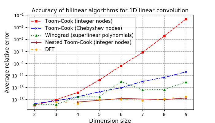
(a) 1D convolution

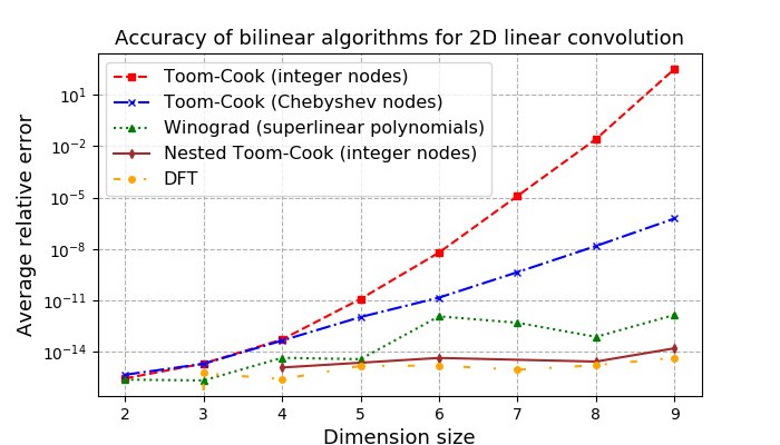
(b) 2D convolution

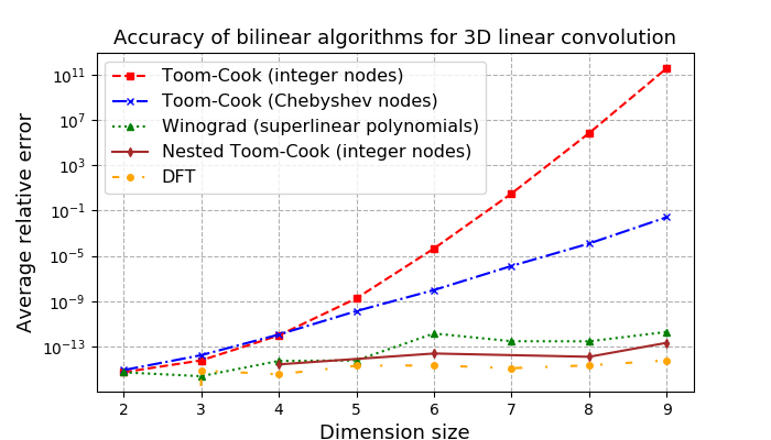
(c) 3D convolution

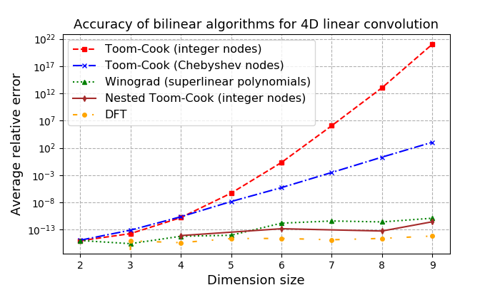
(d) 4D convolution

Figure 1: The relative error (averaged over ten trials) of the linear convolution between (random) $d$–dimensional tensors ($d=1,\ldots,4$) over various mode lengths ($n=2,\ldots,9$). For any dimension and mode length, the same pair of tensors were used in all convolution algorithms.

10.1 Accuracy of the Toom-Cook method

Figures 1(a), 1(b), 1(c), and 1(d) show the relative error of the Toom-Cook method using small integer and Chebyshev nodes. Both methods incur substantial errors when the input size exceeds size six, especially as the dimension of the problem increases. For multidimensional problems, the use of Chebyshev nodes can significantly reduce the relative error from using integer nodes. However, we observe that once the algorithm is used for 3D or 4D convolution with inputs greater than size seven, the use of Chebyshev nodes still leads to high errors.

10.2 Accuracy of the Winograd convolution algorithm

We implement Winograd’s convolution algorithm based on the formulation from Section 5 using the list of polynomial divisors $m^{(i)}$ from Table 4 and plot the average relative errors in Figs. 1(a), 1(b), 1(c), and 1(d). We observe that Winograd’s convolution algorithm with just one superlinear polynomial divisor (increasing rank by 1 with respect to optimum), as is the case for convolutions of size up to $6$, can significantly reduce the relative error compared to the Toom-Cook method with Chebyshev nodes. Furthermore, the number of flops required is only marginally larger than that of the Toom-Cook method. For a $5$-dimensional convolution, the number of additions, multiplications, and rank of Winograd’s convolution algorithm (Table 4) and the Toom-Cook method (Table 3) suggests that Winograd’s convolution algorithm can achieve highly accurate results without a significant increase in arithmetic or use of complex arithmetic as with the DFT.

10.3 Accuracy of the nested Toom-Cook method

We show the accuracy of the nested Toom-Cook method in Figs. 1(a), 1(b), 1(c), and 1(d). Like the Winograd convolution algorithm, this algorithm can significantly reduce the error of the Toom-Cook method. A downside to the nested Toom-Cook approach is that the bilinear rank is greatly increased as compared to Winograd’s convolution algorithm. For example, our implementation of a Winograd’s convolution algorithm for $8$-dimensional vectors has a rank of $17$, whereas the nested Toom-Cook algorithm has a bilinear rank of $27$.

However, a benefit of the nested Toom-Cook method is that the number of non–zeros in both the encoding and decoding matrices are lower than Winograd’s convolution algorithm, as shown seen in Table 5 and Table 4. For certain decompositions, the magnitude of the matrix elements never exceeds $1$, as these matrices are built from very small Toom-Cook methods. A nested Toom-Cook algorithm for $n=8$ can be created by a triply nested Toom-Cook algorithm for $n=2$, whose matrices are composed of zeros and the scalars $1$ and $1/2$ as well as their negatives. For convolutions where the overhead of applying the encoding and decoding is computationally expensive (such as near the leaves of the recursion tree), the nested Toom-Cook approach offers an accurate and efficient approach.

11 Future work

While novel strategies to reduce error from Section 9, such as better node points and diagonal scaling, have the potential to improve the accuracy of the convolution algorithm by a constant factor [6, 95], it remains an open question on how much these strategies can improve accuracy. A better understanding of the round-off error as well as finding an algorithm that determines the set of nodes and diagonal scaling with the optimal norm can help extend the use of Toom-Cook convolution algorithms to larger filter sizes. Similarly, there remains space for a more comprehensive search of divisor polynomials to produce encoding and decoding matrices with an optimal balance between sparsity, rank, and conditioning for the Winograd convolution algorithm. Experimental results suggest that polynomial divisors that are superlinear and added with positive/negative powers of two offer robust numerical accuracy [7]. Theory that supports this claim or finds other suitable polynomials can be of interest.

Furthermore, low–precision multipliers in deep neural networks are robust for both training and inferencing [23]. However, existing low–precision training strategies rely on high–precision convolutions or dot products. Especially with the emergence of mixed–precision training on accelerators such as Tensor Cores, deriving theoretical bounds as well as empirical results on the interplay between low–precision arithmetic and the accuracy of the various bilinear algorithms can be of interest to the deep learning and high–performance computing community.

Another area for future study is the design and analysis of fast parallel convolution algorithms. Performance of convolution algorithms in the parallel setting (such as on GPUs) is generally dominated by communication costs, i.e., the amount of data movement required to compute the algorithm. As the size of the dataset grows, more communication is needed. Demmel and Dinh derived communication lower bounds for the direct computation of the convolutional layer [26]. To extend their work, an open question is determining how much communication is needed for fast bilinear algorithms such as the Toom-Cook algorithm, Winograd’s convolution algorithm, and Toom-Cook with overlap-add. General approaches for deriving communication lower bounds of bilinear algorithms [88] may provide one avenue towards understanding communication costs in fast convolution algorithms. Moreover, a few of the convolution algorithms we consider (the one derived in Section 6.2 and the many–nested Toom-$2$ algorithm) can be formulated by taking products with sparse matrices. Exploration of efficient sparse linear algebra kernels for these convolution variants may yield convolution kernels with better performance and accuracy.

Another question is whether the interpolation and Winograd techniques covered in this paper encompass all possible fast bilinear algorithms for convolution. If these techniques do cover all possible fast bilinear algorithms, this knowledge can narrow the search for optimal bilinear algorithms in accuracy and number of flops.

12 Conclusion

Using the formalism of bilinear algorithms, we present different variants of convolution, including ones based on polynomial interpolation and modular polynomial arithmetic. We derive simple formulations for generating these bilinear algorithms. These explicit formulations allow us to quantify the cost of the various algorithms as well as simplify previous error bounds. Our analysis and experiments show that the nested convolution via overlap-add and Winograd’s convolution algorithm with superlinear polynomials can be effective for multidimensional convolution for a range of filter sizes. With the simplified construction of these convolution algorithms in the language of linear algebra, we hope researchers in scientific computing, applied mathematics, and machine learning can discover new uses and methods for fast convolution.

References

- [1] F. Adriaensen, Design of a convolution engine optimised for reverb, in LAC2006 Proceedings, 4th International Linux Audio Conference, Karlsruhe, 2006, pp. 49–53.
- [2] R. Agarwal and C. Burrus, Fast convolution using Fermat number transforms with applications to digital filtering, IEEE Transactions on Acoustics, Speech, and Signal Processing, 22 (1974), pp. 87–97.
- [3] R. Agarwal and J. Cooley, New algorithms for digital convolution, IEEE Transactions on Acoustics, Speech, and Signal Processing, 25 (1977), pp. 392–410.
- [4] T. Annala et al., Bézout’s theorem, (2016).
- [5] P. Balaprakash, R. Egele, M. Salim, S. Wild, V. Vishwanath, F. Xia, T. Brettin, and R. Stevens, Scalable reinforcement-learning-based neural architecture search for cancer deep learning research, in Proceedings of the International Conference for High Performance Computing, Networking, Storage and Analysis, 2019, pp. 1–33.
- [6] B. Barabasz, A. Anderson, and D. Gregg, Error analysis and improving the accuracy of Winograd convolution for deep neural networks, arXiv preprint arXiv:1803.10986, (2018).
- [7] B. Barabasz and D. Gregg, Winograd convolution for DNNs: Beyond linear polinomials, arXiv preprint arXiv:1905.05233, (2019).
- [8] G. Baszenski and M. Tasche, Fast polynomial multiplication and convolutions related to the discrete cosine transform, Linear Algebra and its Applications, 252 (1997), pp. 1–25.
- [9] R. R. Bitmead and B. D. Anderson, Asymptotically fast solution of Toeplitz and related systems of linear equations, Linear Algebra and its Applications, 34 (1980), pp. 103–116.
- [10] R. E. Blahut, Fast algorithms for signal processing, Cambridge University Press, 2010.
- [11] M. Bodrato, Towards optimal Toom-Cook multiplication for univariate and multivariate polynomials in characteristic 2 and 0, in International Workshop on the Arithmetic of Finite Fields, Springer, 2007, pp. 116–133.
- [12] A. Bojanczyk, R. Brent, and F. De Hoog, Qr factorization of Toeplitz matrices, Numerische Mathematik, 49 (1986), pp. 81–94.
- [13] A. Böttcher and S. M. Grudsky, Spectral properties of banded Toeplitz matrices, vol. 96, Siam, 2005.
- [14] A. F. Breitzman and J. R. Johnson, Automatic derivation and implementation of fast convolution algorithms, PhD thesis, Citeseer, 2003.
- [15] O. P. Bruno and L. A. Kunyansky, A fast, high-order algorithm for the solution of surface scattering problems: Basic implementation, tests, and applications, Journal of Computational Physics, 169 (2001), pp. 80 – 110, https://doi.org/https://doi.org/10.1006/jcph.2001.6714, http://www.sciencedirect.com/science/article/pii/S0021999101967142.
- [16] C. S. Burrus and T. W. Parks, DFT/FFT and Convolution Algorithms: Theory and Implementation, John Wiley & Sons, Inc., New York, NY, USA, 1st ed., 1991.
- [17] B. Chandrakar, O. Yadav, and V. Chandra, A survey of noise removal techniques for ECG signals, International Journal of Advanced Research in Computer and Communication Engineering, 2 (2013), pp. 1354–1357.
- [18] C. Cheng and K. K. Parhi, Hardware efficient fast parallel FIR filter structures based on iterated short convolution, IEEE Transactions on Circuits and Systems I: Regular Papers, 51 (2004), pp. 1492–1500.
- [19] Y. Cheng, D. Wang, P. Zhou, and T. Zhang, A survey of model compression and acceleration for deep neural networks, arXiv preprint arXiv:1710.09282, (2017).
- [20] S. Chetlur, C. Woolley, P. Vandermersch, J. Cohen, J. Tran, B. Catanzaro, and E. Shelhamer, CUDNN: Efficient primitives for deep learning, arXiv preprint arXiv:1410.0759, (2014).
- [21] J. Cong and B. Xiao, Minimizing computation in convolutional neural networks, in International conference on artificial neural networks, Springer, 2014, pp. 281–290.
- [22] S. A. Cook and S. O. Aanderaa, On the minimum computation time of functions, Transactions of the American Mathematical Society, 142 (1969), pp. 291–314.
- [23] M. Courbariaux, Y. Bengio, and J.-P. David, Training deep neural networks with low precision multiplications, arXiv preprint arXiv:1412.7024, (2014).
- [24] M. Courbariaux, J.-P. David, and Y. Bengio, Low precision storage for deep learning, arXiv preprint arXiv:1412.7024, (2014).
- [25] T. Darden, D. York, and L. Pedersen, Particle mesh Ewald: An method for Ewald sums in large systems, The Journal of chemical physics, 98 (1993), pp. 10089–10092.
- [26] J. Demmel and G. Dinh, Communication-optimal convolutional neural nets, arXiv preprint arXiv:1802.06905, (2018).
- [27] G. Deng and L. Cahill, An adaptive Gaussian filter for noise reduction and edge detection, in 1993 IEEE Conference Record Nuclear Science Symposium and Medical Imaging Conference, IEEE, 1993, pp. 1615–1619.
- [28] S. Dieleman, K. W. Willett, and J. Dambre, Rotation-invariant convolutional neural networks for galaxy morphology prediction, Monthly notices of the royal astronomical society, 450 (2015), pp. 1441–1459.
- [29] T. Elsken, J. H. Metzen, and F. Hutter, Neural architecture search: A survey, arXiv preprint arXiv:1808.05377, (2018).
- [30] Z. Fang, X. Li, and L. M. Ni, On the communication complexity of generalized 2-d convolution on array processors, IEEE Transactions on Computers, 38 (1989), pp. 184–194.
- [31] A. L. Fetter and J. D. Walecka, Quantum theory of many-particle systems, Courier Corporation, 2012.
- [32] O. Fialka and M. Cadik, FFT and convolution performance in image filtering on GPU, in Tenth International Conference on Information Visualisation (IV’06), IEEE, 2006, pp. 609–614.
- [33] B. Fischer and G. H. Golub, How to generate unknown orthogonal polynomials out of known orthogonal polynomials, Journal of Computational and Applied Mathematics, 43 (1992), pp. 99–115.
- [34] M. Frigo and S. G. Johnson, The design and implementation of FFTW3, Proceedings of the IEEE, 93 (2005), pp. 216–231.
- [35] W. Gautschi, How (un) stable are Vandermonde systems, Asymptotic and computational analysis, 124 (1990), pp. 193–210.
- [36] P. Getreuer, A survey of Gaussian convolution algorithms, Image Processing On Line, 2013 (2013), pp. 286–310.
- [37] B. Gold and K. Jordan, A direct search procedure for designing finite duration impulse response filters, IEEE Transactions on Audio and Electroacoustics, 17 (1969), pp. 33–36.
- [38] R. J. Harrison, G. I. Fann, T. Yanai, Z. Gan, and G. Beylkin, Multiresolution quantum chemistry: Basic theory and initial applications, The Journal of chemical physics, 121 (2004), pp. 11587–11598.
- [39] D. Harvey and J. Van Der Hoeven, Polynomial multiplication over finite fields in time , (2019).
- [40] D. Harvey, J. Van Der Hoeven, and G. Lecerf, Even faster integer multiplication, Journal of Complexity, 36 (2016), pp. 1–30.
- [41] K. He, X. Zhang, S. Ren, and J. Sun, Deep residual learning for image recognition, in Proceedings of the IEEE conference on computer vision and pattern recognition, 2016, pp. 770–778.
- [42] M. T. Heath, Scientific computing: an introductory survey, vol. 80, SIAM, 2018.
- [43] P. S. Heckbert, Survey of texture mapping, IEEE computer graphics and applications, 6 (1986), pp. 56–67.
- [44] M. T. Heideman and C. S. Burrus, Multiplicative complexity, convolution, and the DFT, Springer, 1988.
- [45] N. J. Higham, Accuracy and stability of numerical algorithms, vol. 80, Siam, 2002.
- [46] F. N. Iandola, S. Han, M. W. Moskewicz, K. Ashraf, W. J. Dally, and K. Keutzer, SqueezeNet: AlexNet-level accuracy with 50x fewer parameters and 0.5 MB model size, arXiv preprint arXiv:1602.07360, (2016).
- [47] F. N. Iandola, D. Sheffield, M. J. Anderson, P. M. Phothilimthana, and K. Keutzer, Communication-minimizing 2D convolution in GPU registers, in 2013 IEEE International Conference on Image Processing, IEEE, 2013, pp. 2116–2120.
- [48] N. Kanopoulos, N. Vasanthavada, and R. L. Baker, Design of an image edge detection filter using the Sobel operator, IEEE Journal of solid-state circuits, 23 (1988), pp. 358–367.
- [49] A. A. Karatsuba, The complexity of computations, Proceedings of the Steklov Institute of Mathematics-Interperiodica Translation, 211 (1995), pp. 169–183.
- [50] B. N. Khoromskij, On tensor approximation of Green iterations for Kohn-Sham equations, Computing and visualization in science, 11 (2008), pp. 259–271.
- [51] B. N. Khoromskij, Fast and accurate tensor approximation of a multivariate convolution with linear scaling in dimension, Journal of computational and applied mathematics, 234 (2010), pp. 3122–3139.
- [52] B. N. Khoromskij and V. Khoromskaia, Multigrid accelerated tensor approximation of function related multidimensional arrays, SIAM Journal on Scientific Computing, 31 (2009), pp. 3002–3026.
- [53] H. Kim, H. Nam, W. Jung, and J. Lee, Performance analysis of CNN frameworks for GPUs, in 2017 IEEE International Symposium on Performance Analysis of Systems and Software (ISPASS), IEEE, 2017, pp. 55–64.
- [54] T. G. Kolda and B. W. Bader, Tensor decompositions and applications. SIAM, 2009, https://epubs.siam.org/doi/abs/10.1137/07070111X.
- [55] R. Kress, V. Maz’ya, and V. Kozlov, Linear integral equations, vol. 82, Springer, 1989.
- [56] A. Krizhevsky, One weird trick for parallelizing convolutional neural networks, arXiv preprint arXiv:1404.5997, (2014).
- [57] A. Krizhevsky, I. Sutskever, and G. E. Hinton, Imagenet classification with deep convolutional neural networks, in Advances in neural information processing systems, 2012, pp. 1097–1105.
- [58] R. Kumar, A fast algorithm for solving a Toeplitz system of equations, IEEE transactions on acoustics, speech, and signal processing, 33 (1985), pp. 254–267.
- [59] V. Kumar and V. Purwar, FIR filter design using mixed algorithms: A survey, International Journal of Engineering and Technical Research, 7 (2017).
- [60] A. Lavin and S. Gray, Fast algorithms for convolutional neural networks, in Proceedings of the IEEE Conference on Computer Vision and Pattern Recognition, 2016, pp. 4013–4021.
- [61] Y. LeCun, L. Bottou, Y. Bengio, P. Haffner, et al., Gradient-based learning applied to document recognition, Proceedings of the IEEE, 86 (1998), pp. 2278–2324.
- [62] H. K. Lee, D. M. Higdon, C. A. Calder, and C. H. Holloman, Efficient models for correlated data via convolutions of intrinsic processes, Statistical Modelling, 5 (2005), pp. 53–74.
- [63] S. Lin and S. K. Mitra, Overlapped block digital filtering, IEEE Transactions on Circuits and Systems II: Analog and Digital Signal Processing, 43 (1996), pp. 586–596.
- [64] S. A. Martucci, Symmetric convolution and the discrete sine and cosine transforms, IEEE Transactions on Signal Processing, 42 (1994), pp. 1038–1051.
- [65] A. Mathuriya, D. Bard, P. Mendygral, L. Meadows, J. Arnemann, L. Shao, S. He, T. Kärnä, D. Moise, S. J. Pennycook, K. Maschhoff, J. Sewall, N. Kumar, S. Ho, M. F. Ringenburg, P. Prabhat, and V. Lee, CosmoFlow: Using deep learning to learn the Universe at scale, in SC18: International Conference for High Performance Computing, Networking, Storage and Analysis, Nov 2018, pp. 819–829, https://doi.org/10.1109/SC.2018.00068.
- [66] F. Milinazzo, C. Zala, and I. Barrodale, On the rate of growth of condition numbers for convolution matrices, IEEE Transactions on Acoustics, Speech, and Signal Processing, 35 (1987), pp. 471–475.
- [67] M. Mustafa, D. Bard, W. Bhimji, Z. Lukic, R. Al-Rfou, and J. M. Kratochvil, CosmoGAN: creating high-fidelity weak lensing convergence maps using generative adversarial networks, Computational Astrophysics and Cosmology, 6 (2019), p. 1, https://doi.org/10.1186/s40668-019-0029-9, https://doi.org/10.1186/s40668-019-0029-9.
- [68] M. J. Narasimha, Modified overlap-add and overlap-save convolution algorithms for real signals, IEEE Signal Processing Letters, 13 (2006), pp. 669–671.
- [69] H. V. Nguyen, E. Müller, J. Vreeken, P. Efros, and K. Böhm, Multivariate maximal correlation analysis, in International Conference on Machine Learning, 2014, pp. 775–783.
- [70] H. J. Nussbaumer, Fast Fourier transform and convolution algorithms, vol. 2, Springer Science & Business Media, 2012.
- [71] V. Pan, How can we speed up matrix multiplication?, SIAM review, 26 (1984), pp. 393–415.
- [72] V. Y. Pan, Structured matrices and polynomials: unified superfast algorithms, Springer Science & Business Media, 2012.
- [73] V. Y. Pan, How bad are Vandermonde matrices?, SIAM Journal on Matrix Analysis and Applications, 37 (2016), pp. 676–694.
- [74] K. Pavel and S. David, Algorithms for efficient computation of convolution, Design and Architectures for Digital Signal Processing, (2013), pp. 179–208.
- [75] B. G. Pierce, Y. Hourai, and Z. Weng, Accelerating protein docking in zdock using an advanced 3d convolution library, PloS one, 6 (2011).
- [76] A. Podili, C. Zhang, and V. Prasanna, Fast and efficient implementation of convolutional neural networks on FPGA, in 2017 IEEE 28th International Conference on Application-specific Systems, Architectures and Processors (ASAP), IEEE, 2017, pp. 11–18.
- [77] W. K. Pratt, Correlation techniques of image registration, IEEE transactions on Aerospace and Electronic Systems, (1974), pp. 353–358.
- [78] C. Quate and R. Thompson, Convolution and correlation in real time with nonlinear acoustics, Applied Physics Letters, 16 (1970), pp. 494–496.
- [79] R. Rice, Inverse convolution filters, Geophysics, 27 (1962), pp. 4–18.
- [80] S. Sakthikumaran, S. Salivahanan, and V. K. Bhaaskaran, 16-bit RISC processor design for convolution application, in 2011 International Conference on Recent Trends in Information Technology (ICRTIT), IEEE, 2011, pp. 394–397.
- [81] V. Sandhiya, S. Karthick, and M. Valarmathy, A survey of new reconfigurable architectures for implementing FIR filters with low complexity, in 2014 International Conference on Computer Communication and Informatics, IEEE, 2014, pp. 1–9.
- [82] J. Schmelzle, A. Lucchi, T. Kacprzak, A. Amara, R. Sgier, A. Réfrégier, and T. Hofmann, Cosmological model discrimination with Deep Learning, (2017), https://arxiv.org/abs/1707.05167.
- [83] A. Schönhage and V. Strassen, Schnelle Multiplikation grosser Zahlen, Computing, 7 (1971), pp. 281–292.
- [84] I. W. Selesnick and C. S. Burrus, Extending Winograd’s small convolution algorithm to longer lengths, in Proceedings of IEEE International Symposium on Circuits and Systems-ISCAS’94, vol. 2, IEEE, 1994, pp. 449–452.
- [85] I. W. Selesnick and C. S. Burrus, Fast convolution and filtering, 1998.
- [86] N. D. Sidiropoulos, L. De Lathauwer, X. Fu, K. Huang, E. E. Papalexakis, and C. Faloutsos, Tensor decomposition for signal processing and machine learning, IEEE Transactions on Signal Processing, 65 (2017), pp. 3551–3582.
- [87] E. Solomonik and J. Demmel, Contracting symmetric tensors using fewer multiplications, tech. report, ETH Zurich, 2015, https://doi.org/http://dx.doi.org/10.3929/ethz-a-010345741.
- [88] E. Solomonik, J. Demmel, and T. Hoefler, Communication lower bounds for tensor contraction algorithms, tech. report, ETH Zurich, 2015, https://doi.org/http://dx.doi.org/10.3929/ethz-a-010350411.
- [89] G. Strang, The discrete cosine transform, SIAM review, 41 (1999), pp. 135–147.
- [90] V. Strassen, Gaussian elimination is not optimal, Numerische Mathematik, 13 (1969), pp. 354–356, https://doi.org/10.1007/BF02165411, http://dx.doi.org/10.1007/BF02165411.
- [91] C. Szegedy, W. Liu, Y. Jia, P. Sermanet, S. Reed, D. Anguelov, D. Erhan, V. Vanhoucke, and A. Rabinovich, Going deeper with convolutions, in Proceedings of the IEEE conference on computer vision and pattern recognition, 2015, pp. 1–9.
- [92] R. Takapoui and H. Javadi, Preconditioning via diagonal scaling, arXiv preprint arXiv:1610.03871, (2016).
- [93] R. Tolimieri, M. An, and C. Lu, Algorithms for Discrete Fourier Transform and Convolution, Springer New York, 1989, https://doi.org/10.1007/978-1-4757-3854-4, https://doi.org/10.1007%2F978-1-4757-3854-4.
- [94] A. L. Toom, The complexity of a scheme of functional elements realizing the multiplication of integers, in Soviet Mathematics Doklady, vol. 3, 1963, pp. 714–716.
- [95] K. Vincent, K. Stephano, M. Frumkin, B. Ginsburg, and J. Demouth, On improving the numerical stability of Winograd convolutions, (2017).
- [96] G. Wei, Discrete singular convolution for the solution of the Fokker–Planck equation, The Journal of chemical physics, 110 (1999), pp. 8930–8942.
- [97] S. Winograd, Arithmetic complexity of computations, vol. 33, Siam, 1980.
- [98] S. Yang, Y. Zhou, and G. Wei, Comparison of the discrete singular convolution algorithm and the Fourier pseudospectral method for solving partial differential equations, Computer Physics Communications, 143 (2002), pp. 113–135.
- [99] K. Ye and L.-H. Lim, Every matrix is a product of Toeplitz matrices, Foundations of Computational Mathematics, 16 (2016), pp. 577–598.
- [100] Y. You, J. Hseu, C. Ying, J. Demmel, K. Keutzer, and C.-J. Hsieh, Large-batch training for lstm and beyond, in Proceedings of the International Conference for High Performance Computing, Networking, Storage and Analysis, 2019, pp. 1–16.
- [101] A. Zanoni, Iterative Toom-Cook methods for very unbalanced long integer multiplication, in Proceedings of the 2010 International Symposium on Symbolic and Algebraic Computation, ACM, 2010, pp. 319–323.
- [102] M. D. Zeiler and R. Fergus, Visualizing and understanding convolutional networks, in European conference on computer vision, Springer, 2014, pp. 818–833.
- [103] A. Zlateski, Z. Jia, K. Li, and F. Durand, FFT convolutions are faster than Winograd on modern CPUs, here is why, arXiv preprint arXiv:1809.07851, (2018).