Voronoï tesselation analysis of sets of randomly placed finite-size spheres

Abstract

The purpose of this note is to clarify the effect of the finite size of spherical particles upon the characteristics of their spatial distribution through a random Poisson process (RPP). This information is of special interest when using RPP data as a reference for the analysis of the spatial structure of a given (non-RPP) particulate system, in which case ignoring finite-size effects upon the former may yield misleading conclusions. We perform Monte Carlo simulations in triply-periodic spatial domains, and then analyze the particle-centered Voronoï tesselations for solid volume fractions ranging from $10^{-5}$ to $0.3$. We show that the standard-deviation of these volumes decreases with the solid volume fraction, the deviation from the value of point sets being reasonably approximated by an exponential function. As can be expected, the domain size for which the random assemblies of finite-size particles are generated has a constraining effect if the number of particles per realization is chosen too small. This effect is quantified, and recommendations are given. We have also revisited the case of random point sets (i.e. the limit of vanishing particle diameter), for which we have confirmed the accuracy of the earlier data by Tanemura [Forma, 18(4):221–247, 2003].

1 Introduction

One method to characterize the spatial distribution of particles is with the help of Voronoï tesselation. As initially proposed in the context of particulate multi-phase flow by Monchaux et al. (2010) and further elaborated by Monchaux et al. (2012), such a tesselaton can give valuable information on the tendency of particles to cluster. Apart from partitioning space and therefore allowing for an interpretation as the inverse of a local concentration, the tesselation further generates data on the connectivity (“neighborhood”) between particles, and it can therefore be directly used for the purpose of cluster identification and for quantifying Lagrangian aspects of clustering. Another benefit is the intrinsic definition of a clustering threshold (Monchaux et al., 2010) without the need for a priori selection of a length-scale. A further important advantage is the availability of a fast algorithm for performing the tesselation (in the present note we either use the Matlab implementation of the “QHULL” library, Barber et al. 1996, or the “VORO++” library, Rycroft 2009, both of which provide a scaling of the execution time which is linear in the number of particles). For these reasons, various analysis methods based upon Voronoï tesselation of particle positions have found relatively wide-spread use in the particulate flow community (Obligado et al., 2011; García-Villalba et al., 2012; Fiabane et al., 2012; Tagawa et al., 2012; Dejoan and Monchaux, 2013; Kidanemariam et al., 2013; Uhlmann and Doychev, 2014; Sumbekova et al., 2016; Uhlmann and Chouippe, 2017; Monchaux and Dejoan, 2017; Chouippe and Uhlmann, 2018).

The usual procedure in most of these afore-mentioned studies consists in comparing the statistics of the actual particle distributions in the respecitve multiphase flow systems (either obtained from experimental measurements or from numerical simulations) with data for particle distributions obtained by a random Poisson process (henceforth denoted as “RPP”), i.e. drawing them randomly from a distribution which is uniform in space. Statistically significant differences are then a sign of “structure” in the particle set, and these features can subsequently be interpreted on physical grounds.

The spatial distribution of a set of points through an RPP has been investigated in the literature (Tanemura, 2003; Ferenc and Neda, 2007, and references therein). Although no analytical results are available, these authors have proposed empirical fits for the probability distribution of the Voronoï cell volumes as well as providing reference values for the first few moments which are widely used. In some applications the shape of the probability density function (pdf) of Voronoï cell volumes does not change much, which means that the data is reasonably described by a single parameter, i.e. the second moment. It is then common practice to use the difference between the measured standard deviation and the literature value of an RPP-generated set of points as a proxy for the tendency to cluster (Monchaux et al., 2010).

Due to the finite size of real-world particles, theoretical results derived for the spatial distribution of points (such as those given by Ferenc and Neda, 2007) do no longer strictly apply. This is due to the fact that there exists a lower bound for the closest packing of finite-size particles as they cannot overlap. This aspect as well as the impact of a finite domain size (both in numerical simulations and in laboratory-experimental measurements) has so far not been systematically documented. Oger et al. (1996) have observed that the probability distribution of Voronoï cell volumes changes from a Gamma distribution to a Gaussian when going from one extreme in terms of the solid volume fraction to the other (i.e. from a point set to a close sphere packing).

Incidentally, let us note that Tagawa et al. (2012) have reported on the effect of the number of particle samples upon the standard deviation of Voronoï cell volumes determined for numerical data-sets of point particles. Monchaux (2012) have analyzed biases in Voronoï-based analysis of experimental data, focusing on: (i) the effect of projecting onto two spatial dimensions from measurements with a laser sheet with non-vanishing thickness; (ii) sub-sampling due to “missed” particles; (iii) slight polydispersity.

In the present note we first revisit the case of point sets, before addressing the following questions pertaining to the statistics of spherically-shaped particles distributed through a random Poisson process: what is the effect of a non-vanishing particle size? What is the effect of a finite solid volume fraction? What is the influence of the relative domain size?

2 Revisiting the results for sets of points

We consider the case of $N_{p}$ points distributed inside of a cubical domain of side-length $L$. For the sake of generality, we consider $N_{s}$ independently drawn such distributions (i.e. snapshots). Since there is no second length-scale, the problem is then completely determined by the two non-dimensional numbers $N_{p}$ and $N_{s}$.

The Voronoï tesselation is performed by assuming periodicity of the field over all three spatial directions. This can be (naively) implemented algorithmically by (redundant) periodic extension of the fields and later eliminating the duplicate cells on the borders of the fundamental domain.

$(a)$

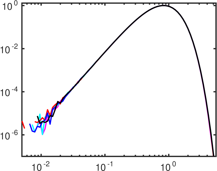
$V_{vor}/\langle V\rangle$

pdf

pdf

$(b)$

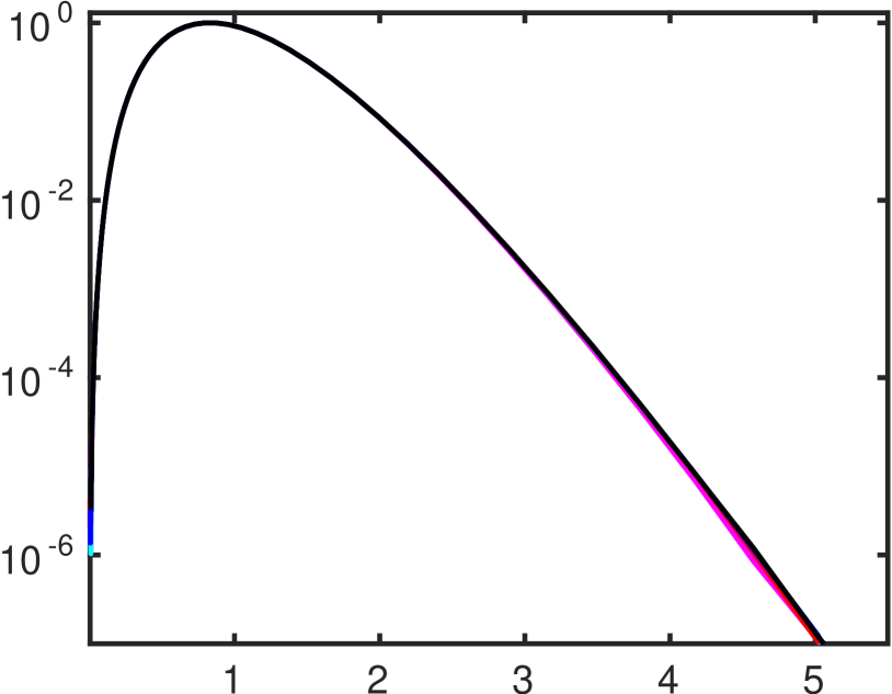
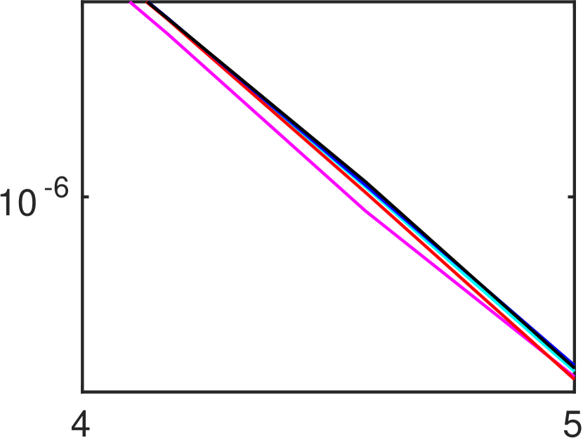
$V_{vor}/\langle V\rangle$

Figure 1: Probability density function of the volume of Voronoï cells for sets of points distributed according to an RPP. The number of points per snapshot is indicated by the colors as follows:  , $N_{p}=10^{7}$;  , $N_{p}=10^{6}$;  , $N_{p}=10^{5}$;  , $N_{p}=10^{4}$;  , $N_{p}=10^{3}$; The total number of samples is kept constant ($N_{tot}=N_{p}\,N_{s}=5\cdot 10^{9}$) in the entire series by adjusting the number of snapshots $N_{s}$ accordingly. Graph $(a)$ shows double logarithmic scaling; $(b)$ is the same data in semi-logarithmic scaling. The inset shows a zoom of the right tail.

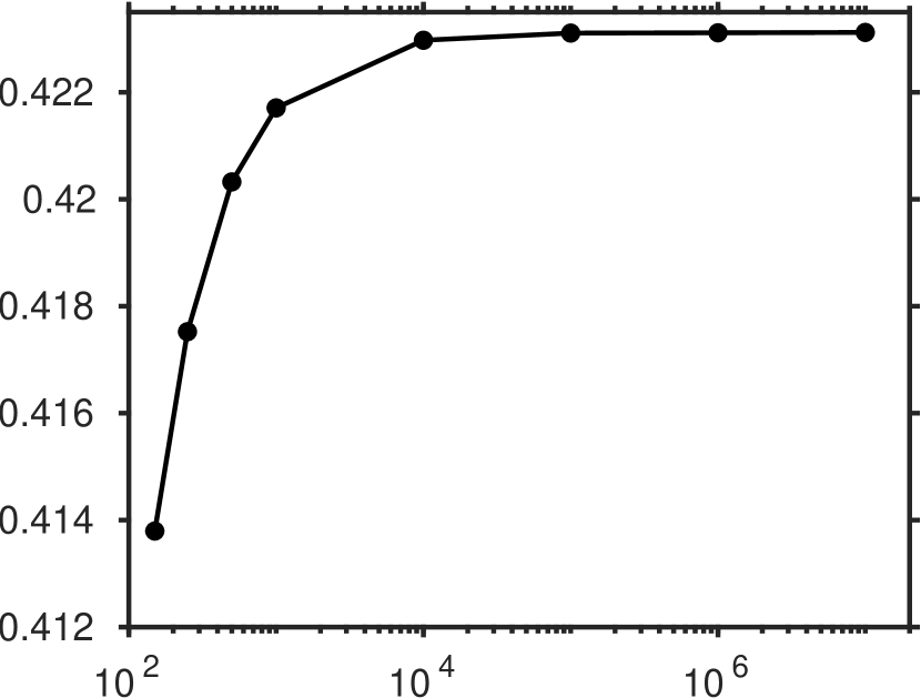
$N_{p}$

$\sigma(V_{vor}/\langle V\rangle)$

Figure 2: Standard deviation of the volume of Voronoï cells for sets of points distributed according to an RPP, shown as a function of the number of particles $N_{p}$ per snapshot. The total number of samples is kept constant ($N_{tot}=N_{p}\,N_{s}=5\cdot 10^{9}$) in the entire series by adjusting the number of snapshots $N_{s}$ accordingly.

$(a)$

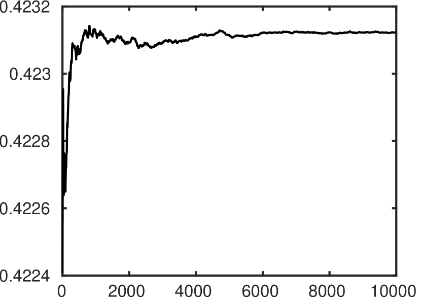
$N_{s}$

$\sigma(N_{s})$

$(\sigma(N_{s})-\sigma(10^{4}))/\sigma(10^{4})$

$(b)$

$N_{s}$

Figure 3: Convergence of the standard deviation of the volume of Voronoï cells for sets of points distributed according to an RPP, shown as a function of the number of snapshots $N_{s}$, for $N_{p}=10^{5}$. $(a)$ running average; $(b)$ relative error with respect to the value obtained for the entire sequence.

Figure 1 shows the probibility density function obtained by numerical experiments with $N_{tot}=N_{p}\,N_{s}=5\cdot 10^{9}$ samples, by varying the number of particles per snapshot in the range $N_{p}=10^{3}\ldots 10^{7}$ and adjusting the number of snapshots $N_{s}$ accordingly. It can be seen that the differences are marginal. The pdf can be fitted to a three-parameter (generalized) Gamma distribution, viz.

$$f(x)=\frac{c\,b^{a/c}}{\Gamma(a/c)}x^{a-1}\exp(-b\,x^{c})\,,$$ (1)

with the following set of coefficients borne out by our data with $N_{p}=10^{7}$ and $N_{s}=500$:

$$a=4.806\,,\quad b=4.045\,,\quad c=1.168\,.$$ (2)

These values are very close to those determined by Tanemura (2003) who proposes $a=4.798$. $b=4.040$, $c=1.168$; they are somewhat distinct from those obtained by Ferenc and Neda (2007). Figure 2 shows the influence of the number of points per snapshot upon the standard-deviation of the Voronoï cell volumes. It can be seen that the influence becomes insignificant for $N_{p}\geq 10^{4}$ particles. For smaller numbers, it turns out that the standard-deviation is underpredicted. This is due to the small deviations in the right tails (for large cell volumes) which are visible in the insert of figure 1$(b)$. The differences are presumably caused by an under-representation of very large cell volumes in ensembles with smaller numbers of particles.

Let us briefly mention the convergence of the second moment with the number of samples $N_{s}$. Figure 3 exemplarily shows the data for the case with $N_{p}=10^{5}$. Convergence is obviously not regular (since there is no order in the sequence), and, therefore, it needs to be monitored in practice.

As a bottom line, we state our best approximation of the standard-deviation of Voronoï cell volumes for sets of points drawn according to an RPP as follows:

$$\sigma(V_{vor}/\langle V\rangle)=0.42312\,.$$ (3)

3 Sets of finite-size particles

Now let us turn to the case of a distribution of a set of $N_{p}$ spherical, mono-dispersed particles with diameter $D$, again placed by means of an RPP in a cubical box of side-length $L$. Each draw of particle positions is done through a simple Monte Carlo method (Owen, 2013), performed under the constraint that no two particles should overlap. This is performed for each set by first drawing individual particle positions sequentially from a uniform and independent probability distribution (as in the case of sets of points treated above), testing each new candidate for geometrical overlap with all previously determined positions in the set, and, if overlap is found, discarding that candidate, then re-drawing, and so on until no overlap is detected (cf. algorithm 1). The present procedure is equivalent to random sequential addition (RSA) of hard spheres, as sometimes used in the context of physical chemistry in order to obtain random sphere arrangements (Widom, 1966). In particular, it has been shown that RSA leads to a so-called jamming limit (i.e. an upper bound for the solid volume fraction $\Phi_{s}$ where no additional spheres can be placed without overlapping) for $\Phi_{s}^{(RSA)}\approx 0.382$ (Talbot et al., 1991). Note that the RSA limit is significantly lower than the densest possible sphere packing ($\Phi_{s}^{(densest)}\approx 0.74$). In the present work we have considered solid volume fractions up to $0.3$; for values which are even closer to $\Phi_{s}^{(RSA)}$ it becomes challenging to determine a sufficiently large number $N_{s}$ of particle assemblies, since the required number of draws $N_{draws}$ in algorithm 1 eventually increases exponentially with $\Phi_{s}$.

Algorithm 1 Determines a single snapshot, i.e. a spatial distribution of $N_{p}$ finite-size particles which do not overlap. The number of required draws is stored in the variable $N_{draws}$.

$N_{draws}=0$

for $i=1\ldots N_{p}$ do $\triangleright$ loop over particle set

     redraw=true

     while redraw do

         draw ${X}^{(i)}_{\alpha}$ from uniform distribution $\forall\,\alpha=1,2,3$

         $N_{draws}\leftarrow N_{draws}+1$

         if $\mathbf{X}^{(i)}$ does not lead to overlap with any particle $j=1\ldots i-1$ then

              redraw=false

         end if

     end while

end for

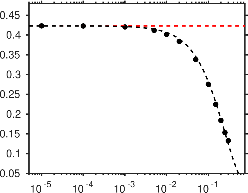
$\Phi_{s}=0$ (points)

$\Phi_{s}$

$\sigma(V_{vor}/\langle V\rangle)$

Figure 4: Standard deviation of the volume of Voronoï cells for $N_{p}=10^{5}$ finite-size particles distributed according to an RPP, as a function of the solid volume fraction $\Phi_{s}$. The ratio of box-size to particle diameter was varied accordingly, i.e. $L/D=(N_{p}\pi/(6\Phi_{s}))^{1/3}$. The number of snapshots analyzed in each case was $N_{s}=2000$, such that the total number of samples for each data point measures $N_{tot}=2\cdot 10^{8}$. Included is the value $\sigma(\Phi_{s}=0)$ for an RPP distribution of points, as given in (3). The black dashed line indicates the exponential fit (5).

Here the relevant variables are $N_{p}$ (number of particles in the set), $N_{s}$ (number of particle assemblies analyzed), $D$ (particle diameter) and $L$ (edge length of the computational cube), which leads to similarity under three non-dimensional parameters. Those can be chosen as: $N_{p}$, $N_{s}$ and $L/D$. Alternatively, one can use the solid volume fraction

$$\Phi_{s}=\frac{\pi}{6}\,N_{p}\,\left(\frac{D}{L}\right)^{3}\,,$$ (4)

for the characterisation of a parameter point (instead of either $N_{p}$ or $L/D$), and/or the total number of samples $N_{tot}=N_{p}N_{s}$.

3.1 Influence of solid volume fraction

In a first series we vary the solid volume fraction $\Phi_{s}$, while keeping the number of particles per snapshot constant at $N_{p}=10^{5}$, i.e. varying the ratio of box-size to particle diameter accordingly, and systematically using a number of $N_{s}=2000$ snapshots ($N_{tot}=2\cdot 10^{8}$). Figure 4 shows the progressive deviation of the standard-deviation of Voronoï cell volumes from the point-set value with increasing solid volume fraction. This deviation can be reasonably fitted with the aid of an exponential function in $\Phi_{s}$, viz.

$$\sigma(V_{vor}/\langle V\rangle)=\sigma(\Phi_{s}=0)\cdot\exp\left(-4.07\Phi_{s}\right)\,,$$ (5)

which might be useful as an approximation.

$(a)$

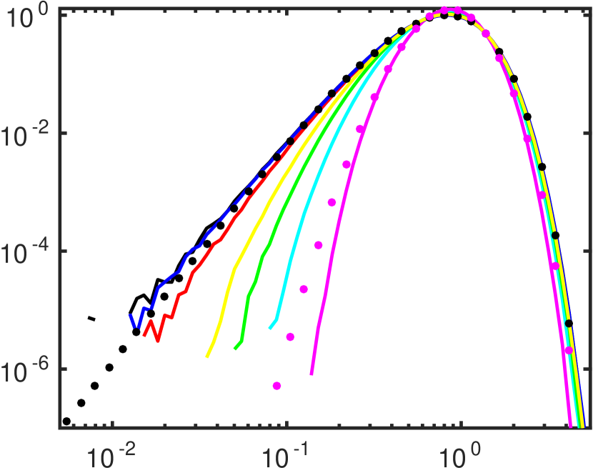
$V_{vor}/\langle V\rangle$

pdf

pdf

$(b)$

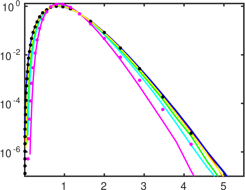
$V_{vor}/\langle V\rangle$

Figure 5: Probability density function of the volume of Voronoï cells for sets of spherical, finite-size particles distributed according to an RPP, shown for the data of figure 4. The line-styles are as follows:  , $\Phi_{s}=10^{-5}$;  , $\Phi_{s}=10^{-4}$;  , $\Phi_{s}=10^{-3}$;  , $\Phi_{s}=5\cdot 10^{-3}$;  , $\Phi_{s}=10^{-2}$;  , $\Phi_{s}=2\cdot 10^{-2}$;  , $\Phi_{s}=5\cdot 10^{-2}$. Graph $(a)$ shows double logarithmic scaling; $(b)$ is the same data in semi-logarithmic scaling. The solid circles indicate the respective fits to a generalized gamma distribution (1) for the most dilute and the densest cases.

The corresponding probability density functions of Voronoï cell volumes for these Monte Carlo experiments are shown in figure 5. They can again be fitted reasonably well to three-parameter (generalized) gamma distributions (1), with the shape morphing from the parameter set ($a=4.81$, $b=4.05$, $c=1.17$) for $\Phi_{s}=10^{-5}$ (i.e. practically identical to the point-set, given in 2) to ($a=16.37$, $b=31.73$, $c=0.52$) for $\Phi_{s}=5\cdot 10^{-2}$. Note from (4) that the solid volume fraction is equal to the ratio between the volume occupied by a particle and the mean volume of the Voronoï cells, i.e. $\Phi_{s}=V_{p}/\langle V_{vor}\rangle$, where $V_{p}=D^{3}\pi/6$. Since for non-overlapping particles a Voronoï cell cannot be smaller than the volume occupied by the particle itself, $min(V_{vor})\leq V_{p}$, it follows that a lower bound on the normalized Voronoï cell volumes is given by the solid volume fraction itself, viz. $min(V_{vor})/\langle V_{vor}\rangle\leq\Phi_{s}$. This lower bound is consistent with what can be observed in the progressive disappearance of the left tails in figure 5$(a)$. As a consequence of conservation of total volume, the probability of finding large cells correspondingly decreases, i.e. the right tails are likewise reduced (cf. figure 5$b$).

$(a)$

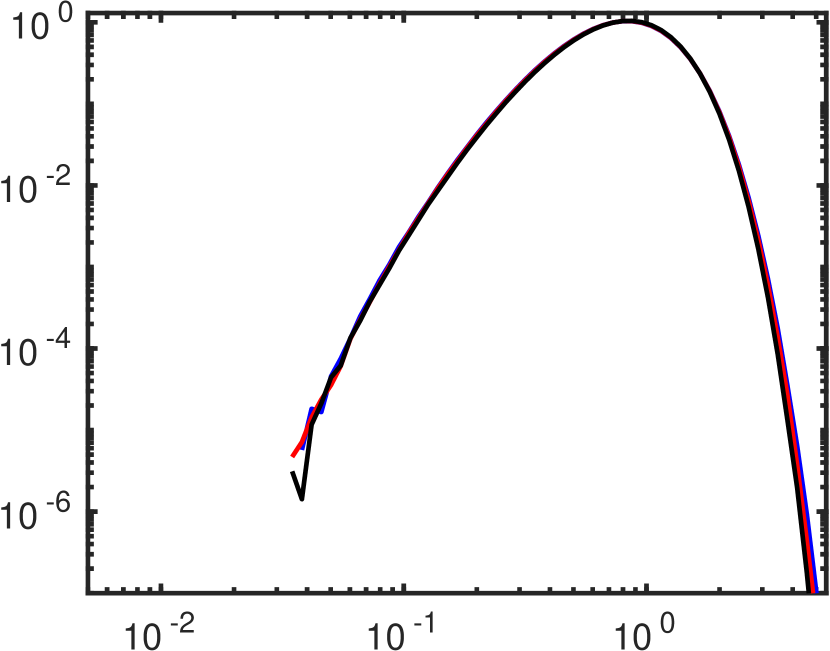
$V_{vor}/\langle V\rangle$

pdf

pdf

$(b)$

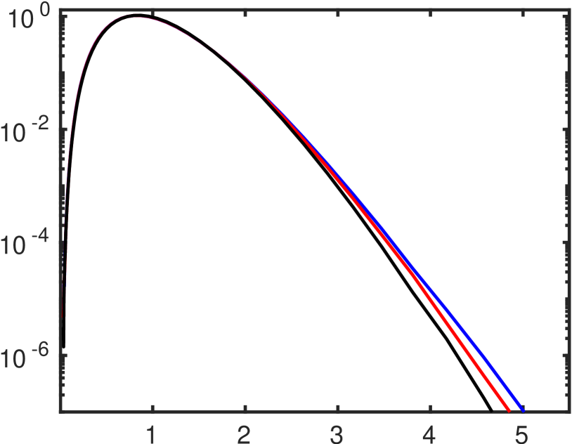
$V_{vor}/\langle V\rangle$

Figure 6: Probability density function of the volume of Voronoï cells for sets of finite-size particles with solid volume fraction $\Phi_{s}=5\cdot 10^{-3}$, distributed according to an RPP. The relative box-size is indicated by the colors as follows:  , $L/D=25$;  , $L/D=35$;  , $L/D=150$. Graph $(a)$ shows double logarithmic scaling; $(b)$ is the same data in semi-logarithmic scaling.

3.2 Influence of box size

Here we first fix a value for the solid volume fraction $\Phi_{s}$. We then perform simple Monte Carlo simulations for parameter points featuring distinct values of the length-scale ratio $L/D$. This means that for each parameter pair $(\Phi_{s},L/D)$ the number of particles per realization is different, i.e. $N_{p}=\Phi_{s}(\pi/6)(L/D)^{3}$. Again we adjust the overall number of samples per parameter point $(N_{tot}=N_{p}N_{s}$) by adapting the number of snapshots $N_{s}$; for this series we use $N_{tot}\geq 2\cdot 10^{8}$.

It can be seen from the pdfs shown in figure 6 that the smallest box-sizes lead to constraints which are particularly visible in the far right tails of the distribution (i.e. the probability of finding very large Voronoï cells is progressively reduced). Figure 7 then shows that the box-size effect upon the standard deviation is rather mild as compared to the effect of the solid volume fraction analyzed in § 3.1. A significant influence only starts to be noticeable for very small relative sizes of the spatial domains $L/D$. It can be seen in the figure that the value of $L/D$ at which the domain becomes “small” depends upon the solid volume fraction. In figure 8 we have normalized the data by its asymptotic value for large domains (denoted as $V_{vor}/\langle V\rangle^{\ast}$). As expected, the curves for the two different solid volume fractions collapse up to statistical uncertainty; they also collapse with the normalized curve for the point-set. We can then see that “small” simply means that the number of particles is below a certain threshold, say $N_{p}\leq 10^{4}$.

This threshold can also be argued via a detour, defining a critical length-scale ratio $(L/\ell)_{crit}$ below which the domain can be considered as “small” (here “$\ell$” stands for a characteristic length scale of the random particle arrangement). Let us assume that the characteristic length can be defined from the mean cell volume of a Voronoï cell, viz. $\ell=\langle V_{vor}\rangle^{1/3}$. Then, from the definition $\langle V_{vor}\rangle=L^{3}/N_{p}$ it directly follows that $L/\ell=N_{p}^{1/3}$, indicating that the critical value will only depend upon the number of particles, as indeed observed in figure 8.

$(a)$

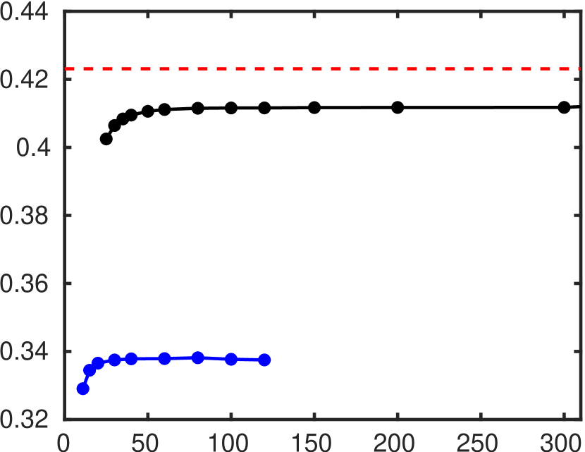
$\Phi_{s}=0$ (points)                         $\Phi_{s}=0.005$ $\Phi_{s}=0.05$

$L/D$

$\sigma(V_{vor}/\langle V\rangle)$

$\sigma(V_{vor}/\langle V\rangle)$

$(b)$

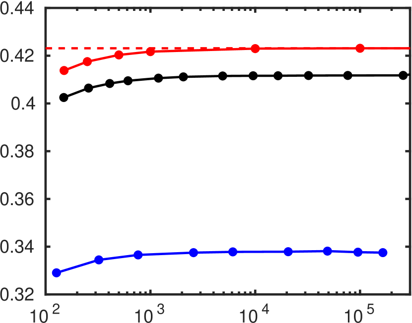
$\Phi_{s}=0$ $\Phi_{s}=0.005$ $\Phi_{s}=0.05$

$N_{p}$

Figure 7: Standard deviation of the volume of Voronoï cells for finite-size particles distributed in space according to an RPP, shown as: $(a)$ a function of the relative box-size $L/D$; $(b)$ a function of the number of particles per box $N_{p}$. Each line corresponds to a different value of the solid volume fraction, as indicated. The open symbols in blue color in graph $(b)$ correspond to the point-particle data of figure 2.

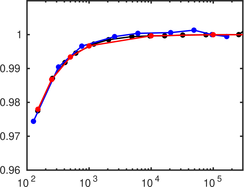
$N_{p}$

$\sigma(V_{vor}/\langle V\rangle)/\sigma(V_{vor}/\langle V\rangle)^{\ast}$

Figure 8: The same data as in figure 7$(b)$, but the ordinate is normalized with the asymptotic value of $\sigma(V_{vor}/\langle V\rangle)$ for large $N_{p}$. The line-styles are as follows:  , $\Phi_{s}=0$ (points);  , $\Phi_{s}=5\cdot 10^{-3}$;  , $\Phi_{s}=5\cdot 10^{-2}$.

4 Conclusions

We have investigated random arrangements of point sets and of non-overlapping, finite-size particles in cubical domains assumed to be tri-periodic. The analysis was performed with the aid of Voronoï tesselation, a tool which is frequently employed in the context of particulate flow and other branches of natural sciences and engineering. With this study we have addressed several aspects that have previously not been documented in a systematic way.

First, we have revisited the case of point sets. It was shown that the statistics of a random arrangement (assigned through a random Poisson process, RPP, which was repeated $N_{s}$ times per parameter point) depend upon the number of particles $N_{p}$, even if the total number of samples (i.e. the product $N_{p}N_{s}$) is sufficiently large. Our present data leads to the following best fit to a generalized three-parameter Gamma distribution (1):

$$a=4.806\,,\quad b=4.045\,,\quad c=1.168\,,$$

which yields as value for the standard deviation:

$$\sigma(V_{vor}/\langle V\rangle)=0.42312\,.$$

This value is very close to the result stated by Tanemura (2003), while if differs by roughly 3% from the result of Ferenc and Neda (2007).

Second, we have analyzed spatial arrangements of finite-size, spherical particles generated through an RPP. The problem depends upon two non-dimensional parameters (apart from the total number of samples $N_{p}N_{s}$): the solid volume fraction and the relative domain size. Through numerical evaluation it is demonstrated that the influence of the solid volume fraction $\Phi_{s}$ upon the standard deviation of the Voronoï cell volumes can be very significant, with the deviation from the value for a point-set increasing exponentially with $\Phi_{s}$ over the investigated range of $10^{-5}$ to $0.3$. An approximation which might be useful in practical applications is provided in equation (5).

Concerning the box-size dependence, it is found that – as expected – the low-order statistics of the tesselation are constrained if the box-size is below a certain threshold value. This threshold is independent of the solid volume fraction if expressed in terms of the number of particles per realization. If a number $N_{p}\geq 10^{4}$ is chosen, the relative deviation is kept below $3\cdot 10^{-4}$.

References

- Monchaux et al. (2010) R. Monchaux, M. Bourgoin, and A. Cartellier. Preferential concentration of heavy particles: A Voronoï analysis. Phys. Fluids, 22:103304, 2010. doi:10.1063/1.3489987.
- Monchaux et al. (2012) R. Monchaux, M. Bourgoin, and A. Cartellier. Analyzing preferential concentration and clustering of inertial particles in turbulence. Int. J. Multiphase Flow, 40:1–18, 2012. doi:10.1016/j.ijmultiphaseflow.2011.12.001.
- Barber et al. (1996) C.B. Barber, D.P. Dobkin, and H. Huhdanpaa. The quickhull algorithm for convex hulls. ACM Trans. Math. Softw., 22(4):469–483, December 1996. doi:10.1145/235815.235821.
- Rycroft (2009) C.H. Rycroft. Voro++: A three-dimensional Voronoi cell library in C++. Chaos, 19(4):041111, 2009. doi:10.1063/1.3215722.
- Obligado et al. (2011) M. Obligado, M. Missaoui, R. Monchaux, A. Cartellier, and M. Bourgoin. Reynolds number influence on preferential concentration of heavy particles in turbulent flows. J. Phys.: Conference Series, 318(5):052015, dec 2011. doi:10.1088/1742-6596/318/5/052015.
- García-Villalba et al. (2012) M. García-Villalba, A.G. Kidanemariam, and M. Uhlmann. DNS of vertical plane channel flow with finite-size particles: Voronoi analysis, acceleration statistics and particle-conditioned averaging. Int. J. Multiphase Flow, 46:54–74, 2012. doi:10.1016/j.ijmultiphaseflow.2012.05.007.
- Fiabane et al. (2012) L. Fiabane, R. Zimmermann, R. Volk, J.-F. Pinton, and M. Bourgoin. Clustering of finite-size particles in turbulence. Phys. Rev. E, 86(035301(R)), 2012. doi:10.1103/PhysRevE.86.035301.
- Tagawa et al. (2012) Y. Tagawa, J Martinez-Mercado, V.N. Prakash, E. Calzavarini, C. Sun, and D. Lohse. Three-dimensional Lagrangian Voronoï analysis for clustering of particles and bubbles in turbulence. J. Fluid Mech., 693:201–215, 2012. doi:10.1017/jfm.2011.510.
- Dejoan and Monchaux (2013) A. Dejoan and R. Monchaux. Preferential concentration and settling of heavy particles in homogeneous turbulence. Phys. Fluids, 25(1):013301, 2013. doi:10.1063/1.4774339.
- Kidanemariam et al. (2013) A.G. Kidanemariam, C. Chan-Braun, T. Doychev, and M. Uhlmann. DNS of horizontal open channel flow with finite-size, heavy particles at low solid volume fraction. New J. Phys., 15(2):025031, 2013. doi:10.1088/1367-2630/15/2/025031.
- Uhlmann and Doychev (2014) M. Uhlmann and T. Doychev. Sedimentation of a dilute suspension of rigid spheres at intermediate Galileo numbers: the effect of clustering upon the particle motion. J. Fluid Mech., 752:310–348, 2014. doi:10.1017/jfm.2014.330.
- Sumbekova et al. (2016) S. Sumbekova, A. Cartellier, A. Aliseda, and M. Bourgoin. Preferential concentration of inertial sub-Kolmogorov particles. The roles of mass loading of particles, Stokes and Reynolds numbers. Phys. Rev. Fluids, 2(2):024302, 2016. doi:10.1103/PhysRevFluids.2.024302.
- Uhlmann and Chouippe (2017) M. Uhlmann and A. Chouippe. Clustering and preferential concentration of finite-size particles in forced homogeneous-isotropic turbulence. J. Fluid Mech., 812:991–1023, 2017. doi:10.1017/jfm.2016.826.
- Monchaux and Dejoan (2017) R. Monchaux and A. Dejoan. Settling velocity and preferential concentration of heavy particles under two-way coupling effects in homogeneous turbulence. Phys. Rev. Fluids, 2:104302, Oct 2017. doi:10.1103/PhysRevFluids.2.104302.
- Chouippe and Uhlmann (2018) A. Chouippe and M. Uhlmann. On the influence of forced homogeneous-isotropic turbulence on the settling and clustering of finite-size particles. Acta Mechanica, 2018. doi:10.1007/s00707-018-2271-7.
- Tanemura (2003) M. Tanemura. Statistical distributions of Poisson Voronoï cells in two and three dimensions. Forma, 18(4):221–247, 2003.
- Ferenc and Neda (2007) J.-S. Ferenc and Z. Neda. On the size distribution of Poisson Voronoi cells. Physica A, 385:518–526, 2007. doi:10.1016/j.physa.2007.07.063.
- Oger et al. (1996) L. Oger, A. Gervois, J. P. Troadec, and N. Rivier. Voronoï tessellation of packings of spheres: Topological correlation and statistics. Phil. Mag. B, 74(2):177–197, 1996. doi:10.1080/01418639608240335.
- Monchaux (2012) R. Monchaux. Measuring concentration with Voronoï diagrams: the study of possible biases. New J. Phys., 14(9):095013, sep 2012. doi:10.1088/1367-2630/14/9/095013.
- Owen (2013) A.B. Owen. Monte Carlo theory, methods and examples. 2013. URL https://statweb.stanford.edu/~owen/mc/.
- Widom (1966) B. Widom. Random sequential addition of hard spheres to a volume. J. Chem. Phys., 44(10):3888–3894, 1966. doi:10.1063/1.1726548.
- Talbot et al. (1991) J. Talbot, P. Schaaf, and G. Tarjus. Random sequential addition of hard spheres. Molecular Phys., 72(6):1397–1406, 1991. doi:10.1080/00268979100100981.