Search for footprints of quantum spacetime in black hole QNM spectrum

Abstract

Black hole (BH) perturbation is followed by a ringdown phase which is dominated by quasinormal modes (QNM). These modes may provide key signature of the gravitational waves. The presence of a deformed spacetime structure may distort this signal. In order to account for such effects, we consider a toy model consisting of a noncommutative charged scalar field propagating in a realistic black hole background. We then analyse the corresponding field dynamics by applying the methods of the Hopf algebra deformation by Drinfeld twist. The latter framework is well suited for incorporating deformed symmetries into a study of this kind. As a result, we obtain the BH QNM spectrum that, besides containing the intrinsic information about a black hole that is being analysed, also carry the information about the underlying structure of spacetime.

1 Introduction

Many different approaches to quantum gravity suggest that a continuous differential manifold does not provide an adequate description of spacetime at very small length scales. Indeed, probing ever smaller distances of space requires more and more energetic particles which sooner or later reach their energy threshold that sets a natural bound on the process of spacetime inquiry. Whilst this energy threshold is being given by the Planck mass, its very exitence points toward a quantum nature of spacetime.

At the same time a natural question arises as to how could one experimentally verify that the actual structure of spacetime is quantized. One route to verify this extremely challenging premise involves quantum spacetime and quantum gravity phenomenology where there has been a long standing interest in the possibility of Planck scale departures from Lorentz symmetry [1],[2],[3]. In particular, a research in quantum gravity phenomenology has focused on the question of the fate of Lorentz invariance largely through a perspective of modified energy-momentum dispersion relations. Over the years several scenarios have arisen for dispersion of light motivated by theories and hypotheses about quantum gravity [4],[5].

These include a study of many different aspects among which we mention various scenarios of variable speed of light (VSL) [6],[7], corrections to neutrino propagation [8],[9], different schemes for implementing a relativity theory with minimum length [10],[11],[12],[13],[14], the principle of relative locality [15] and time delay in arrival of photons with different energy [16],[17],[18],[19]. There are diverse theoretical frameworks [20],[21],[22],[23],[24],[25] based on noncommutative (NC) spacetime which give rise to modified dispersion relations.

Although all physical effects predicted along the lines just described are really tiny, one can still hope to get a meassurable outcome. The crucial point in this and in all such kind of experiments in general, is that the effects are cumulative. Thus for example, in the case of time delay in arrival of two light beams of different frequencies emitted by gamma ray bursts, the photons created in the process travel across the space and while traversing large cosmic distances, they accumulate all these tiny little outcomes in a manner similar to a snowball rolling down a snowy hill, so that by the time they reach detector, the total effect of time delay becomes observable.

The idea of probing the physics of quantum gravity with high energy astrophysical observations has been out there for quite some time already, but with the launch of the Fermi gamma ray telescope [26] it stepped out into a new era with a lot more possibilities.

Another intriguing possibility for trapping any potential signal of a quantized structure of spacetime may eventually be found in the quasinormal mode (QNM) spectrum of a generic black hole exhibited during its relaxation phase, when it goes through a so called ringdown period of quasinormal ringing. During this period black holes emit gravitational waves, which became accessible to an experimental inquiry since their first detection ever took place in the recent LIGO experiment [27]. In essence the purpose of the papers [28],[29], as well as of the present paper is to investigate this idea on the example of a realistic $4$-dimensional black hole . Specifically, besides assuming that quantum nature of spacetime may leave its trace in the QNM spectrum of a black hole, we also propose a specific model which enable us to sort out the trace of quantum spacetime and quantify analytically the associated signatures of spacetime noncommutativity.

Quasinormal modes [32],[33],[34],[35],[36],[37],[38],[39],[40],[41],[42] dominate the relaxation phase of the black hole perturbation dynamics, which according to the uniqueness and no-hair theorems [43],[44],[45],[46],[47], after some time acquires a form of the Kerr-Newman geometry characterized solely by the black-hole mass, charge, and angular momentum. Moreover, quasinormal modes accommodate features enclosed by these theorems, in particular the property that in asymptotically flat spacetimes, spherically symmetric charged black holes cannot support any external static matter configurations made of charged massive scalar fields [48]. As this implies that perturbation fields left outside the newly created black hole would either be radiated away to infinity or swallowed by the black hole, the boundary conditions defining QNMs comply with the requirement of behaving as purely outgoing waves at spatial infinity and purely ingoing waves crossing the event horizon.

With a purpose of studying the signature of quantum spacetime as revealed within a QNM spectrum, we consider the nearly spherical gravitational collapse of a charged scalar field to form a charged Reissner-Nordström black hole. This we achieve by studying dynamics of the charged massive scalar perturbation field. The focus would be on the relaxation phase of the charged perturbation fields which were left outside the newly created black hole.

Quantum structure of spacetime may be implemented in various ways, with noncommutative deformation being one of the most notable ones. The noncommutativity itself can be as well introduced in many different ways [49],[50],[51]. Here we follow the twist approach [52] and deform the Poincaré algebra to a twisted Poincaré algebra, so that the whole deformation is squeezed into a coalgebraic sector, while the algebra remains unchanged. The change in the coalgebra is relavant for multiparticle states [53],[54],[55],[56],[57],[58],[59],[60],[61]. One of the adventages of the twist deformation is that it induces a deformed differential calculus in a well defined way. In particular, it introduces a deformed product of functions, the $\star$-product, and more generally, deformed tensor product between tensor fields, including deformed wedge product $\wedge_{\star}$ between differential forms.

In order to realize this approach, we choose a twist operator of the form

$$\mathcal{F} = e^{-\frac{i}{2}\theta^{\alpha\beta}\partial_{\alpha}\otimes\partial_{\beta}}$$ (1.1)

$$= e^{-\frac{ia}{2}(\partial_{t}\otimes\partial_{\varphi}-\partial_{\varphi}\otimes\partial_{t})}.$$

Vector fields $X_{1}=\partial_{t}$, $X_{2}=\partial_{\varphi}$ are commuting vector fields, $[X_{1},X_{2}]=0$, therefore the twist (1.1) is an Abelian twist [63]. It is dubbed as ”angular twist” becuase the vector field $X_{2}=\partial_{\varphi}$ is a generator of rotations around $z$-axis. The twist (1.1) defines the $\star$-product of functions,

$$f\star g = \mu\{e^{\frac{ia}{2}(\partial_{t}\otimes\partial_{\varphi}-\partial_{\varphi}\otimes\partial_{t})}f\otimes g\}$$ (1.2)

$$= fg+\frac{ia}{2}(\partial_{t}f(\partial_{\varphi}g)-\partial_{t}g(\partial_{\varphi}f))+\mathcal{O}(a^{2}).$$

2 Introducing the model

As indicated in the previous section, in order to study a ringdown phase, that is a relaxation dynamics of charged matter around a newly formed black hole horizon, we consider the action

$$S[\hat{\phi},\hat{A}] = \int{\Big{(}\textrm{d}{\hat{\phi}}-i\hat{A}\star{\hat{\phi}}\Big{)}}^{+}\wedge_{\star}*_{H}\Big{(}\textrm{d}\hat{\phi}-i\hat{A}\star\hat{\phi}\Big{)}$$ (2.3)

$$-\int\frac{\mu^{2}}{4!}\hat{\phi}^{+}\star\hat{\phi}\epsilon_{abcd}~{}e^{a}\wedge_{\star}e^{b}\wedge_{\star}e^{c}\wedge_{\star}e^{d}-\frac{1}{4q^{2}}\int(*_{H}\hat{F})\wedge_{\star}\hat{F}.$$

that governs dynamics of a massive, charged scalar field $\hat{\phi}$ in some gravity background (which, unlike the scalar and gauge field, is supposed to be fixed and not treated as a dynamical degree of freedom, see down below). The scalar field $\hat{\phi}$ has the mass $\mu$ and charge $q$ and transforms in the fundamental representation of NC $U(1)_{\star}$. The one-form noncommutative (NC) $U(1)$ gauge field $\hat{A}=\hat{A}_{\mu}\star\textrm{d}x^{\mu}$ is introduced in the model through a minimal coupling. Likewise, the two-form field-strength tensor is defined as

$$\hat{F}=\textrm{d}\hat{A}-\hat{A}\wedge_{\star}\hat{A}=\frac{1}{2}\hat{F}_{\mu\nu}\star\textrm{d}x^{\mu}\wedge_{\star}\textrm{d}x^{\nu}.$$ (2.4)

The presence of deformed structural maps in the action (2.3), i.e. deformed wedge product $\wedge_{\star}$ and star product (1.2), together with the fact that (2.3) is being written in terms of a maximal volume form, ensures that the action (2.3) is invariant under twisted diffeomorphisms. Note however that we work in a fixed geometry, therefore the diffeomorphisms are limited to those that preserve a given fixed background metric. In a special case of a flat Minkowski space-time, without any coupling to gravity, a corresponding form of the action (2.3) is invariant under a twisted Poincare algebra which is obtained by twisting the original Poincaré algebra with the particular type of Drinfeld twist operator (1.1). Of course, the presence of deformed structural maps in the action (2.3) also ensures the implementation of quantum deformation techniques in the theory.

In order that the mass term for the scalar field $\hat{\phi}$ takes on a geometrical form, we had to introduce the vierbein one-forms $e^{a}=e^{a}_{\mu}\star\textrm{d}x^{\mu},$ which satisfy $g_{\mu\nu}=\eta_{ab}e_{\mu}^{a}\star e_{\nu}^{b}$. Here we point out that the metric $g_{\mu\nu}$ and vierbeins in the action (2.3) are not treated as dynamical variables. Instead, the metric is fixed to be that of the Reissner-Nordström (RN) type,

$${\rm d}s^{2}=(1-\frac{2MG}{r}+\frac{Q^{2}G}{r^{2}}){\rm d}t^{2}-\frac{{\rm d}r^{2}}{1-\frac{2MG}{r}+\frac{Q^{2}G}{r^{2}}}-r^{2}({\rm d}\theta^{2}+\sin^{2}\theta{\rm d}\varphi^{2}),$$ (2.5)

where $M$ and $Q$ are the mass and charge of the RN black hole, respectively. In view of that, the vector fields $X_{1}$ and $X_{2}$ are two Killing vectors for this metric. In particular, the twist (1.1) does not act on the RN metric. In this way we ensure that the geometry remains intact by the deformation. For details of the construction the reader is referred to references [28],[29].

In index notation, the action (2.3) can be written in the form

$$S[\hat{\phi},\hat{A}] = S_{\phi}+S_{A},$$

$$S_{\phi} = \int\textrm{d}^{4}x\,\sqrt{-g}\star\Big{(}g^{\mu\nu}\star D_{\mu}\hat{\phi}^{+}\star D_{\nu}\hat{\phi}-\mu^{2}\hat{\phi}^{+}\star\hat{\phi}\Big{)},$$ (2.6)

$$S_{A} = -\frac{1}{4q^{2}}\int\textrm{d}^{4}x\,\sqrt{-g}\star g^{\alpha\beta}\star g^{\mu\nu}\star\hat{F}_{\alpha\mu}\star\hat{F}_{\beta\nu}.$$ (2.7)

where the covariant derivative is defined as

$$D_{\mu}\hat{\phi}=\partial_{\mu}\hat{\phi}-i\hat{A}_{\mu}\star\hat{\phi}.$$

The list of symmetries of the action (2.3) (or equivalently of the action (2.6),(2.7)) can be supplemented by the following infinitesimal $U(1)_{\star}$ gauge transformations,

$$\delta^{\star}\hat{\phi} = i\hat{\Lambda}\star\hat{\phi},$$

$$\delta^{\star}\hat{A}_{\mu} = \partial_{\mu}\hat{\Lambda}+i[\hat{\Lambda}\stackrel{{\scriptstyle\star}}{{,}}\hat{A}_{\mu}],$$ (2.8)

$$\delta_{\star}\hat{F}_{\mu\nu} = i[\hat{\Lambda}\stackrel{{\scriptstyle\star}}{{,}}\hat{F}_{\mu\nu}],$$

$$\delta^{\star}g_{\mu\nu} = 0.$$

where $\hat{\Lambda}$ is the NC gauge parameter. The last transformation in (2.8) makes clear that the model (2.3) studied here is semiclassical. By this we mean that only scalar and gauge field are subject to a NC deformation, while gravitational field remains unaffected. In this sense, the gravitational field as described in the model (2.3) may be deemed classical. The most general situation dealing with noncommutative deformation of gravity becomes increasingly more involved. For more details see [62],[63],[64] and references therein.

Our approach is perturbative and we have to expand the action (2.6) up to first order in the deforamtion parameter $a$. To do that we expand the $\star$-products in (2.6) and use the Seiberg-Witten (SW) map. SW map enables to express NC variables as functions of the coresponding commutative variables. In this way, the problem of charge quantization in $U(1)_{\star}$ gauge theory does not exist. In the case of NC Yang-Mills gauge theories, SW map guarantees that the number of degrees of freedom in the NC theory is the same as in the corresponding commutative theory. That is, no new degrees of freedom are introduced.

Using the SW-map NC fields can be expressed as function of corresponding commutative fields and can be expanded in orders of the deformation parameter $a$. Expansions for an arbitrary Abelian twist deformation are known to all orders [64]. Applying these results to the twist (1.1), expansions of fields up to first order in the deformation parameter $a$ follow. They are given by:

$$\hat{\phi} = \phi-\frac{1}{4}\theta^{\rho\sigma}A_{\rho}(\partial_{\sigma}\phi+D_{\sigma}\phi),$$ (2.9)

$$\hat{A}_{\mu} = A_{\mu}-\frac{1}{2}\theta^{\rho\sigma}A_{\rho}(\partial_{\sigma}A_{\mu}+F_{\sigma\mu}).$$ (2.10)

$$\hat{F}_{\mu\nu} = F_{\mu\nu}-\frac{1}{2}\theta^{\rho\sigma}A_{\rho}(\partial_{\sigma}F_{\mu\nu}+D_{\sigma}F_{\mu\nu})+\theta^{\rho\sigma}F_{\rho\mu}F_{\sigma\nu}.$$ (2.11)

The $U(1)$ covariant derivative of $\phi$ is defined as $D_{\mu}\phi=(\partial_{\mu}-iA_{\mu})\phi$. Using the SW-map solutions and expanding the $\star$-products in (2.6) we find the action up to first order in the deformation parameter $a$. It is given by

$$S_{\phi}+S_{A} = \int\textrm{d}^{4}x\sqrt{-g}\,\Big{(}g^{\mu\nu}D_{\mu}\phi^{+}D_{\nu}\phi-\mu^{2}\phi^{+}\phi$$

$$+\frac{\theta^{\alpha\beta}}{2}g^{\mu\nu}\big{(}-\frac{1}{2}D_{\mu}\phi^{+}F_{\alpha\beta}D_{\nu}\phi+(D_{\mu}\phi^{+})F_{\alpha\nu}D_{\beta}\phi+(D_{\beta}\phi^{+})F_{\alpha\mu}D_{\nu}\phi\big{)}\Big{)}.$$

In (2) the coupling constant $q$ is absorbed into a definition of $A_{\mu}$, so that $A_{\mu}\rightarrow qA_{\mu}$.

Since the RN background also fixes the electromagnetic setting, we may write for the $U(1)$ gauge field $A_{\mu}$ and the corresponding field strength tensor $F_{\mu\nu},$

$$A_{0}=-\frac{qQ}{r},\qquad F_{r0}=\frac{qQ}{r^{2}}.$$ (2.13)

Varying the action (2) with respect to the field $\phi$ and taking into account (2.13), one gets the equation of motion in the form

$$\Big{(}\frac{1}{f}\partial^{2}_{t}-\Delta+(1-f)\partial_{r}^{2}+\frac{2MG}{r^{2}}\partial_{r}+2iqQ\frac{1}{rf}\partial_{t}-\frac{q^{2}Q^{2}}{r^{2}f}\Big{)}\phi$$

$$+\frac{aqQ}{r^{3}}\Big{(}(\frac{MG}{r}-\frac{GQ^{2}}{r^{2}})\partial_{\varphi}+rf\partial_{r}\partial_{\varphi}\Big{)}\phi=0,$$ (2.14)

where $\Delta$ is the usual Laplace operator.

In order to solve this equation one assumes [28] the ansatz

$$\phi_{lm}(t,r,\theta,\varphi)=R_{lm}(r)e^{-i\omega t}Y_{l}^{m}(\theta,\varphi)$$ (2.15)

with spherical harmonics $Y_{l}^{m}(\theta,\varphi)$. Inserting (2.15) into (2.14) yields an equation for the radial function $R_{lm}(r)$

$$fR_{lm}^{\prime\prime}+\frac{2}{r}\big{(}1-\frac{MG}{r}\big{)}R_{lm}^{\prime}-\Big{(}\frac{l(l+1)}{r^{2}}-\frac{1}{f}(\omega-\frac{qQ}{r})^{2}+\mu^{2}\Big{)}R_{lm}$$

$$-ima\frac{qQ}{r^{3}}\Big{(}(\frac{MG}{r}-\frac{GQ^{2}}{r^{2}})R_{lm}+rfR_{lm}^{\prime}\Big{)}=0.$$ (2.16)

While the first line of this equation describes the system without deformation, the second line in its entirety arises from a quantum deformation of spacetime. From now on we set $G=1$.

3 Results for the QNM spectrum

In order to obtain a QNM spectrum for the massive scalar perturbations of the background RN metric (2.5), under conditions in which the underlying spacetime structure is deformed, we need to solve the equation (2.16) under specific boundary conditions, those that require purely ingoing waves at the horizon and purely outgoing waves at infinity. The asymptotic form of the soultions that are fully congruent with QNM boundary conditions may be expressed in terms of the tortoise coordinate $y$ [29] in a manner as

$$R(r)\rightarrow\begin{cases}Z_{out}e^{i\Omega y}y^{-1-i\frac{\omega qQ-\mu^{2}M}{\Omega}-amqQ\Omega},&\text{for }r\rightarrow\infty,\>\>(y\rightarrow\infty)\\ \\ Z_{in}e^{-i\Big{(}\omega-\frac{qQ}{r_{+}}\Big{)}\Big{(}1+iam\frac{qQ}{r_{+}}\Big{)}y},&\text{for }r\rightarrow r_{+},\>\>(y\rightarrow-\infty)\end{cases}.$$ (3.17)

where $Z_{out}$ and $Z_{in}$ are the respective amplitudes which do not depend on $r$ (or $y$).

We shall apply two approaches, the first one is based on the method of continued fractions and the second approach is essentially an analytic one. This analytic approach is though applicable to only a near extremal regime of the system parameters. However, since the near extremal regime is where a convergence of the continued fraction method appears to be rather slow, and hence this method does not seem to be the most adequate in that case, the latter approach based on analytic method may be considered as complemental. In this sense both these methods complement each other and when applied together, they form a coherent combination, covering results for all possible ranges of the system parameters. The only exception may be the exactly extremal case which might need a specific modification of the continued fraction method [65].

3.1 Method of continued fractions

Therefore, in order to determine the QNM spectrum of a massive charged scalar field around the RN black hole in the presence of the noncommutative deformation of space-time, we first implement the continued fraction method [66],[67],[68]. The same method was used in [69],[70],[71] to study the undeformed (commutative) (un)charged scalar and Dirac QNM spectrum in the RN background.

As the equation (2.16) has an irregular singularity at $r=+\infty$ and three regular singularities at $r=0$, $r=r_{-}$ and $r=r_{+}$, the implementation of Leaver’s method assumes writing the solution in terms of powers series around $r=r_{+}$. Then the radial part of the scalar field looks as

$$R(r)=e^{i\Omega r}{(r-r_{-})}^{\epsilon}\sum_{n=0}^{\infty}a_{n}{\Big{(}\frac{r-r_{+}}{r-r_{-}}\Big{)}}^{n+\delta},$$ (3.18)

where, in accordance with (3.17), the parameters $\Omega,$ $\delta$ and $\epsilon$ are fixed to be

$$\Omega^{2}=\omega^{2}-\mu^{2},\qquad\delta=-i\frac{r_{+}^{2}}{r_{+}-r_{-}}\Big{(}\omega-\frac{qQ}{r_{+}}\Big{)},\qquad\epsilon=-1-iqQ\frac{\omega}{\Omega}+i\frac{r_{+}+r_{-}}{2\Omega}\Big{(}\Omega^{2}+\omega^{2}\Big{)}.$$ (3.19)

Inserting the general expansion (3.18) into the equation (2.16) gives rise to the following $6$-term recurrence relations

$$A_{n}a_{n+1}+B_{n}a_{n}+C_{n}a_{n-1}+D_{n}a_{n-2}+E_{n}a_{n-3}+F_{n}a_{n-4}=0,$$

$$A_{3}a_{4}+B_{3}a_{3}+C_{3}a_{2}+D_{3}a_{1}+E_{3}a_{0}=0,$$

$$A_{2}a_{3}+B_{2}a_{2}+C_{2}a_{1}+D_{2}a_{0}=0,$$

$$A_{1}a_{2}+B_{1}a_{1}+C_{1}a_{0}=0,$$

$$A_{0}a_{1}+B_{0}a_{0}=0,$$ (3.20)

where the coefficients $A_{n},B_{n},C_{n},D_{n},E_{n}$ and $F_{n}$ are given as

$$\begin{split}&A_{n}=r_{+}^{3}\alpha_{n},\\ &B_{n}=r_{+}^{3}\beta_{n}-iamqQ(r_{+}-r_{-})r_{+}(n+\delta)-\frac{1}{2}iamqQ(r_{+}+r_{-})r_{+}\\ &\qquad+iamqQr_{+}r_{-}-3r_{+}^{2}r_{-}\alpha_{n-1},\\ &C_{n}=r_{+}^{3}\gamma_{n}+3r_{+}r_{-}^{2}\alpha_{n-2}+iamqQ(r_{+}-r_{-})(2r_{+}+r_{-})(n+\delta-1)-iamqQ(r_{+}-r_{-})r_{+}\epsilon\\ &\qquad+\frac{1}{2}iamqQ(r_{+}+r_{-})(2r_{+}+r_{-})-3iamqQr_{+}r_{-}+amqQ\Omega{(r_{+}-r_{-})}^{2}r_{+}-3r_{+}^{2}r_{-}\beta_{n-1}+,\\ &D_{n}=-r_{-}^{3}\alpha_{n-3}+3r_{+}r_{-}^{2}\beta_{n-2}-3r_{+}^{2}r_{-}\gamma_{n-1}+iamqQ(r_{+}^{2}-r_{-}^{2})\epsilon+3iamqQr_{+}r_{-}-amqQ\Omega{(r_{+}-r_{-})}^{2}r_{-}\\ &\qquad-iamqQ(r_{+}-r_{-})(r_{+}+2r_{-})(n+\delta-2)-\frac{1}{2}iamqQ(r_{+}+r_{-})(r_{+}+2r_{-}),\\ &E_{n}=3r_{+}r_{-}^{2}\gamma_{n-2}-r_{-}^{3}\beta_{n-3}+iamqQ(r_{+}-r_{-})r_{-}(n+\delta-3)\\ &\qquad-iamqQ(r_{+}-r_{-})r_{-}\epsilon+\frac{1}{2}iamqQ(r_{+}+r_{-})r_{-}iamqQr_{+}r_{-},\\ &F_{n}=-r_{-}^{3}\gamma_{n-3},\end{split}$$

and the coefficients $\alpha_{n},\beta_{n},\gamma_{n}$ are the analogous coefficients appearing in the $3$-term recurrence relations which result from (2.16) when the deformation $a$ is switched off (see the references [29],[70],[71]). The first relation in (3.1) is a general $6$-term recurrence relation, while the remaining four relations are the indicial equations relating the lowest order coefficients $a_{n}$ in the general expansion (3.18). They serve as boundary conditions for the first relation in (3.1).

The $6$-term recurrence relations need to be reduced to the $3$-term recurrence relations

$$A_{n}^{(3)}a_{n+1}+B_{n}^{(3)}a_{n}+C_{n}^{(3)}a_{n-1}=0,$$

$$A_{0}^{(3)}a_{1}+B_{0}^{(3)}a_{0}=0.$$ (3.21)

This is achieved in a gradual process which consists of applying the Gauss elimination successively three times in a row (for more details see the reference [29]). As a result of this process, one gets the coefficients of the third level, $A_{n}^{(3)},B_{n}^{(3)},C_{n}^{(3)}$ expressed in terms of both the coefficients of the zeroth level $A_{n},B_{n},C_{n},D_{n},E_{n},F_{n}$ and the coefficients $\alpha_{n},\beta_{n},\gamma_{n}$. Having that, the QNM frequencies, and in particular the fundamental QNM frequency will be obtained by solving the equation

$$0=B_{0}^{(3)}-\cfrac{A_{0}^{(3)}C_{1}^{(3)}}{B_{1}^{(3)}-\cfrac{A_{1}^{(3)}C_{2}^{(3)}}{B_{2}^{(3)}-\cfrac{A_{2}^{(3)}C_{3}^{(3)}}{B_{3}^{(3)}-\cdot\cdot\cdot\cfrac{A_{n}^{(3)}C_{n+1}^{(3)}}{B_{n+1}^{(3)}-\cdot\cdot\cdot}}}}.$$ (3.22)

Using a specially devised root finding algorithm [29] as applied to (3.22) to determine the QNM spectrum, it is possible to portray graphically a behaviour of the fundamental mode as a function of the electromagnetic coupling $qQ$ (Figures 1 and 2), as well as to portray its behaviour as a function of the scalar field mass $\mu$ (Figures 3 and 4). In both cases the NC parameter $a$ is set to $a=0.01$.

In effect Figures 1 and 2 show respectively a dependence of the real and imaginary part of the fundamental QNM frequency $\omega={\mbox{R}e}\,\omega+i{\mbox{I}m}\,\omega$ on the charge of the scalar field $qQ$, whereat the charge of the RN black hole $Q$ is kept fixed. Other parameters in the model are given as: $\mu=0.05$, $l=1$ and $M=1$. The ratio $\frac{Q}{M}$ between the charge and the mass of the RN black hole measures how much this black hole is close to the extremal condition. Figures 1 and 2 present the results for ten different values of the ratio $\frac{Q}{M}$, which runs in between $0.01$ and $0.999999$.

Likewise, Figures 3 and 4 show a dependence of the fundamental frequency Re $\omega$ and Im $\omega$ on the mass $\mu$ of the scalar field $\phi$. Other system parameters are given as: $qQ=1$, $l=1$ and $M=1$. The results for different ratios $\frac{Q}{M}$ are shown in different colors. The values of $\frac{Q}{M}$ run in between $0.01$ and $0.9999$.

The characteristic features of the fundamental mode that can be drawn from Figures 1 and 2 include a mostly linear behaviour of the real part of the fundamental frequency with respect to the charge $q$ (at least for the larger values of $qQ$) and the existence of a specific constant value at which the imaginary part of the fundamental frequency saturates. Moreover, it is clearly visible that there exists a critical value of the electromagnetic coupling at which the real part of the fundamental frequency Re $\omega$ approaches zero as $qQ$ decreases. It is also interesting to observe a behaviour of the fundamental mode as the extremal limit is approached, $\frac{Q}{M}\rightarrow 1.$ We can see from Figures 1 and 2 that in this limit the real part of the fundamental frequency behaves as $\frac{qQ}{r_{+}}\approx q$, while the imaginary part acquires smaller and smaller values.

At the same time, the characteristic feature of the fundamental mode that is clearly visible from Figures 3 and 4 includes the appearance of quasi-resonances, special values of the mass when ${\mbox{I}m}\,\omega=0$, implying the existence of non-decaying modes. They are present for all values of the ratios $\frac{Q}{M}$.

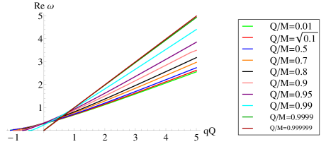
Figure 1: Dependence of Re $\omega$ on the charge $qQ$ of the scalar field with the mass $\mu=0.05$ and the orbital momentum $l=1$. Different extremalities are shown in different colors.

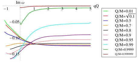
Figure 2: Dependence of Im $\omega$ on the charge $qQ$ of the scalar field with the mass $\mu=0.05$ and the orbital momentum $l=1$. Different extremalities are shown in different colors.

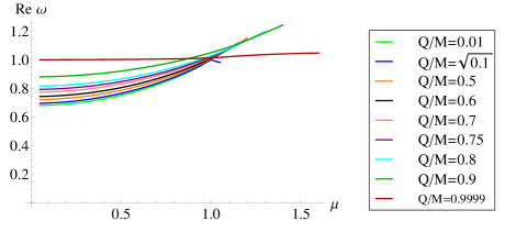
Figure 3: Dependence of Re $\omega$ on the mass $\mu$ of the scalar field with the charge $qQ=1$ and the orbital momentum $l=1$.

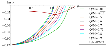
Figure 4: Dependence of Im $\omega$ on the mass $\mu$ of the scalar field with the charge $qQ=1$ and the orbital momentum $l=1$.

As the effects of noncommutative deformation in our model are not clearly visible from Figures 1-4, we have introduced a quantity called frequency splitting, which is defined as $\omega^{\pm}=\omega_{m=\pm 1}-\omega_{m=0},$ where $m=-l,\ -l+1,...,l$ is the projection of the orbital angular momentum $l$. In case that the orbital angular momentum $l$ is greater than $1,$ the frequency splitting receives a generalization in the form $\omega^{\pm\pm\cdot\cdot\cdot\pm}=\omega_{m}-\omega_{m=0}$. Specifically, $\omega^{\pm\pm}=\omega_{m=\pm 2}-\omega_{m=0}$. Here we shall consider only quantities $\omega^{\pm}$ and $\omega^{\pm\pm}$. They are demonstrated at Figures 5 and 6 for the angular momentum channel $l=2$ and for the value of the ratio $\frac{Q}{M}=0.5$. On these figures the real and the imaginary part of the frequency splittings $\omega^{\pm}$ and $\omega^{\pm\pm}$ is shown as a function of the scalar field charge $q$. The frequency splitting can be graphically presented for any value of the ratio $\frac{Q}{M}$.

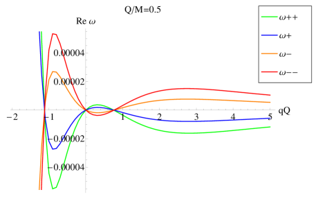
Figure 5: Dependence of Re $\omega^{\pm}$, Re $\omega^{\pm\pm}$ on the charge $qQ$ of the scalar field with the mass $\mu=0.05$, orbital momentum $l=2$ and extremality $\frac{Q}{M}=0.5$.

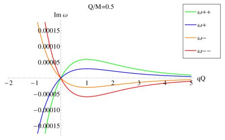
Figure 6: Dependence of Im $\omega^{\pm}$, Im $\omega^{\pm\pm}$ on the charge $qQ$ of the scalar field with the mass $\mu=0.05$, orbital momentum $l=2$ and extremality $\frac{Q}{M}=0.5$.

3.2 Analytic method in the near extremal approximation

The second approach that we adopt here is based on an analytic method [72],[73] which is however only accurate in a highly restrictive regime of system parameters that is related to conditions of near extremality. The main idea behind this approach is to solve separately the equation (2.16) in two distinct regions, first in the region relatively close to the horizon and then in the region relatively far from the horizon and afterwards to extrapolate both solutions into a region of common overlap. As a result of matching of the two extrapolated solutions, the quantization condition emerges that determines a QNM spectrum for the scalar perturbations of the RN black hole. This quantization condition is given by

$$\begin{split}&\frac{\Gamma(1-2i\sigma)\Gamma(-2i\sigma-2\tilde{\rho})}{\Gamma(\frac{1}{2}-i\sigma-ik-\tilde{\rho})\Gamma(\frac{1}{2}-i\sigma+ik-i\Omega-\tilde{\rho})\Gamma(\frac{1}{2}-i\sigma-i\kappa)}\\ &=-\frac{\Gamma(1+2i\sigma)\Gamma(2i\sigma+2\tilde{\rho})\tau^{-2\tilde{\rho}}}{\Gamma(\frac{1}{2}+i\sigma-ik+\tilde{\rho})\Gamma(\frac{1}{2}+i\sigma+ik-i\Omega+\tilde{\rho})\Gamma(\frac{1}{2}+i\sigma-i\kappa)}\\ &\times{\Big{(}-2i\sqrt{\omega^{2}-\mu^{2}}~{}r_{+}\tau\Big{)}}^{-2i\sigma},\end{split}$$ (3.23)

where the quantities $\tilde{\rho},k,\sigma,,\kappa,\Omega$ are all functions of the system parameters (the mass and the charge of the RN black hole, as well as the mass and the charge of the scalar field), the frequency $\omega$ and the deformation parameter $a$. In addition, $\tau$ is the extremality parameter, $\tau=\frac{r_{+}-r_{-}}{r_{+}}.$ For details see the reference [28]. In general, this condition cannot be solved analytically. In the following, we present some numerical results for the QNM frequencies, obtained by Wolfram Mathematica which result from the analytic condition (3.23). In particular, only the fundamental quasinormal mode will be analysed.

In this way Figures 7 and 8 show a dependence of the real and imaginary part of the fundamental QNM frequency $\omega$ on the charge $q$ of the scalar field. In order to make comparison for different (albeit still close to $1$) values of the ratio $\frac{Q}{M}$, we plot the results for two choices of ”extremality”: $\frac{Q}{M}=0.9999$ and $\frac{Q}{M}=0.999999$. The former one corresponds to the ”extremality” parameter $\tau=0.0278891617$, while the latter corresponds to $\tau=0.0028244321$. It is important to note that a derivation of the condition (3.23) was made within the approximation that the NC deformation parameter $a$ is of the same order as the extremality $\tau$. Therefore, in the case $\frac{Q}{M}=0.9999$ we set $a=0.1,$ while in the case $\frac{Q}{M}=0.999999$ we set $a=0.01$. The $q$ dependance of $\mbox{Re}\,\omega$ and $\mbox{Im}\,\omega$ is presented in Figures 7 and 8, where it was assumed that the mass of the scalar field is fixed at $\mu=0.05$.

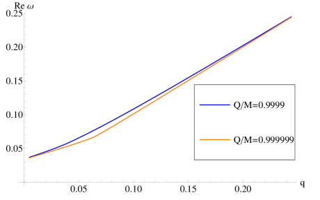
Figure 7: Dependance of $\mbox{Re}\,\omega$ on the charge $q$ of the scalar field with the mass $\mu=0.05$, $l=1$.

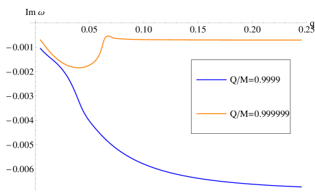
Figure 8: Dependance of $\mbox{Im}\,\omega$ on the charge $q$ of the scalar field with the mass $\mu=0.05$, $l=1$.

Likewise, the dependance of the fundamental QNM frequency $\omega$ on the mass $\mu$ of the scalar field, for the fixed charge $q=0.075$, is shown in Figures 9 and 10.

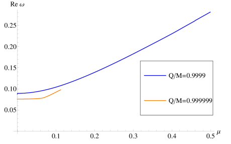
Figure 9: Dependance of $\mbox{Re}\,\omega$ on the mass $\mu$ of the scalar field with the charge $q=0.075$, $l=1$.

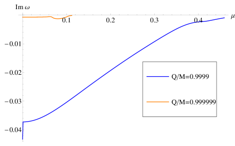
Figure 10: Dependance of $\mbox{Im}\,\omega$ on the mass $\mu$ of the scalar field with the charge $q=0.075$, $l=1$.

As in a previous method, a non-zero NC effect on the QNM spectrum may be inferred by studying the quantities called frequency splitting. They were already defined before and denoted as $\omega^{\pm}$, $\omega^{\pm\pm}$. Figures 11 and 12 show a dependance of the real and imaginary part of the frequency splittings $\omega^{\pm}$, $\omega^{\pm\pm}$ on the scalar field charge $q$. The graphs are made for the following set of parameters: $Q/M=0.999999$, $\mu=0.05$ and $l=2$.

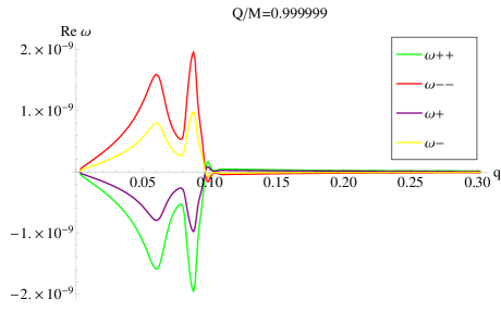
Figure 11: Dependance of frequency splitting of $\mbox{Re}\,\omega$ on the charge $q$ of the scalar field with the mass $\mu=0.05$, $l=2$.

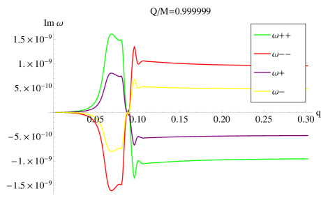
Figure 12: Dependance of frequency splitting of $\mbox{Im}\,\omega$ on the charge $q$ of the scalar field with the mass $\mu=0.05$, $l=2$.

Two latter figures clearly demonstrate a phenomenon of frequency splitting, indicating lines that correspond to $m=\pm 2$ and $m=\pm 1$. In this way they show the same patterns already outlined at Figures 5 and 6, thus supporting the findings obtained by the continued fraction method. This effect, though being very tiny, is qualitatively very important, as it indicates a presence of NC driven features in the QNM spectrum, thus signalling an essentially quantum nature of spacetime. Since the frequency splitting has its origin in a coupling between the deformation parameter $a$ and the azimuthal (magnetic) quantum number $m$ (see equation (2.16)), this effect is reminiscent of a Zeeman-like splitting in the spectrum of the hydrogen-like atoms, with deformation $a$ taking the role of a magnetic field.

Interestingly, all figures related to frequency splitting (Figures 5,6,11,12) show the same property, namely $~{}{\omega^{+}}=-{\omega^{-}}~{}$ and $~{}{\omega^{++}}=-{\omega^{--}}.~{}$ This feature was expected due to a parity symmetry of the model considered. Other features where two methods agree qualitatively in their findings include: the appearance of quasi-resonances in the spectrum, the existence of constant values at which the imaginary part of the QNM frequency saturates and the appearance of the linearly dependent pattern for larger values of $qQ$, representing the real part of the QNM frequency as a function of the charge $q$ .

Besides QNM spectra of black holes, there are many other important concepts in physics which may require an appropriate reassessment in terms of quantum nature of spacetime, such as the geodesic and quantum completeness [74], the existence of naked singularities and related issue of validness of the cosmic censorship hypothesis [75], the renormalization of black hole entanglement entropy [76] and a description of physics in terms of fuzzy (Anti)-de Sitter space [77],[78],[79],[80] to name a few. We think that these issues should be given a considerable attention in future studies.

Acknowledgement The work of M.D.C. and N.K. is supported by project ON171031 of the Serbian Ministry of Education and Science. The work of A.S. is partially supported by the project RBI-TWINN-SIN. This work is partially supported by ICTP-SEENET-MTP Project NT-03 ”Cosmology-Classical and Quantum Challenges” in frame of the Southeastern European Network in Theoretical and Mathematical Physics. A.S. would like to thank the organizers of the XXVIth International Conference on Integrable Systems and Quantum symmetries (ISQS-26) for their hospitality.

References

References

- [1] G. Amelino-Camelia and L. Smolin, Phys. Rev. D 80 (2009) 084017.
- [2] G. Amelino-Camelia, Living Rev. Rel. 16 (2013) 5.
- [3] T. Jacobson, S. Liberati and D. Mattingly, Annals Phys. 321 (2006) 150.
- [4] G. Amelino-Camelia, J. Ellis, N.E. Mavromatos, D.V. Nanopoulos and S. Sarkar, Nature 393 (1998) 763.
- [5] R. Gambini and J. Pullin, Phys. Rev. D 59 (1999) 124021.
- [6] B.E. Schaefer, Phys. Rev Lett. 82 (1999) 4964.
- [7] S.D. Biller et al, Phys. Rev. Lett. 83 (1999) 2108.
- [8] J. Alfaro, H.A. Morales-Tecotl and L.F. Urrutia, Phys. Rev. Lett. 84, 2318 (2000).
- [9] G. Amelino-Camelia, L. Barcaroli, G. D’Amico, N. Loret and G. Rosati, Phys. Lett. B 761 (2016) 318.
- [10] G. Amelino-Camelia, Int. J. Mod. Phys. D 11 (2002) 35.
- [11] G. Amelino-Camelia, Phys. Lett. B 510 (2001) 255.
- [12] J. Kowalski-Glikman, Phys. Lett. A 286 (2001) 391.
- [13] N.R. Bruno, G. Amelino-Camelia and J. Kowalski-Glikman, Phys. Lett. B 522 (2001) 133.
- [14] J. Magueijo and L. Smolin, Phys. Rev. Lett. 88 (2002) 190403.
- [15] G. Amelino-Camelia, L. Freidel, J. Kowalski-Glikman and L. Smolin, Phys. Rev. D 84 (2011) 084010.
- [16] G. Amelino-Camelia, N. Loret and G. Rosati, Phys. Lett. B 700 (2011) 150.
- [17] S. Meljanac, A. Pachol, A. Samsarov and K. S. Gupta, Phys. Rev. D 87 (2013) no.12, 125009.
- [18] S. Mignemi and A. Samsarov, Phys. Lett. A 381 (2017) 1655.
- [19] S. Mignemi and G. Rosati, Class. Quant. Grav. 35 (2018) no.14, 145006.
- [20] J. Kowalski-Glikman and S. Nowak, Phys. Lett. B 539 (2002) 126.
- [21] J. Kowalski-Glikman and S. Nowak, Int. J. Mod. Phys. D 12 (2003) 299.
- [22] A. Borowiec and A. Pachol, Phys. Rev. D 79 (2009) 045012
- [23] A. Borowiec and A. Pachol, SIGMA 6 (2010) 086.
- [24] T. Jurić, S. Meljanac, D. Pikutić and R. Štrajn, JHEP 1507 (2015) 055.
- [25] P. Aschieri, A. Borowiec and A. Pachol, JHEP 1710 (2017) 152.
- [26] A. Abdo et al., Science 323 (2009) 1688.
- [27] B. P. Abbott et al., Observation of Gravitational Waves from a Binary Black Hole Merger, Phys. Rev. Lett. 116 (2016) 061102.
- [28] M. D. Ćirić, N. Konjik and A. Samsarov, Class. Quant. Grav. 35 (2018) no.17, 175005.
- [29] M. D. Ćirić, N. Konjik and A. Samsarov, Noncommutative scalar field in the non-extremal Reissner-Nordström background: QNM spectrum, arXiv:1904.04053 [hep-th].
- [30] K. S. Gupta, E. Harikumar, T. Jurić, S. Meljanac and A. Samsarov, JHEP 1509 (2015) 025.
- [31] K. S. Gupta, T. Jurić and A. Samsarov, JHEP 1706 (2017) 107.
- [32] T. Regge and J. A. Wheeler, Stability of a Schwarzschild singularity, Phys. Rev. 108, 1063 (1957).
- [33] C.V. Vishveshwara, Scattering of Gravitational Radiation by a Schwarzschild Black-hole, Nature 227, 936 (1970).
- [34] W. H. Press, Long Wave Trains of Gravitational Waves from a Vibrating Black Hole, Astrophys. J. 170, L105 (1971).
- [35] S. Chandrasekhar and S. L. Detweiler, The quasi-normal modes of the Schwarzschild black hole, Proc. R. Soc. A 344, 441 (1975).
- [36] V. Ferrari and B. Mashhoon, New approach to the quasinormal modes of a black hole, Phys. Rev. D 30, 295 (1984).
- [37] H. P. Nollert, Quasinormal modes: the characteristic ”sound” of black holes and neutron stars, Class. Quant. Grav. 16 (1999), R159.
- [38] K. D. Kokkotas and B. G. Schmidt, Quasinormal modes of stars and black holes, Living Rev. Rel. 2 (1999) 2.
- [39] E. Berti, V. Cardoso and A. O. Starinets, Quasinormal modes of black holes and black branes, Class. Quant. Grav. 26, 163001 (2009).
- [40] R. A. Konoplya and A. Zhidenko, Quasinormal modes of black holes: From astrophysics to string theory, Rev. Mod. Phys. 83, 793 (2011).
- [41] V. Cardoso and J. P. S. Lemos, Scalar, electromagnetic and Weyl perturbations of BTZ black holes: Quasinormal modes, Phys. Rev. D 63 (2001) 124015.
- [42] V. Cardoso and J. P. S. Lemos, Quasinormal modes of Schwarzschild anti-de Sitter black holes: Electromagnetic and gravitational perturbations, Phys. Rev. D 64 (2001) 084017.
- [43] W. Israel, Phys. Rev. 164, 1776 (1967); Commun. Math. Phys. 8, 245 (1968).
- [44] B. Carter, Phys. Rev. Lett. 26, 331 (1971).
- [45] S. W. Hawking, Commun. Math. Phys. 25, 152 (1972).
- [46] D. C. Robinson, Phys. Rev. D 10, 458 (1974); Phys. Rev. Lett. 34, 905 (1975).
- [47] J. Isper, Phys. Rev. Lett. 27, 529 (1971).
- [48] A. E. Mayo and J. D. Bekenstein, Phys. Rev. D 54, 5059 (1996).
- [49] A. Connes, Non-commutative Geometry, Academic Press (1994).
- [50] G. Landi, An introduction to noncommutative spaces and their geometry, Springer, New York (1997); arXiv:hep-th/9701078.
- [51] J. Madore, An Introduction to Noncommutative Differential Geometry and its Physical Applications, 2nd Edition, Cambridge Univ. Press (1999).
- [52] P. Aschieri, M. Dimitrijević, P. Kulish, F. Lizzi and J. Wess Noncommutative spacetimes: Symmetries in noncommutative geometry and field theory, Lecture notes in physics 774, Springer (2009).
- [53] M. Daszkiewicz, J. Lukierski and M. Woronowicz, Mod. Phys. Lett. A 23 (2008) 653.
- [54] M. Daszkiewicz, J. Lukierski and M. Woronowicz, Phys. Rev. D 77 (2008) 105007.
- [55] C. A. S. Young and R. Zegers, Nucl. Phys. B 797 (2008) 537
- [56] C. A. S. Young and R. Zegers, Nucl. Phys. B 809 (2009) 439.
- [57] T. R. Govindarajan, K. S. Gupta, E. Harikumar, S. Meljanac and D. Meljanac, Phys. Rev. D 80 (2009) 025014.
- [58] S. Meljanac, D. Meljanac, A. Samsarov and M. Stojic, Phys. Rev. D 83 (2011) 065009.
- [59] S. Meljanac, A. Samsarov and R. Strajn, JHEP 1208 (2012) 127.
- [60] B. Ivetic, S. Mignemi and A. Samsarov, Phys. Rev. D 94 (2016) no.6, 064064.
- [61] M. Dimitrijević Ćirić, N. Konjik, M. A. Kurkov, F. Lizzi, P. Vitale, Noncommutative field theory from angular twist, Phys. Rev. D 98 (2018), 085011.
- [62] M. Dimitrijević Ćirić, B. Nikolić and V. Radovanović, Noncommutative gravity and the relevance of the theta-constant deformation, EPL 118, 2 (2017).
- [63] P. Aschieri and L. Castellani, Noncommutative gravity coupled to fermions JHEP, 0906, 086 (2009).
- [64] P. Aschieri and L. Castellani, Noncommutative gravity coupled to fermions: second order expansion via Seiberg-Witten map, JHEP 1207 184 (2012).
- [65] M. Richartz, Phys. Rev. D 93 (2016) no.6, 064062.
- [66] W. Gautschi, Computational Aspects of Three-Term Recurrence Relations, SIAM Rev. 9 (1967) 24.
- [67] E. W. Leaver, An Analytic representation for the quasi normal modes of Kerr black holes, Proc. R. Soc. A 402, (1985) 285.
- [68] H. P. Nollert, Quasinormal modes of Schwarzschild black holes: The determination of quasinormal frequencies with very large imaginary parts, Phys. Rev. D 47, (1993) 5253.
- [69] R. A. Konoplya and A. Zhidenko, Massive charged scalar field in the Kerr-Newman background I: quasinormal modes, late-time tails and stability, Phys. Rev. D 88 (2013) 024054.
- [70] M. Richartz and D. Giugno, Quasinormal modes of charged fields around a Reissner-Nordström black hole, Phys. Rev. D 90, (2014) 124011.
- [71] A. Chowdhury and N. Banerjee, Quasinormal modes of a charged spherical black hole with scalar hair for scalar and Dirac perturbations, Eur. Phys. J. C 78, (2018) 594.
- [72] S. Hod, Relaxation dynamics of charged gravitational collapse, Phys. Lett. A 374, (2010) 2901.
- [73] S. Hod, Eur. Phys. J. C 77 (2017) no.5, 351.
- [74] T. Jurić, JHEP 1805 (2018) 007.
- [75] K. S. Gupta, T. Jurić, A. Samsarov and I. Smolić, arXiv:1908.07402 [hep-th].
- [76] T. Jurić and A. Samsarov, Phys. Rev. D 93 (2016) no.10, 104033.
- [77] M. Buric and J. Madore, “Noncommutative de Sitter and FRW spaces”, Eur. Phys. J. C. 10 (2015) 75.
- [78] M. Buric and D. Latas, Discrete fuzzy de Sitter cosmology, Phys. Rev. D 100 (2019) 024053.
- [79] D. Jurman and H. Steinacker, JHEP 1401 (2014) 100.
- [80] D. Jurman, Fortsch. Phys. 67 (2019) no.4, 1800061.