On Generalization Bounds of a Family of Recurrent Neural Networks

Abstract

Recurrent Neural Networks (RNNs) have been widely applied to sequential data analysis. Due to their complicated modeling structures, however, the theory behind is still largely missing. To connect theory and practice, we study the generalization properties of vanilla RNNs as well as their variants, including Minimal Gated Unit (MGU), Long Short Term Memory (LSTM), and Convolutional (Conv) RNNs. Specifically, our theory is established under the PAC-Learning framework. The generalization bound is presented in terms of the spectral norms of the weight matrices and the total number of parameters. We also establish refined generalization bounds with additional norm assumptions, and draw a comparison among these bounds. We remark: (1) Our generalization bound for vanilla RNNs is significantly tighter than the best of existing results; (2) We are not aware of any other generalization bounds for MGU, LSTM, and Conv RNNs in the exiting literature; (3) We demonstrate the advantages of these variants in generalization.

1 Introduction

Recurrent Neural Networks (RNNs) have successfully revolutionized sequential data analysis, and been widely applied to many real world problems, such as natural language processing (Cho et al., 2014; Bahdanau et al., 2014; Sutskever et al., 2014), speech recognition (Graves et al., 2006; Mikolov et al., 2010; Graves, 2012; Graves et al., 2013), computer vision (Gregor et al., 2015; Xu et al., 2015; Donahue et al., 2015; Karpathy and Fei-Fei, 2015), healthcare (Lipton et al., 2015; Choi et al., 2016a, b), and robot control (Lee and Teng, 2000; Yoo et al., 2006). Quite a few of these applications can be approached easily in our daily life, such as Google Translate, Google Now, Apple Siri, etc.

The sequential modeling nature of RNNs is significantly different from feedforward neural networks, though they both have neurons as the basic components. RNNs exploit the internal state (also known as hidden unit) to process the sequence of inputs, which naturally captures the dependence of the sequence. Besides the vanilla version, RNNs have many other variants. A large class of variants incorporate the so-called “gated” units to trim RNNs for different tasks. Typical examples include Long Short-Term Memory (LSTM, Hochreiter and Schmidhuber (1997)), Gated Recurrent Unit (GRU, Jozefowicz et al. (2015)) and Minimal Gated Unit (MGU, Zhou et al. (2016)).

The success of RNNs owes not only to their special network structures and the ability to fit data, but also to their good generalization property: They provide accurate predictions on unseen data. For example, Graves et al. (2013) report that after training with merely 462 speech samples, deep LSTM RNNs achieve a test set error of $17.7\%$ on TIMIT phoneme recognition benchmark, which is the best recorded score. Despite of the popularity of RNNs in applications, their theory is less studied than other feedforward neural networks (Haussler, 1992; Bartlett et al., 2017; Neyshabur et al., 2017; Golowich et al., 2017; Li et al., 2018). There are still several long lasting fundamental questions regarding the approximation, trainability, and generalization of RNNs.

In this paper, we propose to understand the generalization ability of RNNs and their variants. We aim to answer two questions from a theoretical perspective:

Q.1) Do RNNs suffer from significant curse of dimensionality?

Q.2) What are the advantages of MGU and LSTM over vanilla RNNs?

The investigation of generalization properties of RNNs has a long history. Many early works are based on oversimplified assumptions. Dasgupta and Sontag (1996) and Koiran (1998), for example, adopt a VC-dimension argument to show complexity bounds of RNNs that are polynomial in the size of the network. They, however, either consider linear RNNs for binary classification tasks, or assume RNNs take the first coordinate of their hidden states as outputs. More recently, Bartlett et al. (2017) propose a new technique for developing generalization bounds for feedforward neural networks based on empirical Rademacher complexity under the PAC-Learning framework. Neyshabur et al. (2017) further adapt the technique to establish their generalization bound using the PAC-Bayes approach. The follow-up work Zhang et al. (2018) use the PAC-Bayes approach to establish a generalization bound for vanilla RNNs.

We exploit the compositional nature of RNNs, and decouples the spectral norms of weight matrices and the number of weight parameters. This makes our analysis conceptually much simpler (e.g. avoid layer wise analysis), and also yields better generalization bound than Zhang et al. (2018).

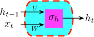
Figure 1: A building block of vanilla RNNs.

Consider vanilla RNNs, we observe $m$ sequences of data points $\left(x_{i,t},z_{i,t}\right)_{t=1}^{T}$, where $x_{i,t}\in\mathbb{R}^{d_{x}}$ and the response $z_{i,t}\in\mathcal{Z}$ for all $t=1,...,T$ and $i=1,...,m$. Each sequence is drawn independently from some underlying distribution over $\mathbb{R}^{d_{x}\times T}\times\mathcal{Z}$. Extensions to dependent sequences are discussed in Section 7, however, note that data points $(x_{i,t},z_{i,t})$ can be dependent within a sequence, i.e., for a fixed $i\in\{1,\dots,m\}$. The vanilla RNNs compute $h_{i,t}$ and $y_{i,t}$ iteratively as follows,

$$h_{i,t}=\sigma_{h}\left(Uh_{i,t-1}+Wx_{i,t}\right),\quad\textrm{and}\quad y_{i,t}=\sigma_{y}\left(Vh_{i,t}\right),$$

where $\sigma_{y}$ and $\sigma_{h}$ are activation operators, $h_{i,t}\in\mathbb{R}^{d_{h}}$ is the hidden state with $h_{i,0}=0$, and $U\in\mathbb{R}^{d_{h}\times d_{h}}$, $V\in\mathbb{R}^{d_{y}\times d_{h}}$, and $W\in\mathbb{R}^{d_{h}\times d_{x}}$ are weight matrices. The activation operators $\sigma_{h}$ and $\sigma_{y}$ are entrywise, i.e., $\sigma_{h}(\left[v_{1},\dots,v_{d}\right]^{\top})=[\sigma_{h}(v_{1}),\dots,\sigma_{h}(v_{d})]^{\top}$, and Lipschitz with parameters $\rho_{h}$ and $\rho_{y}$ respectively. We assume $\sigma_{h}(\cdot)=\tanh(\cdot)$, $\sigma_{y}(0)=0$, and $\rho_{y}=1$. Extensions to general activations are given in Section 2.

Our Contribution. To establish the generalization bound, we need to define the “model complexity” of vanilla RNNs. In this paper, we adopt the empirical Rademacher complexity (ERC, see more details in Section 2), which has been widely used in the existing literature on PAC-Learning. For many nonparametric function classes, we often need complicated argument to upper bound their ERC. Our analysis, however, shows that we can upper bound the ERC of vanilla RNNs in a very simple manner by exploiting their Lipschitz continuity with respect to the model parameters, since they are essentially in parametric forms. More specifically, denote $\mathcal{F}_{t}=\{f_{t}:\{x_{1},...,x_{t}\}\mapsto y_{t}\}$ as the class of mappings from the first $t$ inputs to the $t$-th output computed by vanilla RNNs. For a matrix $A$, $\lVert A\rVert_{2}$ denotes the spectral norm, and for a vector $v$, $\lVert v\rVert_{2}$ denotes the Euclidean norm. Define $\frac{a^{t}-1}{a-1}=t$ for $a=1$. Then, informally speaking, the “model complexity” of vanilla RNNs satisfies

$$\textsf{Complexity}=O\Bigg{(}d\lVert V\rVert_{2}\min\big{\{}\sqrt{d},\lVert W\rVert_{2}\frac{\lVert U\rVert_{2}^{t}-1}{\lVert U\rVert_{2}-1}\big{\}}\times\sqrt{\log\left(t\sqrt{d}\frac{\lVert U\rVert_{2}^{t}-1}{\lVert U\rVert_{2}-1}\right)}\Bigg{)},$$

where $d=\sqrt{d_{x}d_{h}+d_{h}^{2}+d_{h}d_{y}}$.

We then consider a new testing sequence $\left(x_{t},z_{t}\right)_{t=1}^{T}$. The response sequence is computed by $\widetilde{z}_{t}=\phi(y_{t}),\quad\text{for all}~{}t=1,\dots,T,$ where $\phi$ is a function mapping the output of vanilla RNNs to the response of interest. In practice, the function $\phi$ varies across different data analysis tasks. For example, in sequence to sequence classification, we take $\phi(y_{t})=\mathop{\mathrm{argmax}}_{j}[y_{t}]_{j}$; in regression, we take $\phi(y_{t})=y_{t}$; in density estimation, we can take $\phi(y_{t})=\textrm{softmax}(y_{t})$.

We further define a risk function that can unify different data analysis tasks. Specifically, let $\mathcal{L}(\mathcal{A}(y,z))$ be a loss function, where $\mathcal{A}(y,z)$ is a function taking the output $y_{t}$ and the observed response $z_{t}$ as inputs, and $\mathcal{L}$ is chosen according to different tasks. Then we define the population risk for the $t$-th output as $\mathcal{R}(f_{t})=\mathbb{E}[\mathcal{L}(\mathcal{A}(y_{t},z_{t}))]$. Its empirical counterpart is similarly defined as $\widehat{\mathcal{R}}(f_{t})=\frac{1}{m}\sum_{i=1}^{m}\mathcal{L}(\mathcal{A}(y_{i,t},z_{i,t}))$. Training RNNs is essentially minimizing the empirical risk $\widehat{\mathcal{R}}(f_{t})$. Many applications can be formulated into this framework. For example, in classification, we take $\mathcal{A}=-\mathcal{M}$ as the functional margin operator and $\mathcal{L}=\mathcal{L}_{\gamma}$ as the ramp loss with $\gamma$ being the margin value (see detailed definitions in Section 2); in regression, we take $\mathcal{A}(y_{t},z_{t})=y_{t}-z_{t}$ and $\mathcal{L}$ as the $\ell_{p}$ loss for $p\in\mathbb{Z}_{+}$. We then give the generalization bound in the following statement.

Theorem 1 (informal).

Assume the input data space is bounded, i.e., $\|x\|_{2}\leq 1$ and $z\in\mathcal{Z}$ bounded. Suppose the mapping $\mathcal{A}(y,z)$ is Lipschitz in $y$, and the loss function $\mathcal{L}$ satisfies $|\mathcal{L}(\mathcal{A}(y,z))|\leq B$ and is $L$-Lipschitz for any $y$ computed by RNNs and $z\in\mathcal{Z}$. Given a collection of samples $S=\left\{(x_{i,t},z_{i,t})_{t=1}^{T},i=1,...,m\right\}$ and a new testing sequence $(x_{t},z_{t})_{t=1}^{T}$, with probability at least $1-\delta$ over $S$, for any $f_{t}\in\mathcal{F}_{t}$ with integer $t\leq T$, we have,

$$\mathcal{R}(f_{t})\leq\widehat{\mathcal{R}}(f_{t})+\widetilde{O}\bigg{(}\frac{L\times\textsf{Complexity}}{\sqrt{m}}+B\sqrt{\frac{\log(1/\delta)}{m}}\bigg{)}.$$

Please refer to Section 2 for a complete statement. Most of the aforementioned commonly used $\mathcal{A}$ and $\mathcal{L}$ satisfy the assumptions in Theorem 1. For example, in classification, the functional margin operator $\mathcal{M}(y,z)$ is $2$-Lipschitz in $\widetilde{z}$. The ramp loss $\mathcal{L}_{\gamma}$ is uniformly bounded by $1$ and $\frac{1}{\gamma}$-Lipschitz. In regression, $\mathcal{A}(y,z)$ is $1$-Lipschitz in $y$ and bounded since the input data are bounded. Then the $\ell_{p}$ loss becomes bounded and Lipschitz due to its bounded input.

Comparison with Existing Results. To better understand the obtained generalization bound and draw a comparison among existing literature, we instantiate Theorem 1 for sequence to sequence classification using vanilla RNNs. Recall that for classification tasks, we have $L=1/\gamma$, $B=1$ and $\mathcal{M}(y,z)$ is $2$-Lipschitz in $y$. We list the corresponding generalization bounds in Table 1 according to the magnitude of $\|U\|_{2}$.

Table 1: Generalization bounds for vanilla RNNs in classification tasks (we only list the order of the gap $\mathcal{R}(f_{t})-\widehat{\mathcal{R}}(f_{t})$). The third column lists the result obtained in Zhang et al. (2018).

	Theorem 1	Zhang et al. (2018)
(I) $\|U\|_{2}<1$	$\widetilde{O}\big{(}d/\sqrt{m}\gamma\big{)}$	$\widetilde{O}\big{(}dt^{2}/\sqrt{m}\gamma\big{)}$
(II) $\lVert U\rVert_{2}=1$	$\widetilde{O}\big{(}dt/\sqrt{m}\gamma\big{)}$	$\widetilde{O}\big{(}dt^{2}/\sqrt{m}\gamma\big{)}$
(III) $\lVert U\rVert_{2}>1$	$\widetilde{O}\big{(}\sqrt{d^{3}t}/\sqrt{m}\gamma\big{)}$	$\widetilde{O}\big{(}dt^{2}\lVert U\rVert_{2}^{t}/\sqrt{m}\gamma\big{)}$

As can be seen, the obtained generalization bound only has a polynomial dependence on the size of vanilla RNNs, i.e., width $d$ and sequence length $t$. Thus, we theoretically justify that the complexity of vanilla RNNs do not suffer from significant curse of dimensionality. Because they compute outputs $y_{t}$ recursively using the same weight matrices, and their hidden states $h_{t}$ are entrywise bounded.

We compare Theorem 1 with the generalization bound obtained in Zhang et al. (2018), which is of the order $\widetilde{O}\left(dt^{2}\lVert W\rVert_{2}\lVert V\rVert_{2}\max\{1,\lVert U\rVert_{2}^{t}\}/\sqrt{m}\gamma\right),$ and we distinguish the same three different scenarios as listed in Table 1. Our bound is tighter by a factor of $t^{2}$ for case (I), a factor of $t$ for case (II). Additionally, Zhang et al. (2018) fail to incorporate the boundedness condition of hidden state into their analysis, thus the generalization bound is exponential in $t$ for case (III). Our generalization bound, however, is still polynomial in $d$ and $t$ for case (III).

Moreover, (II) is closely related to a few recent results on imposing orthogonal constraints on weight matrices to stabilize the training of RNNs (Saxe et al., 2013; Le et al., 2015; Arjovsky et al., 2016; Vorontsov et al., 2017; Zhang et al., 2018). We remark that from a learning theory perspective, (II) implies that orthogonal constraints can potentially help generalization.

We also present refined generalization bounds with additional matrix norm assumptions. These assumptions allow us to derive norm-based generalization bounds. We draw a comparison among these bounds and highlight their advantage under different scenarios.

Our theory can be further extended to several variants, including MGU and LSTM RNNs, and convolutional RNNs (Conv RNNs). Specifically, we show that the gated units in MGU and LSTM RNNs can introduce extra decaying factors to further reduce the dependence on $d$ and $t$ in generalization. The convolutional filters in Conv RNNs can reduce the dependence on $d$ through parameter sharing. Such an advantage in generalization makes these RNNs do not suffer from significant curse of dimensionality. To the best of our knowledge, these are the first results on generalization guarantees for these neural networks.

Notations: Given a vector $v\in\mathbb{R}^{d}$, we denote its Euclidean norm by $\lVert v\rVert_{2}^{2}=\sum_{i=1}^{d}|v_{i}|^{2}$, and the infinity norm by $\lVert v\rVert_{\infty}=\max_{j}|v_{j}|$. Given a matrix $M\in\mathbb{R}^{m\times n}$, we denote the spectral norm by $\lVert M\rVert_{2}$ as the largest singular value of $M$, the Frobenius norm by $\lVert M\rVert_{\textrm{F}}^{2}=\textrm{trace}(MM^{\top})$, and the $(2,1)$ norm by $\|M\|_{2,1}=\sum_{i=1}^{n}\|M_{:,i}\|_{2}$. Given a function $f$, we denote the function infinity norm by $\lVert f\rVert_{\infty}=\sup|f|$. We use $\widetilde{O}(\cdot)$ to denote $O(\cdot)$ with hidden log factors.

2 Generalization of Vanilla RNNs

To establish the generalization bound, we start with imposing some mild assumptions.

Assumption 1.

Input data are bounded, i.e., $\lVert x_{i,t}\rVert_{2}\leq B_{x}$ for all $i=1,\dots,m$ and $t=1,\dots,T$.

Assumption 2.

The spectral norms of weight matrices are bounded respectively, i.e., $\lVert U\rVert_{2}\leq B_{U}$, $\lVert V\rVert_{2}\leq B_{V},$ and $\lVert W\rVert_{2}\leq B_{W}.$

Assumption 3.

Activation operators $\sigma_{h}$ and $\sigma_{y}$ are Lipschitz with parameters $\rho_{h}$ and $\rho_{y}$ respectively, and $\sigma_{h}(0)=\sigma_{y}(0)=0$. Additionally, $\sigma_{h}$ is entrywise bounded by $b$.

Assumptions 1 and 2 are moderate assumptions. Moreover, Assumption 3 holds for most commonly used activation operators, such as $\sigma_{h}(\cdot)=\tanh(\cdot)$ and $\sigma_{y}(\cdot)=\textrm{ReLU}(\cdot)=\max\{\cdot,0\}$ (1-Lipschitz).

Recall vanilla RNNs compute $h_{i,t}$ and $y_{i,t}$ as follows,

$$h_{i,t}=\sigma_{h}\left(Uh_{i,t-1}+Wx_{i,t}\right)\quad\textrm{and}\quad y_{i,t}=\sigma_{y}\left(Vh_{i,t}\right),$$

where $U\in\mathbb{R}^{d_{h}\times d_{h}}$, $V\in\mathbb{R}^{d_{y}\times d_{h}}$, and $W\in\mathbb{R}^{d_{h}\times d_{x}}$. We consider multiclass classification tasks with the label $z\in\mathcal{Z}=\{1,\dots,K\}$. Given a sequence $(x_{t},z_{t})_{t=1}^{T}$, we define $X_{t}\in\mathbb{R}^{d_{x}\times t}$ by concatenating $x_{1},\dots,x_{t}$ as columns of $X_{t}$. Recall that we denote $\mathcal{F}_{t}=\{f_{t}:X_{t}\mapsto y_{t}\}$ as the class of mappings from the first $t$ inputs to the $t$-th output computed by vanilla RNNs.

As previously mentioned, we define the functional margin for the $t$-th output in vanilla RNNs as

$$\textstyle\mathcal{M}(f_{t}(X_{t}),z_{t})=[f_{t}(X_{t})]_{z_{t}}-\max_{j\neq z_{t}}[f_{t}(X_{t})]_{j}.$$

We further define a ramp loss $\mathcal{L}_{\gamma}\left(-\mathcal{M}(f_{t}(X_{t}),z_{t})\right):\mathbb{R}\mapsto\mathbb{R}^{+}$ to each margin, where $\mathcal{L}_{\gamma}$ is a piecewise linear function defined as

$$\mathcal{L}_{\gamma}(a)=\mathds{1}\{a>0\}+(1+a/\gamma)\mathds{1}\{-\gamma\leq a\leq 0\},$$

where $\mathds{1}\{A\}$ denotes the indicator function of a set $A$. Accordingly, the ramp risk is defined as

$$\mathcal{R}_{\gamma}(f_{t})=\mathbb{E}\left[\mathcal{L}_{\gamma}\left(-\mathcal{M}(f_{t}(X_{t}),z_{t})\right)\right],$$

and its empirical counterpart is defined as

$$\widehat{\mathcal{R}}_{\gamma}(f_{t})=\frac{1}{m}\sum_{i=1}^{m}\mathcal{L}_{\gamma}\left(-\mathcal{M}(f_{t}(X_{i,t}),z_{i,t})\right).$$

We then present the formal statement of Theorem 1.

Theorem 2.

Let activation operators $\sigma_{h}$ and $\sigma_{y}$ be given, and Assumptions 1–3 hold. Then for $(x_{t},z_{t})_{t=1}^{T}$ and $S=\left\{(x_{i,t},z_{i,t})_{t=1}^{T},i=1,\dots,m\right\}$ drawn i.i.d. from any underlying distribution over $\mathbb{R}^{d_{x}\times T}\times\{1,\dots,K\}$, with probability at least $1-\delta$ over $S$, for every margin value $\gamma>0$, sufficiently large sample size $m$, and every $f_{t}\in\mathcal{F}_{t}$ for integer $t\leq T$, we have

$$\mathbb{P}\left(\widetilde{z}_{t}\neq z_{t}\right)\leq\widehat{\mathcal{R}}_{\gamma}(f_{t})+3\sqrt{\frac{\log\frac{2}{\delta}}{2m}}+O\left(\frac{d\rho_{y}B_{V}\lambda_{t}\sqrt{\log\big{(}t\sqrt{dm}\frac{\beta^{t}-1}{\beta-1}\big{)}}}{\sqrt{m}\gamma}\right),$$ (1)

where $d=\sqrt{d_{x}d_{h}+d_{h}^{2}+d_{h}d_{y}}$, $\beta=\rho_{h}B_{U}$, and $\lambda_{t}=\min\big{\{}b\sqrt{d},\rho_{h}B_{x}B_{W}\frac{\beta^{t}-1}{\beta-1}\big{\}}$.

Remark 1.

To ease the presentation, we only provide the generalization bound for the classification task. Extensions to general tasks are straightforward by replacing functions $\mathcal{A}$ and $\mathcal{L}$ and substituting suitable values of $L$ and $B$.

The generalization bound depends on the total number of weights, and the range of $\rho_{h}B_{U}$ in three cases as indicated in Section 1. More precisely, if $\rho_{h}B_{U}\lesssim(1+\frac{1}{t^{\alpha}})$ for constant $\alpha>0$ bounded away from zero, the generalization bound is of the order $\widetilde{O}\left(\frac{dt^{\alpha}}{\sqrt{m}\gamma}\right)$, which has a polynomial dependence on $d$ and $t$. As can be seen, with proper normalization on model parameters, the model complexity of vanilla RNNs do not suffer from significant curse of dimensionality.

We also highlight a tradeoff between generalization and representation of vanilla RNNs. As can be seen, when $\rho_{h}B_{U}$ is strictly smaller than $1$, the generalization bound is nearly independent on $t$. The hidden state, however, only has limited representation ability, since its magnitude diminishes as $t$ grows large. On the contrary, when $\rho_{h}B_{U}$ is strictly greater than $1$, the representation ability is amplified but the generalization becomes worse. As a consequence, recent empirical results show that imposing extra constraints or regularization, such as $U^{\top}U=I$ or $\lVert U\rVert_{2}\leq 1$ (Saxe et al., 2013; Le et al., 2015; Arjovsky et al., 2016; Vorontsov et al., 2017; Zhang et al., 2018), helps balance the generalization and representation of RNNs.

3 Proof of Main Results

Our analysis is based on the PAC-learning framework. Due to space limit, we only present an outline of our proof. More technical details are deferred to Appendix A. Before we proceed, we first define the empirical Rademacher complexity as follows.

Definition 1 (Empirical Rademacher Complexity).

Let $\mathcal{H}$ be a function class and $S=\{s_{1},\dots,s_{m}\}$ be a collection of samples. The empirical Rademacher complexity of $\mathcal{H}$ given $S$ is defined as

$$\mathfrak{R}_{S}(\mathcal{H})=\mathbb{E}_{\epsilon}\left[\sup_{h\in\mathcal{H}}\frac{1}{m}\sum_{i=1}^{m}\epsilon_{i}h(s_{i})\right],$$

where $\epsilon_{i}$’s are i.i.d. Rademacher random variables, i.e., $\mathbb{P}(\epsilon_{i}=1)=\mathbb{P}(\epsilon_{i}=-1)=0.5$.

We then proceed with our analysis. Recall that Mohri et al. (2012) give an empirical Rademacher complexity (ERC)-based generalization bound, which is restated in the following lemma with $\mathcal{F}_{\gamma,t}=\left\{(X_{t},z_{t})\mapsto\ell_{\gamma}(-\mathcal{M}(f_{t}(X_{t}),z_{t})):f_{t}\in\mathcal{F}_{t}\right\}.$

Lemma 1.

Given a testing sequence $(x_{t},z_{t})_{t=1}^{T}$, with probability at least $1-\delta$ over samples $S=\left\{(x_{i,t},z_{i,t})_{t=1}^{T},i=1,\dots,m\right\}$, for every margin value $\gamma>0$ and any $f_{t}\in\mathcal{F}_{t}$, we have

$$\mathbb{P}(\widetilde{z}_{t}\neq z_{t})\leq\mathcal{R}_{\gamma}(f_{t})\leq\widehat{\mathcal{R}}_{\gamma}(f_{t})+2\mathfrak{R}_{S}(\mathcal{F}_{\gamma,t})+3\sqrt{\frac{\log(2/\delta)}{2m}}.$$

Note that Lemma 1 adapts the original version (Theorem 3.1, Chapter 3.1, Mohri et al. (2012)) for the multiclass ramp loss, and we have $\mathbb{P}(\widetilde{z}_{t}\neq z_{t})\leq\mathcal{R}_{\gamma}(f_{t})$ by definition.

Now we only need to bound the ERC $\mathfrak{R}_{S}(\mathcal{F}_{\gamma,t})$. Our analysis consists of three steps. First, we characterize the Lipschitz continuity of vanilla RNNs w.r.t model parameters. Next, we bound the covering number of function class $\mathcal{F}_{t}$. At last, we derive an upper bound on $\mathfrak{R}_{S}(\mathcal{F}_{\gamma,t})$ via the standard machinery in the PAC-learning framework. Specifically, consider two different sets of weight matrices $(U,V,W)$ and $(U^{\prime},V^{\prime},W^{\prime})$. Given the same activation operators and input data, denote the $t$-th output as $y_{t}$ and $y^{\prime}_{t}$ respectively. We characterize the Lipschitz property of $\lVert y_{t}\rVert_{2}$ w.r.t model parameters in the following lemma.

Lemma 2.

Under Assumptions 1–3, given input $(x_{t})_{t=1}^{T}$ and for any integer $t\leq T$, $\lVert y_{t}\rVert_{2}$ is Lipschitz in $U$, $V$ and $W$, i.e.,

$$\left\lVert y_{t}-y^{\prime}_{t}\right\rVert_{2}\leq L_{U,t}\left\lVert U-U^{\prime}\right\rVert_{\textrm{F}}+L_{V,t}\left\lVert V-V^{\prime}\right\rVert_{\textrm{F}}+L_{W,t}\left\lVert W-W^{\prime}\right\rVert_{\textrm{F}},$$

where $L_{U,t}=\rho_{h}B_{V}B_{W}ta_{t}$, $L_{V,t}=B_{W}a_{t}$, and $L_{W,t}=B_{V}a_{t}$ with $a_{t}=\rho_{y}\rho_{h}B_{x}\frac{(\rho_{h}B_{U})^{t}-1}{\rho_{h}B_{U}-1}$.

The detailed proof is provided in Appendix A.2. We give a simple example to illustrate the proof technique. Specifically, we consider a single layer network that outputs $y=\sigma(Wx)$, where $x$ is the input, $\sigma$ is an activation operator with Lipschitz parameter $\rho$, and $W$ is a weight matrix. Such a network is Lipschitz in both $x$ and $W$ as follows. Given weight matrices $W$ and $W^{\prime}$, we have

$$\lVert y-y^{\prime}\rVert_{2}=\lVert\sigma(Wx)-\sigma(W^{\prime}x)\rVert_{2}\leq\rho\lVert x\rVert_{2}\lVert W-W^{\prime}\rVert_{\textrm{F}}.$$

Additionally, given inputs $x$ and $x^{\prime}$, we have

$$\lVert y-y^{\prime}\rVert_{2}=\lVert\sigma(Wx)-\sigma(Wx^{\prime})\rVert_{2}\leq\rho\lVert W\rVert_{2}\lVert x-x^{\prime}\rVert_{2}.$$

Since vanilla RNNs are multilayer networks, Lemma 2 can be obtained by telescoping.

We remark that Lemma 2 is the key to the proof of our generalization bound, which separates the spectral norms of weight matrices and the total number of parameters.

Next, we bound the covering number of $\mathcal{F}_{t}$. Denote by $\mathcal{N}(\mathcal{F}_{t},\epsilon,\textrm{dist}(\cdot,\cdot))$ the minimal cardinality of a subset $\mathcal{C}\subset\mathcal{F}_{t}$ that covers $\mathcal{F}_{t}$ at scale $\epsilon$ w.r.t the metric $\textrm{dist}(\cdot,\cdot)$, such that for any $f_{t}\in\mathcal{F}_{t}$, there exists $\widehat{f}_{t}\in\mathcal{C}$ satisfying $\textrm{dist}(f_{t},\widehat{f}_{t})=\sup_{X_{t}}\lVert f_{t}(X_{t})-\widehat{f}_{t}(X_{t})\rVert_{2}\leq\epsilon$. The following lemma gives an upper bound on $\mathcal{N}(\mathcal{F}_{t},\epsilon,\textrm{dist}(\cdot,\cdot))$.

Lemma 3.

Under Assumptions 1–3, given any $\epsilon>0$, the covering number of $\mathcal{F}_{t}$ satisfies

$$\mathcal{N}(\mathcal{F}_{t},\epsilon,\textrm{dist}(\cdot,\cdot))\leq\left(1+\frac{6c\sqrt{d}t\left((\rho_{h}B_{U})^{t}-1\right)}{\epsilon\left(\rho_{h}B_{U}-1\right)}\right)^{3d^{2}},$$

where $c=\rho_{y}\rho_{h}B_{V}B_{W}B_{x}\max\left\{1,\rho_{h}B_{U}\right\}$.

The detailed proof is provided in Appendix A.3. We briefly explain the proof technique. Given activation operators, since vanilla RNNs are in parametric forms, $f_{t}$ has a one-to-one correspondence to its weight matrices $U,V$, and $W$. Lemma 2 implies that $\textrm{dist}(\cdot,\cdot)$ is controlled by the Frobenius norms of the differences of weight matrices. Thus, it suffices to bound the covering numbers of three weight matrices. The product of covering numbers of three weight matrices gives us Lemma 3.

Lastly, we give an upper bound on $\mathfrak{R}_{S}(\mathcal{F}_{\gamma,t})$ in the following lemma.

Lemma 4.

Under Assumptions 1–3, given activation operators and samples $S=\{(x_{i,t},z_{i,t})_{t=1}^{T},i=1,\dots,m\}$, the empirical Rademacher complexity $\mathfrak{R}_{S}(\mathcal{F}_{\gamma,t})$ satisfies

$$\mathfrak{R}_{S}(\mathcal{F}_{\gamma,t})=O\left(d\min\Big{\{}b\sqrt{d},\rho_{h}B_{x}B_{W}\frac{(\rho_{h}B_{U})^{t}-1}{\rho_{h}B_{U}-1}\Big{\}}\times\frac{\rho_{y}B_{V}\sqrt{\log\big{(}t\sqrt{dm}\frac{(\rho_{h}B_{U})^{t}-1}{\rho_{h}B_{U}-1}\big{)}}}{\sqrt{m}\gamma}\right).$$

The detailed proof is provided in Appendix A.4. Our proof exploits the Lipschitz continuity of $\mathcal{M}$ and $\ell_{\gamma}$, and uses Dudley’s entropy integral as the standard machinery to establish Lemma 4. Combining Lemma 1 and Lemma 4, we complete the proof.

4 Refined Generalization Bounds

When additional norm constraints on weight matrices $U,V$ and $W$ are available, we can further refine generalization bounds. Specifically, we consider assumptions as follows.

Assumption 4.

The weight matrices satisfy $\lVert U\rVert_{2,1}\leq M_{U}$, $\lVert V\rVert_{2,1}\leq M_{V}$, and $\lVert W\rVert_{2,1}\leq M_{W}$.

Assumption 5.

The weight matrices satisfy $\lVert U\rVert_{\textrm{F}}\leq B_{U,\textrm{F}}$, $\lVert V\rVert_{\textrm{F}}\leq B_{V,\textrm{F}}$, and $\lVert W\rVert_{\textrm{F}}\leq B_{W,\textrm{F}}$.

Note that Assumption 4 appears in Bartlett et al. (2017) and Assumption 5 appears in Neyshabur et al. (2017). We have an equivalent relation between matrix norms, i.e., $\|\cdot\|_{2}\leq\|\cdot\|_{2,1}\leq\sqrt{d}\|\cdot\|_{\textrm{F}}\leq d\|\cdot\|_{2}$. Comparing to Assumption 2, Assumptions 4 and 5 further restrict the model class. We then establish refined empirical Rademacher complexities for vanilla RNNs, the corresponding generalization bounds follows immediately.

Theorem 3.

Let activation operators $\sigma_{h}$ and $\sigma_{y}$ be given, and Assumptions 1-3 hold. Then for $(x_{t},z_{t})_{t=1}^{T}$ and $S=\left\{(x_{i,t},z_{i,t})_{t=1}^{T},i=1,\dots,m\right\}$ drawn i.i.d. from any underlying distribution over $\mathbb{R}^{d_{x}\times T}\times\{1,\dots,K\}$, with probability at least $1-\delta$ over $S$, for every margin value $\gamma>0$ and every $f_{t}\in\mathcal{F}_{t}$ for integer $t\leq T$, the following two bounds hold:

$\bullet$ Suppose Assumption 4 also holds. We have

$$\mathfrak{R}_{S}(\mathcal{F}_{\gamma,t})=O\left(\frac{t\alpha S_{2,1}\frac{(\rho_{h}B_{U})^{t}-1}{\rho_{h}B_{U}-1}\sqrt{\log d}\log(\sqrt{d}m)}{\sqrt{m}\gamma}\right),$$ (2)

where $\alpha=\rho_{h}^{2}\rho_{y}B_{V}B_{W}B_{x}$, $S_{2,1}=\left(M_{U}+M_{V}+M_{W}\right)$, and $d=\sqrt{d_{x}d_{h}+d_{h}^{2}+d_{h}d_{y}}$.

$\bullet$ Suppose Assumption 5 also holds. We have

$$\mathfrak{R}_{S}(\mathcal{F}_{\gamma,t})=O\left(\frac{\alpha^{\prime}B_{U}\min\big{\{}b\sqrt{d},\rho_{h}B_{x}B_{W}\frac{(\rho_{h}B_{U})^{t}-1}{\rho_{h}B_{U}-1}\big{\}}S_{\textrm{F}}\frac{(\rho_{h}B_{U})^{t}-1}{\rho_{h}B_{U}-1}\sqrt{d\ln d}}{\sqrt{m}\gamma}\right),$$ (3)

where $\alpha^{\prime}=\rho_{h}\rho_{y}B_{W}B_{x}$, $S_{\textrm{F}}=B_{U,\textrm{F}}+B_{W,\textrm{F}}+B_{V,\textrm{F}}$, and $d=\sqrt{d_{x}d_{h}+d_{h}^{2}+d_{h}d_{y}}$.

The detailed proof is provided in Appendix B.1. The first bound (2) adapts the matrix covering lemma in Bartlett et al. (2017). The second bound (3) adapts the PAC-Bayes approach (Neyshabur et al., 2017) by analyzing the divergence when imposing small perturbations on the weight matrices.

We highlight the improvements of the obtained refined generalization bounds: When the weight matrices are approximately low rank, that is, $\|\cdot\|_{2,1}\ll d\|\cdot\|_{2}$ and $\|\cdot\|_{\textrm{F}}\ll\sqrt{d}\|\cdot\|_{2}$, for $\beta\leq 1$, bound (3) improves bound (1) by reducing dependence on $d$. Additionally, if $t\left(M_{U}+M_{V}+M_{W}\right)<d$, bound (2) also tightens bound (1). Note that $t\left(M_{U}+M_{V}+M_{W}\right)<d$ implies that the input sequence is relatively short.

5 Extensions to MGU, LSTM, and Conv RNNs

We extend our analysis to Minimal Gated Unit (MRU), Long Short-Term Memory (LSTM) RNNs and Convolutional RNNs (ConvRNNs).

The MGU RNNs compute

$$r_{t}=\sigma(W_{r}x_{t}+U_{r}h_{t-1}),\quad\widetilde{h}_{t}=\sigma_{h}\left(W_{h}x_{t}+U_{h}(r_{t}\odot h_{t-1})\right),\quad h_{t}=(1-r_{t})\odot h_{t-1}+r_{t}\odot\widetilde{h}_{t},$$

where $W_{r},W_{h}\in\mathbb{R}^{d_{h}\times d_{x}}$, $U_{r},U_{h}\in\mathbb{R}^{d_{h}\times d_{h}}$, $V\in\mathbb{R}^{d_{y}\times d_{h}}$, and $r_{t}\in\mathbb{R}^{d_{h}}$. The notation $\odot$ denotes the Hadamard product (entrywise product) of vectors. Denote by $\mathcal{F}_{g,t}$ the class of mappings from the first $t$ inputs to the $t$-th output computed by gated (MGU or LSTM) RNNs. For simplicity, we consider $\sigma$ being the sigmoid function, i.e., $\sigma(x)=(1+\exp(-x))^{-1}$, $\sigma_{h}(\cdot)=\tanh(\cdot)$, and $\sigma_{y}$ being $\rho_{y}$-Lipschitz with $\sigma_{y}(0)=0$. Extensions to general Lipschitz activation operators as in Assumption 3 are straightforward. Suppose we have $h_{0}=0$ and the following assumption.

Figure 2: A building block of MGU RNNs.

Assumption 6.

All the weight matrices have bounded spectral norms respectively, i.e. $\lVert W_{r}\rVert_{2}\leq B_{W_{r}},\lVert W_{h}\rVert_{2}\leq B_{W_{h}},\lVert U_{r}\rVert_{2}\leq B_{U_{r}},\lVert U_{h}\rVert_{2}\leq B_{U_{h}},$ and $\lVert V\rVert_{2}\leq B_{V}.$

A similar argument for vanilla RNNs yields a generalization bound of MGU RNNs as follows.

Theorem 4.

Let the activation operator $\sigma_{y}$ be given and Assumptions 1 and 6 hold. Then for $(x_{t},z_{t})_{t=1}^{T}$ and $S=\left\{(x_{i,t},z_{i,t})_{t=1}^{T},i=1,\dots,m\right\}$ drawn i.i.d. from any underlying distribution over $\mathbb{R}^{d_{x}\times T}\times\{1,\dots,K\}$, with probability at least $1-\delta$ over $S$, for every margin value $\gamma>0$ and every $f_{t}\in\mathcal{F}_{g,t}$ for integer $t\leq T$, we have

$$\mathbb{P}\left(\widetilde{z}_{t}\neq z_{t}\right)\leq\widehat{\mathcal{R}}_{\gamma}(f_{t})+3\sqrt{\frac{\log\frac{2}{\delta}}{2m}}+O\left(\frac{d\rho_{y}B_{V}\min\big{\{}\sqrt{d},B_{W_{h}}B_{x}\frac{\beta^{t}-1}{\beta-1}\big{\}}\sqrt{\log\big{(}\frac{\theta^{t}-1}{\theta-1}d\sqrt{m}\big{)}}}{\sqrt{m}\gamma}\right),$$

where $\beta=\max_{j}\big{\{}\left\lVert 1-r_{j}\right\rVert_{\infty}+B_{U_{h}}\left\lVert r_{j}\right\rVert_{\infty}^{2}\big{\}}$, $\theta=\beta+2B_{U_{r}}+B_{U_{r}}B_{U_{h}}$ and $d=\max\{d_{x},d_{y},d_{h}\}$.

The detailed proof is provided in Appendix C.1. As can be seen, $r_{t}$ shrinks the magnitude of hidden state to reduce the dependence on $d$ and $t$ in generalization. As a result, with proper normalization of weight matrices, the generalization bound of MGU RNNs is less dependent on $d,t$.

The LSTM RNNs are more complicated than MGU RNNs, which introduce more gates to control the information flow in RNNs. LSTM RNNs have two hidden states, and compute them as,

$$g_{t} =\sigma(W_{g}x_{t}+U_{g}h_{t-1}),\quad r_{t}=\sigma(W_{r}x_{t}+U_{r}h_{t-1}),$$

$$o_{t} =\sigma(W_{o}x_{t}+U_{o}h_{t-1}),\quad\widetilde{c}_{t}=\sigma_{c}\left(W_{c}x_{t}+U_{c}h_{t-1}\right),$$

$$c_{t} =g_{t}\odot c_{t-1}+r_{t}\odot\widetilde{c}_{t},\quad h_{t}=o_{t}\odot\tanh(c_{t}),$$

where $W_{g},W_{r},W_{o},W_{c}\in\mathbb{R}^{d_{h}\times d_{x}}$, $U_{g},U_{r},U_{o},U_{c}\in\mathbb{R}^{d_{h}\times d_{h}}$, and $g_{t},r_{t},o_{t}\in\mathbb{R}^{d_{h}}$. For simplicity, we also consider $\sigma$ being the sigmoid function, and $\sigma_{c}(\cdot)=\tanh(\cdot)$. The $t$-th output is $y_{t}=\sigma_{y}(Vh_{t})$, where $V\in\mathbb{R}^{d_{y}\times d_{h}}$, and $\sigma_{y}$ is $\rho_{y}$-Lipschitz with $\sigma_{y}(0)=0$. Suppose we have $h_{0}=c_{0}=0$ and the following assumption.

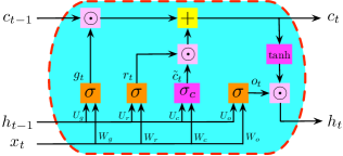
Figure 3: A building block of LSTM RNNs.

Assumption 7.

The spectral norms of weight matrices are bounded respectively, i.e. $\lVert W_{g}\rVert_{2}\leq B_{W_{g}},\lVert W_{r}\rVert_{2}\leq B_{W_{r}},\lVert W_{o}\rVert_{2}\leq B_{W_{o}},\lVert W_{c}\rVert_{2}\leq B_{W_{c}},\lVert U_{g}\rVert_{2}\leq B_{U_{g}},\lVert U_{r}\rVert_{2}\leq B_{U_{r}},\lVert U_{o}\rVert_{2}\leq B_{U_{o}},\lVert U_{h}\rVert_{2}\leq B_{U_{h}},$ and $\lVert V\rVert_{2}\leq B_{V}.$

For properly normalized weight matrices $W_{o}$ and $U_{o}$, the generalization bound of LSTM RNNs is given in the following theorem.

Theorem 5.

Let the activation operator $\sigma_{y}$ be given and Assumptions 1 and 7 hold. Then for $(x_{t},z_{t})_{t=1}^{T}$ and $S=\left\{(x_{i,t},z_{i,t})_{t=1}^{T},i=1,\dots,m\right\}$ drawn i.i.d. from any underlying distribution over $\mathbb{R}^{d_{x}\times T}\times\{1,\dots,K\}$, with probability at least $1-\delta$ over $S$, for every margin value $\gamma>0$ and every $f_{t}\in\mathcal{F}_{g,t}$ for integer $t\leq T$, we have

$$\mathbb{P}\left(\widetilde{z}_{t}\neq z_{t}\right)\leq\widehat{\mathcal{R}}_{\gamma}(f_{t})+3\sqrt{\frac{\log\frac{2}{\delta}}{2m}}+O\left(\frac{d\rho_{y}B_{V}\min\big{\{}\sqrt{d},B_{W_{c}}B_{x}\frac{\beta^{t}-1}{\beta-1}\big{\}}\sqrt{\log\big{(}\frac{\theta^{t}-1}{\theta-1}d\sqrt{m}\big{)}}}{\sqrt{m}\gamma}\right),$$

where $\beta=\max\left\{\left\lVert g_{j}\right\rVert_{\infty}+B_{U_{c}}\left\lVert r_{j}\right\rVert_{\infty}\left\lVert o_{j}\right\rVert_{\infty}\right\}$, $\theta=\beta+B_{U_{g}}+B_{U_{r}}+B_{U_{o}}$, and $d=\max\{d_{x},d_{y},d_{h}\}$.

The detailed proof is provided in Appendix C.2. Similar to MGU RNNs, LSTM RNNs also introduce extra decaying factors to reduce the dependence on $d$ and $t$ in generalization. However, LSTM RNNs are more complicated, but more flexible than MGU RNNs, since three factors, $r_{t}$, $o_{t}$ and $g_{t}$ are used to jointly control the spectrum of $U_{c}$. We further remark that LSTM RNNs need spectral norms of weight matrices, $W_{g},W_{r},W_{o},U_{g},U_{r}$ and $U_{o}$, to be properly controlled for obtaining better generalization bounds.

We further extend our analysis to Convolutional RNNs (Conv RNNs). Conv RNNs integrate convolutional filters and recurrent neural networks. Specifically, we consider input $x\in\mathbb{R}^{d}$ and $k$-channel $k$-dimensional convolutional filters $\mathcal{I}_{1},\dots,\mathcal{I}_{k}\in\mathbb{R}^{k}$ followed by an average pooling layer over the $k$ channels for reducing dimensionality. Extensions to convolution with strides and other kinds of average pooling layers (e.g., blockwise pooling) are straightforward.

Here we denote the circulant-like matrix generated by $\mathcal{I}_{i}$ as

$$C_{i}=\begin{bmatrix}\mathcal{I}_{i}^{\top}\quad~{}~{}\underbrace{0\dots\dots\dots 0}_{d-k}\\ 0\quad~{}~{}\mathcal{I}_{i}^{\top}\quad\underbrace{0\dots\dots 0}_{d-k-1}\\ ~{}~{}~{}~{}\quad\quad\quad\quad\ddots\quad\quad~{}~{}~{}~{}\\ \underbrace{0\dots\dots\dots 0}_{d-k}\quad~{}~{}\mathcal{I}_{i}^{\top}\end{bmatrix}\in\mathbb{R}^{(d-k+1)\times d},$$

and write $W_{\mathcal{I}}=[C_{1}^{\top},\dots,C_{k}^{\top}]^{\top}$. We further denote $P=\frac{1}{k}\underbrace{\left[I_{d-k+1}~{}I_{d-k+1}~{}\cdots~{}I_{d-k+1}\right]}_{\textrm{totally}~{}k~{}\textrm{identity matrices}},$ where $I_{d}$ denotes the $d$-dimensional identity matrix. Define $\mathcal{I}=[\mathcal{I}_{1},\dots,\mathcal{I}_{k}]$, and $\mathcal{I}\ast x=PW_{\mathcal{I}}x$. Given a sample $(x_{t},z_{t})_{t=1}^{T}$, the Conv RNNs compute $h_{t}$ and $y_{t}$ as follows,

$$h_{t}=\sigma_{h}\left(\mathcal{U}\ast h_{t-1}+\mathcal{W}\ast x_{t}\right),\quad\textrm{and}\quad y_{t}=\sigma_{y}\left(\mathcal{V}\ast h_{t}\right),$$

where $h_{t},x_{t}\in\mathbb{R}^{d}$, and $\mathcal{U},\mathcal{V},\mathcal{W}\in\mathbb{R}^{k\times k}$ are matrices with column vectors being $k$-dimensional convolutional filters. We use zero-padding to ensure the output dimension of convolutional filters matches the input (Krizhevsky et al., 2012). To get $y_{t}$, we convolve $h_{t}$ with $\mathcal{V}$ followed by an average pooling to reduce the dimension to $K$. Since we aim to show that Conv RNNs reduce the dependence on $d$ in generalization through parameter sharing, we simplify the notations to assume $h_{0}=0$, and impose the following assumption. Extensions to general settings are straightforward.

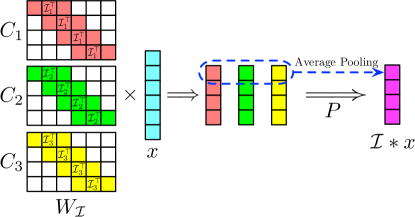
Figure 4: Illustration of input $x\in\mathbb{R}^{6}$ convolving with 3-channel 3-dimensional convolutional filters $\mathcal{I}_{1},\mathcal{I}_{2}$, and $\mathcal{I}_{3}$, followed by an average pooling.

Assumption 8.

The activation operators $\sigma_{h}$ and $\sigma_{y}$ are 1-Lipschitz with $\sigma_{h}(0)=\sigma_{y}(0)=0$. $\sigma_{h}$ is entrywise bounded by 1. The convolutional filters $\mathcal{U}$, $\mathcal{V}$, and $\mathcal{W}$ are orthogonal with normalized columns, i.e., $\mathcal{U}^{\top}\mathcal{U}=\mathcal{U}\mathcal{U}^{\top}=\frac{1}{k}I_{k},\mathcal{V}^{\top}\mathcal{V}=\mathcal{V}\mathcal{V}^{\top}=\frac{1}{k}I_{k},$ and $\mathcal{W}^{\top}\mathcal{W}=\mathcal{W}\mathcal{W}^{\top}=\frac{1}{k}I_{k}.$

We remark that the orthogonality constraints enhance the diversity among convolutional filters (Xie et al., 2017; Huang et al., 2017). Additionally, the normalization factor $\frac{1}{k}$ is to control the spectral norms of $W_{\mathcal{U}}$, $W_{\mathcal{V}}$, and $W_{\mathcal{W}}$, which prevents the blowup of hidden state. Denote by $\mathcal{F}_{c,t}$ the class of mappings from the first $t$ inputs to the $t$-th output computed by Conv RNNs. Then the generalization bound is given in the following theorem.

Theorem 6.

Let activation operators $\sigma_{h}$ and $\sigma_{y}$ be given, and Assumptions 1 and 8 hold. Then for $(x_{t},z_{t})_{t=1}^{T}$ and $S=\left\{(x_{i,t},z_{i,t})_{t=1}^{T},i=1,\dots,m\right\}$ drawn i.i.d. from any underlying distribution over $\mathbb{R}^{d\times T}\times\{1,\dots,K\}$, with probability at least $1-\delta$ over $S$, for every margin value $\gamma>0$ and every $f_{t}\in\mathcal{F}_{c,t}$ for integer $t\leq T$, we have

$$\mathbb{P}\left(\widetilde{z}_{t}\neq z_{t}\right)\leq\widehat{\mathcal{R}}_{\gamma}(f_{t})+O\left(\frac{kt\sqrt{\log\left(dt\sqrt{m}\right)}}{\sqrt{m}\gamma}+\sqrt{\frac{\log\frac{1}{\delta}}{m}}\right).$$

The detailed proof is provided in C.3. Similar to the analysis of vanilla RNNs, our proof is based on the Lipschitz continuity of Conv RNNs with respect to its model parameters in the convolutional filters. Specifically, by Assumption 8, the spectral norms of $W_{\mathcal{U}}$, $W_{\mathcal{V}}$, and $W_{\mathcal{W}}$ are all bounded by 1. Combining with the inequality, $\|W_{\mathcal{U}}\|_{\textrm{F}}\leq\sqrt{d}\|\mathcal{U}\|_{\textrm{F}}$, we have $\lVert y_{t}-y^{\prime}_{t}\rVert_{2}\leq L_{V,t}\lVert\mathcal{V}-\mathcal{V}^{\prime}\rVert_{\textrm{F}}+L_{\mathcal{U},t}\lVert\mathcal{U}-\mathcal{U}^{\prime}\rVert_{\textrm{F}}+L_{\mathcal{W},t}\lVert\mathcal{W}-\mathcal{W}^{\prime}\rVert_{\textrm{F}},$ where $L_{\mathcal{U},t}$, $L_{\mathcal{V},t}$, and $L_{\mathcal{W},t}$ are polynomials in $d$ and $t$. Additionally, observe that the total number of parameters in a Conv RNN is at most $3k^{2}$, which is independent of input dimension $d$. As a consequence, the generalization bound of Conv RNNs only has a lieanr dependence on $k$ and $t$.

6 Numerical Evaluation

We demonstrate a comparison among our obtained generalization bound with Bartlett et al. (2017), Neyshabur et al. (2017), and Zhang et al. (2018). Specifically, we train a vanilla RNN on the wikitext language modeling dataset (Merity et al., 2016). We take $\sigma_{h}=\tanh$ and set the hidden state $h\in\mathbb{R}^{128}$ and the input $x\in\mathbb{R}^{14}$ with $\|x\|_{2}\leq 1$. Accordingly, we have $d=128$ and take the sequence length $t=56$. We list the complexity bounds for vanilla RNNs in Theorem 2 (Ours), Zhang et al. (2018) (Bound 1), (2) of Theorem 3 (Bound 2), and (3) of Theorem 3 (Bound 3) neglecting common log factors in $d$ and $t$:

• Ours: $dB_{V}\min\big{\{}\sqrt{d},B_{W}\frac{B_{U}^{t}-1}{B_{U}-1}\big{\}}\sqrt{\log\big{(}\frac{B_{U}^{t}-1}{B_{U}-1}\big{)}}$;

• Bound 1: $dt^{2}B_{V}B_{W}\max\{1,B_{U}^{t}\}$;

• Bound 2: $B_{V}B_{W}\left(M_{U}+M_{V}+M_{W}\right)t\frac{B_{U}^{t}-1}{B_{U}-1}$;

• Bound 3: $\big{(}\min\{\sqrt{d},B_{W}\frac{B_{U}^{t}-1}{B_{U}-1}\}B_{U}+B_{W}\big{)}\frac{B_{U}^{t}-1}{B_{U}-1}\times\sqrt{d(B_{U,\textrm{F}}^{2}+B_{W,\textrm{F}}^{2}+B_{V,\textrm{F}}^{2})}.$

The corresponding complexity bounds are shown in Figure 5. As can be seen, our complexity bound in Theorem 2 is much smaller than Bounds 1-3. In more detail, the trained vanilla RNN has $B_{U}=2.6801>1$. As discussed earlier, for $B_{U}>1$, only our bound in Theorem 2 is polynomial in the size of the network, while Bounds 1-3 are all exponential in $t$. The resulting complexity bounds corroborate such a conclusion.

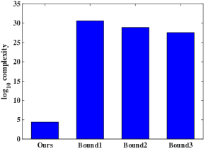
Figure 5: Complexity bounds on wikitext dataset.

We also observe that Bound 3 is smaller than Bound 2. The reason behind is that the weight matrices in the trained vanilla RNN have relatively small Frobenius norms but large $(2,1)$ norms. Taking matrix $U$ as an example, we have $B_{U,\textrm{F}}=13.6823$ and $M_{U}=154.5439$. Then, we can calculate the stable rank $\frac{B_{U,\textrm{F}}}{B_{U}}=5.1<\sqrt{d}/2$, and the ratio $\frac{M_{U}}{B_{U,\textrm{F}}}=11.3\approx\sqrt{d}$. This implies that the singular values of $U$ are not evenly distributed, while the norms of row vectors in $U$ are approximately equal.

7 Discussions and Open Problems

(I) Tighter bounds: Our obtained generalization bounds depend on the spectral norms of weight matrices and the network size. Can we exploit other modeling structures to further reduce the dependence on the network size? Or can we find better choices of norms of weight matrices that yield better bounds?

(II) Margin value: Our generalization bounds depend on the margin value of the predictors. As can be seen, a larger margin value yields a better generalization bound. However, establishing a sharp characterization of the margin value is technically very challenging, because of its complicated dependence on the underlying data distribution and the training algorithm.

(III) Implicit bias of SGD: Numerous empirical evidences have already shown that RNNs trained by stochastic gradient descent (SGD) algorithms have superior generalization performance. There have been a few theoretical results showing that SGD tends to yield low complexity models, which can generalize (Neyshabur et al., 2014, 2015; Zhang et al., 2016; Soudry et al., 2017). Can we extend this argument to RNNs? For example, can SGD always yield weight matrices with well controlled spectra? This is crucial to the generalization of MGU and LSTM RNNs.

(IV) Adaptivity to the underlying distribution: The current PAC-Learning framework focuses on the worst case. Taking classification as an example, the theoretical analysis holds even when the input features and labels are completely independent. Therefore, this often yields very pessimistic results. For many real applications, however, data are not obtained adversarially. Some recent empirical evidences suggest that the generalization of neural networks seems very adaptive to the underlying distribution: Easier tasks lead to low complexity neural networks, while harder ones lead to highly complex neural networks. Unfortunately, none of the existing analysis can take the underlying distribution into consideration.

(V) Sequentially dependent data: To extend the analysis to scenarios where input sequences are dependent is quite challenging and largely open. Rakhlin et al. (2015) propose a so-called “Sequential Rademacher Complexity” to quantify the model complexity with dependent data. Their bound however, is exponential in the depth of a neural network, even with proper normalization on the weight matrices. Kuznetsov and Mohri (2017) also derive generalization bounds for dependent data under mixing conditions. They assume block independence for a sub-sample selection trick. The extension to fully dependent data is beyond the scope of this paper. We leave it for future investigation.

Appendix A Proofs in Section 2

A.1 Lipschitz Continuity of $\mathcal{M}$ and $\ell_{\gamma}$

We show the Lipschitz continuity of the margin operator $\mathcal{M}$ and the loss function $\ell_{\gamma}$ in the following lemma.

Lemma 5.

The margin operator $\mathcal{M}$ is 2-Lipschitz in its first argument with respect to vector Euclidean norm, and $\ell_{\gamma}$ is $\frac{1}{\gamma}$-Lipschitz.

Proof.

Let $y$, $y^{\prime}$ and $z$ be given, then

$$\bigg{|}\mathcal{M}(y,z)-\mathcal{M}\left(y^{\prime},z\right)\bigg{|} =\bigg{|}y_{z}-y^{\prime}_{z}+\left(\max_{j\neq z}y^{\prime}_{j}-\max_{j\neq z}y_{j}\right)\bigg{|}$$

$$\leq\bigg{|}y_{z}-y^{\prime}_{z}\bigg{|}+\bigg{|}\max_{j\neq z}y^{\prime}_{j}-y_{j}\bigg{|}$$

$$\leq 2\left\lVert y-y^{\prime}\right\rVert_{\infty}\leq\left\lVert y-y^{\prime}\right\rVert_{2}.$$

For function $\ell_{\gamma}$, it is a piecewise linear function. Thus, it is straightforward to see that $\ell_{\gamma}$ is $\frac{1}{\gamma}$-Lipschitz. ∎

A.2 Proof of Lemma 2

Proof.

The Lemma is stated with matrix Frobenius norms. However, we can show a tighter bound only involving the spectral norms of weight matrices. Given weight matrices $U,V,W$ and $U^{\prime},V^{\prime},W^{\prime}$, consider the $t$-th outputs $y_{t}$ and $y^{\prime}_{t}$ of vanilla RNNs,

$$\left\lVert y_{t}-y^{\prime}_{t}\right\rVert_{2} =\left\lVert\sigma_{y}(Vh_{t})-\sigma_{y}(V^{\prime}h^{\prime}_{t})\right\rVert_{2}$$

$$\leq\rho_{y}\left\lVert Vh_{t}-V^{\prime}h_{t}+V^{\prime}h_{t}-V^{\prime}h^{\prime}_{t}\right\rVert_{2}$$

$$\leq\rho_{y}\left(\left\lVert(V-V^{\prime})h_{t}\right\rVert_{2}+\left\lVert V^{\prime}(h_{t}-h^{\prime}_{t})\right\rVert_{2}\right)$$

$$\leq\rho_{y}\left(\left\lVert h_{t}\right\rVert_{2}\left\lVert V-V^{\prime}\right\rVert_{2}+B_{V}\left\lVert h_{t}-h^{\prime}_{t}\right\rVert_{2}\right).$$ (4)

We have to bound the norm of $h_{t}$ as in the following lemma.

Lemma 6.

Under Assumptions 1 to 3, for $t\geq 0$, the norm of $h_{t}$ is bounded by

$$\left\lVert h_{t}\right\rVert_{2}\leq\min\left\{b\sqrt{d},\rho_{h}B_{W}B_{x}\frac{\left(\rho_{h}B_{U}\right)^{t}-1}{\rho_{h}B_{U}-1}\right\}.$$ (5)

Proof.

We prove by induction. Observe that for $t\geq 1$, we have

$$\left\lVert h_{t}\right\rVert_{2} =\left\lVert\sigma_{h}(Wx_{t}+Uh_{t-1})\right\rVert_{2}$$

$$\leq\rho_{h}\left\lVert Wx_{t}+Uh_{t-1}\right\rVert_{2}$$

$$\leq\rho_{h}\left(\left\lVert Wx_{t}\right\rVert_{2}+\left\lVert Uh_{t-1}\right\rVert_{2}\right)$$

$$\leq\rho_{h}\left(B_{W}B_{x}+B_{U}\left\lVert h_{t-1}\right\rVert_{2}\right).$$ (6)

Applying equation (6) recursively with $h_{0}=0$, we arrive at,

$$\left\lVert h_{t}\right\rVert_{2}\leq\rho_{h}B_{W}B_{x}\sum_{j=0}^{t-1}(\rho_{h}B_{U})^{j}=\rho_{h}B_{W}B_{x}\frac{\left(\rho_{h}B_{U}\right)^{t}-1}{\rho_{h}B_{U}-1},$$

We also have $\lVert h_{t}\rVert_{\infty}\leq b$. Thus, combining with the above upper bound, we get

$$\left\lVert h_{t}\right\rVert_{2}\leq\min\left\{b\sqrt{d},\rho_{h}B_{W}B_{x}\frac{\left(\rho_{h}B_{U}\right)^{t}-1}{\rho_{h}B_{U}-1}\right\}.$$

Clearly, $\lVert h_{0}\rVert_{2}=0$ satisfies the upper bound. ∎

When $\rho_{h}B_{U}=1$, the ratio is defined, by L’Hospital’s rule, to be the limit,

$$\lim_{\rho_{h}B_{U}\rightarrow 1}\frac{(\rho_{h}B_{U})^{t}-1}{\rho_{h}B_{U}-1}=t.$$

With Lemma 6 in hand, we plug the bound (5) into equation (4) and end up with

$$\left\lVert y_{t}-y^{\prime}_{t}\right\rVert_{2}\leq\rho_{y}\rho_{h}B_{W}B_{x}\frac{\left(\rho_{h}B_{U}\right)^{t}-1}{\rho_{h}B_{U}-1}\left\lVert V-V^{\prime}\right\rVert_{2}+\rho_{y}B_{V}\left\lVert h_{t}-h^{\prime}_{t}\right\rVert_{2}.$$ (7)

The remaining task is to bound $\left\lVert h_{t}-h^{\prime}_{t}\right\rVert_{2}$ in terms of the spectral norms of the difference of weight matrices, $\left\lVert W-W^{\prime}\right\rVert_{2}$ and $\left\lVert U-U^{\prime}\right\rVert_{2}$.

Lemma 7.

Under Assumptions 1 to 3, for $t\geq 1$, the difference of hidden states $h_{t}$ and $h^{\prime}_{t}$ satisfies

$$\left\lVert h_{t}-h^{\prime}_{t}\right\rVert_{2}\leq L_{W,t}\left\lVert W-W^{\prime}\right\rVert_{2}+L_{U,t}\left\lVert U-U^{\prime}\right\rVert_{2},$$

where $L_{W,t}=\rho_{h}B_{x}\frac{(\rho_{h}B_{U})^{t}-1}{\rho_{h}B_{U}-1}$ and $L_{U,t}=\rho_{h}^{2}B_{W}B_{x}t\frac{(\rho_{h}B_{U})_{2}^{t}-1}{(\rho_{h}B_{U})-1}$.

Proof.

Similar to the proof of Lemma 6, we use induction.

$$\left\lVert h_{t}-h^{\prime}_{t}\right\rVert_{2} =\left\lVert\sigma_{h}\left(Wx_{t}+Uh_{t-1}\right)-\sigma_{h}\left(W^{\prime}x_{t}+U^{\prime}h^{\prime}_{t-1}\right)\right\rVert_{2}$$

$$\leq\rho_{h}\left\lVert(W-W^{\prime})x_{t}+Uh_{t-1}-U^{\prime}h^{\prime}_{t-1}\right\rVert_{2}$$

$$\leq\rho_{h}\left(\left\lVert(W-W^{\prime})x_{t}\right\rVert_{2}+\left\lVert Uh_{t-1}-U^{\prime}h^{\prime}_{t-1}\right\rVert_{2}\right)$$

$$\leq\rho_{h}\left(B_{x}\left\lVert W-W^{\prime}\right\rVert_{2}+\left\lVert Uh_{t-1}-U^{\prime}h_{t-1}+U^{\prime}h_{t-1}-U^{\prime}h^{\prime}_{t-1}\right\rVert_{2}\right)$$

$$\leq\rho_{h}B_{x}\left\lVert W-W^{\prime}\right\rVert_{2}+\rho_{h}\left(\left\lVert h_{t-1}\right\rVert_{2}\left\lVert U-U^{\prime}\right\rVert_{2}+B_{U}\left\lVert h_{t-1}-h^{\prime}_{t-1}\right\rVert_{2}\right).$$

Repeat this derivation recursively, we have

$$\left\lVert h_{t}-h^{\prime}_{t}\right\rVert_{2} \leq\rho_{h}B_{x}\left\lVert W-W^{\prime}\right\rVert_{2}+\rho_{h}\left\lVert h_{t-1}\right\rVert_{2}\left\lVert U-U^{\prime}\right\rVert_{2}+\rho_{h}B_{U}\left\lVert h_{t-1}-h^{\prime}_{t-1}\right\rVert_{2}$$

$$\leq\rho_{h}B_{x}\left(1+\rho_{h}B_{U}\right)\left\lVert W-W^{\prime}\right\rVert_{2}+\rho_{h}\left(\left\lVert h_{t-1}\right\rVert_{2}+\rho_{h}B_{U}\left\lVert h_{t-2}\right\rVert_{2}\right)\left\lVert U-U^{\prime}\right\rVert_{2}$$

$$\hskip 14.45377pt+\left(\rho_{h}B_{U}\right)^{2}\left\lVert h_{t-2}-h^{\prime}_{t-2}\right\rVert_{2}$$

$$\leq\dots\dots$$

$$\leq\rho_{h}B_{x}\sum_{j=0}^{t-1}\left(\rho_{h}B_{U}\right)^{j}\left\lVert W-W^{\prime}\right\rVert_{2}+\rho_{h}\sum_{j=0}^{t-1}\left((\rho_{h}B_{U})^{t-1-j}\left\lVert h_{j}\right\rVert_{2}\right)\left\lVert U-U^{\prime}\right\rVert_{2}$$

$$\hskip 14.45377pt+(\rho_{h}B_{U})^{t}\left\lVert h_{0}-h^{\prime}_{0}\right\rVert_{2}$$

$$\leq\rho_{h}B_{x}\frac{(\rho_{h}B_{U})^{t}-1}{\rho_{h}B_{U}-1}\left\lVert W-W^{\prime}\right\rVert_{2}+\rho_{h}\sum_{j=0}^{t-1}\left((\rho_{h}B_{U})^{t-1-j}\left\lVert h_{j}\right\rVert_{2}\right)\left\lVert U-U^{\prime}\right\rVert_{2}.$$ (8)

We now plug in the upper bound (5) to calculate the summation involving the Euclidean norms of the hidden state $h_{t}$.

$$\sum_{j=0}^{t-1}(\rho_{h}B_{U})^{t-1-j}\left\lVert h_{j}\right\rVert_{2} \leq\sum_{j=0}^{t-1}(j+1)(\rho_{h}B_{U})^{j}\rho_{h}B_{W}B_{x}\leq t\sum_{j=0}^{t-1}(\rho_{h}B_{U})^{j}\rho_{h}B_{W}B_{x}$$

$$\leq\rho_{h}B_{W}B_{x}t\frac{(\rho_{h}B_{U})^{t}-1}{\rho_{h}B_{U}-1}.$$

Plugging back into equation (8), we have as desired,

$$\left\lVert h_{t}-h^{\prime}_{t}\right\rVert_{2}\leq\rho_{h}B_{x}\frac{(\rho_{h}B_{U})^{t}-1}{\rho_{h}B_{U}-1}\left\lVert W-W^{\prime}\right\rVert_{2}+\rho_{h}^{2}B_{W}B_{x}t\frac{(\rho_{h}B_{U})^{t}-1}{\rho_{h}B_{U}-1}\left\lVert U-U^{\prime}\right\rVert_{2}.$$

∎

Combining equation (7) and Lemma 7, and $\|W\|_{\textrm{F}}\geq\|W\|_{2}$, we immediately get Lemma 2. ∎

A.3 Proof of Lemma 3

Proof.

Our goal is to construct a covering $\mathcal{C}(\mathcal{F}_{t},\epsilon,\textrm{dist}(\cdot,\cdot))$, i.e., for any $f_{t}\in\mathcal{F}_{t}$, there exists $\widehat{f}_{t}\in\mathcal{F}_{t}$, for any input data $(x_{t})_{t=1}^{T}$, satisfying

$$\sup_{X_{t}}\left\lVert f_{t}(X_{t})-\widehat{f}_{t}(X_{t})\right\rVert_{2}\leq\epsilon.$$

Note that $f$ is determined by weight matrices $U,V$ and $W$. By Lemma 2, we have

$$\sup_{X_{t}}\left\lVert f(X_{t})-\widehat{f}_{t}(X_{t})\right\rVert_{2}\leq L_{V,t}\left\lVert V-\widehat{V}\right\rVert_{\textrm{F}}+L_{W,t}\left\lVert W-\widehat{W}\right\rVert_{\textrm{F}}+L_{U,t}\left\lVert U-\widehat{U}\right\rVert_{\textrm{F}}.$$

Then it is enough to construct three matrix coverings, $\mathcal{C}\left(U,\frac{\epsilon}{3L_{U,t}},\lVert\cdot\rVert_{\textrm{F}}\right)$, $\mathcal{C}\left(V,\frac{\epsilon}{3L_{V,t}},\lVert\cdot\rVert_{\textrm{F}}\right)$ and $\mathcal{C}\left(W,\frac{\epsilon}{3L_{W,t}},\lVert\cdot\rVert_{\textrm{F}}\right)$. Their Cartesian product gives us the covering $\mathcal{C}(\mathcal{F}_{t},\epsilon,\textrm{dist}(\cdot,\cdot))$. The following lemma gives an upper bound on the covering number of matrices with a bounded Frobenius norm.

Lemma 8.

Let $\mathcal{G}=\left\{A\in\mathbb{R}^{d_{1}\times d_{2}}:\lVert A\rVert_{2}\leq\lambda\right\}$ be the set of matrices with bounded spectral norm and $\epsilon>0$ be given. The covering number $\mathcal{N}(\mathcal{G},\epsilon,\lVert\cdot\rVert_{\textrm{F}})$ is upper bounded by

$$\mathcal{N}(\mathcal{G},\epsilon,\lVert\cdot\rVert_{\textrm{F}})\leq\left(1+2\frac{\min\left\{\sqrt{d_{1}},\sqrt{d_{2}}\right\}\lambda}{\epsilon}\right)^{d_{1}d_{2}}.$$

Proof.

For any matrix $A\in\mathcal{G}$, we define a mapping $\phi:\mathbb{R}^{d_{1}\times d_{2}}\mapsto\mathbb{R}^{d_{1}d_{2}}$, such that $\phi(A)=[A_{:,1}^{\top},A_{:,2}^{\top},\dots,A_{:,h}^{\top}]^{\top}$, where $A_{:,i}$ denotes the $i$-th column of matrix $A$. Denote the vector space induced by the mapping $\phi$ by $\mathcal{V}(\mathcal{G})=\left\{\phi(A):A\in\mathcal{G}\right\}$. Note that we have $\lVert A\rVert_{\textrm{F}}^{2}=\sum_{i=1}^{h}A_{:,i}^{\top}A_{:,i}=\lVert\phi(A)\rVert_{2}^{2}$ and the mapping $\phi$ is one-to-one and onto. By definition, the square of Frobenius norm equals the square of sum of singular values and the spectral norm is the largest singular value. Hence, the equivalence of Frobenius norm and spectral norm is given by the following inequalities,

$$\lVert A\rVert_{2}\leq\lVert A\rVert_{\textrm{F}}\leq\min\left\{\sqrt{d_{1}},\sqrt{d_{2}}\right\}\lVert A\rVert_{2}.$$

Now, we see that if we construct a covering $\mathcal{C}(\mathcal{V}(\mathcal{G}),\epsilon,\lVert\cdot\rVert_{2})$, then

$$\phi^{-1}\mathcal{C}(\mathcal{V}(\mathcal{G}),\epsilon,\lVert\cdot\rVert_{2})=\left\{\phi^{-1}(v):v\in\mathcal{C}(\mathcal{V}(\mathcal{G}),\epsilon,\lVert\cdot\rVert_{2})\right\}$$

is a covering of $\mathcal{G}$ at scale $\epsilon$ with respect to the matrix Frobenius norm. Therefore, we get

$$\mathcal{N}(\mathcal{G},\epsilon,\lVert\cdot\rVert_{\textrm{F}})\leq\mathcal{N}(\mathcal{V}(\mathcal{G}),\epsilon,\lVert\cdot\rVert_{2}).$$

As a consequence, it is suffices to upper bound the covering number of $\mathcal{V}(\mathcal{G})$. In order to do so, we need another closely related concept, packing number.

Definition 2 (Packing).

Let $\mathcal{G}$ be an arbitrary set and $\epsilon>0$ be given. We say $\mathcal{P}(\mathcal{G},\epsilon,\lVert\cdot\rVert)$ is a packing of $\mathcal{G}$ at scale $\epsilon$ with respect to the norm $\lVert\cdot\rVert$, if for any two elements $A,B\in\mathcal{P}$, we have

$$\left\lVert A-B\right\rVert>\epsilon.$$

Denote by $\mathcal{M}(\mathcal{G},\epsilon,\lVert\cdot\rVert)$ the maximal cardinality of $\mathcal{P}(\mathcal{G},\epsilon,\lVert\cdot\rVert)$.

By the maximality, we can check that $\mathcal{N}(C,\epsilon,\lVert\cdot\rVert)\leq\mathcal{M}(C,\epsilon,\lVert\cdot\rVert)$. Indeed, let $\mathcal{P}^{*}(\mathcal{G},\epsilon,\lVert\cdot\rVert)$ be a maximal packing. Suppose there exists $A\in\mathcal{G}$ such that for any $B\in\mathcal{P}^{*}(\mathcal{G},\epsilon,\lVert\cdot\rVert)$, the inequality $\left\lVert A-B\right\rVert>\epsilon$ holds. Then we can add $A$ to $\mathcal{P}^{*}(\mathcal{G},\epsilon,\lVert\cdot\rVert)$, while still keeping it being a packing, which contradicts the maximality of $\mathcal{P}^{*}(\mathcal{G},\epsilon,\lVert\cdot\rVert)$. Thus, we have $\mathcal{N}(\mathcal{G},\epsilon,\lVert\cdot\rVert)\leq\mathcal{M}(\mathcal{G},\epsilon,\lVert\cdot\rVert)$.

Observe that $\mathcal{V}(\mathcal{G})$ is contained in an Euclidean ball $\mathcal{B}(0;R)\in\mathbb{R}^{d_{1}d_{2}}$ of radius at most

$$R=\max_{A\in\mathcal{G}}\lVert\phi(A)\rVert_{2}\leq\min\left\{\sqrt{d_{1}},\sqrt{d_{2}}\right\}\lVert A\rVert_{2}\leq\min\left\{\sqrt{d_{1}},\sqrt{d_{2}}\right\}\lambda.$$

Additionally, the union of Euclidean balls $\mathcal{B}(v;\epsilon/2)\subset\mathbb{R}^{d_{1}d_{2}}$ with radius $\epsilon/2$ and center $v\in\mathcal{P}(\mathcal{V}(\mathcal{G}),\epsilon,\lVert\cdot\rVert_{2})$ is further contained in an Euclidean ball $\mathcal{B}(0;R_{\epsilon})$ of slightly enlarged radius $R_{\epsilon}=\min\left\{\sqrt{d_{1}},\sqrt{d_{2}}\right\}\lambda+\epsilon/2$. Those balls $\mathcal{B}(v;\epsilon/2)$ are disjoint by the definition of packing, thus we have

$$\mathcal{N}(\mathcal{V}(C),\epsilon,\lVert\cdot\rVert_{2}) \leq\mathcal{P}(\mathcal{V}(C),\epsilon,\lVert\cdot\rVert_{2})\leq\frac{\textrm{vol}(\mathcal{B}(0,R_{\epsilon}))}{\textrm{vol}(\mathcal{B}(v;\epsilon/2))}=\left(\frac{R_{\epsilon}}{\epsilon/2}\right)^{d_{1}d_{2}}$$

$$=\left(1+2\frac{\min\{\sqrt{d_{1}},\sqrt{d_{2}}\}\lambda}{\epsilon}\right)^{d_{1}d_{2}},$$

where $\textrm{vol}(\cdot)$ denotes the volume. ∎

By Lemma 8, we can directly write out the upper bounds on the covering numbers of weight matrices,

$$\mathcal{N}\left(U,\frac{\epsilon}{3L_{U,t}},\lVert\cdot\rVert_{\textrm{F}}\right)\leq\left(1+6\frac{\sqrt{d_{h}}B_{U}L_{U,t}}{\epsilon}\right)^{d_{h}^{2}},$$

$$\mathcal{N}\left(V,\frac{\epsilon}{3L_{V,t}},\lVert\cdot\rVert_{\textrm{F}}\right)\leq\left(1+6\frac{\min\{\sqrt{d_{y}},\sqrt{d_{h}}\}B_{V}L_{V,t}}{\epsilon}\right)^{d_{y}d_{h}},\quad\textrm{and}$$

$$\mathcal{N}\left(W,\frac{\epsilon}{3L_{W,t}},\lVert\cdot\rVert_{\textrm{F}}\right)\leq\left(1+6\frac{\min\{\sqrt{d_{x}},\sqrt{d_{h}}\}B_{W}L_{W,t}}{\epsilon}\right)^{d_{x}d_{h}}.$$

Then we immediately have,

$$\mathcal{N}(\mathcal{F}_{t},\epsilon,\textrm{dist}(\cdot,\cdot)) \leq\mathcal{N}\left(U,\frac{\epsilon}{3L_{U,t}},\lVert\cdot\rVert_{\textrm{F}}\right)\times\mathcal{N}\left(V,\frac{\epsilon}{3L_{V,t}},\lVert\cdot\rVert_{\textrm{F}}\right)\times\mathcal{N}\left(W,\frac{\epsilon}{3L_{W,t}},\lVert\cdot\rVert_{\textrm{F}}\right)$$

$$\leq\left(1+\frac{6\sqrt{d_{h}}B_{U}L_{U,t}}{\epsilon}\right)^{d_{h}^{2}}\left(1+\frac{\min\{6\sqrt{d_{y}},\sqrt{d_{h}}\}B_{V}L_{V,t}}{\epsilon}\right)^{d_{y}d_{h}}$$

$$~{}~{}\times\left(1+\frac{6\min\{\sqrt{d_{x}},\sqrt{d_{h}}\}B_{W}L_{W,t}}{\epsilon}\right)^{d_{x}d_{h}}.$$

Substituting the coefficients $L_{U,t},L_{V,t}$ and $L_{W,t}$ from Lemma 2, we get

$$\mathcal{N}(\mathcal{F}_{t},\epsilon,\textrm{dist}(\cdot,\cdot))$$

$$\leq\left(1+\frac{6\sqrt{d}\rho_{y}\rho_{h}B_{V}B_{W}B_{x}\frac{(\rho_{h}B_{U})^{t}-1}{\rho_{h}B_{U}-1}}{\epsilon}\right)^{2d^{2}}\left(1+\frac{6\sqrt{d}\rho_{y}\rho_{h}^{2}B_{U}B_{V}B_{W}B_{x}t\frac{(\rho_{h}B_{U})^{t}-1}{\rho_{h}B_{U}-1}}{\epsilon}\right)^{d^{2}}$$

$$\leq\left(1+\frac{6c\sqrt{d}t\frac{(\rho_{h}B_{U})^{t}-1}{\rho_{h}B_{U}-1}}{\epsilon}\right)^{3d^{2}},$$

where $c=\rho_{y}\rho_{h}B_{V}B_{W}B_{x}\max\left\{1,\rho_{h}B_{U}\right\}$. For future usage, we also write down for small $\epsilon>0$, such that $\frac{6c\sqrt{d}t\frac{(\rho_{h}B_{U})^{t}-1}{\rho_{h}B_{U}-1}}{\epsilon}>1$, the logarithm of covering number satisfies,

$$\log\mathcal{N}(\mathcal{F}_{t},\epsilon,\textrm{dist}(\cdot,\cdot))\leq 3d^{2}\log\left(\frac{12c\sqrt{d}t\frac{(\rho_{h}B_{U})^{t}-1}{\rho_{h}B_{U}-1}}{\epsilon}\right).$$

∎

A.4 Proof of Lemma 4

Proof.

Define $\mathcal{F}_{\mathcal{M},t}=\left\{(X_{t},z_{t})\mapsto\mathcal{M}(f_{t}(X_{t}),z_{t}):f_{t}\in\mathcal{F}_{t}\right\}$. By Lemma 5, we see that $\mathcal{M}$ is 2-Lipschitz in its first argument. In order to cover $\mathcal{F}_{\mathcal{M},t}$ at scale $\epsilon$, it suffices to cover $\mathcal{F}_{t}$ at scale $\frac{\epsilon}{2}$. This immediately gives us the covering number $\mathcal{N}(\mathcal{F}_{\mathcal{M},t},\epsilon,\lVert\cdot\rVert_{\infty})\leq\mathcal{N}(\mathcal{F}_{t},\epsilon/2,\textrm{dist}(\cdot,\cdot))$.

We then give the statement of Dudley’s entropy integral.

Lemma 9.

Let $\mathcal{H}$ be a real-valued function class taking values in $[-r,r]$ for some constant $r$, and assume that $0\in\mathcal{H}$. Let $S=(s_{1},\dots,s_{m})$ be given points, then

$$\mathfrak{R}_{S}(\mathcal{H})\leq\inf_{\alpha>0}\left(\frac{4\alpha}{\sqrt{m}}+\frac{12}{m}\int_{\alpha}^{2r\sqrt{m}}\sqrt{\log\mathcal{N}(\mathcal{H},\epsilon,\lVert\cdot\rVert)}d\epsilon\right).$$

The proof can be found in Bartlett et al. (2017). Taking $\mathcal{H}=\mathcal{F}_{\mathcal{M},t}$, we can easily verify that $\mathcal{F}_{\mathcal{M},t}$ takes values in $[-r,r]$ with $r=\rho_{y}B_{V}\lVert h_{t}\rVert_{2}\leq\rho_{y}B_{V}\min\left\{b\sqrt{d},\rho_{h}B_{W}B_{x}\frac{(\rho_{h}B_{U})^{t}-1}{\rho_{h}B_{U}-1}\right\}$ and $0\in\mathcal{F}_{\mathcal{M}}$. Thus, directly applying Lemma 9 yields the following bound,

$$\mathfrak{R}_{S}(\mathcal{F}_{\mathcal{M},t})\leq\inf_{\alpha>0}\left(\frac{4\alpha}{\sqrt{m}}+\frac{12}{m}\int_{\alpha}^{2r\sqrt{m}}\sqrt{\log\mathcal{N}(\mathcal{F}_{\mathcal{M},t},\epsilon,\lVert\cdot\rVert_{\infty})}d\epsilon\right).$$

We bound the integral as follows,

$$\int_{\alpha}^{2r\sqrt{m}}\sqrt{\log\mathcal{N}(\mathcal{F}_{\mathcal{M},t},\epsilon,\lVert\cdot\rVert_{\infty})}d\epsilon \leq\int_{\alpha}^{2r\sqrt{m}}\sqrt{3d^{2}\log\left(\frac{24c\sqrt{d}t\frac{(\rho_{h}B_{U})^{t}-1}{\rho_{h}B_{U}-1}}{\epsilon}\right)}d\epsilon$$

$$\leq 2r\sqrt{m}\sqrt{3d^{2}\log\left(\frac{24c\sqrt{d}t\frac{(\rho_{h}B_{U})^{t}-1}{\rho_{h}B_{U}-1}}{\alpha}\right)}.$$

Picking $\alpha=\frac{1}{\sqrt{m}}$ is enough to give us an upper bound on $\mathfrak{R}_{S}(\mathcal{F}_{\mathcal{M},t})$,

$$\mathfrak{R}_{S}(\mathcal{F}_{\mathcal{M}})\leq\frac{4}{m}+\frac{24}{\sqrt{m}}\sqrt{3d^{2}r^{2}\log\left(24c\sqrt{dm}t\frac{(\rho_{h}B_{U})^{t}-1}{\rho_{h}B_{U}-1}\right)}.$$

Finally, by Talagrand’s lemma (Mohri et al., 2012) and $\mathcal{L}_{\gamma}$ being $\frac{1}{\gamma}$-Lipschitz, we have

$$\mathfrak{R}_{S}(\mathcal{F}_{\gamma,t})\leq\frac{1}{\gamma}\mathfrak{R}_{S}(\mathcal{F}_{\mathcal{M},t})\leq\frac{4}{m\gamma}+\frac{24}{\sqrt{m}\gamma}\sqrt{3d^{2}r^{2}\log\left(24c\sqrt{dm}t\frac{(\rho_{h}B_{U})^{t}-1}{\rho_{h}B_{U}-1}\right)}.$$

∎

Appendix B Proof in Section 4

B.1 Proof of Theorem 3

Proof.

Under additional Assumption 4, we only need to show that, with the additional matrix induced norm bound, we have a refined upper bound on the matrix covering number. The proof relies on the following lemma adapted from Bartlett et al. (2017) Lemma 3.2.

Lemma 10.

Let $\mathcal{G}=\left\{A\in\mathbb{R}^{d_{1}\times d_{2}}:\|A\|_{2,1}\leq\lambda\right\}$. We have the following matrix covering upper bound

$$\log\mathcal{N}(\mathcal{G},\epsilon,\|\cdot\|_{2})\leq\frac{\lambda^{2}}{\epsilon^{2}}\log(2d_{1}d_{2}).$$

The above Lemma is a direct consequence of Lemma 3.2 in Bartlett et al. (2017) with $X$ being identity, $a=\lambda$, $b=1$, and $m=d_{1},d=d_{2}$. We apply the same trick to split the overall covering accuracy $\epsilon$ into 3 parts, $\frac{\epsilon}{3L_{U,t}}$, $\frac{\epsilon}{3L_{V,t}}$, and $\frac{\epsilon}{3L_{W,t}}$, corresponding to $U,V,W$ respectively. Then we derive a refined bound on the covering number of $\mathcal{F}_{t}$:

$$\log\mathcal{N}(\mathcal{F}_{t},\epsilon,\textrm{dist}(\cdot,\cdot))\leq\frac{9\left(M_{U}L^{2}_{U,t}+M_{V}L^{2}_{V,t}+M_{W}L^{2}_{W,t}\right)}{\epsilon^{2}}\log(2d^{2}),$$ (9)

where $d=\max\left\{d_{x},d_{y},d_{h}\right\}$. Substituting (9) into the Dudley integral as in the proof of Lemma 4 yields

$$\mathfrak{R}_{S}(\mathcal{F}_{\mathcal{M},t})\leq\inf_{\alpha>0}\left(\frac{4\alpha}{\sqrt{m}}+\frac{12}{m}\int_{\alpha}^{2r\sqrt{m}}\sqrt{\log\mathcal{N}(\mathcal{F}_{t},\epsilon/2,\lVert\cdot\rVert_{\infty})}d\epsilon\right).$$

We bound the integral as follows,

$$\int_{\alpha}^{2r\sqrt{m}}\sqrt{\log\mathcal{N}(\mathcal{F}_{t},\epsilon/2,\lVert\cdot\rVert_{\infty})}d\epsilon \leq\int_{\alpha}^{2r\sqrt{m}}36\frac{\sqrt{M_{U}L^{2}_{U,t}+M_{V}L^{2}_{V,t}+M_{W}L^{2}_{W,t}}}{\epsilon}\sqrt{\log(2d^{2})}d\epsilon$$

$$=36\sqrt{M_{U}L^{2}_{U,t}+M_{V}L^{2}_{V,t}+M_{W}L^{2}_{W,t}}\sqrt{\log(2d^{2})}\log\frac{2r\sqrt{m}}{\alpha}.$$

Choosing $\alpha=\frac{1}{\sqrt{m}}$ yields

$$\mathfrak{R}_{S}(\mathcal{F}_{\mathcal{M}})\leq\frac{4}{m}+\frac{432}{\sqrt{m}}\sqrt{M_{U}L^{2}_{U,t}+M_{V}L^{2}_{V,t}+M_{W}L^{2}_{W,t}}\sqrt{\log(2d^{2})}\log\left(2m\sqrt{d}\right).$$

Finally, substituting the Lipschitz constant $L_{U,t},L_{V,t},L_{W,t}$ into the expression, we have

$$\mathfrak{R}_{S}(\mathcal{F}_{\gamma,t}) \leq\frac{1}{\gamma}\mathfrak{R}_{S}(\mathcal{F}_{\mathcal{M},t})\leq\frac{4}{m\gamma}+\frac{432}{\gamma\sqrt{m}}\sqrt{M_{U}L^{2}_{U,t}+M_{V}L^{2}_{V,t}+M_{W}L^{2}_{W,t}}\sqrt{\log(2d^{2})}\log\left(2m\sqrt{d}\right)$$

$$\leq O\left(\frac{\alpha\max\{M_{U},M_{V},M_{W}\}t\frac{\beta^{t}-1}{\beta-1}}{\gamma\sqrt{m}}\sqrt{\log d}\log\left(m\sqrt{d}\right)\right).$$

Combining with Lemma 1 completes the proof.

Under additional Assumption 5, our proof is based on the following result from Lemma 1 in Neyshabur et al. (2017).

Lemma 11.

Let $f_{\alpha}\left(x\right):\mathcal{X}\rightarrow\mathbb{R}^{d}$ be any predictor with parameter $\alpha$, and $\mathcal{P}$ be any distribution on the parameter that is independent of training data. Then, for any $\gamma,\delta>0$, with probability at least $1-\delta$ over the training set of size $m$, for any $\alpha$ and any random perturbation $\beta$ s.t. $\mathbb{P}_{\beta}\left[\max_{x\in\mathcal{X}}\left|f_{\alpha+\beta}\left(x\right)-f_{\alpha}\left(x\right)\right|_{\infty}<\frac{\gamma}{4}\right]\geq\frac{1}{2}$, we have

$$\mathcal{R}_{0}\left(f_{\alpha}\right)-\widehat{\mathcal{R}}_{\gamma}\left(f_{\alpha}\right)\leq 4\sqrt{\frac{{\rm KL}\left(\alpha+\beta\|\mathcal{P}\right)+\log\left(\frac{6m}{\delta}\right)}{m-1}},$$

where ${\rm KL}\left(\alpha+\beta\|\mathcal{P}\right)$ is KL divergence of distributions $\alpha+\beta$ and $\mathcal{P}$.

For convenience, we omit the superscript for sample index. Denote $h_{t}\left(\alpha\right)$ and $h_{t}\left(\alpha+\beta\right)$ as the hidden variables with parameters $\alpha$ and $\alpha+\beta$ respectively. Then we provide an upper bound of the gap of hidden layers before and after the perturbation. Denote the parameters $\alpha=\textrm{vec}\left(\left\{W,U,V\right\}\right)$ and the perturbation $\beta=\textrm{vec}\left(\left\{\delta W,\delta U,\delta V\right\}\right)$.

For any $t\in\{1,2,\dots,T\}$, we have

$$\left\|h_{t}\left(\alpha+\beta\right)-h_{t}\left(\alpha\right)\right\|_{2}$$

$$\overset{(i)}{\leq} ~{}\rho_{h}\left\|\left(U+\delta U\right)h_{t-1}\left(\alpha+\beta\right)+\left(W+\delta W\right)x_{t}-Uh_{t-1}\left(\alpha\right)-Wx_{t}\right\|_{2}$$

$$\overset{(ii)}{\leq} ~{}\rho_{h}B_{U}\left\|h_{t-1}\left(\alpha+\beta\right)-h_{t-1}\left(\alpha\right)\right\|_{2}+\delta\rho_{h}B_{U}\left\|h_{t-1}\left(\alpha+\beta\right)\right\|_{2}+\delta\rho_{h}B_{x}B_{W}$$

$$\leq ~{}(\rho_{h}B_{U})^{t}\left\|h_{0}\left(\alpha+\beta\right)-h_{0}\left(\alpha\right)\right\|_{2}+\delta\sum_{i=1}^{t}(\rho_{h}B_{U})^{i}\left\|h_{t-i}\left(\alpha+\beta\right)\right\|_{2}+\delta\rho_{h}B_{x}B_{W}\sum_{i=0}^{t-1}(\rho_{h}B_{U})^{i},$$ (10)

By Lemma 6, we have that for any $t\leq T$,

$$\left\|h_{t}\left(\alpha\right)\right\|_{2}\leq\min\left\{b\sqrt{p},\rho_{h}B_{x}B_{W}\frac{(\rho_{h}B_{U})^{t}-1}{\rho_{h}B_{U}-1}\right\}=\lambda_{t}.$$ (11)

Combining (10), (11), and $h_{0}=0$, we have

$$\left\|h_{t}\left(\alpha+\beta\right)-h_{t}\left(\alpha\right)\right\|_{2} \leq\delta\lambda_{t}\sum_{i=1}^{t}(\rho_{h}B_{U})^{i}+\delta\rho_{h}B_{x}B_{W}\sum_{i=0}^{t-1}(\rho_{h}B_{U})^{i}$$

$$\leq\delta\left(\lambda_{t}\rho_{h}B_{U}+\rho_{h}B_{x}B_{W}\right)\frac{(\rho_{h}B_{U})^{t}-1}{\rho_{h}B_{U}-1}.$$ (12)

Denote $y_{t}\left(\alpha\right)$ and $y_{t}\left(\alpha+\beta\right)$ as the out with parameters $\alpha$ and $\alpha+\beta$ respectively. Then we have

$$\left\|y_{t}\left(\alpha+\beta\right)-y_{t}\left(\alpha\right)\right\|_{2} \overset{(i)}{\leq}\rho_{y}\left\|\left(1+\delta\right)Vh_{t}\left(\alpha+\beta\right)-Vh_{t}\left(\alpha\right)\right\|_{2}$$

$$\leq\rho_{y}B_{V}\left\|h_{t}\left(\alpha+\beta\right)-h_{t}\left(\alpha\right)\right\|_{2}+\delta\rho_{y}B_{V}\left\|h_{t}\left(\alpha+\beta\right)\right\|_{2}$$

$$\overset{(ii)}{\leq}\delta\rho_{y}B_{V}\left(\lambda_{t}\rho_{h}B_{U}+\rho_{h}B_{x}B_{W}\right)\frac{(\rho_{h}B_{U})^{t}-1}{\rho_{h}B_{U}-1}+\delta\rho_{y}B_{V}\lambda_{t},$$ (13)

where $(i)$ is from Lipschitz continuity of $\sigma_{y}$ and $(ii)$ is from (11) and (12).

Then choosing the prior distribution and the perturbation distribution as $\mathcal{N}\left(0,\sigma^{2}I\right)$, and from the concentration result for the spectral norm bounds, we have

$$\mathbb{P}_{A\sim\mathcal{N}\left(0,\sigma^{2}I_{d\times d}\right)}\left[\left\|A\right\|_{2}>\xi\right]\leq 2p\exp\left(\frac{-\xi^{2}}{2d\sigma^{2}}\right).$$

This implies with probability at least $1/2$, we have $\max\left\{\delta B_{U},\delta B_{W},\delta B_{V}\right\}\leq\sigma\sqrt{2d\ln\left(12d\right)}$. Taking $\sigma=\left({\gamma}/{4\rho_{y}\left(\left(\lambda_{t}\rho_{h}B_{U}+\rho_{h}B_{x}B_{W}\right)\frac{(\rho_{h}B_{U})^{t}-1}{\rho_{h}B_{U}-1}+\lambda_{t}\right)\sqrt{2d\ln\left(12d\right)}}\right)$ and combining with (13), with probability at least $1/2$, we have

$$\max_{x\in\mathcal{X}_{m}}\left\|y_{t}\left(\alpha+\beta\right)-y_{t}\left(\alpha\right)\right\|_{2}$$

$$\leq ~{}\left(\left(\lambda_{t}\rho_{h}B_{U}+\rho_{h}B_{x}B_{W}\right)\frac{(\rho_{h}B_{U})^{t}-1}{\rho_{h}B_{U}-1}+\lambda_{t}\right)\cdot\sigma\sqrt{2d\ln\left(12d\right)}\leq\frac{\gamma}{4}.$$

Finally, we calculate the KL divergence of $\mathcal{P}$ and $\alpha+\beta$ with respect to this choice of $\sigma$,

$${\rm KL}\left(\alpha+\beta\|\mathcal{P}\right)\leq\frac{\left\|\alpha\right\|_{2}^{2}}{2\sigma^{2}}$$

$$= ~{}O\left(\frac{\rho_{y}^{2}}{\gamma^{2}}\cdot\left(\left(\lambda_{t}\rho_{h}B_{U}+\rho_{h}B_{x}B_{W}\right)\frac{(\rho_{h}B_{U})^{t}-1}{\rho_{h}B_{U}-1}+\lambda_{t}\right)^{2}d\ln\left(d\right)\left({B_{U,\textrm{F}}^{2}}+{B_{W,\textrm{F}}^{2}}+{B_{V,\textrm{F}}^{2}}\right)\right)$$

$$= ~{}O\left(\frac{\rho_{y}^{2}\left(\lambda_{t}\rho_{h}B_{U}+\rho_{h}B_{x}B_{W}\right)^{2}\left(\beta^{t}-1\right)^{2}p\ln\left(p\right)\left(B_{U,\textrm{F}}^{2}+B_{W,\textrm{F}}^{2}+B_{V,\textrm{F}}^{2}\right)}{\gamma^{2}\left(\beta-1\right)^{2}}\right).$$

We complete the proof by applying Lemma 11. ∎

Appendix C Proofs in Sections 5

C.1 Proof of Theorem 4

Proof.

We use the same argument from the analysis of vanilla RNNs to investigate the Lipschitz continuity of MGU RNNs. Consider $h_{t}$ and $h^{\prime}_{t}$ computed by different sets of weight matrices.

$$\left\lVert h_{t}-h^{\prime}_{t}\right\rVert_{2}=\left\lVert(1-r_{t})\odot h_{t-1}+r_{t}\odot\widetilde{h}_{t}-(1-r^{\prime}_{t})\odot h^{\prime}_{t-1}-r^{\prime}_{t}\odot\widetilde{h}^{\prime}_{t}\right\rVert_{2}$$

$$\leq\left\lVert(r^{\prime}_{t}-r_{t})\odot h^{\prime}_{t-1}\right\rVert_{2}+\left\lVert(1-r_{t})\odot(h_{t-1}-h^{\prime}_{t-1})\right\rVert_{2}+\left\lVert(r_{t}-r^{\prime}_{t})\odot\widetilde{h}^{\prime}_{t}\right\rVert_{2}+\left\lVert r_{t}\odot(\widetilde{h}_{t}-\widetilde{h}^{\prime}_{t})\right\rVert_{2}$$

$$\leq\left\lVert r^{\prime}_{t}-r_{t}\right\rVert_{2}\left\lVert h^{\prime}_{t-1}\right\rVert_{\infty}+\left\lVert 1-r_{t}\right\rVert_{\infty}\left\lVert h_{t-1}-h^{\prime}_{t-1}\right\rVert_{2}+\left\lVert r_{t}-r^{\prime}_{t}\right\rVert_{2}\left\lVert\widetilde{h}^{\prime}_{t}\right\rVert_{\infty}+\left\lVert r_{t}\right\rVert_{\infty}\left\lVert\widetilde{h}_{t}-\widetilde{h}^{\prime}_{t}\right\rVert_{2}$$

Expand the expression of $\widetilde{h}_{t}$. Note that $r_{t}$ is nonnegative, and $\lVert r_{t}\rVert_{\infty}\leq 1$. Then we have $\lVert h_{t}\rVert_{\infty}\leq 1$. Additionally $\tanh(\cdot)$ is 1-Lipschitz. Thus we get

$$\left\lVert\widetilde{h}_{t}-\widetilde{h}^{\prime}_{t}\right\rVert_{2}\leq\left\lVert U_{h}(h_{t-1}\odot r_{t})+W_{h}x_{t}-U^{\prime}_{h}(h^{\prime}_{t-1}\odot r^{\prime}_{t})-W^{\prime}_{h}x_{t}\right\rVert_{2}$$

$$\leq\left\lVert U_{h}(h_{t-1}\odot r_{t})-U^{\prime}_{h}(h^{\prime}_{t-1}\odot r^{\prime}_{t})\right\rVert_{2}+B_{x}\left\lVert W_{h}-W^{\prime}_{h}\right\rVert_{2}$$

$$\leq\left\lVert U_{h}-U^{\prime}_{h}\right\rVert_{2}\left\lVert h_{t-1}\odot r_{t}\right\rVert_{2}+B_{U_{h}}\left\lVert r_{t}\right\rVert_{\infty}\left\lVert h_{t-1}-h^{\prime}_{t-1}\right\rVert_{2}+B_{U_{h}}\left\lVert h^{\prime}_{t-1}\right\rVert_{\infty}\left\lVert r_{t}-r^{\prime}_{t}\right\rVert_{2}$$

$$\hskip 14.45377pt+B_{x}\left\lVert W_{h}-W^{\prime}_{h}\right\rVert_{2}$$

$$\leq\left\lVert h_{t}\right\rVert_{2}\left\lVert U_{h}-U^{\prime}_{h}\right\rVert_{2}+B_{U_{h}}\left\lVert r_{t}\right\rVert_{\infty}\left\lVert h_{t-1}-h^{\prime}_{t-1}\right\rVert_{2}+B_{U_{h}}\left\lVert r_{t}-r^{\prime}_{t}\right\rVert_{2}+B_{x}\left\lVert W_{h}-W^{\prime}_{h}\right\rVert_{2}.$$

We have to expand $r_{t}-r^{\prime}_{t}$ as follows,

$$\lVert r_{t}-r^{\prime}_{t}\rVert_{2} =\left\lVert W_{r}x_{t}+U_{r}h_{t-1}-W^{\prime}_{r}x_{t}-U^{\prime}_{r}h^{\prime}_{t-1}\right\rVert_{2}$$

$$\leq B_{x}\left\lVert W_{r}-W^{\prime}_{r}\right\rVert_{2}+B_{U_{r}}\left\lVert h_{t-1}-h^{\prime}_{t-1}\right\rVert_{2}+\lVert h^{\prime}_{t-1}\rVert_{2}\lVert U_{r}-U^{\prime}_{r}\rVert_{2}.$$

We also need to bound $\lVert h_{t}\rVert_{2}$,

$$\left\lVert h_{t}\right\rVert_{2} \leq\left\lVert 1-r_{t}\right\rVert_{\infty}\left\lVert h_{t-1}\right\rVert_{2}+\left\lVert r_{t}\right\rVert_{\infty}\left\lVert\widetilde{h}_{t}\right\rVert_{2}$$

$$\leq\left\lVert 1-r_{t}\right\rVert_{\infty}\left\lVert h_{t-1}\right\rVert_{2}+\left\lVert r_{t}\right\rVert_{\infty}\left(B_{W_{h}}B_{x}+B_{U_{h}}\left\lVert r_{t}\right\rVert_{\infty}\left\lVert h_{t-1}\right\rVert_{2}\right)$$

$$=\left(\left\lVert 1-r_{t}\right\rVert_{\infty}+B_{U_{h}}\left\lVert r_{t}\right\rVert_{\infty}^{2}\right)\left\lVert h_{t-1}\right\rVert_{2}+B_{W_{h}}B_{x},$$

$$\leq\max_{j\leq t}\left\{\left\lVert 1-r_{j}\right\rVert_{\infty}+B_{U_{h}}\left\lVert r_{j}\right\rVert_{\infty}^{2}\right\}\left\lVert h_{t-1}\right\rVert_{2}+B_{W_{h}}B_{x}.$$

Applying the above inequality recursively and remember $\lVert h_{t}\rVert_{\infty}\leq 1$, we get $\left\lVert h_{t}\right\rVert_{2}\leq\min\left\{\sqrt{d},\frac{\beta^{t}-1}{\beta-1}B_{W_{h}}B_{x}\right\}$ with $\beta=\max_{j\leq t}\left\{\left\lVert 1-r_{j}\right\rVert_{\infty}+B_{U_{h}}\left\lVert r_{j}\right\rVert_{\infty}^{2}\right\}$. Put all the above ingredients together, we have

$$\left\lVert h_{t}-h^{\prime}_{t}\right\rVert_{2}\leq \left(\beta+2B_{U_{r}}+B_{U_{r}}B_{U_{h}}\right)\left\lVert h_{t-1}-h^{\prime}_{t-1}\right\rVert_{2}$$

$$+\sqrt{d}\left\lVert U_{h}-U^{\prime}_{h}\right\rVert_{2}+B_{x}\left\lVert W_{h}-W^{\prime}_{h}\right\rVert_{2}$$

$$+\left(2+B_{U_{h}}\right)\sqrt{d}\left\lVert U_{r}-U^{\prime}_{r}\right\rVert_{2}+\left(2B_{x}+B_{U_{h}}B_{x}\right)\left\lVert W_{r}-W^{\prime}_{r}\right\rVert_{2}.$$

Apply the above inequality recursively, denote by $\theta=\beta+2B_{U_{r}}+B_{U_{r}}B_{U_{h}}$, we have

$$\left\lVert h_{t}-h^{\prime}_{t}\right\rVert_{2}\leq \sqrt{d}\sum_{j=1}^{t}\theta^{j}\left\lVert U_{h}-U^{\prime}_{h}\right\rVert_{2}+B_{x}\sum_{j=1}^{t}\theta^{j}\left\lVert W_{h}-W^{\prime}_{h}\right\rVert_{2}$$

$$+\left(2\sqrt{d}+B_{U_{h}}\sqrt{d}\right)\sum_{j=1}^{t}\theta^{j}\left\lVert U_{r}-U^{\prime}_{r}\right\rVert_{2}+\left(2B_{x}+B_{U_{h}}B_{x}\right)\sum_{j=1}^{t}\theta^{j}\left\lVert W_{r}-W^{\prime}_{r}\right\rVert_{2}.$$

We then derive the Lipschitz continuity of $\lVert y_{t}\rVert_{2}$,

$$\left\lVert y_{t}-y^{\prime}_{t}\right\rVert_{2}\leq\rho_{y}B_{V}\lVert h_{t}-h^{\prime}_{t}\rVert_{2}+\rho_{y}\sqrt{d}\lVert V-V^{\prime}\rVert_{2}$$

$$\leq\rho_{y}B_{V}\sqrt{d}\frac{\theta^{t}-1}{\theta-1}\left\lVert U_{h}-U^{\prime}_{h}\right\rVert_{2}+\rho_{y}B_{V}B_{x}\frac{\theta^{t}-1}{\theta-1}\left\lVert W_{h}-W^{\prime}_{h}\right\rVert_{2}+\rho_{y}\sqrt{d}\lVert V-V^{\prime}\rVert_{2}$$

$$~{}~{}+\rho_{y}B_{V}\left(2\sqrt{d}+B_{U_{h}}\sqrt{d}\right)\frac{\theta^{t}-1}{\theta-1}\left\lVert U_{r}-U^{\prime}_{r}\right\rVert_{2}+\rho_{y}B_{V}\left(2B_{x}+B_{U_{h}}B_{x}\right)\frac{\theta^{t}-1}{\theta-1}\left\lVert W_{r}-W^{\prime}_{r}\right\rVert_{2}.$$

Following the same argument for proving the generalization bound of vanilla RNNs, we can get the generalization bound for MGU RNNs as

$$\mathbb{P}\left(\widetilde{z}_{t}\neq z_{t}\right)\leq\widehat{\mathcal{R}}_{\gamma}(f_{t})+O\left(\frac{d\rho_{y}B_{V}\min\left\{\sqrt{d},B_{W_{h}}B_{x}\frac{\beta^{t}-1}{\beta-1}\right\}\sqrt{\log\left(d\sqrt{m}\frac{\theta^{t}-1}{\theta-1}\right)}}{\sqrt{m}\gamma}+\sqrt{\frac{\log\frac{1}{\delta}}{m}}\right).$$

∎

C.2 Proof of Theorem 5

Proof.

We first bound the norm of $h_{t}$ as follows,

$$\lVert h_{t}\rVert_{2} \leq\lVert o_{t}\rVert_{\infty}\lVert\tanh(c_{t})\rVert_{2}\leq\lVert o_{t}\rVert_{\infty}\lVert c_{t}\rVert_{2}$$

$$\leq\lVert g_{t}\rVert_{\infty}\lVert c_{t-1}\rVert_{2}+\lVert r_{t}\rVert_{\infty}\lVert\widetilde{c}_{t}\rVert_{2}$$

$$\leq\lVert g_{t}\rVert_{\infty}\lVert c_{t-1}\rVert_{2}+\lVert r_{t}\rVert_{\infty}\left(B_{W_{c}}B_{x}+B_{U_{c}}\lVert h_{t-1}\rVert_{2}\right)$$

$$\leq\lVert g_{t}\rVert_{\infty}\lVert c_{t-1}\rVert_{2}+\lVert r_{t}\rVert_{\infty}\left(B_{W_{c}}B_{x}+B_{U_{c}}\lVert o_{t}\rVert_{\infty}\lVert c_{t-1}\rVert_{2}\right)$$

$$\leq\left(\lVert g_{t}\rVert_{\infty}+\lVert r_{t}\rVert_{\infty}\lVert o_{t}\rVert_{\infty}B_{U_{c}}\right)\lVert c_{t-1}\rVert_{2}+B_{W_{c}}B_{x}.$$

By applying the above inequality recursively, we have $\lVert h_{t}\rVert_{2}\leq\lVert c_{t}\rVert_{2}\leq B_{W_{c}}B_{x}\frac{\beta^{t}-1}{\beta^{t}-1}$, where $\beta=\max_{j\leq t}\left\{\lVert g_{j}\rVert_{\infty}+\lVert r_{j}\rVert_{\infty}\lVert o_{j}\rVert_{\infty}B_{U_{c}}\right\}$. We also have $\lVert h_{t}\rVert_{2}\leq\sqrt{d}$. Thus, put together, we have $\lVert h_{t}\rVert_{2}\leq\min\left\{\sqrt{d},B_{W_{c}}B_{x}\frac{\beta^{t}-1}{\beta^{t}-1}\right\}$. Next, we investigate the Lipschitz continuity of $h_{t}$.

$$\left\lVert h_{t}-h^{\prime}_{t}\right\rVert_{2} \leq\left\lVert o_{t}\odot\tanh(c_{t})-o^{\prime}_{t}\odot\tanh(c^{\prime}_{t})\right\rVert_{2}$$

$$\leq\lVert o_{t}-o^{\prime}_{t}\rVert_{2}\lVert\tanh(c_{t})\rVert_{\infty}+\lVert o^{\prime}_{t}\rVert_{\infty}\lVert c_{t}-c^{\prime}_{t}\rVert_{2}$$

We have to expand $o_{t}-o^{\prime}_{t}$,

$$\lVert o_{t}-o^{\prime}_{t}\rVert_{2}\leq B_{x}\lVert W_{o}-W^{\prime}_{o}\rVert_{2}+B_{U_{o}}\lVert h_{t-1}-h_{t-1}\rVert_{2}+\lVert h_{t-1}\rVert_{2}\lVert U_{o}-U^{\prime}_{o}\rVert_{2}.$$

Note that $\lVert B_{U_{o}}\rVert_{2}$ is usually small, $o_{t}$ and $o^{\prime}_{t}$ are close, and we have $\lVert h_{t-1}-h^{\prime}_{t-1}\rVert_{2}\leq\lVert o_{t}\rVert_{\infty}\lVert c_{t-1}-c^{\prime}_{t-1}\rVert_{2}\leq\lVert c_{t-1}-c^{\prime}_{t-1}\rVert_{2}$. Thus, we can derive

$$\lVert o_{t}-o^{\prime}_{t}\rVert_{2}\leq B_{x}\lVert W_{o}-W^{\prime}_{o}\rVert_{2}+B_{U_{o}}\lVert c_{t-1}-c_{t-1}\rVert_{2}+\sqrt{d}\lVert U_{o}-U^{\prime}_{o}\rVert_{2}.$$

We also expand $c_{t}-c^{\prime}_{t}$ to get,

$$\lVert c_{t}-c^{\prime}_{t}\rVert_{2}\leq\lVert c_{t-1}\rVert_{\infty}\lVert g_{t}-g^{\prime}_{t}\rVert_{2}+\lVert r^{\prime}_{t}\rVert_{\infty}\lVert c_{t-1}-c^{\prime}_{t-1}\rVert_{2}+\lVert\widetilde{c}_{t}\rVert_{\infty}\lVert r_{t}-r^{\prime}_{t}\rVert_{2}+\lVert r^{\prime}_{t}\rVert_{\infty}\lVert\widetilde{c}_{t}-\widetilde{c}^{\prime}_{t}\rVert_{2}.$$

We also have,

$$\lVert\widetilde{c}_{t}-\widetilde{c}^{\prime}_{t}\rVert_{2}\leq B_{U_{c}}\lVert h_{t-1}-h^{\prime}_{t-1}\rVert_{2}+\lVert h_{t-1}\rVert_{2}\lVert U_{c}-U^{\prime}_{c}\rVert_{2}+B_{x}\lVert W_{c}-W^{\prime}_{c}\rVert_{2},$$

$$\lVert g_{t}-g^{\prime}_{t}\rVert_{2}\leq B_{x}\lVert W_{g}-W^{\prime}_{g}\rVert_{2}+B_{W_{g}}\lVert h_{t-1}-h^{\prime}_{t-1}\rVert_{2}+\sqrt{d}\lVert U_{g}-U^{\prime}_{g}\rVert_{2},\quad\textrm{and}$$

$$\lVert r_{t}-r^{\prime}_{t}\rVert_{2}\leq B_{x}\lVert W_{r}-W^{\prime}_{r}\rVert_{2}+B_{W_{r}}\lVert h_{t-1}-h^{\prime}_{t-1}\rVert_{2}+\sqrt{d}\lVert U_{r}-U^{\prime}_{r}\rVert_{2}.$$

Putting together, we get

$$\lVert c_{t}-c^{\prime}_{t}\rVert_{2}$$

$$\leq B_{x}\left(\lVert W_{c}-W^{\prime}_{c}\rVert_{2}+\lVert W_{g}-W^{\prime}_{g}\rVert_{2}+\lVert W_{r}-W^{\prime}_{r}\rVert_{2}\right)$$

$$\hskip 14.45377pt+\sqrt{d}\left(\lVert U_{c}-U^{\prime}_{c}\rVert_{2}+\lVert U_{g}-U^{\prime}_{g}\rVert_{2}+\lVert U_{r}-U^{\prime}_{r}\rVert_{2}\right)$$

$$\hskip 14.45377pt+\lVert g_{t}\rVert_{\infty}\lVert c_{t-1}-c^{\prime}_{t-1}\rVert_{2}+\left(\lVert r_{t}\rVert_{\infty}B_{U_{c}}+B_{U_{g}}+B_{U_{r}}\right)\lVert h_{t-1}-h^{\prime}_{t-1}\rVert_{2}$$

$$\leq B_{x}\left(\lVert W_{c}-W^{\prime}_{c}\rVert_{2}+\lVert W_{g}-W^{\prime}_{g}\rVert_{2}+\lVert W_{r}-W^{\prime}_{r}\rVert_{2}+(B_{U_{c}}+B_{U_{g}}+B_{U_{r}})\lVert W_{o}-W^{\prime}_{o}\rVert_{2}\right)$$

$$\hskip 14.45377pt+\sqrt{d}\left(\lVert U_{c}-U^{\prime}_{c}\rVert_{2}+\lVert U_{g}-U^{\prime}_{g}\rVert_{2}+\lVert U_{r}-U^{\prime}_{r}\rVert_{2}+(B_{U_{c}}+B_{U_{g}}+B_{U_{r}})\lVert U_{o}-U^{\prime}_{o}\rVert_{2}\right)$$

$$\hskip 14.45377pt+\left(\lVert o_{t}\rVert_{\infty}\lVert r_{t}\rVert_{\infty}B_{U_{c}}+B_{U_{g}}+B_{U_{r}}+B_{U_{o}}\right)\lVert c_{t-1}-c^{\prime}_{t-1}\rVert_{2}.$$

By induction, we have

$$\lVert c_{t}-c^{\prime}_{t}\rVert_{2}$$

$$\leq B_{x}\frac{\theta^{t}-1}{\theta-1}\left(\lVert W_{c}-W^{\prime}_{c}\rVert_{2}+\lVert W_{g}-W^{\prime}_{g}\rVert_{2}+\lVert W_{r}-W^{\prime}_{r}\rVert_{2}+(B_{U_{c}}+B_{U_{g}}+B_{U_{r}})\lVert W_{o}-W^{\prime}_{o}\rVert_{2}\right)$$

$$\hskip 14.45377pt+\sqrt{d}\frac{\theta^{t}-1}{\theta-1}\left(\lVert U_{c}-U^{\prime}_{c}\rVert_{2}+\lVert U_{g}-U^{\prime}_{g}\rVert_{2}+\lVert U_{r}-U^{\prime}_{r}\rVert_{2}+(B_{U_{c}}+B_{U_{g}}+B_{U_{r}})\lVert U_{o}-U^{\prime}_{o}\rVert_{2}\right),$$

where $\theta=\beta+B_{U_{g}}+B_{U_{r}}+B_{U_{o}}$. Now we immediately have

$$\left\lVert h_{t}-h^{\prime}_{t}\right\rVert_{2}$$

$$\leq B_{x}\frac{\theta^{t}-1}{\theta-1}\left(\lVert W_{c}-W^{\prime}_{c}\rVert_{2}+\lVert W_{g}-W^{\prime}_{g}\rVert_{2}+\lVert W_{r}-W^{\prime}_{r}\rVert_{2}+(B_{U_{c}}+B_{U_{g}}+B_{U_{r}})\lVert W_{o}-W^{\prime}_{o}\rVert_{2}\right)$$

$$\hskip 14.45377pt+\sqrt{d}\frac{\theta^{t}-1}{\theta-1}\left(\lVert U_{c}-U^{\prime}_{c}\rVert_{2}+\lVert U_{g}-U^{\prime}_{g}\rVert_{2}+\lVert U_{r}-U^{\prime}_{r}\rVert_{2}+(B_{U_{c}}+B_{U_{g}}+B_{U_{r}})\lVert U_{o}-U^{\prime}_{o}\rVert_{2}\right).$$

Then the Lipschitz continuity of $y_{t}$ can be written as

$$\lVert y_{t}-y^{\prime}_{t}\rVert_{2}\leq\rho_{y}B_{V}\lVert h_{t}-h^{\prime}_{t}\rVert_{2}+\rho_{y}\sqrt{d}\lVert V-V^{\prime}\rVert_{2}.$$

Following the same argument for proving the generalization bound of vanilla RNNs, we can get the generalization bound for LSTM RNNs as

$$\mathbb{P}\left(\widetilde{z}_{t}\neq z_{t}\right)\leq\widehat{\mathcal{R}}_{\gamma}(f_{t})+O\left(\frac{d\rho_{y}B_{V}\min\left\{\sqrt{d},B_{W_{c}}B_{x}\frac{\beta^{t}-1}{\beta-1}\right\}\sqrt{\log\left(d\sqrt{m}\frac{\theta^{t}-1}{\theta-1}\right)}}{\sqrt{m}\gamma}+\sqrt{\frac{\log\frac{1}{\delta}}{m}}\right).$$

∎

C.3 Proof of Theorem 6

Proof.

We first characterize the Lipschitz continuity of $\lVert y_{t}\rVert_{2}$ with respect to model parameters $\mathcal{U}$, $\mathcal{W}$ and $\mathcal{V}$. We have

$$\lVert y_{t}-y^{\prime}_{t}\rVert_{2}\leq\rho_{y}\lVert h_{t}\rVert_{2}\lVert W_{\mathcal{V}}-W_{\mathcal{V}^{\prime}}\rVert_{2}+\rho_{y}\|W_{\mathcal{V}}\|_{2}\lVert h_{t}-h^{\prime}_{t}\rVert_{2}.$$

Since $\lVert h_{t}\rVert_{\infty}\leq 1$, we have $\lVert h_{t}\rVert_{2}\leq\sqrt{d}$. Then we expand $h_{t}-h^{\prime}_{t}$,

$$\lVert h_{t}-h^{\prime}_{t}\rVert_{2} \leq\rho_{h}\lVert\mathcal{U}^{\prime}\ast h_{t-1}+\mathcal{W}\ast x_{t}-\mathcal{U}^{\prime}\ast h^{\prime}_{t-1}-\mathcal{W}^{\prime}\ast x_{t}\rVert_{2}$$

$$=\rho_{h}\lVert PW_{\mathcal{U}}h_{t-1}+PW_{\mathcal{W}}x_{t}-PW_{\mathcal{U}}^{\prime}h^{\prime}_{t-1}-PW_{\mathcal{W}}x_{t}\rVert_{2}$$

$$\leq\rho_{h}\lVert P\rVert_{2}\lVert W_{\mathcal{U}}h_{t-1}+W_{\mathcal{W}}x_{t}-W_{\mathcal{U}^{\prime}}h^{\prime}_{t-1}-W_{\mathcal{W}^{\prime}}x_{t}\rVert_{2}$$

$$\leq\rho_{h}\lVert P\rVert_{2}\left[B_{x}\lVert W_{\mathcal{W}}-W_{\mathcal{W}^{\prime}}\rVert_{2}+\sqrt{d}\lVert W_{\mathcal{U}}-W_{\mathcal{U}^{\prime}}\rVert_{2}+\lVert W_{\mathcal{U}}\rVert_{2}\lVert h_{t-1}-h^{\prime}_{t-1}\rVert_{2}\right].$$

Observe that we have by the definition of circulant matrix,

$$\lVert W_{\mathcal{U}}-W_{\mathcal{U}^{\prime}}\rVert_{2}^{2}\leq\lVert W_{\mathcal{U}}-W_{\mathcal{U}^{\prime}}\rVert_{\textrm{F}}^{2}=(d-k)\lVert\mathcal{U}-\mathcal{U}^{\prime}\rVert_{\textrm{F}}^{2}\leq d\lVert\mathcal{U}-\mathcal{U}^{\prime}\rVert_{\textrm{F}}^{2}.$$

The same holds for $W_{\mathcal{W}}-W_{\mathcal{W}^{\prime}}$ and $W_{\mathcal{V}}-W_{\mathcal{V}^{\prime}}$. We also have $\lVert P\rVert_{2}=1$. The remaining task is to bound the spectral norm of $W_{\mathcal{U}}$ and $W_{\mathcal{V}}$. Consider the matrix product $W_{\mathcal{U}}^{\top}W_{\mathcal{U}}$. We claim that the diagonal elements of $W_{\mathcal{U}}^{\top}W_{\mathcal{U}}$ is bounded by $\sum_{i=1}^{k}\lVert\mathcal{U}_{i}\rVert_{2}^{2}$, and the off-diagonal elements are zero. To see this, denote by $C_{\mathcal{U}_{i}}$ the circulant like matrix generated by $\mathcal{U}_{i}$. Then we have $W_{\mathcal{U}}=[C_{\mathcal{U}_{1}}^{\top},\dots,C_{\mathcal{U}_{k}}^{\top}]^{\top}$. The diagonal elements of $W_{\mathcal{U}}^{\top}W_{\mathcal{U}}$ are

$$\left(W_{\mathcal{U}}^{\top}W_{\mathcal{U}}\right)_{ii}=\sum_{j=1}^{k}\left(C_{\mathcal{U}_{j}}^{\top}C_{\mathcal{U}_{j}}\right)_{ii}\leq\sum_{i=1}^{k}\|\mathcal{U}_{i}\|_{2}^{2}.$$

By the orthogonality of $\mathcal{U}$, the off-diagonal elements are

$$\left(W_{\mathcal{U}}^{\top}W_{\mathcal{U}}\right)_{pq}=\sum_{j=1}^{k}\left(C_{\mathcal{U}_{j}}^{\top}C_{\mathcal{U}_{j}}\right)_{pq}=\sum_{j=1}^{k}\left(C_{\mathcal{U}_{j}}\right)_{:p}^{\top}\left(C_{\mathcal{U}_{j}}\right)_{:q}=0.$$

Thus, the spectral norm $\|W_{\mathcal{U}}\|_{2}\leq\sqrt{\sum_{i=1}^{k}\|\mathcal{U}_{i}\|_{2}^{2}}\leq 1$, and $\|W_{\mathcal{V}}\|_{2},\|W_{\mathcal{W}}\|_{2}\leq 1$ also hold. Then we can derive

$$\lVert h_{t}-h^{\prime}_{t}\rVert_{2}\leq\rho_{h}B_{x}\sqrt{d}\lVert\mathcal{W}-\mathcal{W}^{\prime}\rVert_{\textrm{F}}+\rho_{h}d\lVert\mathcal{U}-\mathcal{U}^{\prime}\rVert_{\textrm{F}}+\rho_{h}\lVert h_{t-1}-h^{\prime}_{t-1}\rVert_{2}.$$

Apply the above inequality recursively, we get

$$\lVert h_{t}-h^{\prime}_{t}\rVert_{2} \leq\rho_{h}B_{x}\sqrt{d}\frac{\rho_{h}^{t}-1}{\rho_{h}-1}\lVert\mathcal{W}-\mathcal{W}^{\prime}\rVert_{\textrm{F}}+\rho_{h}d\frac{\rho_{h}^{t}-1}{\rho_{h}-1}\lVert\mathcal{U}-\mathcal{U}^{\prime}\rVert_{\textrm{F}}$$

$$\leq B_{x}\sqrt{d}t\lVert\mathcal{W}-\mathcal{W}^{\prime}\rVert_{\textrm{F}}+dt\lVert\mathcal{U}-\mathcal{U}^{\prime}\rVert_{\textrm{F}}.$$

Thus, we have the following Lipschitz continuity of $\lVert y_{t}\rVert_{2}$,

$$\lVert y_{t}-y^{\prime}_{t}\rVert_{2}\leq d\lVert\mathcal{V}-\mathcal{V}^{\prime}\rVert_{\textrm{F}}+B_{x}\sqrt{d}t\lVert\mathcal{W}-\mathcal{W}^{\prime}\rVert_{\textrm{F}}+dt\lVert\mathcal{U}-\mathcal{U}^{\prime}\rVert_{\textrm{F}}.$$

We also bound the norm of $h_{t}$ by induction. Specifically, we have

$$\lVert h_{t}\rVert_{2}\leq\rho_{h}\lVert PW_{\mathcal{U}}h_{t-1}+PW_{\mathcal{W}}x_{t}\rVert_{2}\leq\rho_{h}\lVert W_{\mathcal{U}}h_{t-1}\rVert_{2}+\rho_{h}\lVert W_{\mathcal{W}}x_{t}\rVert_{2}\leq\|h_{t-1}\|_{2}+B_{x}.$$

Applying the above expression recursively, we have $\lVert h_{t}\rVert_{2}\leq\min\{\sqrt{d},B_{x}t\}\leq B_{x}t$. Then following the same argument for proving the generalization bound of vanilla RNNs, we can get the generalization bound for Conv RNNs as

$$\mathbb{P}\left(\widetilde{z}_{t}\neq z_{t}\right)\leq\widehat{\mathcal{R}}_{\gamma}(f_{t})+O\left(\frac{B_{x}kt\sqrt{\log\left(dt\sqrt{m}\right)}}{\sqrt{m}\gamma}+\sqrt{\frac{\log\frac{1}{\delta}}{m}}\right).$$

∎

References

• Arjovsky et al. (2016) Arjovsky, M., Shah, A. and Bengio, Y. (2016). Unitary evolution recurrent neural networks. In International Conference on Machine Learning.
• Bahdanau et al. (2014) Bahdanau, D., Cho, K. and Bengio, Y. (2014). Neural machine translation by jointly learning to align and translate. arXiv preprint arXiv:1409.0473.
• Bartlett et al. (2017) Bartlett, P. L., Foster, D. J. and Telgarsky, M. J. (2017). Spectrally-normalized margin bounds for neural networks. In Advances in Neural Information Processing Systems.
• Cho et al. (2014) Cho, K., Van Merriënboer, B., Gulcehre, C., Bahdanau, D., Bougares, F., Schwenk, H. and Bengio, Y. (2014). Learning phrase representations using rnn encoder-decoder for statistical machine translation. arXiv preprint arXiv:1406.1078.
• Choi et al. (2016a) Choi, E., Bahadori, M. T., Schuetz, A., Stewart, W. F. and Sun, J. (2016a). Doctor ai: Predicting clinical events via recurrent neural networks. In Machine Learning for Healthcare Conference.
• Choi et al. (2016b) Choi, E., Schuetz, A., Stewart, W. F. and Sun, J. (2016b). Using recurrent neural network models for early detection of heart failure onset. Journal of the American Medical Informatics Association, 24 361–370.
• Dasgupta and Sontag (1996) Dasgupta, B. and Sontag, E. D. (1996). Sample complexity for learning recurrent perceptron mappings. In Advances in Neural Information Processing Systems.
• Donahue et al. (2015) Donahue, J., Anne Hendricks, L., Guadarrama, S., Rohrbach, M., Venugopalan, S., Saenko, K. and Darrell, T. (2015). Long-term recurrent convolutional networks for visual recognition and description. In Proceedings of the IEEE conference on computer vision and pattern recognition.
• Golowich et al. (2017) Golowich, N., Rakhlin, A. and Shamir, O. (2017). Size-independent sample complexity of neural networks. arXiv preprint arXiv:1712.06541.
• Graves (2012) Graves, A. (2012). Sequence transduction with recurrent neural networks. arXiv preprint arXiv:1211.3711.
• Graves et al. (2006) Graves, A., Fernández, S., Gomez, F. and Schmidhuber, J. (2006). Connectionist temporal classification: labelling unsegmented sequence data with recurrent neural networks. In Proceedings of the 23rd international conference on Machine learning. ACM.
• Graves et al. (2013) Graves, A., Mohamed, A.-r. and Hinton, G. (2013). Speech recognition with deep recurrent neural networks. In Acoustics, speech and signal processing (icassp), 2013 ieee international conference on. IEEE.
• Gregor et al. (2015) Gregor, K., Danihelka, I., Graves, A., Rezende, D. J. and Wierstra, D. (2015). Draw: A recurrent neural network for image generation. arXiv preprint arXiv:1502.04623.
• Haussler (1992) Haussler, D. (1992). Decision theoretic generalizations of the pac model for neural net and other learning applications. Information and Computation, 100 78–150.
• Hochreiter and Schmidhuber (1997) Hochreiter, S. and Schmidhuber, J. (1997). Long short-term memory. Neural computation, 9 1735–1780.
• Huang et al. (2017) Huang, L., Liu, X., Lang, B., Yu, A. W. and Li, B. (2017). Orthogonal weight normalization: Solution to optimization over multiple dependent stiefel manifolds in deep neural networks. arXiv preprint arXiv:1709.06079.
• Jozefowicz et al. (2015) Jozefowicz, R., Zaremba, W. and Sutskever, I. (2015). An empirical exploration of recurrent network architectures. In International Conference on Machine Learning.
• Karpathy and Fei-Fei (2015) Karpathy, A. and Fei-Fei, L. (2015). Deep visual-semantic alignments for generating image descriptions. In Proceedings of the IEEE conference on computer vision and pattern recognition.
• Koiran (1998) Koiran, P. (1998). Vapnik-chervonenkis dimension of recurrent neural networks. Discrete Applied Mathematics, 86 63–79.
• Krizhevsky et al. (2012) Krizhevsky, A., Sutskever, I. and Hinton, G. E. (2012). Imagenet classification with deep convolutional neural networks. In Advances in neural information processing systems.
• Kuznetsov and Mohri (2017) Kuznetsov, V. and Mohri, M. (2017). Generalization bounds for non-stationary mixing processes. Machine Learning, 106 93–117.
• Le et al. (2015) Le, Q. V., Jaitly, N. and Hinton, G. E. (2015). A simple way to initialize recurrent networks of rectified linear units. arXiv preprint arXiv:1504.00941.
• Lee and Teng (2000) Lee, C.-H. and Teng, C.-C. (2000). Identification and control of dynamic systems using recurrent fuzzy neural networks. IEEE Transactions on fuzzy systems, 8 349–366.
• Li et al. (2018) Li, X., Lu, J., Wang, Z., Haupt, J. and Zhao, T. (2018). On tighter generalization bound for deep neural networks: Cnns, resnets, and beyond. arXiv preprint arXiv:1806.05159.
• Lipton et al. (2015) Lipton, Z. C., Kale, D. C., Elkan, C. and Wetzel, R. (2015). Learning to diagnose with lstm recurrent neural networks. arXiv preprint arXiv:1511.03677.
• Merity et al. (2016) Merity, S., Xiong, C., Bradbury, J. and Socher, R. (2016). Pointer sentinel mixture models. arXiv preprint arXiv:1609.07843.
• Mikolov et al. (2010) Mikolov, T., Karafiát, M., Burget, L., Černockỳ, J. and Khudanpur, S. (2010). Recurrent neural network based language model. In Eleventh Annual Conference of the International Speech Communication Association.
• Mohri et al. (2012) Mohri, M., Rostamizadeh, A. and Talwalkar, A. (2012). Foundations of machine learning. MIT press.
• Neyshabur et al. (2017) Neyshabur, B., Bhojanapalli, S., McAllester, D. and Srebro, N. (2017). A pac-bayesian approach to spectrally-normalized margin bounds for neural networks. arXiv preprint arXiv:1707.09564.
• Neyshabur et al. (2015) Neyshabur, B., Salakhutdinov, R. R. and Srebro, N. (2015). Path-sgd: Path-normalized optimization in deep neural networks. In Advances in Neural Information Processing Systems.
• Neyshabur et al. (2014) Neyshabur, B., Tomioka, R. and Srebro, N. (2014). In search of the real inductive bias: On the role of implicit regularization in deep learning. arXiv preprint arXiv:1412.6614.
• Rakhlin et al. (2015) Rakhlin, A., Sridharan, K. and Tewari, A. (2015). Online learning via sequential complexities. The Journal of Machine Learning Research, 16 155–186.
• Saxe et al. (2013) Saxe, A. M., McClelland, J. L. and Ganguli, S. (2013). Exact solutions to the nonlinear dynamics of learning in deep linear neural networks. arXiv preprint arXiv:1312.6120.
• Soudry et al. (2017) Soudry, D., Hoffer, E. and Srebro, N. (2017). The implicit bias of gradient descent on separable data. arXiv preprint arXiv:1710.10345.
• Sutskever et al. (2014) Sutskever, I., Vinyals, O. and Le, Q. V. (2014). Sequence to sequence learning with neural networks. In Advances in neural information processing systems.
• Vorontsov et al. (2017) Vorontsov, E., Trabelsi, C., Kadoury, S. and Pal, C. (2017). On orthogonality and learning recurrent networks with long term dependencies. arXiv preprint arXiv:1702.00071.
• Xie et al. (2017) Xie, D., Xiong, J. and Pu, S. (2017). All you need is beyond a good init: Exploring better solution for training extremely deep convolutional neural networks with orthonormality and modulation. arXiv preprint arXiv:1703.01827.
• Xu et al. (2015) Xu, K., Ba, J., Kiros, R., Cho, K., Courville, A., Salakhudinov, R., Zemel, R. and Bengio, Y. (2015). Show, attend and tell: Neural image caption generation with visual attention. In International Conference on Machine Learning.
• Yoo et al. (2006) Yoo, S. J., Park, J. B. and Choi, Y. H. (2006). Adaptive dynamic surface control of flexible-joint robots using self-recurrent wavelet neural networks. IEEE Transactions on Systems, Man, and Cybernetics, Part B (Cybernetics), 36 1342–1355.
• Zhang et al. (2016) Zhang, C., Bengio, S., Hardt, M., Recht, B. and Vinyals, O. (2016). Understanding deep learning requires rethinking generalization. arXiv preprint arXiv:1611.03530.
• Zhang et al. (2018) Zhang, J., Lei, Q. and Dhillon, I. S. (2018). Stabilizing gradients for deep neural networks via efficient svd parameterization. arXiv preprint arXiv:1803.09327.
• Zhou et al. (2016) Zhou, G.-B., Wu, J., Zhang, C.-L. and Zhou, Z.-H. (2016). Minimal gated unit for recurrent neural networks. International Journal of Automation and Computing, 13 226–234.