Thermoelectric properties of Wigner crystal
in two-dimensional periodic potential

Abstract

We study numerically transport and thermoelectric properties of electrons placed in a two-dimensional (2D) periodic potential. Our results show that the transition from sliding to pinned phase takes place at a certain critical amplitude of lattice potential being similar to the Aubry transition for the one-dimensional Frenkel-Kontorova model. We show that the 2D Aubry pinned phase is characterized by high values of Seebeck coefficient $S\approx 12$. At the same time we find that the value of Seebeck coefficient is significantly influenced by the geometry of periodic potential. We discuss possibilities to test the properties of 2D Aubry phase with electrons on a surface of liquid helium.

1 Introduction

The Wigner crystal wigner has been realized with a variety of solid-state systems including electrons on a surface of liquid helium konobook and quantum wires in solid state systems (see e.g. review matveev ). For one-dimensional (1D) case it was theoretically shown that the properties of Wigner crystal in a periodic potential are highly nontrivial and interesting fki2007 . At a weak amplitude of periodic potential the Wigner crystal slides freely while above a critical amplitude of potential it is pinned by a periodic lattice.

It was shown fki2007 that this system can be approximately reduced to the Frenkel-Kontorova model (see detailed description in obraun ) corresponding to a chain of particles connected by linear springs and placed in a periodic potential. In the Frenkel-Kontorova model the equilibrium positions of particles are described by the Chirikov standard map chirikov which represents a cornerstone model of area-preserving maps and dynamical chaos (see e.g. lichtenberg ; meiss ). It is known that this map describes a variety of physical systems stmapscholar . A small potential amplitude corresponds to a small kick amplitude of the Chirikov standard map and in this regime the phase space is covered by isolating Kolmogorov-Arnold-Moser (KAM) invariant curves. The rotation phase frequency of a KAM curve corresponds to a fixed irrational density $\nu$ of particles per period. In this KAM regime the spectrum of small oscillations of particles near their equilibrium positions is characterized by a linear phonon (or plasmon) spectrum similar to those in a crystal. Thus in the KAM phase a chain can slide freely in space. However, for a potential amplitude above a certain critical value the chain of particles is pinned by the lattice and the spectrum of oscillations has an optical gap related to the Lyapunov exponent of the invariant cantori which replaces the KAM curve. The appearance of this phase had been rigorously shown by Aubry aubry and is known as the Aubry pinned phase. In fki2007 it is shown that for charged particles with Coulomb interactions the charge positions are approximately described by the Chirikov standard map and that the transport of Wigner crystal in a periodic potential is also characterized by a transition from the sliding KAM phase to the Aubry pinned phase.

A new reason of interest to a Wigner crystal transport in a periodic potential is related to the recent results showing that the Aubry phase is characterized by very good thermoelectric properties with high Seebeck coefficient $S$ and high figure of merit $ZT$ ztzs ; lagesepjd . The fundamental aspects of thermoelectricity had been established in far 1957 by Ioffe ioffe1 ; ioffe2 . The thermoelectricity of a system is characterized by the Seebeck coefficient $S=-\Delta V/\Delta T$ (or thermopower). It is expressed through a voltage difference $\Delta V$ compensated by a temperature difference $\Delta T$. Below we use units with a charge $e=1$ and the Boltzmann constant $k_{B}=1$ so that $S$ is dimensionless ($S=1$ corresponds to $S\approx 88\rm\mu V/K$ (microvolt per Kelvin)). The thermoelectric materials are ranked by a figure of merit $ZT=S^{2}\sigma T/\kappa$ ioffe1 ; ioffe2 with $\sigma$ being an electric conductivity, $T$ being a temperature and $\kappa$ being the thermal conductivity of material.

Nowadays the needs of efficient energy usage stimulated extensive investigations of various materials with high characteristics of thermoelectricity as reviewed in sci2004 ; thermobook ; baowenli ; phystod ; ztsci2017 . The aim is to design materials with $ZT>3$ that would allow an efficient conversion between electrical and thermal forms of energy. The best thermoelectric materials created till now have $ZT\approx 2.6$. At the same time the numerical modeling reported for a Wigner crystal reached values $ZT\approx 8$ ztzs ; lagesepjd . However, these results are obtained in 1D case while the thermoelectric properties of Wigner crystal in a two-dimensional (2D) periodic potential have not been studied yet. Also the physics of the Aubry transition in 2D has not been investigated in detail. It has been argued dresselhaus that high thermoelectric properties should appear in low-dimensional systems and thus the studies of 2D case and its comparison with 1D one are especially interesting.

As possible experimental systems with a Wigner crystal in a periodic potential we point to electrons on liquid helium konobook . The experimental investigations of such systems have been already started with electrons on liquid helium with a quasi-1d channel kono1d and with a periodic 1D or 2D potential konstantinov . Another physical system is represented by cold ions in a periodic 1D potential proposed in fki2007 . In this field the proposal fki2007 attracted the interest of experimental groups with first results reported in haffner2011 ; vuletic2015sci . Later the signatures of the Aubry-like transition have been reported by the Vuletic group with 5 ions vuletic2016natmat . The chains with a larger number of ions are now under investigations in ions2017natcom ; drewsen . However, at present it seems rather difficult to extend cold ions experiments to 2D case. Thus we expect that the most promising experimental studies of thermoelectricity of Wigner crystal in 2D periodic potential should be the extension of experimental setups with electrons on liquid helium reported in kono1d ; konstantinov . It is also possible that other physical systems like two-dimensional colloidal monolayers, where the observation of Aubry transition has been reported recently bechingerprx , can open complementary possibilities for experimental modeling of thermoelectricity.

In this work we present the numerical study of transport and thermolectric properties of Wigner crystal in 2D lattice. We use the numerical vector codes reported in zakharovprb which employ GPGPU computers thus allowing to simulate numerically the dynamics of a large number of electrons. We present the results for the crystal velocity and Seebeck coefficient at different system parameters and different lattice configurations.

The paper is composed as follows: the model description is given in Section 2, the equations for equilibrium charge positions are discussed in Section 3, properties of electron current are analyzed in Section 4, the results for Seebeck coefficient at different lattice geometries are presented in Section 5 and the discussion is given in Section 6.

2 Model description

The Hamiltonian of a chain of charges in a 2D periodic potential has the form

$$H = {\sum_{i=1}^{N_{tot}}}\big{(}\frac{{P_{ix}}^{2}}{2}+\frac{{P_{iy}}^{2}}{2}+V(x_{i},y_{i})\big{)}+U_{C}\;,$$

$$U_{C} = \sum_{i>j}\frac{1}{\sqrt{(x_{i}-x_{j})^{2}+(y_{i}-y_{j})^{2}+a^{2}}}\;,$$

$$V=V_{1}(x_{i},y_{i}) = -K\big{(}\cos x_{i}+\cos y_{i}\big{)}\;;$$

$$V=V_{2}(x_{i},y_{i}) = -K\big{(}\cos(x_{i}+y_{i}/2)+\cos y_{i}\big{)}\;;$$

$$V=V_{3}(x_{i},y_{i}) = -K\cos x_{i}-0.5K_{h}\big{(}y_{i}-h/2)\big{)}^{2}\;,$$

where 2D momenta $P_{ix},P_{iy}$ are conjugated to particle space coordinates $x_{i},y_{i}$ and $V(x_{i},y_{i})$ is an external potential. We consider two geometries of periodic potential with square $(V=V_{1})$ and diamond $(V=V_{2})$ lattices. In addition we consider a channel model $(V=V_{3})$ with a periodic lattice along $x$-axis and oscillator confinement in $y$-axis. The Hamiltonian is written in dimensionless units where the lattice period is $\ell=2\pi$ and particle mass and charge are $m=e=1$. In these atomic-type units the system parameters are measured in physical units: $r_{a}=\ell/2\pi$ for length, $\epsilon_{a}=e^{2}/r_{a}=2\pi e^{2}/\ell$ for energy, $E_{adc}=\epsilon_{a}/er_{a}$ for applied static electric field, $v_{a}=\sqrt{\epsilon_{a}/m}$ for particle velocity $v$, $t_{a}=er_{a}\sqrt{m/\epsilon_{a}}$ for time $t$. The temperature $T$ (or $k_{B}T$) is also measured in this dimensionless units, thus for $\ell=1\mu m$ the dimensionless temperature $T=0.01$ corresponds to the physical temperature $T=0.01\epsilon_{a}/k_{B}=0.02\pi e^{2}/(\ell k_{B})\approx 1\rm K$ (Kelvin).

As in ztzs ; zakharovprb the electron dynamics is modeled in the frame of Langevin approach (see e.g. politi ) described by equations of motion:

$$\dot{P}_{ix} = \dot{v}_{ix}=-\partial H/\partial x_{i}+E_{dc}-\eta P_{ix}+g\xi_{ix}(t)\;,$$

$$\dot{P}_{iy} = \dot{v}_{iy}=-\partial H/\partial y_{i}-\eta P_{iy}+g\xi_{iy}(t)\;,$$

$$\dot{x_{i}} = P_{ix}=v_{ix}\;,\dot{y_{i}}=P_{iy}=v_{iy}\;.$$ (2)

The parameter $\eta$ phenomenologically describes dissipative relaxation processes, and the amplitude of Langevin force $g_{L}$ is given by the fluctuation-dissipation theorem $g_{L}=\sqrt{2\eta T}$ where $T$ is the system temperature. Here we also use particle velocities $v_{ix}=P_{ix},v_{iy}=P_{iy}$ (since mass is unity). As usual, the normally distributed random variables $\xi_{i}$ are defined by correlators $\langle\langle\xi_{i}(t)\rangle\rangle=0$, $\langle\langle\xi_{i}(t)\xi_{j}(t^{\prime})\rangle\rangle=\delta_{ij}\delta(t-t^{\prime})$. The amplitude of the static force, or electric field, is given by $E_{dc}$.

The equations (2) are solved numerically with a time step $\Delta t$, at each such a step the Langevin contribution is taken into account, As in zakharovprb we usually use $\Delta t=0.02$ and $\eta=0.1$ with the results being not sensitive to these parameters. The length of the system in $x-$axis is taken to be $2\pi L$ with $L$ being the integer number of periods. In $y$-axis we use $L_{y}$ periodic cells with periodic boundary conditions. In $x$-direction we consider the motion on a ring with a periodic boundary conditions or an elastic wall placed at $x=0$ (to have balanced charge interactions). There are $N_{tot}$ electrons in $LL_{y}$ cells and the dimensionless charge density is $\nu_{2}=N_{tot}/(LL_{y})$. We use $N_{tot}=L_{y}N$ so that we have 1D density in each of $L_{y}$ stripes being $\nu=\nu_{2}=N/L$. Thus for the Fibonacci values of $N=21,34,55...$ and $L=13,21,34...$ we have $\nu\approx 1.618$ corresponding to 1D case studied mainly in fki2007 ; ztzs . The numerical simulations are performed up to dimensionless times $t=2\times 10^{6}$ at which the system is in the steady-state.

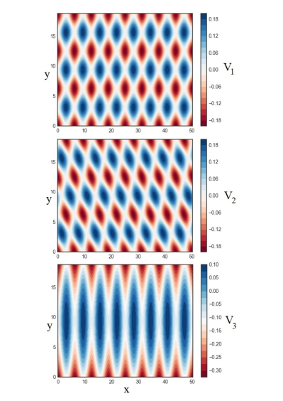
Figure 1: Three potentials shown by color for the three cases from (LABEL:eq:ham2) at $V=V_{1}$ (top panel), $V=V_{2}$ (middle panel), $V=V_{3}$ (bottom panel, here $K=0.1$, $K_{h}=0.005$).

As in zakharovprb the numerical simulations are based on the combination of Boost.odeint odeint and VexCL demidov2013 ; vexcl libraries and employ the approach described in ahnert2014 in order to accelerate the solution with NVIDIA CUDA technology. The equations (2) are solved by Verlet method, where each particle is handled by a single GPU thread. Since Coulomb interactions are decreasing with distance between particles, the interactions for the 2D case are cut off at the radius $R_{C}=6\ell=12\pi$, that allows to reduce the computational complexity of the algorithm from $O(N^{2})$ to $O(N\log N)$. In order to avoid close encounters between particles leading to numerical instability, the screening length $a=0.7$ is used. At such a value of $a$ the interaction energy is still significantly larger than the typical kinetic energies of particles ($T\ll 1/a$) and the screening does not significantly affect the interactions of particles. The source code is available at
https://gitlab.com/ddemidov/thermoelectric2d . The numerical simulations were run at OLYMPE CALMIP cluster olympe with NVIDIA Tesla V100 GPUs and partially at Kazan Federal University with NVIDIA Tesla C2070 GPUs.

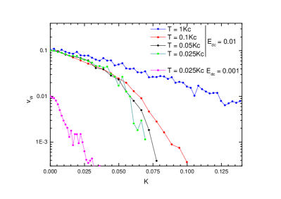
Figure 2: Dependence of the Wigner crystal (5 stripes) $v_{W}$ on the potential parameter $K$ for 2D system with $\nu=34/21$ at different values of driving force $E_{dc}$ and temperature $T$; here $K_{c}=0.0462$ is the critical potential amplitude for the Aubry transition in 1D case. The system has $L=21$ cells in $x$-axis and $L_{y}=5$ cells in $y$-axis and $N=34\times 5$ electrons; here the potential $V=V_{1}$ in (LABEL:eq:ham2).

In this work we consider only the problem of classical charges. Indeed, as shown in fki2007 the dimensionless Planck constant of the system is $\hbar_{\rm eff}=$ $\hbar/$ $(e\sqrt{m\ell/2\pi})$. For a typical lattice period $\ell\approx 1\rm\mu m$, $\nu\sim 1$ and electrons on a periodic potential of liquid helium we have a very small effective Planck constant $\hbar_{\rm eff}\approx 2\times 10^{-3}$.

3 Equilibrium positions of electrons

As for the 1D case the equilibrium static positions of electrons in a periodic potential are determined by the conditions $\partial H/\partial x_{i}=\partial H/\partial y_{i}=0$, $P_{ix}=P_{iy}=0$ fki2007 ; aubry . In the approximation of nearest neighbor interacting electrons, taking into account only nearby cells in $x$ and $y$ directions, this leads to the map for recurrent electron positions $x_{i},y_{j}$

$$p_{x,i+1}=p_{x,i}+Kg_{x}(x_{i})\;,\;\;x_{i+1}=x_{i}+F_{p_{x,i+1}}\;,$$

$$p_{y,j+1}=p_{y,j}+Kg_{y}(y_{j})\;,\;\;y_{j+1}=y_{j}+F_{p_{y,j+1}}\;,$$ (3)

where the effective momentum conjugated to $x_{i}$ and $y_{j}$, are $p_{x,i}=-dV/dx_{i}=(x_{i}-x_{i-1})/R^{3}$ and $p_{y,j}=-dV/dy_{j}=(y_{j}-y_{j-1})/R^{3}$ with $R^{2}=(x_{i}-x_{i-1})^{2}+(y_{j}-y_{j-1})^{2}+a^{2}$ and the kick functions $Kg_{x}(x_{i})=\left.-dV/dx\right|_{x=x_{i}}$ $=-K\sin x_{i}$ and $Kg_{y}(y_{j})=\left.-dV/dy\right|_{y=y_{j}}$ $=-K\sin y_{j}$ (for $V=V_{1}$). The functions $F_{p_{x,i+1}};F_{p_{y,j+1}}$ express the changes $x_{i+1}-x_{i};y_{j+1}-y_{j}$. For 1D case the recursive map for electron positions has an explicit symplectic form fki2007 ; lagesepjd ; zakharovprb (e.g. see Eq.(3) in lagesepjd ). This 1D map can be approximately reduced to the Chirikov standard map chirikov ; fki2007 ; lagesepjd that allows to obtain the analytical dependence for the Aubry transition on charge density. We note that if we neglect electron interactions between different stripes then we obtain approximately from (3) the 1D map studied in fki2007 ; lagesepjd ; zakharovprb .

However, interactions between stripes, represented by cells in $y$-axis, play an important role and hence in 2D case the map is much more complicated having an implicit form. Also from the dynamical view point it corresponds to the case of two times represented by indices $i$ and $j$. Such maps have been never studied from a mathematical view point that makes their analysis very complicated.

Due to these reasons we do not enter in the mathematical analysis of such maps. Instead, we directly study the transport properties on electrons described in next Sections.

4 Properties of electron current

In the frame of described Langevin approach we determine numerically the average flow velocity $v_{W}$ of the Wigner crystal in $x$-direction under the influence of a static electric field $E_{dc}$ using periodic boundary conditions in $x$-axis. In absence of periodic potential the crystal flows with the free electron velocity $v_{0}=E_{dc}/\eta$ (such a case was also discussed in zakharovprb ).

A typical dependence of $v_{W}$ on the potential amplitude $K$ at different values of temperature $T$ and static field $E_{dc}$ are shown in Figure 2 for the potential $V=V_{1}$ in (LABEL:eq:ham2). This data shows that at fixed $T$ the current velocity $v_{W}$ drops exponentially with increase of the potential amplitude $K$. This is consistent with the presence of Aubry transition from the Aubry pinned phase at $K>K_{c2}$ to the KAM sliding phase at $K<K_{c2}$. Here $K_{c2}$ is a certain critical amplitude of the transition. We can estimate that $K_{c2}\sim 0.02$ being approximately by a factor of 2 smaller comparing to the critical amplitude $K=K_{c}=0.0462$ in 1D at $\nu=1.618..$ fki2007 ; lagesepjd ; ztzs . At the same time an exact determination of $K_{c2}$ requires a detailed numerical analysis of transport at rather small $E_{dc}$ values and small temperatures. Indeed the comparisons of $v_{W}$ values at $E_{dc}=0.01$ and $0.001$ shows that at small $K$ values we have a linear regime with $v_{W}\sim E_{dc}/\eta$ but at $K\approx 0.02$ such a linear response starts to be destroyed pointing that $K_{c2}$ can be somewhat smaller with $K_{c2}\sim 0.015$. In fact, the situation in 2D case is more complicated compared to 1D case. Indeed, in 1D for $K>K_{c}$ there are no KAM curves and electrons should overcome a potential barrier to propagate along the lattice (while for $K<K_{c}$ they can freely slide along the lattice as it is guaranteed by the Aubry theorem aubry ). In 2D case the situation is more complex since even at large $K>K_{c2}$ there are formally straight paths propagating in $x$-direction, but it is possible that they are not really accessible due to interactions between electrons. Thus we estimate that in 2D lattice with $V=V_{1}$ in (LABEL:eq:ham2) we have at $\nu\approx 1.618$ the Aubry transition at $K_{c2}\approx 0.015-0.02$. The exact value of $K_{c2}$ is not very important for our further thermoelectric studies which are performed at $K$ values being significantly larger then $K_{c2}$ and at larger temperatures $T$.

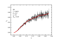
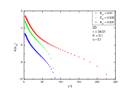
Figure 3: Left panel: dependence of Wigner crystal velocity $v_{W}$ on temperature $T$ at $K=0.1$, $L=21$, $L_{y}=5$, $N_{tot}=21\times 5$, $\nu=N_{tot}/LL_{y}=34/21$ and and driving force $E_{dc}=0.01$; data are smoothed by Savitzky-Golay filter with polynomial order 2 (points of window 150 in ORIGIN package) shown by red curve. Right panel: Thermal activation dependence of $ln(v_{W})$ on inverse temperature $1/T$ at parameters of left panel and different values of driving force $E_{dc}$, points show filtered data.

The thermoelectric propertied of the 2D system are studied for typical values $K\geq 0.1$ and $T\sim 0.1$. In such a regime a typical dependence of $v_{W}$ on $T$ is shown in Figure 3. The obtained $v_{W}$ values are characterized by a significant decrease of $v_{W}$ with decrease of $T$. The presence of fluctuations can be overcome by an averaging of data over Savitzky-Golay filter showing that on average the data are well described by the Arrhenius thermal activation dependence $\ln v_{W}=-B-A_{r}/T$ which works for a large temperature range $T>1/50$ (with $B=4.67$, $A_{R}=0.018$ at $E_{dc}=0.01$, $B=3.74$, $A_{R}=0.047$ at $E_{dc}=0.005$ and $B=5.25$, $A_{R}=0.044$ at $E_{dc}=0.001$). The fit parameters show that for such $E_{dc}$ values the current is described by the linear response dependence $v_{W}\propto E_{dc}$.

Above we discussed the square-lattice case with $V=V_{1}$ in (LABEL:eq:ham2). Similar results are obtained for two other lattices with $V=V_{2}$ and $V=V_{3}$. In the next Section we present the analysis of the thermoelectric properties in the linear response regime for these three lattice geometries.

We note that the self-diffusion of electrons in 2D periodic potential had been discussed recently in dykman but thermoelectricity and the Aubry pinned phase had not been analyzed there.

5 Seebeck coefficient

To compute the Seebeck coefficient of our system we use the procedure developed in ztzs . We use the Langevin description of a system evolution being a standard approach for analysis of the system when it has a fixed temperature created by the contact with the thermal bath or certain thermostat. The origins of this thermostat are not important since this description is universal politi . For the computation of the Seebeck coefficient $S$ we create a temperature gradient along $x$-direction. In the frame of the Langevin equation this is realized easily simply by imposing in (2) that $T$ is a function of an electron position along $x$-axis with $T=T(x)=T_{0}+Gx$. Here $T_{0}$ is the average temperature along the chain and $G=dT/dx$ is a small temperature gradient (here $x$ is a coordinate position of a given electron). For numerical computation of $S$ we have periodic conditions in $y$-axis and we introduce an elastic wall at $x=0$ keeping the Coulomb interactions of electrons through this wall (this makes density distribution homogeneous in absence of $E_{dc}$ and temperature gradient).

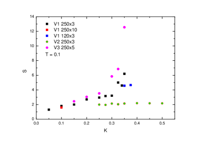
Figure 4: Dependence of Seebeck coefficient $S$ on $K$ for different periodic potentials given in (LABEL:eq:ham2) marked by $V_{1},V_{2},V_{3}$ with number of periodic cells $L_{x},L_{y}$ given; the total number of electrons being $N\approx 1.618L_{x}L_{y}$ and fixed temperature $T=0.1$ (here for $V=V_{3}$ case $K_{h}=0.002$).

At fixed temperature $T$ we apply a static field $E_{dc}$ which creates a voltage drop $\Delta V=2\pi LE_{dc}$ and a gradient of electron density $\nu(x)$ along the chain. Then at $E_{dc}=0$ within the Langevin equations (2) we impose a linear gradient of temperature $\Delta T$ along $x$-axis and in the stabilized steady-state regime determine the electron density gradient $g(\nu)=d\nu(x)/dx$ along $x$-direction. The data are obtained in the linear regime of relatively small $E_{dc}$ and $\Delta T$ values. Then the Seebeck coefficient is computed as $S=\Delta V/\Delta T$ where $\Delta V$ and $\Delta T$ are taken at such values that the density gradient from $\Delta V$ compensates those from $\Delta T$. Examples of such density gradients in presence of $E_{dc}$ and temperature gradient are shown in Appendix (Figures A.1,A.2,A.3,A.4).

The obtained dependencies of $S$ on temperature $T$ at different amplitudes $K$ of the periodic potential are shown in Fig. 4 for all three geometries of periodic potential given in (LABEL:eq:ham2). We discuss the dependence $S(K)$ for each geometry case.

For the square-lattice with $V=V_{1}$ in (LABEL:eq:ham2) we find a significant increase of $S$ with $K>K_{c2}$ at fixed temperature $T=0.1>K_{c2}$. At $K=0.1$ the values of $S$ are not affected by a variation of system size from $L_{y}=3$ up to $L_{y}=10$. At largest value of $K=0.35$ we obtain the largest value of $S=6.2$ at $L_{y}=3$. Unfortunately, at such large $K$ values very long simulation times are required to reach the steady-state in this strongly pinned Aubry phase. We expect that at larger transverse size $L_{y}$ longer times are required to reach the steady-state and our maximal simulation time $t=2\times 10^{6}$ is not sufficient for $L_{x}=250$ and $L_{y}>3$ for $K\approx 0.3$. A decrease of number of cells in $x$-axis down to $L_{x}=120$ at $L_{y}=3$ leads to a moderate reduction of $S$ down to $S=4.57$ from its value $S=6.2$ at $L_{x}=250$ at $K=0.35$. However, in this strongly pinned regime we have rather strong fluctuations of $S$ with small variations of $K$ and we attribute this variation with $L_{x}$ to fluctuations. We checked that an increase of $T$ from $0.1$ up to $0.3$ at $K=0.1$ ($L_{x}=250,L_{y}=3$) leads to a reduction of $S$ approximately by $20\%$. We checked that an increase of $T$ from $0.1$ up to $0.2$ at $K=0.3$ ($V_{3}$, $L_{x}=250,L_{y}=5$) leads to a reduction of $S$ approximately by $14\%$.

From a physical view point at large values $T\gg K$ the influence of periodic potential becomes small and we are getting moderate $S\sim 1$ values corresponding to the sliding KAM phase. A similar dependence of $S$ on temperature has been found for 1D case (e.g. see right panel of Fig.3 in fki2007 ).

The case of a diamond lattice with $V=V_{2}$ in (LABEL:eq:ham2) is also presented in Figure 4. In this case the dependence $S(K)$ is practically absent ($S$ is increased only by 10% when $K$ is increased from $0.25$ up to $0.5$). Thus the comparison of square and diamond lattices shows that the lattice geometry place a significant role. However, the reasons for significantly smaller $S$ values for the diamond lattice remain not rather clear. It is possible that for the diamond case there is a winding path that keeps the sliding of electrons in this case so that it is more close to the sliding KAM regime with moderate $S\sim 1$ values.

The strongest values up to $S\approx 12.5$ are found for the case $V=V_{3}$ for $K_{h}=0.002$ (see Figure 4). In this case the periodic potential is only in $x$-direction while in $y$-direction we have a harmonic potential. In a certain sense in this case there are no any free path for flying through the system at large values of $K$. Thus we assume that the pinned phase is more robust for such a geometry. We note that the results in Figure 4 are shown for $K_{h}=0.002$. At such a value of $K_{h}$ the harmonic potential is relatively weak and electrons still cover all $L_{y}=5$ cells in $y$-direction. As for the square lattice case we find that $S$ is decreasing with an increase of $T$ (see Figure A.5 of Appendix).

For $K=0.3$ we checked that an increase of $K_{h}$ from $K_{h}=0.001$ up to $K_{h}=0.008$ leads to a decrease of $S$ from $S=6.25$ down to $S=4.62$ (at fixed $T=0.1$ and $L_{x}=250,L_{y}=5$). We interpret this result assuming that at small $h$ values electrons have more flexibility in $y$-direction that leads to larger $S$ values. At $K_{h}=0.002$ we also checked that an increase of $L_{y}=5$ up to $L_{y}=11$ is sufficient to create a channel of electrons distributed in such a way that they do not touch the boundary in $y$-direction; however, in such a case we obtain $S=9.3$ (at $L_{y}=11$, $K_{h}=0.002$, $K=0.3$) being higher compared to the case presented in Figure 4 with $S=5.85$ at $L_{y}=5,K_{h}=0.002,K=0.3$. We explain this by the fact that for $L_{y}=11$ the effective electron density is decreased comparing to $L_{y}=5$ case (the total number of electorns is the same in both cases) and thus the electron interactions are effectively reduced that leads to a more pinned regime with a larger $S$ value.

The results discussed above are obtained for a fixed electron density $\nu\approx 1.618$, We checked that for $V=V_{3}$ case the value of $S$ is not significantly affected by an increase of $\nu$ up to $\nu=2.618$ where we obtained $S\approx 4$ at $K=0.3$, $L=250,L_{y}=5,K_{h}=0.006$. However, further more detailed investigation of dependence of $S$ on density $\nu$ are highly desirable.

The obtained results show that it is possible to have rather large Seebeck coefficients $S\approx 12\gg 1$ at certain lattice geometries in the Aubry pinned phase.

Of course, it would be very interesting to obtain the figure of merit $ZT$ for the above lattices. However, the computation of thermal conductivity $\kappa$, following the procedure described in ztzs ; lagesepjd , was not stabilized at maximal computational times $t=2\times 10^{6}$. We attribute this to long times required for phonon (plasmon) equilibrium to be reached in our 2D system with about 2000 electrons. Indeed, in 1D studies reported in ztzs ; lagesepjd much larger times had been used ($t\sim 10^{8}$) with smaller system sizes and about 50 - 100 electrons.

6 Discussion

In this work we presented numerical modeling of electron transport and themoelectricity in 2D periodic lattices of different geometries. We note that similar to 1D case discussed in ztzs ; lagesepjd there is a transition from sliding KAM phase at $K<K_{c2}$ to the Aubry pinned phase at $K>K_{c2}$ where the electron current drops exponentially with increase of $K$. However, compared to 1D case this transition is not so sharp probably due to presence of more complex pathways for sliding of electrons.

While the KAM phase has moderate values of Seebeck coefficient $S\sim 1$ the Aubry phase is characterized by a significant growth of $S$ with $K$ up to the highest value $S\approx 12$ found in our numerical simulations. At the same time it is established that a change of geometry can lead to a significant reduction of $S$ at the same amplitudes $K$ of periodic potential. We attribute such a feature to presence of free electron pathways crossing the whole system at certain geometries thus reducing maximal $S$ values.

The maximal value of $S\sim 12$ obtained in this study is still smaller than the extreme values of $S$ obtained in certain experiments. Thus in experiments with quasi-one-dimensional conductor $\rm(TMTSF)_{2}PF_{6}$ espci as high as $S=400k_{B}/e\approx 35mV/K$ value had been reached at low temperatures (see Fig. 3 in espci ). Rather high values of $S\approx 50k_{B}/e$ had been observed in highly resistive two-dimensional semiconductor (pinned) samples of micron size (see Fig. 8 in pepper ). The high values of $S\approx 30k_{B}/e$ have been reported recently for CoSbS single crystals kotliar .

In this studies we did not reach such high $S$ values but we obtain a clear dependence showing that $S$ is rapidly growing with increase of potential amplitude $K$ and that it is also growing with a decrease of temperature $T$. Unfortunately, very high $S$ values appear only inside the strongly pinned Aubry phase where the times of numerical simulations become very large to reach the steady-state regime. We are restricted by CPU time available for our numerical simulations and thus we were not able to penetrate inside such strongly pinned phase. But our results clearly show that even higher value $S\gg 10$ can be reached in the strong pinned regime.

We think that the proposed investigations of themoelectric properties of Wigner crystal in 2D periodic lattice are well accessible for experiments with low temperature electrons on a surface of liquid helium in the regimes similar to those discussed in kono1d ; konstantinov . Indeed, for a typical lattice period $\ell=1\mu m$ the potential amplitude $K=0.1$ corresponds to $V_{A}=Ke^{2}/(\ell/2pi)\approx 10K$ (Kelvin) that can be reached at rather weak potential modulation in space. Such $V_{A}$ can be significantly larger than electron temperature which easily takes values of $T=0.1K$. Thus we expect that such experiments will allow to obtain understanding of fundamental properties of thermoelectricity. As discussed in tosatti1 they can be also very useful for understanding of the fundamental aspects of friction at nanoscale.

7 Acknowledgments

We thank N. Beysengulov, A.D. Chepelianskii, J. Lages, D.A. Tayurskii and O.V. Zhirov for useful remarks and discussions.

This work was supported in part by the Programme Investissements d’Avenir ANR-11-IDEX-0002-02, reference ANR-10-LABX-0037-NEXT (project THETRACOM). This work was granted access to the HPC GPU resources of CALMIP (Toulouse) under the allocation 2019-P0110. The development of the VexCL library was partially funded by the state assignment to the Joint supercomputer center of the Russian Academy of sciences for scientific research. The work of M.Y. Zakharov was partially funded by the subsidy allocated to Kazan Federal University for the state assignment in the sphere of scientific activities (project $N^{\circ}$ 3.9779.2017/8.9).

8 Author contribution statement

All authors equally contributed to all stages of this work.

APPENDIX

A.1 Appendix

In Figures A.1,A.2,A.3,A.4 we show the variation of electron density induced by an external static field $E_{dc}$ and temperature gradient $dT/dx\propto\Delta T/T_{0}$ (here $T_{0}$ is the average sample temperature and $\Delta T$ is the temperature difference at the ends of the sample).

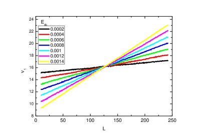
Figure A.1: Dependence of 1D electron density (averaged over $y$-axis) on $x=L$ coordinate at different values of applied static field $E_{dc}$. Here $V=V_{1}$ in (LABEL:eq:ham2), $K=0.1,T_{0}=0.1$, the system has $LL_{y}=250\times 10$ period cells with average density of electrons per cell being $\nu\approx 1.618$ (in total $N_{tot}=4045$ electrons); the physical time is $t=2\times 10^{6}$.

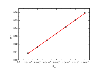
Figure A.2: Dependence of the gradient of electron density $g(\nu_{1})$ on static field $E_{dc}$ for parameters of Figure A.1; $\nu=\nu_{1}=1.618$.

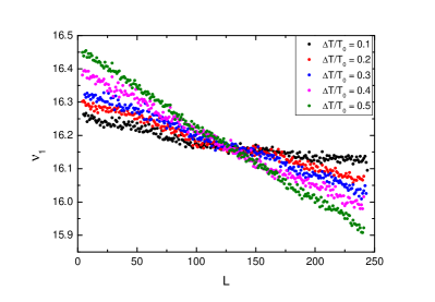
Figure A.3: Dependence of 1D electron density (averaged over $y$-axis) on $x=L$ coordinate at different values of temperature difference $\Delta T$ at the end of the sample; other parameters are as in Figure A.1, $E_{dc}=0$.

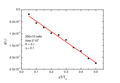
Figure A.4: Dependence of the gradient of electron density $g(\nu_{1})$ on temperature difference $\Delta T$ at the end of the sample; other parameters are as in Figure A.1, $E_{dc}=0$.

Figure A.5 shows the dependence $S(K)$ for the harmonic channel at different temperature and system size values.

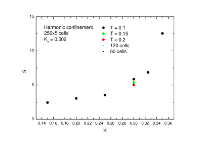
Figure A.5: Dependence of Seebeck coefficient $S$ on $K$ the system with harmonic confinement $V=V_{3}$ in (LABEL:eq:ham2) at $K_{h}=0.002$ for $L=250,L_{y}=5$ and $T=0.1$ (black points), $T=0.15$ (green point), $T=0.2$ (red point); cyan and blue points show data at $T=0.1$ for $L=120,L_{y}=5$ and $L=60,L_{y}=5$ respectively. .

References

- (1) E. Wigner, On the interaction of electrons in metals, Phys. Rev. 46, 1002 (1934).
- (2) Y. Monarkha and K. Kono, Two-Ddmensional Coulomb liquids and solids, Springer-Verlag, Berlin (2004).
- (3) J.S. Meyer and K.A. Matveev, Wigner crystal physics in quantum wires, J. Phys. C.: Condens. Mat. 21, 023203 (2009).
- (4) I. Garcia-Mata, O.V. Zhirov, and D.L. Shepelyansky, Frenkel-Kontorova model with cold trapped ions, Eur. Phys. J. D 41, 325 (2007).
- (5) O.M. Braun and Yu.S. Kivshar, The Frenkel-Kontorova Model: Concepts, Methods, Applications, Springer-Verlag, Berlin (2004).
- (6) B. V. Chirikov, A universal instability of many-dimensional oscillator systems , Phys. Rep. 52 (1979) 263.
- (7) A.J.Lichtenberg, M.A.Lieberman, Regular and chaotic dynamics, Springer, Berlin (1992).
- (8) J.D. Meiss, Symplectic maps, variational principles, and transport, Rev. Mod. Phys. 64(3), 795 (1992).
- (9) B. Chirikov and D. Shepelyansky, Chirikov standard map, Scholarpedia 3(3), 3550 (2008).
- (10) S. Aubry, The twist map, the extended Frenkel-Kontorova model and the devil’s staircase, Physica D 7 (1983) 240.
- (11) O.V. Zhirov, and D.L. Shepelyansky, Thermoelectricity of Wigner crystal in a periodic potential, Europhys. Lett. 103, 68008 (2013).
- (12) O.V.Zhirov, J.Lages and D.L.Shepelyansky, Thermoelectricity of cold ions in optical lattices, Eur. Phys. J. D 73, 149 (2019).
- (13) A.F. Ioffe, Semiconductor thermoelements, and thermoelectric cooling, Infosearch, Ltd (1957).
- (14) A.F. Ioffe and L.S. Stil’bans, Physical problems of thermoelectricity, Rep. Prog. Phys. 22, 167 (1959).
- (15) A. Majumdar, Thermoelectricity in semiconductor nanostructures, Science 303, 777 (2004).
- (16) H.J. Goldsmid, Introduction to thermoelectricity, Springer, Berlin (2009).
- (17) N. Li, J. Ren, L. Wang, G. Zhang, P. Hanggi, and B. Li, Phononics: manipulating heat flow with electronic analogs and beyond, Rev. Mod. Phys. 84, 1045 (2012).
- (18) B.G. Levi, Simple compound manifests record-high thermoelectric performance, Phys. Tod. 67(6), 14 (2014).
- (19) J. He, and T.M. Tritt, Advances in thermoelectric materials research: looking back and moving forward, Science 357, eaak9997 (2017).
- (20) J.P. Heremans, M.S. Dresselhaus, L.E. Bell and D.T. Morelli, When thermoelectrics reached the nanoscale, Nature Nanotech. 8, 471 (2013).
- (21) D.G.-Rees, S.-S. Yeh, B.-C. Lee, K. Kono, and J.-J.Lin, Bistable transport properties of a quasi-one-dimensional Wigner solid on liquid helium under continuous driving, Phys. Rev. B 96, 205438 (2017).
- (22) J.-Y. Lin, A.V. Smorodin, A.O. Badrutdinov, and D. Konstantinov, Transport properties of a quasi-1D Wigner solid on liquid helium confined in a microchannel with periodic potential, J. Low Temp. Phys. 195, 289 (2019).
- (23) T. Pruttivarasin, M. Ramm, I. Talukdar, A. Kreuter, and H. Haffner, Trapped ions in optical lattices for probing oscillator chain models, New J. Phys. 13, 075012 (2011).
- (24) A. Bylinskii, D. Gangloff, and V. Vuletic, Tuning friction atom-by-atom in an ion-crystal simulator, Science 348, 1115 (2015).
- (25) A. Bylinskii, D. Gangloff, I. Countis, and V. Vuletic, Observation of Aubry-type transition in finite atom chains via friction, Nature Mat. 11, 717 (2016).
- (26) J.Kiethe, R. Nigmatullin, D. Kalincev, T. Schmirander, and T.E. Mehlstaubler, Probing nanofriction and Aubry-type signatures in a finite self-organized system, Nature Comm. 8 15364 (2017).
- (27) T. Laupretre, R.B. Linnet, I.D. Leroux, H. Landa, A. Dantan, and M. Drewsen, Controlling the potential landscape and normal modes of ion Coulomb crystals by a standing-wave optical potential, Phys. Rev. A 99, 031401(R) (2019).
- (28) T. Brazda, A. Silva, N. Manini, A. Vanossi, R. Guerra, E. Tosatti, and C. Bechinger, Experimental observation of the Aubry transition in two-dimensional colloidal monolayers, Phys. Rev. X 8, 011050 (2018).
- (29) M.Y.Zakharov, D.Demidov and D.L.Shepelyansky, transport properties of a Wigner crystal in one- and two-dimensional asymmetric periodic potentials: Wigner crystal diode, Phys. Rev. B 99, 155416 (2019).
- (30) S. Lepri, R. Livi, and A. Politi, Thermal conduction in classical low-dimensional lattices, Phys. Rep. 377, 1 (2003).
- (31) K. Ahnert and M. Mulansky, Odeint — solving ordinary differential equations in C++, In IP Conf. Proc., 1389, 1586 (2011).
- (32) D. Demidov, K. Ahnert, K. Rupp, and P. Gottschling, Programming CUDA and OpenCL: A case study using modern C++ Libraries. SIAM J. Sci. Comput. 35(5), C453 (2013).
- (33) D. Demidov, VEXCL, https://github.com/ddemidov/vexcl. Accessed Oct (2019).
- (34) K. Ahnert, D. Demidov, and M. Mulansky, Solving ordinary differential equations on GPUs, In Volodymyr Kindratenko, Editor, Numerical Computations with GPUs, pages 125–157, Springer, Berlin (2014).
- (35) Olympe, CALMIP https://www.calmip.univ-toulouse.fr/spip.php?article582. Accessed Oct (2019).
- (36) K. Moskovtsev, and M.I. Dykman, Self-diffusion in a spatially modulated system of electrons on helium, J. Low Temp. Phys. 195, 266 (2019).
- (37) Y. Machida, X. Lin, W. Kang, K. Izawa and K. Behnia, Colossal Seebeck Coefficient of Hopping Electrons in , Phys. Rev. Lett. 116, 087003 (2016).
- (38) V. Narayan, M. Pepper, J. Griffiths, H. Beere, F. Sfigakis, G. Jones, D. Ritchie and A. Ghosh, Unconventional metallicity and giant thermopower in a strongly interacting two-dimensional electron system, Phys. Rev. B 86, 125406 (2012).
- (39) Q. Du, M. Abeykoon, Y.Liu, G. Kotliar and C. Petrovic, Low-temperature thermopower in CoSbS, Phys. Rev. Lett. 123, 076602 (2019).
- (40) A. Benassi, A. Vanossi, and E. Tosatti, Nanofriction in cold ion traps, Nature Comm. 2, 236 (2011).