Multi-Resolution Overlapping Stripes Network for Person Re-Identification

Abstract

This paper addresses the person re-identification (PReID) problem by combining global and local information at multiple feature resolutions with different loss functions. Many previous studies address this problem using either part-based features or global features. In case of part-based representation, the spatial correlation between these parts is not considered, while global-based representation are not sensitive to spatial variations. This paper presents a part-based model with a multi-resolution network that uses different level of features. The output of the last two conv blocks is then partitioned horizontally and processed in pairs with overlapping stripes to cover the important information that might lie between parts. We use different loss functions to combine local and global information for classification. Experimental results on a benchmark dataset demonstrate that the presented method outperforms the state-of-the-art methods.

Index Terms—  Person re-identification, classification, CNN, multi-resolution.

1 Introduction

Person re-identification (PReID) is the task of identifying the presence of a person from multiple surveillance cameras. Given a query image, the aim is to retrieve all images of the specified person in a gallery dataset. This task has attracted the attention of many researchers in computer vision for its great importance in multiple applications such as video surveillance for public security. With the recent success of deep convolution neural networks (CNNs), PReID performance has made significant progress. Deep representations provide high discriminative ability, especially when aggregated from part-based deep local features.

Current related studies in PReID can be categorized to global feature-based and local part-based models. The local part-based models perform better with certain variations such as partial occlusion. Sun et al.[1], for instance, presented the part-based convolutional baseline (PCB) that horizontally divided the last feature maps into multiple stripes where each one contains part of the person’s body in the input image. After that, a refinement mechanism was applied to each piece to guarantee that the feature map of this part focuses on the correct body part. PCB is a simple and effective framework that outperforms the other part-based models. However, it does not consider global features which play an important role in recognition and identification tasks and are normally robust to multiple variations. On the other hand, since their stripes have no overlaps, it loses important information that might lie at the edges of the divided stripes.

Global feature-based models focus on contour, shape, and texture representations. For example, Wang et al.[2] built the DaReNet model based only on global information using a multiple granularity network to extract global features at different resolutions. Hermans et al.[3] presented a ResNet-50 based classifier which uses global information. Shen et al.[4] combined global features with random walk algorithm. Li et al.[5] proposed an attention-based model. Luo et al.[6] reported a strong CNN based model with bag of learning tricks including augmentation and regularization. However, those methods may fail in the presence of object occlusion, multiple poses and lighting variations and usually depend on pre- and post-processing steps to boost their performances.

To address the above problems, other groups combined both global and local features. Li et al.[7] fused local and global features while using mutual learning but they did not train the model with multiple loss functions. While He et al.[8] used attention aware model that combines global and local features. Quan et al.[9] introduced neural architecture search to PReID by focusing on searching the best CNN structure and applied the part-aware module in PReID search space that employs both part and global information.

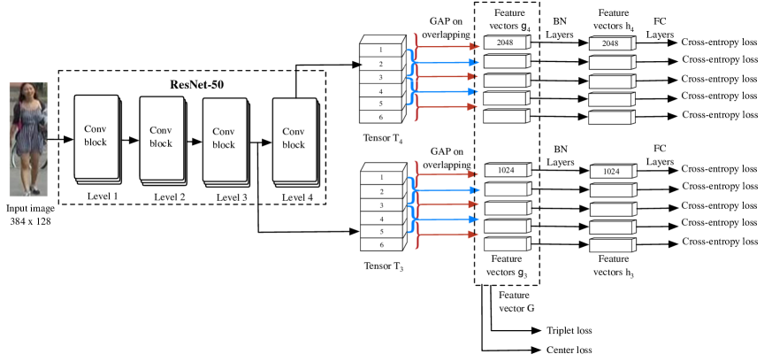
Fig. 1: Illustration of multi-resolution overlapping stripes (MROS) model for PReID. The backbone network is ResNet-50 [10] with four conv blocks. The input image goes through ResNet-50 to generate two feature tensors T_j where $j=3$ or $4$, which are used by the overlapping stripe approach to obtain ${\bm{g}}_{j}$ vectors. The global feature vector ${\bm{G}}$ is then obtained by as a concatenation of ${\bm{g}}_{j}$ while the local feature vectors ${\bm{h}}_{j}$ are obtained by applying a BN layer after ${\bm{g}}_{j}$ Triplet and center losses are finally applied to ${\bm{G}}$ and cross-entropy loss applied to ${\bm{h}}_{j}$. The model trained with loss $L=L_{triplet}+\beta L_{center}+L_{cross}$.

Different loss functions have also been presented to boost the performance of the PReID models. Two loss functions are widely used: triplet loss [11] and cross-entropy loss [12]. Triplet loss is based on the feature metrics distances while cross-entropy loss is based on classification with fully connected (FC) layers. Hermans et al.[3] and Zhang et al.[13] modified triplet loss to increase the training performance. Fan et al.[14] presented a classification model based on an extended version of the cross-entropy loss function and a warming-up learning rate to learn a hypersphere manifold embedding. Recently, several models [8, 9] are trained using a combination of triplet loss and cross-entropy loss.

In this paper, we propose a multi-resolution overlapping stripes (MROS) model by combining global and local information at multiple resolutions with different loss functions. First, based on the residual network (ResNet50) [10], multiple levels are created each of which has different resolution. Inspired by the PCB model [1], the feature map from each level is divided horizontally into multi-stripes which will be processed later in pairs with overlapping rather than individually. The overlapping avoids lost of information at the boundaries/edges of stripes which usually occurs when using the part-based models. Secondly, instead of using the features from all multi-resolution levels for classification as in [2], only the features from the last two levels are considered. This is because the later levels of the model learn more semantic representations compared to the early layers. Thirdly, local and global features are combined using different loss functions. Experiments on the Market-1501 [15] dataset – a large-scale person dataset most widely used for the PReID task – show the effectiveness of the presented approach.

2 Multi-Resolution Overlapping Stripes Model

Given a collection of images divided into query, gallery and training sets, PReID aims to find the images of each pedestrian from a query set in the gallery set. To address this problem, we propose a multi-resolution overlapping stripes (MROS) model as shown in Fig. 1.

The MROS model is constructed as follows. Firstly, inspired by the model presented in DaReNet [2], we construct multi-level features model. Instead of using every feature level, we only use the last two feature levels (Section 2.1). This reduces the computational complexity and increases the model performance. Secondly, the local features are extracted by extending the PCB [1] network. Instead of using $s$ stationary and non-overlapping stripes, an overlapping partitioning technique is employed based on pairs of stripes rather than individual ones (Section 2.1). This technique helps our method to avoid missing features at the boundaries of the individual stripes. Lastly, inspired by the recent successful performances achieved by local and global feature fusion [5, 7, 8] and loss function fusion [6, 8, 9], various loss functions based on local and global features are employed in this work to boost the performance of the model (Section 2.2).

2.1 Network Architecture

As shown in Figure 1, the backbone network for our model is the ResNet-50. It is a CNN trained on more than a million images from the ImageNet [16] database and consists of four convolutional blocks $T_{i}$, where $i=\left\{1,\ldots,4\right\}$. To build a multi-resolution model, we only consider the output of the last two conv blocks, i.e.tensors $T_{3}$ and $T_{4}$. The part-based model is constructed by dividing feature tensors $T_{3}$ and $T_{4}$ to $s=6$ equal stripes, then the adjacent stripes are grouped in pairs and the global average pooling (GAP) is applied on overlapping stripes. For each tensor $T_{j}$ with $j=3$ or $4$, the GAP operation generates new feature vectors ${\bm{g}}_{j}$ with $s-1$, $5$, stripes in each. After that, batch normalization (BN) layers are applied on ${\bm{g}}_{j}$ to obtain ${\bm{h}}_{j}$ to overcome the overfitting and boost the performance of the system.

For classification, FC layers are added after the local features ${\bm{h}}_{j}$. Note that FC layers for ${\bm{h}}_{4}$ are 2048-dimensional while FC layers for ${\bm{h}}_{3}$ are 1024-dimensional. Feature descriptor ${\bm{G}}$ is defined by concatenating the feature vectors ${\bm{g}}_{j}$. Feature vectors ${\bm{G}}$ and ${\bm{h}}_{j}$ are used during the training while feature vector ${\bm{G}}$ is used at testing.

2.2 Loss Functions

During the training, the MROS model is optimized by minimizing the fusion of three different loss functions including the triplet loss combined with center loss for metric learning and the cross-entropy loss for classification.

Firstly, instead of calculating individual losses for each stripe, a global feature ${\bm{G}}$ is defined by concatenating feature vectors ${\bm{g}}_{3}$ and ${\bm{g}}_{4}$. The batch-hard triplet loss [3] is then applied on the feature vector ${\bm{G}}$ as follows:

$$L_{triplet}=\sum_{i=1}^{P}\sum_{a=1}^{K}[\alpha+ \max\limits_{p=1..K}\|{\bm{G}}_{a}^{i}-{\bm{G}}_{p}^{i}\|_{2}$$ (1)

$$- \min_{\begin{subarray}{c}j=1..K\\ n=1..K\\ i\neq j\end{subarray}}\|{\bm{G}}_{a}^{i}-{\bm{G}}_{n}^{j}\|_{2}]_{+}$$

where $P$ is the number of identities in a batch, $K$ is the number of images for the same identities in a batch, $\alpha$ is loss margin, ${\bm{G}}_{a}$, ${\bm{G}}_{p}$ and ${\bm{G}}_{n}$ are features vectors from anchor, positive and negative samples.

At this stage, the center loss [12] is also applied on global feature vector ${\bm{G}}$ to minimize the feature distribution in the feature space as following:

$$L_{center}=\dfrac{1}{2}\sum_{i=1}^{m}\|{\bm{G}}^{i}-c_{y_{i}}\|_{2}^{2}$$ (2)

where $m$ is the batch size, $c_{y_{i}}$ is ${y_{i}}$th class center vector for the features.

Secondly, the cross-entropy loss is computed for each stripe of the local feature vectors ${\bm{h}}_{j}$ as follows:

$$L_{cross}=\sum_{i=1}^{m}log\dfrac{e^{W_{y_{i}}^{T}{\bm{h}}^{i}_{j}+b_{y_{i}}}}{\sum\limits_{c=1}^{C}e^{W_{c}^{T}{\bm{h}}^{i}_{j}+b_{c}}}$$ (3)

where $m$ is the batch size, $C$ is the number classes in the training set, $W$ is the weight vector for the FC layers and $b$ is the bias. Also, total cross-entropy loss is calculated as mean of all cross-entropy losses as follows:

$$L_{cross}^{{}^{\prime}}=\dfrac{1}{2*(s-1)}\sum\limits_{j=3}^{4}\sum\limits_{l=1}^{s-1}L_{cross}^{j,l}$$ (4)

The label smoothing (LS) [17] technique is applied to improve the accuracy and prevent classification overfitting.

Finally, the total loss function is calculated by the weighted sum of the previous losses in Equations 1, 2 and 4, where the priority of triplet loss and cross-entropy loss are kept equal.

$$\begin{split}L=L_{triplet}+\beta L_{center}+L_{cross}^{{}^{\prime}}\end{split}$$ (5)

where $\beta$ is the weight of center loss.

3 Experiments

The MROS is evaluated using the Market-1501 [15], which is a large-scale person dataset most widely used for PReID. It is collected from six different cameras with overlapping fields of view where five cameras have $1280\times 1080$ HD resolution and one camera has $720\times 576$ SD resolution. The dataset has $32,668$ bounding boxes generated using a person detector for $1,501$ individuals. Following [15], the dataset is split into $12,936$ images for training and $19,732$ images for testing. Single-query mode is used for searching the query images in gallery set individually.

The mean average precision (mAP) [15], Rank-1, Rank-5 and Rank-10 accuracies are used to evaluate the MROS performance. The area under the Precision-Recall curve also known as average precision (AP) is calculated for each query image. The mean value of APs over all queries is then calculated as mAP.

3.1 Experimental Setup

We use two Nvidia GeForce GTX $1080$ Ti GPUs with $3584$ CUDA cores and $11$ GB video memory for implementation. All implementations are done on Python $3.5$ with PyTorch [18] library.

Data augmentation is used to overcome the overfitting by artificially enlarging the training samples with class-preserving transformations. This helps to produce more training data and reduce overfitting. In our experiment, different types of data augmentation are employed including zero padding with $10$ pixels, random cropping, horizontal flipping with $0.5$ probability and image normalization with the same mean and standard deviation values as ImageNet dataset [16]. Random erasing [19] is also applied with $0.5$ probability and ImageNet pixel mean values.

We use the Adam method [20] as our optimizer using the warm-up learning rate technique [14] with $0.01$ coefficient and $10$ period epochs. The learning rate is set to $0.001$ and is reduced using the staircase function by a factor of $0.1$ after every $30$ epochs. The batch size is $128$ while $P$ and $K$ in Equation 1 are set to $32$ and $4$, respectively. The weight of center loss $\beta$ in Equation 5 is set to $0.0005$. The ECN [21] is used as re-ranking method.

3.2 Experimental Results

This section presents the performance evaluation of different settings of the MROS model on Market-1501 dataset. It also includes comparisons with the state-of-the-art methods.

To evaluate the effectiveness of each step of the presented model, we incrementally measure the accuracy as follows.

• Setting I presents the baseline model constructed using part-based features followed by none-overlapping stripes method with $s=6$ stripes to generate local feature vectors ${\bm{g}}_{4}$ and ${\bm{h}}_{4}$. During this experiment, all loss functions – triplet, center, and cross-entropy losses – are applied on local feature vectors ${\bm{g}}_{4}$ and ${\bm{h}}_{4}$.

• Setting II is similar to Setting I except that it uses overlapping stripes.

• Setting III evaluates the effectiveness of combining global and local features by generating the global feature vector ${\bm{G}}$ and using it with the triplet and center losses while using cross-entropy loss with ${\bm{h}}_{j}$.

• Setting IV evaluates the effectiveness of the multi-level features by considering last two level features, i.e.${\bm{g}}_{3}$ and ${\bm{g}}_{4}$.

#	MROS Settings	mAP	Rank-1
I	$s$ Non-Overlapping Stripes	81.8	93.2
II	$s-1$ Overlapping Stripes (OS)	82.8	93.5
III	OS with Global Features, ${\bm{G}}$	84.0	94.2
IV	Complete MROS	84.2	94.4

Table 1: Comparison of proposed three approaches on Market-1501 [15] dataset.

Table 1 presents these settings along with experimental results. The baseline Setting I achieves promising results, however, Setting II increases the performance by using overlapping stripes. On the other hand, using global and local features boosts the performance in Setting III. Finally, the best results are obtained by Setting IV which combines all previous settings with multi-resolution features.

Model	mAP	Rank-1	Rank-5	Rank-10
DaRe [2]	76.0	89.0	-	-
HA-CNN [5]	75.7	91.2	-	-
PCB [1]	77.4	92.3	97.2	98.2
TBN+ [7]	83.0	93.2	-	-
PCB+RPP [1]	81.6	93.8	97.5	98.5
MFBN [8]	84.9	93.9	-	-
SphereReID [14]	83.6	94.4	98.0	98.7
Auto-ReID [9]	85.1	94.5	98.5	99.0
Strong ReID [6]	85.9	94.5	-	-
Proposed MROS	84.2	94.4	97.8	98.7

Table 2: Comparison with the state-of-the-art results on the Market-1501 [15] dataset without re-ranking.

A comparison of the experimental results between MROS using single-query mode and the related methods are presented in Table 2 and Table 3 without and with re-ranking, respectively. The MROS model achieved mAP = 84.2% and Rank-1 = 94.4% without re-ranking and mAP = 93.5% and Rank-1 = 95.5% with re-ranking [21]. The results in Table 2 show that the proposed MROS model without re-ranking achieves competitive performances. On the other hand, most of the re-ranked PReID models in Table 3 reported rank-1 results in a small margin $[95.1$-$95.4]$. As can be observed from the table, our MROS model outperforms the state-of-the-art models. This is because MROS is more able to learn body parts and the spatial correlation between them by employing the overlapping stripes and learn discriminative features by employing multi-resolution and different loss functions.

Model	mAP	Rank-1	Rank-5	Rank-10
DaRe [2]	86.7	89.0	-	-
GSRW [4]	82.5	92.7	96.9	98.1
PCB+RPP [1]	81.9	95.1	-	-
MFBN [8]	93.2	95.2	-	-
TBN+ [7]	91.3	95.4	-	-
Auto-ReID [9]	94.2	95.4	97.9	98.5
Strong ReID [6]	94.2	95.4	-	-
Proposed MROS	93.5	95.5	97.2	97.8

Table 3: Comparison with the state-of-the-art results on the Market-1501 [15] dataset with re-ranking.

4 Conclusions

This paper extended the part-based convolutional baseline (PCB) and the multi-resolution model to solve the problem of pedestrian retrieval. Using the residual network (ResNet50) as backbone network, multi-levels with different resolutions are created to generate feature maps. After that a simple uniform partition technique is applied on the last two conv blocks and the generated features are combined with overlapping. Using different types of loss functions, both global and local representations were considered for classification. Experimental results show that our approach outperforms the state-of-the-art methods.

References

- [1] Yifan Sun, Liang Zheng, Yi Yang, Qi Tian, and Shengjin Wang, “Beyond part models: Person retrieval with refined part pooling (and a strong convolutional baseline),” in Computer Vision – ECCV, Vittorio Ferrari, Martial Hebert, Cristian Sminchisescu, and Yair Weiss, Eds. 2018, pp. 501–518, Springer International Publishing.
- [2] Y. Wang, L. Wang, Y. You, X. Zou, V. Chen, S. Li, G. Huang, B. Hariharan, and K. Q. Weinberger, “Resource aware person re-identification across multiple resolutions,” in The IEEE/CVF Conference on Computer Vision and Pattern Recognition, 2018, pp. 8042–8051.
- [3] Alexander Hermans, Lucas Beyer, and Bastian Leibe, “In defense of the triplet loss for person re-identification,” ArXiv, vol. abs/1703.07737, 2017.
- [4] Yantao Shen, Hongsheng Li, Tong Xiao, Shuai Yi, Dapeng Chen, and Xiaogang Wang, “Deep group-shuffling random walk for person re-identification,” in Proceedings of the IEEE Conference on Computer Vision and Pattern Recognition, 2018, pp. 2265–2274.
- [5] W. Li, X. Zhu, and S. Gong, “Harmonious attention network for person re-identification,” in The IEEE/CVF Conference on Computer Vision and Pattern Recognition, 2018, pp. 2285–2294.
- [6] Hao Luo, Youzhi Gu, Xingyu Liao, Shenqi Lai, and Wei Jiang, “Bag of tricks and a strong baseline for deep person re-identification,” in The IEEE Conference on Computer Vision and Pattern Recognition (CVPR) Workshops, 2019.
- [7] Hui Li, Meng Yang, Zhihui Lai, Weishi Zheng, and Zitong Yu, “Pedestrian re-identification based on tree branch network with local and global learning,” arXiv preprint arXiv:1904.00355, 2019.
- [8] Shengyi He, Junmin Wu, and Yuqian Li, “Mfbn: An efficient base model for person re-identification,” in Proceedings of the 2019 4th International Conference on Mathematics and Artificial Intelligence. ACM, 2019, pp. 44–50.
- [9] Ruijie Quan, Xuanyi Dong, Yuehua Wu, Linchao Zhu, and Yi Yang, “Auto-reid: Searching for a part-aware convnet for person re-identification,” ArXiv, vol. abs/1903.09776, 2019.
- [10] K. He, X. Zhang, S. Ren, and J. Sun, “Deep residual learning for image recognition,” in The IEEE Conference on Computer Vision and Pattern Recognition (CVPR), 2016, pp. 770–778.
- [11] Florian Schroff, Dmitry Kalenichenko, and James Philbin, “Facenet: A unified embedding for face recognition and clustering,” in The IEEE Conference on Computer Vision and Pattern Recognition–CVPR, 2015, pp. 815–823.
- [12] Yandong Wen, Kaipeng Zhang, Zhifeng Li, and Yu Qiao, “A discriminative feature learning approach for deep face recognition,” in European conference on computer vision. Springer, 2016, pp. 499–515.
- [13] Yingying Zhang, Qiaoyong Zhong, Liang Ma, Di Xie, and Shiliang Pu, “Learning incremental triplet margin for person re-identification,” in Proceedings of the AAAI Conference on Artificial Intelligence, 2019, vol. 33, pp. 9243–9250.
- [14] Xing Fan, Wei Jiang, Hao Luo, and Mengjuan Fei, “Spherereid: Deep hypersphere manifold embedding for person re-identification,” Journal of Visual Communication and Image Representation, vol. 60, pp. 51 – 58, 2019.
- [15] Liang Zheng, Liyue Shen, Lu Tian, Shengjin Wang, Jingdong Wang, and Qi Tian, “Scalable person re-identification: A benchmark,” in Proceedings of the IEEE international conference on computer vision, 2015, pp. 1116–1124.
- [16] J. Deng, W. Dong, R. Socher, L.-J. Li, K. Li, and L. Fei-Fei, “ImageNet: A Large-Scale Hierarchical Image Database,” in CVPR09, 2009.
- [17] Christian Szegedy, Vincent Vanhoucke, Sergey Ioffe, Jonathon Shlens, and Zbigniew Wojna, “Rethinking the inception architecture for computer vision,” The IEEE Conference on Computer Vision and Pattern Recognition (CVPR), pp. 2818–2826, 2015.
- [18] Adam Paszke, Sam Gross, Soumith Chintala, Gregory Chanan, Edward Yang, Zachary DeVito, Zeming Lin, Alban Desmaison, Luca Antiga, and Adam Lerer, “Automatic differentiation in PyTorch,” in NIPS Autodiff Workshop, 2017.
- [19] Zhun Zhong, Liang Zheng, Guoliang Kang, Shaozi Li, and Yi Yang, “Random erasing data augmentation,” ArXiv, vol. abs/1708.04896, 2017.
- [20] Diederik P. Kingma and Jimmy Ba, “Adam: A method for stochastic optimization,” CoRR, vol. 1412.6980, 2014.
- [21] M Saquib Sarfraz, Arne Schumann, Andreas Eberle, and Rainer Stiefelhagen, “A pose-sensitive embedding for person re-identification with expanded cross neighborhood re-ranking,” in Proceedings of the IEEE Conference on Computer Vision and Pattern Recognition, 2018, pp. 420–429.