Kernel Stein Tests for Multiple Model Comparison

Abstract

We address the problem of non-parametric multiple model comparison: given $l$ candidate models, decide whether each candidate is as good as the best one(s) or worse than it. We propose two statistical tests, each controlling a different notion of decision errors. The first test, building on the post selection inference framework, provably controls the number of best models that are wrongly declared worse (false positive rate). The second test is based on multiple correction, and controls the proportion of the models declared worse but are in fact as good as the best (false discovery rate). We prove that under appropriate conditions the first test can yield a higher true positive rate than the second. Experimental results on toy and real (CelebA, Chicago Crime data) problems show that the two tests have high true positive rates with well-controlled error rates. By contrast, the naive approach of choosing the model with the lowest score without correction leads to more false positives.

1 Introduction

Given a sample (a set of i.i.d. observations), and a set of $l$ candidate models $\mathcal{M}$, we address the problem of non-parametric comparison of the relative fit of these candidate models. The comparison is non-parametric in the sense that the class of allowed candidate models is broad (mild assumptions on the models). All the given candidate models may be wrong; that is, the true data generating distribution may not be present in the candidate list. A widely used approach is to pre-select a divergence measure which computes a distance between a model and the sample (e.g., Fréchet Inception Distance (FID, [16]), Kernel Inception Distance [3] or others), and choose the model which gives the lowest estimate of the divergence. An issue with this approach is that multiple equally good models may give roughly the same estimate of the divergence, giving a wrong conclusion of the best model due to noise from the sample (see Table 1 in [17] for an example of a misleading conclusion resulted from direct comparison of two FID estimates).

It was this issue that motivates the development of a non-parametric hypothesis test of relative fit (RelMMD) between two candidate models [4]. The test uses as its test statistic the difference of two estimates of Maximum Mean Discrepancy (MMD, [14]), each measuring the distance between the generated sample from each model and the observed sample. It is known that if the kernel function used is characteristic [27, 11], the population MMD defines a metric on a large class of distributions. As a result, the magnitude of the relative test statistic provides a measure of relative fit, allowing one to decide a (significantly) better model when the statistic is sufficiently large. The key to avoiding the previously mentioned issue of false detection is to appropriately choose the threshold based on the null distribution, i.e., the distribution of the statistic when the two models are equally good. An extension of RelMMD to a linear-time relative test was considered by Jitkrittum et al. [17].

A limitation of the relative tests of RelMMD and others [4, 17] is that they are limited to the comparison of only $l=2$ candidate models. Indeed, taking the difference is inherently a function of two quantities, and it is unclear how the previous relative tests can be applied when there are $l>2$ candidate models. We note that relative fit testing is different from goodness-of-fit testing, which aims to decide whether a given model is the true distribution of a set of observations. The latter task may be achieved with the Kernel Stein Discrepancy (KSD) test [6, 23, 13] where, in the continuous case, the model is specified as a probability density function and needs only be known up to the normalizer. A discrete analogue of the KSD test is studied in [32]. When the model is represented by its sample, goodness-of-fit testing reduces to two-sample testing, and may be carried out with the MMD test [14], its incomplete U-statistic variants [33, 31], the ME and SCF tests [7, 18], and related kernel-based tests [8, 10], among others. To reiterate, we stress that in general multiple model comparison differs from multiple goodness-of-fit tests. While the latter may be addressed with $l$ individual goodness-of-fit tests (one for each candidate), the former requires comparing $l$ correlated estimates of the distances between each model and the observed sample. The use of the observed sample in the $l$ estimates is what creates the correlation which must be accounted for.

In the present work, we generalize the relative comparison tests of RelMMD and others [4, 17] to the case of $l>2$ models. The key idea is to select the “best” model (reference model) that is the closest match to the observed sample, and consider $l$ hypotheses. Each hypothesis tests the relative fit of each candidate model with the reference model, where the reference is chosen to be the model giving the lowest estimate of the pre-chosen divergence measure (MMD or KSD). The total output thus consists of $l$ binary values where 1 (assign positive) indicates that the corresponding model is significantly worse (higher divergence to the sample) than the reference, and 0 indicates no evidence for such claim (indecisive). We assume that the output is always 0 when the reference model is compared to itself. The need for a reference model greatly complicates the formulation of the null hypothesis (i.e., the null hypothesis is random due to the noisy selection of the reference), an issue that is not present in the multiple goodness-of-fit testing.

We propose two non-parametric multiple model comparison tests (Section 3.3) following the previously described scheme. Each test controls a different notion of decision errors. The first test RelPSI builds on the post selection inference framework and provably (Lemma 4.2) controls the number of best models that are wrongly declared worse (FPR, false positive rate). The second test RelMulti is based on multiple correction, and controls the proportion of the models declared worse but are in fact as good as the best (FDR, false discovery rate). In both tests, the underlying divergence measure can be chosen to be either the Maximum Mean Discrepancy (MMD) allowing each model to be represented by its sample, or the Kernel Stein Discrepancy (KSD) allowing the comparison of any models taking the form of unnormalized, differentiable density functions.

As theoretical contribution, the asymptotic null distribution of RelMulti-KSD (RelMulti when the divergence measure is KSD) is provided (Theorem C.1), giving rise to a relative KSD test in the case of $l=2$ models, as a special case. To our knowledge, this is the first time that a KSD-based relative test for two models is studied. Further, we show (in Theorem 4.1) that the RelPSI test can yield a higher true positive rate (TPR) than the RelMulti test, under appropriate conditions. Experiments (Section 5) on toy and real (CelebA, Chicago Crime data) problems show that the two proposed tests have high true positive rates with well-controlled respective error rates – FPR for RelPSI and FDR for RelMulti. By contrast, the naive approach of choosing the model with the lowest divergence without correction leads to more false positives.

2 Background

Hypothesis testing of relative fit between $l=2$ candidate models, $P_{1}$ and $P_{2}$, to the data generating distribution $R$ (unknown) can be performed by comparing the relative magnitudes of a pre-chosen discrepancy measure which computes the distance from each of the two models to the observed sample drawn from $R$. Our proposed methods RelPSI and RelMulti (described in Section 3.3) generalize this formulation based upon selective testing [20], and multiple correction [1], respectively. Underlying these new tests is a base discrepancy measure $D$ for measuring the distance between each candidate model to the observed sample. In this section, we review Maximum Mean Discrepancy (MMD, [14]) and Kernel Stein Discrepancy (KSD, [6, 23]), which will be used as a base discrepancy measure in our proposed tests in Section 3.3.

Reproducing kernel Hilbert space Given a positive definite kernel $k:\mathcal{X}\times\mathcal{X}\rightarrow\mathbb{R}$, it is known that there exists a feature map $\phi\colon\mathcal{X}\to\mathcal{H}$ and a reproducing kernel Hilbert Space (RKHS) $\mathcal{H}_{k}=\mathcal{H}$ associated with the kernel $k$ [2]. The kernel $k$ is symmetric and is a reproducing kernel on $\mathcal{H}$ in the sense that $k(x,y)=\left<\phi(x),\phi(y)\right>_{\mathcal{H}}$ for all $x,y\in\mathcal{X}$ where $\left<\cdot,\cdot\right>_{\mathcal{H}}=\left<\cdot,\cdot\right>$ denotes the inner product. It follows from this reproducing property that for any $f\in\mathcal{H}$, $\left<f,\phi(x)\right>=f(x)$ for all $x\in\mathcal{X}$. We interchangeably write $k(x,\cdot)$ and $\phi(x)$.

Maximum Mean Discrepancy Given a distribution $P$ and a positive definite kernel $k$, the mean embedding of $P$, denoted by $\mu_{P}$, is defined as $\mu_{P}=\mathbb{E}_{x\sim P}[k(x,\cdot)]$ [26] (exists if $\mathbb{E}_{x\sim P}[\sqrt{k(x,x)}]<\infty$). Given two distributions $P$ and $R$, the Maximum Mean Discrepancy (MMD, [14]) is a pseudometric defined as $\mathrm{MMD}(P,R):=||\mu_{P}-\mu_{R}||_{\mathcal{H}}$ and $\|f\|^{2}_{\mathcal{H}}=\left<f,f\right>_{\mathcal{H}}$ for any $f\in\mathcal{H}$. If the kernel $k$ is characteristic [27, 11], then $\mathrm{MMD}$ defines a metric. An important implication is that $\mathrm{MMD}^{2}(P,R)=0\iff P=R$. Examples of characteristic kernels include the Gaussian and Inverse multiquadric (IMQ) kernels [28, 13]. It was shown in [14] that $\mathrm{MMD}^{2}$ can be written as $\mathrm{MMD}^{2}(P,R)=\mathbb{E}_{z,z^{\prime}\sim P\times R}[h(z,z^{\prime})]$ where $h(z,z^{\prime})=k(x,x^{\prime})+k(y,y^{\prime})-k(x,y^{\prime})-k(x^{\prime},y)$ and $z:=(x,y),z^{\prime}:=(x^{\prime},y^{\prime})$ are independent copies. This form admits an unbiased estimator $\savestack{\tmpbox}{\stretchto{\scaleto{\scalerel*[\widthof{\mathrm{MMD}}]{\kern-0.6pt\bigwedge\kern-0.6pt}{\rule[-505.89pt]{4.30554pt}{505.89pt}}}{}}{0.5ex}}\stackon[1pt]{\mathrm{MMD}}{\tmpbox}^{2}_{u}=\frac{1}{n(n-1)}\sum_{i\neq j}h(z_{i},z_{j})$ where $z_{i}:=(x_{i},y_{i})$, $\{x_{i}\}_{i=1}^{n}\stackrel{{\scriptstyle i.i.d.}}{{\sim}}P,\{y_{i}\}_{i=1}^{n}\stackrel{{\scriptstyle i.i.d.}}{{\sim}}Q$ and is a second-order U-statistic [14]. Gretton et al. [14, Section 6] proposed a linear-time estimator $\widehat{\mathrm{MMD}}^{2}_{l}=\frac{2}{n}\sum_{i=1}^{n/2}h(z_{2i},z_{2i-1})$ which can be shown to be asymptotically normally distributed both when $P=R$ and $P\neq R$ [14, Corollary 16]. Notice that the MMD can be estimated solely on the basis of two independent samples from the two distributions.

Kernel Stein Discrepancy The Kernel Stein Discrepancy (KSD, [23, 6]) is a discrepancy measure between an unnormalized, differentiable density function $p$ and a sample, originally proposed for goodness-of-fit testing. Let $P,R$ be two distributions that have continuously differentiable density functions $p,r$ respectively. Let $\bm{s}_{p}(x):=\nabla_{x}\log p(x)$ (a column vector) be the score function of $p$ defined on its support. Let $k$ be a positive definite kernel with continuous second-order derivatives. Following [23, 19], define ${\bm{\xi}}_{p}(x,\cdot):=\bm{s}_{p}(x)k(x,\cdot)+\nabla_{x}k(x,\cdot)$ which is an element in $\mathcal{H}^{d}$ that has an inner product defined as $\langle f,g\rangle_{\mathcal{H}^{d}}=\sum_{i=1}^{d}\langle f_{i},g_{i}\rangle_{\mathcal{H}}$. The Kernel Stein Discrepancy is defined as $\mathrm{KSD}^{2}(P,R):=\|\mathbb{E}_{x\sim R}\bm{\xi}_{p}(x,\cdot)\|^{2}_{\mathcal{H}^{d}}$. Under appropriate boundary conditions on $p$ and conditions on the kernel $k$ [6, 23], it is known that $\mathrm{KSD}^{2}(P,R)=0\iff P=R$. Similarly to the case of MMD, the squared KSD can be written as $\mathrm{KSD}^{2}(P,R)=\mathbb{E}_{x,x^{\prime}\sim R}[u_{p}(x,x^{\prime})]$ where $u_{p}(x,x^{\prime})=\left<\bm{\xi}_{p}(x,\cdot),\bm{\xi}_{p}(x^{\prime},\cdot)\right>_{\mathcal{H}^{d}}=\mathbf{s}_{p}(x)^{\top}\mathbf{s}_{p}(x^{\prime})k(x,x^{\prime})+\mathbf{s}_{p}(x)^{\top}\nabla_{x^{\prime}}k(x,x^{\prime})+\nabla_{x}k(x,x^{\prime})^{\top}\mathbf{s}_{p}(x^{\prime})+\operatorname{tr}[\nabla_{x,x^{\prime}}k(x,x^{\prime})]$. The KSD has an unbiased estimator $\savestack{\tmpbox}{\stretchto{\scaleto{\scalerel*[\widthof{\mathrm{KSD}}]{\kern-0.6pt\bigwedge\kern-0.6pt}{\rule[-505.89pt]{4.30554pt}{505.89pt}}}{}}{0.5ex}}\stackon[1pt]{\mathrm{KSD}}{\tmpbox}^{2}_{u}(P,R)=\frac{1}{n(n-1)}\sum_{i\neq j}u_{p}(x_{i},x_{j})$ where $\{x_{i}\}_{i=1}^{n}\stackrel{{\scriptstyle i.i.d.}}{{\sim}}R$, which is also a second-order U-statistic. Like the MMD, a linear-time estimator of $\textrm{KSD}^{2}$ is given by $\widehat{\mathrm{KSD}}^{2}_{l}=\frac{2}{\lfloor n\rfloor}\sum_{i=1}^{\lfloor n\rfloor/2}u_{p}(x_{2i},x_{2i-1})$. It is known that $\sqrt{n}\widehat{\mathrm{KSD}}^{2}_{l}$ is asymptotically normally distributed [23]. In contrast to the MMD estimator, the KSD estimator requires only samples from $R$, and $P$ is represented by its score function $\nabla_{x}\log p(x)$ which is independent of the normalizing constant. As shown in the previous work, an explicit probability density function is far more representative of the distribution than its sample counterpart [19, 17]. KSD is suitable when the candidate models are given explicitly (i.e., known density functions), whereas MMD is more suitable when the candidate models are implicit and better represented by their samples.

3 Proposal: non-parametric multiple model comparison

In this section, we propose two new tests: RelMulti (Section 3.2) and RelPSI (Section 3.3), each controlling a different notion of decision errors.

Problem (Multiple Model Comparison).

Suppose we have $l$ models denoted as $\mathcal{M}=\{P_{i}\}_{i=1}^{l}$, which we can either: draw a sample (a collection of $n$ i.i.d. realizations) from or have access to their unnormalized log density $\log p(x)$. The goal is to decide whether each candidate $P_{i}$ is worse than the best one(s) in the candidate list (assign positive), or indecisive (assign zero). The best model is defined to be $P_{J}$ such that $J\in\arg\min_{j\in\{1,\ldots,l\}}D(P_{j},R)$ where $D$ is a base discrepancy measure (see Section 2), and $R$ is the data generating distribution (unknown).

Throughout this work, we assume that all candidate models $P_{1},\ldots,P_{l}$ and the unknown data generating distribution $R$ have a common support $\mathcal{X}\subseteq\mathbb{R}^{d}$, and are all distinct. The task can be seen as a multiple binary decision making task, where a model $P\in\mathcal{M}$ is considered negative if it is as good as the best one, i.e., $D(P,R)=D(P_{J},R)$ where $J\in\arg\min_{j}D(P_{j},R)$. The index set of all models which are as good as the best one is denoted by $\mathcal{I}_{-}:=\{i\mid D(P_{i},R)=\min_{j=1,\ldots,l}D(P_{j},R)\}$. When $|\mathcal{I}_{-}|>1$, $J$ is an arbitrary index in $\mathcal{I}_{-}$. Likewise, a model is considered positive if it is worse than the best model. Formally, the index set of all positive models is denoted by $\mathcal{I}_{+}:=\{i\mid D(P_{i},R)>D(P_{J},R)\}$. It follows that $\mathcal{I}_{-}\cap\mathcal{I}_{+}=\emptyset$ and $\mathcal{I}_{-}\cup\mathcal{I}_{+}=\mathcal{I}:=\{1,\ldots,l\}$. The problem can be equivalently stated as the task of deciding whether the index for each model belongs to $\mathcal{I}_{+}$ (assign positive). The total output thus consists of $l$ binary values where 1 (assign positive) indicates that the corresponding model is significantly worse (higher divergence to the sample) than the best, and 0 indicates no evidence for such claim (indecisive). In practice, there are two difficulties: firstly, $R$ can only be observed through a sample $X_{n}:=\{x_{i}\}_{i=1}^{n}\stackrel{{\scriptstyle i.i.d.}}{{\sim}}R$ so that $D(P_{i},R)$ has to be estimated by $\hat{D}(P_{i},R)$ computed on the sample; secondly, the index $J$ of the reference model (the best model) is unknown. In our work, we consider the complete, and linear-time U-statistic estimators of MMD or KSD as the discrepancy $\hat{D}$ (see Section 2).

We note that the main assumption on the discrepancy $\hat{D}$ is that $\sqrt{n}(\hat{D}(P_{i},R)-\hat{D}(P_{j},R))\xrightarrow{d}\mathcal{N}(\mu,\sigma^{2})$ for any $P_{i},P_{j}\in\mathcal{M}$ and $i\neq j$. If this holds, our proposal can be easily amended to accommodate a new discrepancy measure $D$ beyond MMD or KSD. Examples include (but not limited to) the Unnormalized Mean Embedding [7, 17], Finite Set Stein Discrepancy [19, 17], or other estimators such as the block [33] and incomplete estimator [31].

3.1 Selecting a reference candidate model

In both proposed tests, the algorithms start by first choosing a model $P_{\hat{J}}\in\mathcal{M}$ as the reference model where $\hat{J}\in\arg\min_{j\in\mathcal{I}}\hat{D}(P_{j},R)$ is a random variable. The algorithms then proceed to test the relative fit of each model $P_{i}$ for $i\neq\hat{J}$ and determine if it is statistically worse than the selected reference $P_{\hat{J}}$. The null and the alternative hypotheses for the $i^{th}$ candidate model can be written as

$$H^{\hat{J}}_{0,i}\colon D(P_{i},R)-D(P_{\hat{J}},R)\leq 0\ |\ P_{\hat{J}}\text{ is selected as the reference,}$$

$$H^{\hat{J}}_{1,i}\colon D(P_{i},R)-D(P_{\hat{J}},R)>0\ |\ P_{\hat{J}}\text{ is selected as the reference.}$$

These hypotheses are conditional on the selection event (i.e., selecting $\hat{J}$ as the reference index). For each of the $l$ null hypotheses, the test uses as its statistics $\bm{\eta}^{\top}\bm{z}:=\sqrt{n}[\hat{D}(P_{i},R)-\hat{D}(P_{\hat{J}},R)]$ where $\bm{\eta}=[0,\cdots,\underbrace{-1}_{\hat{J}},\cdots,\underbrace{1}_{i},\cdots]^{\top}$ and $\bm{z}=\sqrt{n}[\hat{D}(P_{1},R),\cdots,\hat{D}(P_{l},R)]^{\top}$. The distribution of the test statistic $\bm{\eta}^{\top}\bm{z}$ depends on the choice of estimator for the discrepancy measure $\hat{D}$ which can be $\savestack{\tmpbox}{\stretchto{\scaleto{\scalerel*[\widthof{\mathrm{MMD}}]{\kern-0.6pt\bigwedge\kern-0.6pt}{\rule[-505.89pt]{4.30554pt}{505.89pt}}}{}}{0.5ex}}\stackon[1pt]{\mathrm{MMD}}{\tmpbox}^{2}_{u}$ or $\savestack{\tmpbox}{\stretchto{\scaleto{\scalerel*[\widthof{\mathrm{KSD}}]{\kern-0.6pt\bigwedge\kern-0.6pt}{\rule[-505.89pt]{4.30554pt}{505.89pt}}}{}}{0.5ex}}\stackon[1pt]{\mathrm{KSD}}{\tmpbox}^{2}_{u}$. Define $\bm{\mu}:=[D(P_{1},R),\ldots,D(P_{l},R)]^{\top}$, then the hypotheses above can be equivalently expressed as $H^{\hat{J}}_{0,i}:\bm{\eta}^{\top}\bm{\mu}\leq 0\mid\bm{A}\bm{z}\leq\bm{0}$ vs. $H^{\hat{J}}_{1,i}:\bm{\eta}^{\top}\bm{\mu}>0\mid\bm{A}\bm{z}\leq\bm{0}$, where we note that $\bm{\eta}$ depends on $i$, $\bm{A}\in\{-1,0,1\}^{(l-1)\times l}$, $\bm{A}_{s,:}=[0,\ldots,\underbrace{1}_{\hat{J}},\cdots,\underbrace{-1}_{s},\cdots,0]$ for all $s\in\{1,\ldots,l\}\backslash\{\hat{J}\}$ and $\bm{A}_{s,:}$ denote the $s^{th}$ row of $\bm{A}$. This equivalence was exploited in the multiple goodness-of-fit testing by Yamada et al. [31]. The condition $\bm{A}\bm{z}\leq\bm{0}$ represents the fact that $P_{\hat{J}}$ is selected as the reference model, and expresses $\hat{D}(P_{\hat{J}},R)\leq\hat{D}(P_{s},R)$ for all $s\in\{1,\ldots,l\}\backslash\{\hat{J}\}$.

3.2 RelMulti: for controlling false discovery rate (FDR)

Unlike traditional hypothesis testing, the null hypotheses here are conditional on the selection event, making the null distribution non-trivial to derive [21, 22]. Specifically, the sample used to form the selection event (i.e., establishing the reference model) is the same sample used for testing the hypothesis, creating a dependency. Our first approach of RelMulti is to divide the sample into two independent sets, where the first is used to choose $P_{\hat{J}}$ and the latter for performing the test(s). This approach simplifies the null distribution since the sample used to form the selection event and the test sample are now independent. That is, $H^{\hat{J}}_{0,i}:\bm{\eta}^{\top}\bm{\mu}\leq 0\mid\bm{A}\bm{z}\leq\bm{0}$ simplifies to $H^{\hat{J}}_{0,i}:\bm{\eta}^{\top}\bm{\mu}\leq 0$ due to independence. In this case, the distribution of the test statistic (for $\widehat{\mathrm{MMD}}^{2}_{u}$ and $\widehat{\mathrm{KSD}}^{2}_{u}$) after selection is the same as its unconditional null distribution. Under our assumption that all distributions are distinct, the test statistic is asymptotically normally distributed [14, 23, 6].

For the complete U-statistic estimator of Maximum Mean Discrepancy ($\widehat{\mathrm{MMD}}^{2}_{u}$), Bounliphone et al. [4] showed that, under mild assumptions, $\bm{z}$ is jointly asymptotically normal, where the covariance matrix is known in closed form. However, for $\savestack{\tmpbox}{\stretchto{\scaleto{\scalerel*[\widthof{\mathrm{KSD}}]{\kern-0.6pt\bigwedge\kern-0.6pt}{\rule[-505.89pt]{4.30554pt}{505.89pt}}}{}}{0.5ex}}\stackon[1pt]{\mathrm{KSD}}{\tmpbox}^{2}_{u}$, only the marginal variance is known [6, 23] and not its cross covariances, which are required for characterizing the null distributions of our test (see Algorithm 2 in the appendix for the full algorithm of RelMulti). We present the asymptotic multivariate characterization of $\widehat{\mathrm{KSD}}^{2}_{u}$ in Theorem C.1.

Given a desired significance level $\alpha\in(0,1)$, the rejection threshold is chosen to be the $(1-\alpha)$-quantile of the distribution $\mathcal{N}(0,\hat{\sigma}^{2})$ where $\hat{\sigma}^{2}$ is the plug-in estimator of the asymptotic variance $\sigma^{2}$ of our test statistic (see [4, Section 3] for MMD and Section D for KSD). With this choice, the false rejection rate for each of the $l-1$ hypotheses is upper bounded by $\alpha$ (asymptotically). However, to control the false discovery rate for the $l-1$ tests it is necessary to further correct with multiple testing adjustments. We use the Benjamini–Yekutieli procedure [1] to adjust $\alpha$. We note that when testing $H_{0,\hat{J}}^{\hat{J}}$, the result is always 0 (fail to reject) by default. When $l>2$, following the result of [1] the asymptotic false discovery rate (FDR) of RelMulti is provably no larger than $\alpha$. The FDR in our case is the fraction of the models declared worse that are in fact as good as the (true) reference model. For $l=2$, no correction is required as only one test is performed.

3.3 RelPSI: for controlling false positive rate (FPR)

A caveat of the data splitting used in RelMulti is the loss of true positive rate since a portion of sample for testing is used for forming the selection. When the selection is wrong, i.e., $\hat{J}\in\mathcal{I}_{+}$, the test will yield a lower true positive rate. It is possible to alleviate this issue by using the full sample for selection and testing, which is the approach taken by our second proposed test RelPSI. This approach requires us to know the null distribution of the conditional null hypotheses (see Section 3.1), which can be derived based on Theorem 3.1.

Theorem 3.1 (Polyhedral Lemma [20]).

Suppose that $\bm{z}\sim\mathcal{N}(\bm{\mu},\bm{\Sigma})$ and the selection event is affine, i.e., $\bm{Az}\leq\bm{b}$ for some matrix $\bm{A}$ and $\bm{b}$, then for any $\bm{\eta}$, we have

$$\bm{\eta}^{\top}\bm{z}\ |\ \bm{Az}\leq\bm{b}\ \sim\ \mathcal{TN}(\bm{\eta}^{\top}\bm{\mu},\ \bm{\eta}^{\top}\bm{\Sigma}\bm{\eta},\ \mathcal{V}^{-}(\bm{z}),\ \mathcal{V}^{+}(\bm{z})),$$

where $\mathcal{TN}(\mu,\sigma^{2},a,b)$ is a truncated normal distribution with mean $\mu$ and variance $\sigma^{2}$ truncated at $[a,b]$. Let $\bm{\alpha}=\frac{\bm{A\Sigma\eta}}{\bm{\eta^{\top}\Sigma\eta}}$. The truncated points are given by: $\mathcal{V}^{-}(\bm{z})=\max_{j:\bm{\alpha}_{j}<0}\frac{\bm{b}_{j}-\bm{Az}_{j}}{\bm{\alpha}_{j}}+\bm{\eta}^{\top}\bm{z}$, and $\mathcal{V}^{+}(\bm{z})=\min_{j:\bm{\alpha}_{j}>0}\frac{\bm{b}_{j}-\bm{Az}_{j}}{\bm{\alpha}_{j}}+\bm{\eta}^{\top}\bm{z}$.

This lemma assumes two parameters are known: $\bm{\mu}$ and $\bm{\Sigma}$. Fortunately, we do not need to estimate $\bm{\mu}$ and can set $\bm{\eta}^{\top}\bm{\mu}=0$. To see this note that threshold is given by ($1-\alpha$)-quantile of a truncated normal which is $t_{\alpha}:=\bm{\eta}^{\top}\bm{\mu}+\sigma\Phi^{-1}\big{(}(1-\alpha)\Phi\big{(}\frac{{\mathcal{V^{+}}-\bm{\eta}^{\top}\bm{\mu}}}{\sigma}\big{)}+\alpha\Phi\big{(}\frac{{\mathcal{V^{-}}-\bm{\eta}^{\top}\bm{\mu}}}{\sigma}\big{)}\big{)}$ where $\sigma^{2}=\bm{\eta}^{\top}\bm{\Sigma}\bm{\eta}$. If our test statistic $\bm{\eta}^{\top}\bm{z}$ exceeds the threshold, we reject the null hypothesis $H^{\hat{J}}_{0,i}$. This choice of the rejection threshold will control the selective type-I error $\mathbb{P}(\bm{\eta}^{\top}\bm{z}>t_{\alpha}\ \mid H^{\hat{J}}_{0,i}\text{ is true},P_{\hat{J}}\text{ is selected})$ to be no larger than $\alpha$. However $\bm{\mu}$ is not known, the threshold can be adjusted by setting $\bm{\eta}^{\top}\bm{\mu}=0$ and can be seen as a more conservative threshold. A similar adjustment procedure is used in Bounliphone et al. [4] and Jitkrittum et al. [17] for Gaussian distributed test statistics. And since $\bm{\Sigma}$ is also unknown, we replace $\bm{\Sigma}$ with a consistent plug-in estimator $\hat{\bm{\Sigma}}$ given by Bounliphone et al. [4, Theorem 2] for $\widehat{\mathrm{MMD}}^{2}_{u}$ and Theorem C.1 for $\widehat{\mathrm{KSD}}^{2}_{u}$. Specifically, we have as the threshold $\hat{t}_{\alpha}:=\hat{\sigma}\Phi^{-1}\big{(}(1-\alpha)\Phi\big{(}\frac{\mathcal{V^{+}}}{\hat{\sigma}}\big{)}+\alpha\Phi\big{(}\frac{\mathcal{V^{-}}}{\hat{\sigma}}\big{)}\big{)}$ where $\hat{\sigma}^{2}=\bm{\eta}^{\top}\hat{\bm{\Sigma}}\bm{\eta}$ (see Algorithm 1 in the appendix for the full algorithm of RelPSI).

Our choice of $\bm{\eta}$ depends on the realization of $\hat{J}$, but $\bm{\eta}$ can be fixed such that the test we perform is independent of our observation of $\hat{J}$ (see Experiment 1). For a fixed $\bm{\eta}$, the concept of power, i.e., $\mathbb{P}(\bm{\eta}^{\top}\bm{z}>\hat{t}_{\alpha})$ when $\bm{\eta}^{\top}\bm{\mu}>0$, is meaningful; and we show in Theorem 3.2 that our test is consistent using MMD. However, when $\bm{\eta}$ is random (i.e., dependent on $\hat{J}$) the notion of test power is less appropriate, and we use true positive rate and false positive rate to measure the performance (see Section 4).

Theorem 3.2 (Consistency of RelPSI-MMD).

Given two models $P_{1}$, $P_{2}$ and a data distribution $R$ (which are all distinct). Let $\hat{\bm{\Sigma}}$ be a consistent estimate of the covariance matrix defined in Theorem C.2. and $\bm{\eta}$ be defined such that $\bm{\eta}^{\top}\bm{z}=\sqrt{n}[\savestack{\tmpbox}{\stretchto{\scaleto{\scalerel*[\widthof{\mathrm{MMD}}]{\kern-0.6pt\bigwedge\kern-0.6pt}{\rule[-505.89pt]{4.30554pt}{505.89pt}}}{}}{0.5ex}}\stackon[1pt]{\mathrm{MMD}}{\tmpbox}^{2}_{u}(P_{2},R)-\savestack{\tmpbox}{\stretchto{\scaleto{\scalerel*[\widthof{\mathrm{MMD}}]{\kern-0.6pt\bigwedge\kern-0.6pt}{\rule[-505.89pt]{4.30554pt}{505.89pt}}}{}}{0.5ex}}\stackon[1pt]{\mathrm{MMD}}{\tmpbox}^{2}_{u}(P_{1},R)]$. Suppose that the threshold $\hat{t}_{\alpha}$ is the $(1-\alpha)$-quantile of $\mathcal{TN}(\bm{0},\bm{\eta}^{\top}\hat{\bm{\Sigma}}\bm{\eta},\mathcal{V}^{-},\mathcal{V}^{+})$ where $\mathcal{V}^{+}$ and $\mathcal{V}^{-}$ are defined in Theorem 3.1. Under $H_{0}:\bm{\eta}^{\top}\bm{\mu}\leq 0\,|\,P_{\hat{J}}\text{ is selected}$, the asymptotic type-I error is bounded above by $\alpha$. Under $H_{1}:\bm{\eta}^{\top}\bm{\mu}>0\,|\,P_{\hat{J}}\text{ is selected}$, we have $\mathbb{P}(\bm{\eta}^{\top}\bm{z}>\hat{t}_{\alpha})\rightarrow 1$ as $n\rightarrow\infty$.

A proof for Theorem 3.2 can be found in Section G in the appendix. A similar result holds for RelPSI-KSD (see Appendix G.1) whose proof follows closely the proof of Theorem 3.2 and is omitted.

4 Performance analysis

Post selection inference (PSI) incurs its loss of power from conditioning on the selection event [9, Section 2.5]. Therefore, in the fixed hypothesis (not conditional) setting of $l=2$ models, it is unsurprising that the empirical power of RelMMD and RelKSD is higher than its PSI counterparts (see Experiment 1). However, when $l=2$, and conditional hypotheses are considered, it is unclear which approach is desirable. Since both PSI (as in RelPSI) and data-splitting (as in RelMulti) approaches for model comparison have tractable null distributions, we study the performance of our proposals for the case when the hypothesis is dependent on the data.

We measure the performance of RelPSI and RelMulti by true positive rate (TPR) and false positive rate (FPR) in the setting of $l=2$ candidate models. These are popular metrics when reporting the performance of selective inference approaches [29, 31, 9]. TPR is the expected proportion of models worse than the best that are correctly reported as such. FPR is the expected proportion of models as good as the best that are wrongly reported as worse. It is desirable for TPR to be high and FPR to be low. We defer the formal definitions to Section A (appendix); when we estimate TPR and FPR, we denote it as $\widehat{\mathrm{TPR}}$ and $\widehat{\mathrm{FPR}}$ respectively. In the following theorem, we show that the TPR of RelPSI is higher than the TPR of RelMulti.

Theorem 4.1 (TPR of RelPSI and RelMulti).

Let $P_{1},P_{2}$ be two candidate models, and $R$ be a data generating distribution. Assume that $P_{1},P_{2}$ and $R$ are distinct. Given $\alpha\in[0,\frac{1}{2}]$ and split proportion $\rho\in(0,1)$ for RelMulti so that $(1-\rho)n$ samples are used for selecting $P_{\hat{J}}$ and $\rho n$ samples for testing, for all $n\gg N=\big{(}\frac{\sigma\Phi^{-1}(1-\frac{\alpha}{2})}{\mu(1-\sqrt{\rho})}\big{)}^{2}$, we have $\mathrm{TPR}_{\textrm{RelPSI}}\gtrapprox\mathrm{TPR}_{\textrm{RelMulti}}$.

The proof is provided in the Section F.6. This result holds for both MMD and KSD. Additionally, in the following result we show that both approaches bound FPR by $\alpha$. Thus, RelPSI controls FPR regardless of the choice of discrepancy measure and number of candidate models.

Lemma 4.2 (FPR Control).

Define the selective type-I error for the $i^{th}$ model to be $s(i,\hat{J}):=\mathbb{P}(\text{reject }H^{\hat{J}}_{0,i}\mid H^{\hat{J}}_{0,i}\text{ is true},P_{\hat{J}}\text{ is selected})$. If $s(i,\hat{J})\leq\alpha$ for any $i,\hat{J}\in\{1,\ldots,l\}$, then $\mathrm{FPR}\leq\alpha$.

The proof can be found in Section A. For both RelPSI and RelMulti, the test threshold is chosen to control the selective type-I error. Therefore, both control FPR to be no larger than $\alpha$. In RelPSI, we explicitly control this quantity by characterizing the distribution of statistic under the conditional null.

Remark.

The selection of the best model is a noisy process, and we can pick a model that is worse than the actual best, i.e., $\hat{J}\notin\arg\min_{j}D(P_{j},R)$. An incorrect selection results in a higher portion of true conditional null hypotheses. So, the true positive rate of the test will be lowered. However, the false rejection is still controlled at level $\alpha$.

5 Experiments

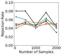
(a) Mean shift $d=10$

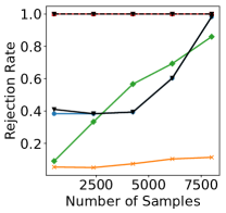
(b) Blobs $d=2$

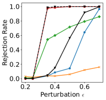
(c) RBM $d=20$

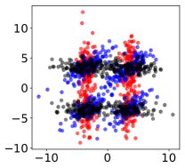
(d) Blobs problem.

Figure 1: Rejection rates (estimated from 300 trials) for the six tests with $\alpha=0.05$ is shown. “MMD-U” refers to the usage of the complete U-statistic for MMD which is $\widehat{\mathrm{MMD}}^{2}_{u}$, “MMD-Lin” refers to the linear time estimator $\widehat{\mathrm{MMD}}^{2}_{l}$ and similarly for KSD Complete and KSD Linear (defined in Section 2).

In this section, we demonstrate our proposed method for both toy problems and real world datasets. Our first experiment is a baseline comparison of our proposed method RelPSI to RelMMD [4] and RelKSD (see Appendix D). In this experiment, we consider a fixed hypothesis of model comparison for two candidate models (RelMulti is not applicable here). This is the original setting that RelMMD was proposed for. In the second experiment, we consider a set of mixture models for smiling and non-smiling images of CelebA [24] where each model has its own unique generating proportions from the real data set or images from trained GANs. For our final experiment, we examine density estimation models trained on the Chicago crime dataset considered by Jitkrittum et al. [19]. In this experiment, each model has a score function which allows us to apply both RelPSI and RelMulti with KSD. In the last two experiments on real data, there is no ground truth for which candidate model is the best; so estimating TPR, FDR and FPR is infeasible. Instead, the experiments are designed to have a strong indication of the ground truth with support from another metric. More synthetic experiments are shown in Appendix H to verify our theoretical results. In order to account for sample variability, our experiments are averaged over at least $100$ trials with new samples (from a different seed) redrawn for each trial. Code for reproducing the results is online.

1. A comparison of RelMMD, RelKSD, RelPSI-KSD and RelPSI-MMD ($l=2$): The aim of this experiment is to investigate the behaviour of the proposed tests with RelMMD and RelKSD as baseline comparisons and empirically demonstrate that RelPSI-MMD and RelPSI-KSD possess desirable properties such as level-$\alpha$ and comparable test power. Since RelMMD and RelKSD have no concept of selection, in order for the results to be comparable we fixed null hypothesis to be $H_{0}:D(P_{1},R)\leq D(P_{2},R)$ which is possible for RelPSI by fixing $\bm{\eta}^{\top}=[-1,1]$. In this experiment, we consider the following problems:

1. Mean shift: The two candidate models are isotropic Gaussians on $\mathbb{R}^{10}$ with varying mean: $P_{1}=\mathcal{N}([0.5,0,\cdots,0],\bm{I})$ and $P_{2}=\mathcal{N}([-0.5,0,\cdots,0],\bm{I})$. Our reference distribution is $R=\mathcal{N}(\bm{0},\bm{I})$. In this case, $H_{0}$ is true.

2. Blobs: This problem was studied by various authors [7, 15, 17]. Each distribution is a mixture of Gaussians with a similar structure on a global scale but different locally by rotation. Samples from this distribution is shown in Figure 1d. In this case, the $H_{1}$ is true.

3. Restricted Boltzmann Machine (RBM): This problem was studied by [23, 19, 17]. Each distribution is given by a Gaussian Restricted Boltzmann Machine (RBM) with a density $p(\bm{y})=\sum_{\bm{x}}p^{\prime}(\bm{y},\bm{x})$ and $p^{\prime}(\bm{y},\bm{x})=\frac{1}{Z}\exp(\bm{y^{\top}Bx}+\bm{b^{\top}y}+\bm{c^{\top}x}-\frac{1}{2}||\bm{y}||^{2})$ where $\bm{x}$ are the latent variables and model parameters are $\bm{B,b,c}$. The model will share the same parameters $\bm{b}$ and $\bm{c}$ (which are drawn from a standard normal) with the reference distribution but the matrix $\bm{B}$ (sampled uniformly from $\{-1,1\}$) will be perturbed with $\bm{B}^{p_{2}}=\bm{B}+0.3\delta$ and $\bm{B}^{p_{1}}=\bm{B}+\epsilon\delta$ where $\epsilon$ varies between $0$ and $1$. It measures the sensitivity of the test [19] since perturbing only one entry can create a difference that is hard to detect. Furthermore, We fix $n=1000$, $d_{x}=5$, $d_{y}=20$.

Our proposal and baselines are all non-parametric kernel based test. For a fair comparison, all the tests use the same Gaussian kernel with its bandwidth chosen by the median heuristic. In Figure 1, it shows the rejection rates for all tests. As expected, the tests based on KSD have higher power than MMD due to having access to the density function. Additionally, linear time estimators perform worse than their complete counterpart.

In Figure 1a, when $H_{0}$ is true, then the false rejection rate (type-I error) is controlled around level $\alpha$ for all tests. In Figure 1b, the poor performance of MMD-based tests in blobs experiments is caused by an unsuitable choice of bandwidth. The median heuristic cannot capture the small-scale differences [15, 17]. Even though KSD-based tests utilize the same heuristic, equipped with the density function a mismatch in the distribution shape can be detected. Interestingly, in all our experiments, the RelPSI variants perform comparatively to their cousins, Rel-MMD and Rel-KSD but as expected, the power is lowered due to the loss of information from our conditioning [9]. These two problems show the behaviour of the tests when the number of samples $n$ increases.

In Figure 1c, this shows the behaviour of the tests when the difference between the candidate models increases (one model gets closer to the reference distribution). When $\epsilon<0.3$, the null case is true and the tests exhibit a low rejection rate. However, when $\epsilon>0.3$ then the alternative is true. Tests utilizing KSD can detect this change quickly which indicated by the sharp increase in the rejection rate when $\epsilon=0.3$. However, MMD-based tests are unable to detect the differences at that point. As the amount of perturbation increases, this changes and MMD tests begin to identify with significance that the alternative is true. Here we see that RelPSI-MMD has visibly lowered rejection rate indicating the cost of power for conditioning, whilst for RelPSI-KSD and RelKSD both have similar power.

Table 1: A comparison of our proposed method with FID. The underlying distribution are samples forming a mixture of smiling (S) or non-smiling (N) faces which can be either generated (G) or real (R). “Rej.” denotes the rate of rejection of the model indicating that it is significantly worse than the best model. “Sel.” is the rate at which the model is selected (the one with the minimum discrepancy score). Average FID scores are also reported. These results are averaged over 100 trials.

	Mix		RelPSI-MMD		RelMulti-MMD		FID
Model	S	N	Rej.	Sel.	Rej.	Sel.	Aver.	Sel.
1	0.50 (G)	0.50 (G)	0.99	0.0	1.0	0.0	$27.86\pm 0.49$	0
2	0.60 (R)	0.40 (R)	0.39	0.02	0.18	0.08	$16.01\pm 0.19$	0.39
3	0.40 (R)	0.60 (R)	0.28	0.03	0.19	0.10	$16.29\pm 0.20$	0.03
4	0.51 (R)	0.49 (R)	0.02	0.52	0.03	0.37	$16.03\pm 0.18$	0.27
5	0.52 (R)	0.48 (R)	0.06	0.43	0.0	0.45	$16.01\pm 0.17$	0.31
Truth	0.5 (R)	0.5 (R)	-	-	-	-	-	-

2. Image Comparison $l=5$: In this experiment, we apply our proposed test RelPSI-MMD and RelMulti-MMD for comparing between five image generating candidate models. We consider the CelebA dataset [24] which for each sample is an image of a celebrity labelled with 40 annotated features. As our reference distribution and candidate models, we use a mixture of smiling and non-smiling faces of varying proportions (Shown in Table 1) where the model can generate images from a GAN or from the real dataset. For generated images, we use the GANs of [17, Appendix B]. In each trial, $n=2000$ samples are used. We partition the dataset such that the reference distribution draws distinct independent samples, and each model samples independently of the remainder of the pool. All algorithms receive the same model samples. The kernel used is the Inverse Multiquadric (IMQ) on 2048 features extracted by the Inception-v3 network at the pool layer [30]. Additionally, we use 50:50 split for RelMulti-MMD. Our baseline is the procedure of choosing the lowest Fréchet Inception Distance (FID) [16]. We note the authors did not propose a statistical test with FID. Table 1 summaries the results from the experiment.

In Table 1, we report the model-wise rejection rate (a high rejection indicts a poor candidate relatively speaking) and the model selection rate (which indicates the rate that the model has the smallest discrepancy from the given samples). The table illustrates several interesting points. First, even though Model 1 shares the same portions as the true reference models, the quality of the generated images is a poor match to the reference images and thus is frequently rejected. A considerably higher FID score (than the rest) also supports this claim. Secondly, in this experiment, MMD is a good estimator of the best model for both RelPSI and RelMulti (with splitting exhibiting higher variance) but the minimum FID score selects the incorrect model $73\%$ of the time. The additional testing indicate that Model 4 or Model 5 could be the best as they were rarely deemed worse than the best which is unsurprising given that their mixing proportions are closest to the true distribution. The low rejection for Model 4 is expected given that they differ by only $40$ samples. Model 2 and 3 have respectable model-wise rejections to indicate their position as worse than the best. Overall, both RelPSI and RelMulti perform well and shows that the additional testing phase yields more information than the approach of picking the minimum of a score function (especially for FID).

3. Density Comparison $l=5$: In our final experiment, we demonstrate RelPSI-KSD and RelMulti-KSD on the Chicago data-set considered in Jitkrittum et al. [19] which consists of $11957$ data points. We split the data-set into disjoint sets such that $7000$ samples are used for training and the remainder for testing. For our candidate models, we trained a Mixture of Gaussians (MoG) with expectation maximization with $C$ components where $C\in\{1,2,5\}$, Masked Auto-encoder for Density Estimation (MADE) [12] and a Masked Auto-regressive Flow (MAF) [25]. MAF with 1 autoregressive layer with a standard normal as the base distribution (or equivalently MADE) and MAF model has 5 autoregressive layers with a base distribution of a MoG (5). Each autoregressive layer is a feed-forward network with 512 hidden units. Both invertible models are trained with maximum likelihood with a small amount of $\ell_{2}$ penalty on the weights. In each trial, we sample $n=2000$ points independently of the test set. The resultant density shown in Figure 2 and the reference distribution in Figure 2a. We compare our result with the negative log-likelihood (NLL). Here we use the IMQ kernel.

The results are shown in Table 2. If performance is measured by a higher model-wise rejection rates, for this experiment RelPSI-KSD performs better than RelMulti-KSD. RelPSI-KSD suggests that MoG (1), MoG (2) and MADE are worse than the best but is unsure about MoG (5) and MAF. Whilst the only significant rejection of RelMulti-KSD is MoG (1). These findings with RelPSI-KSD can be further endorsed by inspecting the density (see Figure 2). It is clear that MoG (1), MoG (2) and MADE are too simple. But between MADE and MAF (5), it is unclear which is a better fit. Negative Log Likelihood (NLL) consistently suggest that MAF is the best which corroborates with our findings that MAF is one of the top models. The preference of MAF for NLL is due to log likelihood not penalizing the complexity of the model (MAF is the most complex with the highest number of parameters).

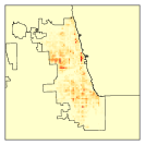
(a) Truth

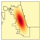
(b) MoG (1)

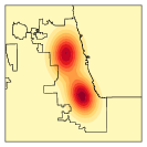
(c) MoG (2)

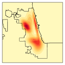
(d) MoG (5)

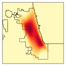
(e) MADE

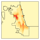
(f) MAF

Figure 2: The density plots of the trained models on the Chicago Crime dataset.

	RelPSI-KSD		RelMul-KSD		NLL
Model	Rej.	Sel.	Rej.	Sel.	Aver.	Sel.
MoG (1)	0.42	0.	0.22	0	2.64	0
MoG (2)	0.28	0.01	0.07	0.08	2.55	0
MoG (5)	0.02	0.62	0	0.38	2.38	0
MADE	0.26	0.01	0.04	0.03	2.53	0
MAF (5)	0	0.36	0	0.51	2.25	1.

Table 2: Relative testing on unconditional density estimation models. The model-wise rejection rates, selection rates and Negative Log Likelihood (NLL) scores are reported. These results are averaged over 100 trials.

Acknowledgments

M.Y. was supported by the JST PRESTO program JPMJPR165A and partly supported by MEXT KAKENHI 16H06299 and the RIKEN engineering network funding.

Kernel Stein Tests for Multiple Model Comparison

Supplementary

Appendix A Definitions and FPR proof

In this section, we define TPR and FPR, and prove that our proposals control FPR.

Recall the definitions of $\mathcal{I}_{-}$ and $\mathcal{I}_{+}$ (see Section 3.3). $\mathcal{I}_{-}$ is the set of models that are not worse than $P_{J}$ (the true best model). $\mathcal{I}_{+}$ is the set of models that are worse than $P_{J}$. We say that an algorithm decides that a model $P_{i}$ is positive if it decides that $P_{i}$ is worse than $P_{J}$. We define true positive rate (TPR) and false positive rate (FPR) to be

$$\mathrm{FPR}=\frac{1}{|\mathcal{I}_{-}|}\mathbb{E}[|\{i\in\mathcal{I}_{-}:\text{ the algorithm decides that $P_{i}$ is positive}\}|],$$

$$\mathrm{TPR}=\frac{1}{|\mathcal{I}_{+}|}\mathbb{E}[|\{i\in\mathcal{I}_{+}:\text{ the algorithm decides that $P_{i}$ is positive}\}|].$$

Both TPR and FPR can be estimated by averaging the TPR and FPR with multiple independent trials (as was done in Experiment H). We call this quantity the empirical TPR and FPR, denoted as $\widehat{\mathrm{TPR}}$ and $\widehat{\mathrm{FPR}}$ respectively.

The following lemma shows that our proposals controls FPR.

See 4.2

Proof.

From law of total expectation, we have

$$\mathrm{FPR} =\frac{1}{|\mathcal{I}_{-}|}\mathbb{E}[|\{i\in\mathcal{I}_{-}:\text{ the algorithm decides that $i$ is positive}\}|]$$

$$=\frac{1}{|\mathcal{I}_{-}|}\mathbb{E}[\mathbb{E}[|\{i\in\mathcal{I}_{-}:\text{ the algorithm decides that $i$ is positive}\}|\,|\,P_{\hat{J}}\text{ is selected}]]$$

$$=\frac{1}{|\mathcal{I}_{-}|}\mathbb{E}[\mathbb{E}[\sum_{i\in\mathcal{I}_{-}}\mathbb{I}(\text{The algorithm decides that $i$ is positive})\,|\,P_{\hat{J}}\text{ is selected}]]$$

$$=\frac{1}{|\mathcal{I}_{-}|}\mathbb{E}[\sum_{i\in\mathcal{I}_{-}}\mathbb{P}(\text{The algorithm decides that $i$ is positive}\,|\,P_{\hat{J}}\text{ is selected})]$$

$$=\frac{1}{|\mathcal{I}_{-}|}\mathbb{E}[\sum_{i\in\mathcal{I}_{-}}\mathbb{P}(\sqrt{n}[\hat{D}(P_{i},R)-\hat{D}(P_{\hat{J}},R)]>\hat{t}_{\alpha}\,|\,\hat{J}\text{ is selected})]$$

$$\leq\frac{1}{|\mathcal{I}_{-}|}\mathbb{E}[\sum_{i\in\mathcal{I}_{-}}\alpha]$$

$$=\frac{1}{|\mathcal{I}_{-}|}\mathbb{E}\big{[}|I_{-}|\alpha\big{]}$$

$$=\alpha,$$

where $\mathbb{I}$ is the indicator function. ∎

Appendix B Algorithms

Algorithms for RelPSI (see Algorithm 1) and RelMulti (see Algorithm 2) proposed in Section 3 are provided in this section.

Algorithm 1 RelPSI $H_{0,i}:D(P_{\hat{J}},R)\geq D(P_{i},R)\ |\ P_{\hat{J}}$ is selected.

1:procedure RelPSI($\mathcal{M},R,\alpha$)

2:     Estimate $\hat{\bm{\Sigma}}$ given in Theorem C.1 and Theorem C.2 for KSD and MMD respectively.

3:     $\bm{r}\leftarrow(0,\ldots,0)\in\{0,1\}^{l}$

4:     $\bm{z}\leftarrow[\sqrt{n}\hat{D}(P_{1},R),\sqrt{n}\hat{D}(P_{2},R),\ldots,\sqrt{n}\hat{D}(P_{l},R)]^{\top}$

5:     $\hat{J}\leftarrow\arg\min_{j\in\mathcal{I}}\hat{D}(P_{j},R)$.

6:     Compute $\bm{A}$ and $\bm{b}$ (as defined in Section 3.1).

7:     for $i\in\mathcal{I}:i\neq\hat{J}$ do

8:         $\bm{\eta}\leftarrow[0,\ldots,\overbrace{-1}^{\hat{J}},\ldots,\overbrace{1}^{i},\ldots,0]^{\top}$

9:         $\hat{\sigma}\leftarrow\sqrt{\bm{\eta}^{\top}\hat{\bm{\Sigma}}\bm{\eta}}$

10:         Compute $\mathcal{V}^{+}$ and $\mathcal{V}^{-}$ (described in Lemma 3.1).

11:         $\hat{t}_{\alpha}\leftarrow\hat{\sigma}\Phi^{-1}\bigg{(}(1-\alpha)\Phi\left(\frac{{\mathcal{V^{+}}}}{\hat{\sigma}}\right)+\alpha\Phi\left(\frac{{\mathcal{V^{-}}}}{\hat{\sigma}}\right)\bigg{)}$

12:          $\bm{r}_{i}\leftarrow\bm{\eta}^{\top}\bm{z}>\hat{t}_{\alpha}$

13:     end for

14:return $\bm{r}$

15:end procedure

Algorithm 2 RelMulti $H_{0,i}:D(P_{\hat{J}},R)\geq D(P_{i},R)\ |\ P_{\hat{J}}$ is selected.

1:procedure RelMulti($\mathcal{M},R,\alpha,\rho$)

2:     Estimate $\hat{\bm{\Sigma}}$ as given in Theorem C.1 and Theorem C.2 for KSD and MMD respectively.

3:     $\mathcal{D}_{0},\,\mathcal{D}_{1}\leftarrow$ SplitData($\mathcal{M},R,\rho$)

4:     $n_{1}\leftarrow\rho n$

5:     (With $\mathcal{D}_{0}$) $\hat{J}\leftarrow\arg\min_{j\in\mathcal{I}}\hat{D}(P_{j},R)$.

6:     Compute $\bm{A}$ and $\bm{b}$.

7:     for $i\in\mathcal{I}:i\neq\hat{J}$ do (with $\mathcal{D}_{1}$)

8:         Compute $\bm{z}_{2}=[\sqrt{n_{1}}\hat{D}(P_{1},R),\sqrt{n_{1}}\hat{D}(P_{2},R),\ldots,\sqrt{n_{1}}\hat{D}(P_{l},R)]^{\top}$

9:         $\bm{\eta}^{\top}=[0,\ldots,\overbrace{-1}^{\hat{J}}\ldots,\overbrace{1}^{i},\ldots,0]$

10:         $\hat{\sigma}\leftarrow\sqrt{\bm{\eta}^{\top}\hat{\bm{\Sigma}}\bm{\eta}}$

11:         $\bm{p}_{i}\leftarrow 1-\Phi(\frac{\bm{\eta}^{\top}\bm{z}_{2}}{\hat{\sigma}})$

12:     end for

13:return FDRCorrection($\bm{p},\alpha$)

14:end procedure

In algorithm 2, FDRCorrection($\bm{p},\alpha$) takes a list of $p$-values $\bm{p}$ and returns a list of rejections for each element of $\bm{p}$ such that the false discovery rate is controlled at $\alpha$. In our experiments, we use the Benjamini–Yekutieli procedure [1]. SplitData($\mathcal{M},R,\rho$) is a function that splits the samples generated by $R$ and $\mathcal{M}$ (if it is represented by samples). It returns two datasets $\mathcal{D}_{0}$ and $\mathcal{D}_{1}$ such that $|\mathcal{D}_{0}|=(1-\rho)n$ and $|\mathcal{D}_{1}|=\rho n$.

Appendix C Asymptotic distributions

In this section, we prove the asymptotic distribution of $\widehat{\mathrm{KSD}}^{2}_{u}$ and also provide the asymptotic distribution of $\widehat{\mathrm{MMD}}^{2}_{u}$ for completeness.

Theorem C.1 (Asymptotic Distribution of $\savestack{\tmpbox}{\stretchto{\scaleto{\scalerel*[\widthof{\mathrm{KSD}^{2}_{u}}]{\kern-0.6pt\bigwedge\kern-0.6pt}{\rule[-505.89pt]{4.30554pt}{505.89pt}}}{}}{0.5ex}}\stackon[1pt]{\mathrm{KSD}^{2}_{u}}{\tmpbox}$).

Let $P_{i},P_{j}$ be distributions with density functions $p_{i},p_{j}$ respectively, and let $R$ be the data generating distribution. Assume that $P_{i},P_{j},R$ are distinct. We denote a sample by $Z_{n}=Z\sim R$. $\sqrt{n}\Bigg{(}\begin{pmatrix}\savestack{\tmpbox}{\stretchto{\scaleto{\scalerel*[\widthof{\mathrm{KSD}}]{\kern-0.6pt\bigwedge\kern-0.6pt}{\rule[-505.89pt]{4.30554pt}{505.89pt}}}{}}{0.5ex}}\stackon[1pt]{\mathrm{KSD}}{\tmpbox}^{2}_{u}(P_{i},Z)\\ \savestack{\tmpbox}{\stretchto{\scaleto{\scalerel*[\widthof{\mathrm{KSD}}]{\kern-0.6pt\bigwedge\kern-0.6pt}{\rule[-505.89pt]{4.30554pt}{505.89pt}}}{}}{0.5ex}}\stackon[1pt]{\mathrm{KSD}}{\tmpbox}^{2}_{u}(P_{j},Z)\end{pmatrix}-\begin{pmatrix}\mathrm{KSD}^{2}(P_{i},R)\\ \mathrm{KSD}^{2}(P_{j},R)\end{pmatrix}\Bigg{)}\xrightarrow{d}\mathcal{N}(\bm{0},\bm{\Sigma}),$ where $\bm{\Sigma}=\begin{pmatrix}\sigma^{2}_{P_{i}R}\quad\sigma_{P_{i}RP_{j}R}\\ \sigma_{P_{i}RP_{j}R}\quad\sigma^{2}_{P_{j}R}\\ \end{pmatrix},\ \sigma_{P_{i}RP_{j}R}=\mathrm{Cov}_{x\sim R}[\mathbb{E}_{x^{\prime}\sim R}[u_{p_{i}}(x,x^{\prime})],\mathbb{E}_{x^{\prime}\sim R}[u_{p_{j}}(x,x^{\prime})]]$ and $\sigma^{2}_{P_{i}R}=\mathrm{Var}_{x^{\prime}\sim R}[\mathbb{E}_{x^{\prime}\sim R}[u_{p_{i}}(x,x^{\prime})]$.

Proof.

Let $\mathcal{\mathcal{\mathcal{\mathcal{{X}}}}}=\{x_{i}\}_{i=1}^{n}$ be $n$ i.i.d. random variables drawn from $R$ and we have a model with its corresponding gradient of its log density $s_{P_{i}}(x)=\nabla_{x}\log p_{i}(x)$. The complete U-statistic estimate of KSD between $P_{i}$ and $R$ is

$$\savestack{\tmpbox}{\stretchto{\scaleto{\scalerel*[\widthof{\mathrm{KSD}}]{\kern-0.6pt\bigwedge\kern-0.6pt}{\rule[-505.89pt]{4.30554pt}{505.89pt}}}{}}{0.5ex}}\stackon[1pt]{\mathrm{KSD}}{\tmpbox}_{u}^{2}(P_{i},R)=\mathbb{E}_{x,x^{\prime}\sim R}[u_{p_{i}}(x,x^{\prime})]\approx\frac{{1}}{n_{2}}\sum_{i\neq j}^{n}u_{p_{i}}(x_{i},x_{j})$$

where $u_{p_{i}}(x,y)=s_{p_{i}}(x)^{\top}s_{p_{i}}(y)k(x,y)+s_{p_{i}}(y)^{\top}\nabla_{x}k(x,y)+s_{p_{i}}(x)^{\top}\nabla_{y}k(x,y)+\operatorname{tr}[\nabla_{x,y}k(x,y)]$ and $n_{2}=n(n-1)$.

Similarly, for another model $P_{j}$ and its gradient of its log density $s_{P_{j}}(x)=\nabla_{x}\log p_{j}(x)$. Its estimator is

$$\savestack{\tmpbox}{\stretchto{\scaleto{\scalerel*[\widthof{\mathrm{KSD}}]{\kern-0.6pt\bigwedge\kern-0.6pt}{\rule[-505.89pt]{4.30554pt}{505.89pt}}}{}}{0.5ex}}\stackon[1pt]{\mathrm{KSD}}{\tmpbox}_{u}^{2}(P_{j},R)=\mathbb{{E}}_{x,x^{\prime}\sim R}[u_{p_{j}}x,x^{\prime})]\approx\frac{{1}}{n_{2}}\sum_{i\neq j}^{n}u_{p_{j}}(x_{i},x_{j})$$

where $u_{p_{j}}(x,y)=s_{p_{j}}(x)^{\top}s_{p_{j}}(y)k(x,y)+s_{p_{j}}(y)^{\top}\nabla_{x}k(x,y)+s_{p_{j}}(x)^{\top}\nabla_{y}k(x,y)+\operatorname{tr}[\nabla_{x,y}k(x,y)]$.

The covariance matrix of a U-statistic with a kernel of order 2 is

$$\bm{\Sigma}=\frac{4(n-2)}{n(n-1)}\bm{\zeta}+\mathcal{O}_{p}(n^{-2})$$

where, for the variance term and covariance term, we have $\zeta_{ii}=\mathrm{Var}_{x\sim R}(\mathbb{{E}}_{y\sim R}[u_{p_{i}}(x,y)])$ and $\zeta_{ij}=\mathrm{Cov}_{x\sim R}(\mathbb{{E}}_{y\sim R}[u_{p_{i}}(x,y)],\mathbb{{E}}_{y\sim R}[u_{p_{j}}(x,y)])$ respectively. ∎

The asymptotic distribution is provided below and is shown to be the case by Bounliphone et al. [4].

Theorem C.2 (Asymptotic Distribution of $\savestack{\tmpbox}{\stretchto{\scaleto{\scalerel*[\widthof{\mathrm{MMD}}]{\kern-0.6pt\bigwedge\kern-0.6pt}{\rule[-505.89pt]{4.30554pt}{505.89pt}}}{}}{0.5ex}}\stackon[1pt]{\mathrm{MMD}}{\tmpbox}^{2}_{u}$ [4]).

Assume that $P_{i}$, $P_{j}$ and $R$ are distinct. We denote samples $X\sim P_{i}$, $Y\sim P_{j}$, $Z\sim R$.

$$\sqrt{n}\bigg{(}\begin{pmatrix}\savestack{\tmpbox}{\stretchto{\scaleto{\scalerel*[\widthof{\mathrm{MMD}}]{\kern-0.6pt\bigwedge\kern-0.6pt}{\rule[-505.89pt]{4.30554pt}{505.89pt}}}{}}{0.5ex}}\stackon[1pt]{\mathrm{MMD}}{\tmpbox}^{2}_{u}(P_{i},Z)\\ \savestack{\tmpbox}{\stretchto{\scaleto{\scalerel*[\widthof{\mathrm{MMD}}]{\kern-0.6pt\bigwedge\kern-0.6pt}{\rule[-505.89pt]{4.30554pt}{505.89pt}}}{}}{0.5ex}}\stackon[1pt]{\mathrm{MMD}}{\tmpbox}^{2}_{u}(P_{j},Z)\end{pmatrix}-\begin{pmatrix}\mathrm{MMD}^{2}(P_{i},R)\\ \mathrm{MMD}^{2}(P_{j},R)\end{pmatrix}\bigg{)}\xrightarrow{d}\mathcal{N}(\bm{0},\bm{\Sigma})$$

where $\bm{\Sigma}=\begin{pmatrix}\sigma^{2}_{P_{i}R}\quad\sigma_{P_{i}RP_{j}R}\\ \sigma_{P_{i}RP_{j}R}\quad\sigma^{2}_{P_{j}R}\\ \end{pmatrix}$ and $\sigma_{P_{i}RP_{j}R}=\mathrm{Cov}[\mathbb{E}_{x^{\prime}\sim P_{i}\times R}[h(X,x^{\prime})],\mathbb{E}_{x^{\prime}\sim P_{j}\times R}[g(X,x^{\prime})]]$ and $\sigma^{2}_{P_{j}R}=\mathrm{Var}[\mathbb{E}_{x^{\prime}\sim P_{j}\times R}[h(X,x^{\prime})]$.

Appendix D Relative Kernelized Stein Discrepancy (RelKSD)

In this section, we describe the testing procedure for relative tests with KSD (a simple extension of RelMMD [4]). Currently, there is no test of relative fit with Kernelized Stein Discrepancy, and so we propose such a test using the complete estimator $\savestack{\tmpbox}{\stretchto{\scaleto{\scalerel*[\widthof{\mathrm{KSD}}]{\kern-0.6pt\bigwedge\kern-0.6pt}{\rule[-505.89pt]{4.30554pt}{505.89pt}}}{}}{0.5ex}}\stackon[1pt]{\mathrm{KSD}}{\tmpbox}^{2}_{u}$ which we call RelKSD. The test mirrors the proposal of Bounliphone et al. [4] and, given the asymptotic distribution of $\savestack{\tmpbox}{\stretchto{\scaleto{\scalerel*[\widthof{\mathrm{KSD}}]{\kern-0.6pt\bigwedge\kern-0.6pt}{\rule[-505.89pt]{4.30554pt}{505.89pt}}}{}}{0.5ex}}\stackon[1pt]{\mathrm{KSD}}{\tmpbox}^{2}_{u}$, it is a simple extension since its cross-covariance is known (see Theorem C.1).

Given two candidate models $P_{1}$ and $P_{2}$ with a reference distribution $R$ with its samples denoted as $Z\sim R$, we define our test statistic as $\sqrt{n}[\savestack{\tmpbox}{\stretchto{\scaleto{\scalerel*[\widthof{\mathrm{KSD}}]{\kern-0.6pt\bigwedge\kern-0.6pt}{\rule[-505.89pt]{4.30554pt}{505.89pt}}}{}}{0.5ex}}\stackon[1pt]{\mathrm{KSD}}{\tmpbox}^{2}_{u}(P_{1},Z)-\savestack{\tmpbox}{\stretchto{\scaleto{\scalerel*[\widthof{\mathrm{KSD}}]{\kern-0.6pt\bigwedge\kern-0.6pt}{\rule[-505.89pt]{4.30554pt}{505.89pt}}}{}}{0.5ex}}\stackon[1pt]{\mathrm{KSD}}{\tmpbox}^{2}_{u}(P_{2},Z)]$. For the test of relative similarity, we assume that the candidate models ($P_{1}$ and $P_{2}$) and unknown generating distribution $R$ are all distinct. Then, under the null hypothesis $H_{0}:\mathrm{KSD}^{2}(P_{1},R)-\mathrm{KSD}^{2}(P_{2},R)\leq 0$, we can derive the asymptotic null distribution as follows. By the continuous mapping theorem and Theorem C.1, we have

$$\sqrt{n}[\savestack{\tmpbox}{\stretchto{\scaleto{\scalerel*[\widthof{\mathrm{KSD}}]{\kern-0.6pt\bigwedge\kern-0.6pt}{\rule[-505.89pt]{4.30554pt}{505.89pt}}}{}}{0.5ex}}\stackon[1pt]{\mathrm{KSD}}{\tmpbox}^{2}_{u}(P_{1},Z)-\savestack{\tmpbox}{\stretchto{\scaleto{\scalerel*[\widthof{\mathrm{KSD}}]{\kern-0.6pt\bigwedge\kern-0.6pt}{\rule[-505.89pt]{4.30554pt}{505.89pt}}}{}}{0.5ex}}\stackon[1pt]{\mathrm{KSD}}{\tmpbox}^{2}_{u}(P_{2},Z)]-\sqrt{n}[\mathrm{KSD}^{2}(P_{1},R)-\mathrm{KSD}^{2}(P_{2},R)]\xrightarrow{d}\mathcal{N}\bigg{(}0,\sigma^{2}\bigg{)}$$

where $\sigma^{2}=\begin{pmatrix}1\\ -1\end{pmatrix}^{\top}\bm{\Sigma}\begin{pmatrix}1\\ -1\end{pmatrix}=\sigma^{2}_{P_{1}R}-2\sigma_{P_{1}RP_{2}R}+\sigma^{2}_{P_{2}R},$ and $\bm{\Sigma}$ is defined in Theorem C.1 (which we assume is positive definite). We will also use the most conservative threshold by letting the rejection threshold $t_{\alpha}$ be the $(1-\alpha)$-quantile of the asymptotic distribution of $\sqrt{n}[\savestack{\tmpbox}{\stretchto{\scaleto{\scalerel*[\widthof{\mathrm{KSD}}]{\kern-0.6pt\bigwedge\kern-0.6pt}{\rule[-505.89pt]{4.30554pt}{505.89pt}}}{}}{0.5ex}}\stackon[1pt]{\mathrm{KSD}}{\tmpbox}^{2}_{u}(P_{1},Z)-\savestack{\tmpbox}{\stretchto{\scaleto{\scalerel*[\widthof{\mathrm{KSD}}]{\kern-0.6pt\bigwedge\kern-0.6pt}{\rule[-505.89pt]{4.30554pt}{505.89pt}}}{}}{0.5ex}}\stackon[1pt]{\mathrm{KSD}}{\tmpbox}^{2}_{u}(P_{2},Z)]$ with mean zero (see Bounliphone et al.[4]). If our statistic is above the $t_{\alpha}$, we reject the null.

Appendix E Calibration of the test

In this section, we will show that the p-values obtained are well calibrated, when two distributions are equal, measured by either MMD or KSD. The distribution of p-values should be uniform. Figure 3 shows the empirical CDF of p-values and should lie on the line if it is calibrated. Additionally, we show the empirical distribution of p values for a three of different mean shift problems where observed distribution is $R=\mathcal{N}(0,1)$ and our candidate models are $P_{1}=\mathcal{N}(\mu_{1},1)$ and $P_{2}=\mathcal{N}(\mu_{2},1)$

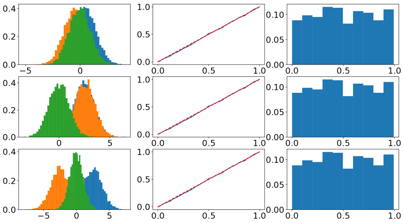
Figure 3: Mean shift experiment described in experiments with (a) $\mu_{1}=0.5$ and $\mu_{2}=-0.5$, (b) $\mu_{1}=2.5$ and $\mu_{2}=2.5$, (c) $\mu_{1}=2.5$ and $\mu_{2}=-2.5$.

Appendix F Performance analysis for two models

In this section, we analyse the performance of our two proposed methods: RelPSI and RelMulti for $l=2$ candidate models. We begin by computing the probability that we select the best model correctly (and selecting incorrectly). Then provide a closed form formula for computing the rejection threshold, and from this we were able to characterize the probability of rejection and proof our theoretical result.

F.1 Cumulative distribution function of a truncated normal

The cumulative distribution function (CDF) of a truncated normal is given by

$$\Psi(x\,|\>\mu,\sigma,\mathcal{V}^{-},\mathcal{V}^{+})=\frac{{\Phi(\frac{{x-\mu}}{\sigma})-\Phi(\frac{{\mathcal{V}^{-}-\mu}}{\sigma})}}{\Phi(\frac{{\mathcal{V}^{+}-\mu}}{\sigma})-\Phi(\frac{{\mathcal{V}^{-}-\mu}}{\sigma})},$$

where $\Phi$ is the CDF of the standard normal distribution [5, Section 3.3].

F.2 Characterizing the selection event

Under the null and alternative hypotheses, for both $\widehat{\mathrm{MMD}}_{u}^{2}(P,R)$ and $\widehat{\mathrm{{KSD}}}_{u}^{2}(P,R)$, the test statistic is asymptotically normal i.e., for a sufficiently large $n$, we have

$$\sqrt{{n}}\big{[}\hat{D}(P_{2},R)-\hat{D}(P_{1},R)-\mu\big{]}\sim\mathcal{{N}}(0,\sigma^{2}),$$

where $\mu:=D(P_{2},R)-D(P_{1},R)$ is the population difference and $D(\cdot,\cdot)$ can be either $\mathrm{MMD}^{2}$ or $\mathrm{KSD}^{2}$. The probability of selecting the model $P_{1}$, i.e., $P_{\hat{J}}=P_{1}$, is equivalent to the probability of observing $\hat{D}(P_{1},R)<\hat{D}(P_{2},R)$. The following lemma derives this quantity.

Lemma F.1.

Given two models $P_{1}$ and $P_{2}$, and the test statistic $\sqrt{{n}}[\hat{D}(P_{2},R)-\hat{D}(P_{1},R)]$ such that $\sqrt{{n}}\big{[}\hat{D}(P_{2},R)-\hat{D}(P_{1},R)-\mu\big{]}\stackrel{{\scriptstyle d}}{{\to}}\mathcal{{N}}(0,\sigma^{2})$, where $\mu:=D(P_{2},R)-D(P_{1},R)$, then the probability that we select $P_{1}$ as the reference is

$$\mathbb{P}(P_{\hat{J}}=P_{1})=\mathbb{P}(\hat{D}(P_{1},R)<\hat{D}(P_{2},R))\approx\Phi\left(\frac{\sqrt{n}\mu}{\sigma}\right).$$

It follows that $\mathbb{P}(P_{\hat{J}}=P_{2})\approx\Phi(-\frac{\sqrt{{n}}{\mu}}{\sigma})$.

Proof.

For some sufficiently large $n$, we have

$$\mathbb{P}(P_{\hat{J}}=P_{1}) =\mathbb{P}(\sqrt{{n}}\hat{D}(P_{1},R)<\sqrt{{n}}\hat{D}(P_{2},R))$$

$$=\mathbb{P}(\sqrt{{n}}[\hat{D}(P_{2},R)-\hat{D}(P_{1},R)]>0)$$

$$\approx 1-\Phi(-\frac{\sqrt{n}{\mu}}{\sigma})=\Phi\left(\frac{\sqrt{n}\mu}{\sigma}\right),$$

and $\mathbb{P}(P_{\hat{J}}=P_{2})=1-\mathbb{P}(P_{\hat{J}}=P_{1})\approx\Phi(-\frac{\sqrt{{n}}{\mu}}{\sigma}).$ ∎

It can be seen that as $n$ gets larger the selection procedure is more likely to select the correct model.

F.3 Truncation points of RelPSI

To study the performance of RelPSI, it is necessary to characterize the truncation points in the polyhedral lemma (Theorem 3.1). In the case of two candidate models, the truncation points are simple as shown in Lemma F.2.

Lemma F.2.

Consider two candidate models $P_{1}$ and $P_{2}$ and the selection algorithm described in Section 3.1, with the test statistic $\sqrt{n}[\hat{D}(P_{2},R)-\hat{D}(P_{1},R)]$. The upper truncation point $\mathcal{V}^{+}$ and lower truncation point $\mathcal{V}^{-}$ (see Theorem 3.1) when the selection procedure observes $\hat{D}(P_{1},R)<\hat{D}(P_{2},R)$, i.e., $P_{\hat{J}}=P_{1}$, are

$$\mathcal{V}^{-}=0,\ \mathcal{V}^{+}=\infty.$$

When the selection procedure observes $\hat{D}(P_{2},R)<\hat{D}(P_{1},R)$, i.e., $P_{\hat{J}}=P_{2}$, then the truncation points are

$$\mathcal{V}^{-}=-\infty,\ \mathcal{V}^{+}=0.$$

Proof.

If the selection procedure observes that $\hat{D}(P_{1},R)<\hat{D}(P_{2},R)$ then $\hat{J}=1$ and our test statistic is $\sqrt{n}[\hat{D}(P_{2},R)-\hat{D}(P_{\hat{J}},R)]=\sqrt{n}[\hat{D}(P_{2},R)-\hat{D}(P_{1},R)]=\bm{\eta}^{\top}\bm{z}$ where $\bm{\eta}=\begin{pmatrix}-1&1\end{pmatrix}^{\top}$ and $\bm{z}=\sqrt{n}\begin{pmatrix}\hat{D}(P_{1},R)\\ \hat{D}(P_{2},R)\end{pmatrix}$. Then the affine selection event can be written as $\bm{Az}\leq\bm{b}$ where $\bm{A}=\begin{pmatrix}1&-1\end{pmatrix}$ and $\bm{b}=0$. It follows from the definition of $\mathcal{V}^{+}$ and $\mathcal{V}^{-}$ (see Theorem 3.1) that we have $\mathcal{V}^{-}=0$ and $\mathcal{V}^{+}=\infty$.

A similar result holds for the case where the selection event observes $\hat{D}(P_{2},R)<\hat{D}(P_{1},R)$ (i.e., $\hat{J}=2$). The test statistic is $\sqrt{n}[\hat{D}(P_{1},R)-\hat{D}(P_{2},R)]$. The selection event can be described with $\bm{A}=\begin{pmatrix}-1&1\end{pmatrix}$ and $\bm{b}=0$. Following from their definitions, we have $\mathcal{V}^{-}=-\infty$ and $\mathcal{V}^{+}=0$. ∎

F.4 Test threshold

Given a significance level $\alpha\in(0,1)$, the test threshold is defined to the $(1-\alpha)$-quantile of the truncated normal for RelPSI, and normal for RelMulti. The test threshold of the RelPSI is

$$t^{\text{RelPSI}}(\alpha) =\Psi^{-1}(1-\alpha\,|\,\mu=0,\sigma,\mathcal{V}^{-},\mathcal{V}^{+})$$

$$=\mu+\sigma\Phi^{-1}\bigg{(}(1-\alpha)\Phi\left(\frac{{\mathcal{V}^{+}-\mu}}{\sigma}\right)+\alpha\Phi\left(\frac{{\mathcal{V}^{-}-\mu}}{\sigma}\right)\bigg{)}$$

$$=\sigma\Phi^{-1}\bigg{(}(1-\alpha)\Phi\left(\frac{{\mathcal{V}^{+}}}{\sigma}\right)+\alpha\Phi\left(\frac{{\mathcal{V}^{-}}}{\sigma}\right)\bigg{)},$$

where $\Psi^{-1}(\cdot\,|\,\mu,\sigma,\mathcal{V}^{-},\mathcal{V}^{+})$ is the inverse of the CDF of the truncated normal with mean $\mu$, standard deviation $\sigma$, and lower and upper truncation points denoted $\mathcal{V}^{-},\mathcal{V}^{+}$, and $\Phi^{-1}$ is the inverse of the CDF of the standard normal distribution. Note that under the null hypothesis, $\mu\leq 0$ (recall $\mu:=D(P_{2},R)-D(P_{1},R)$), we set $\mu=0$ which results in a more conservative test for rejecting the null hypothesis. Furthermore, we generally do not know $\sigma$; instead we use its plug-in estimator $\hat{{\sigma}}$.

Given two candidate models $P_{1}$ and $P_{2}$, the truncation points $(\mathcal{V}^{-},\mathcal{V}^{+})$ are either (see Lemma F.2):

• Case 1: $\mathcal{V}^{-}=0,\ \mathcal{V}^{+}=\infty$, or

• Case 2: $\mathcal{V}^{-}=-\infty,\ \mathcal{V}^{+}=0$.

The two cases result in different level-$\alpha$ rejection thresholds since the value of the rejection threshold is dependent on the truncation points.

For Case 1, the threshold is

$$t^{\text{RelPSI}}_{1}(\alpha)=\hat{{\sigma}}\Phi^{-1}\left(1-\frac{{\alpha}}{2}\right).$$

For Case 2, the threshold is

$$t^{\text{RelPSI}}_{2}(\alpha)=\hat{{\sigma}}\Phi^{-1}\left(\frac{{1}}{2}-\frac{{\alpha}}{2}\right).$$

Note that since $\Phi^{-1}(\cdot)$ is monotonically increasing, we have $t^{\text{RelPSI}}_{2}(\alpha)<0<t^{\text{RelPSI}}_{1}(\alpha)$.

For RelMulti, the threshold is given by the $(1-\alpha)$-quantile of the asymptotic null distribution which is a normal distribution (with the mean $\mu$ adjusted to 0):

$$t^{\text{RelMulti}}(\alpha) =\hat{{\sigma}}\Phi^{-1}(1-\alpha).$$

F.5 Rejection probability

Consider the test statistic $\sqrt{n}\hat{\mu}:=\sqrt{{n}}\big{[}\hat{D}(P_{2},R)-\hat{D}(P_{1},R)\big{]}$.

RelPSI

Depending on whether $\hat{J}=1$ or $\hat{J}=2$, the rejection probability for RelPSI is given by

$$\mathbb{P}(\sqrt{{n}}\hat{\mu}>t^{\text{RelPSI}}_{1}(\alpha)\,|\,P_{\hat{J}}=P_{1})\text{ or}$$

$$\mathbb{P}(\sqrt{{n}}\hat{\mu}>t^{\text{RelPSI}}_{2}(\alpha)\,|\,P_{\hat{J}}=P_{2}).$$

Assume $n$ is sufficiently large. The rejection probability of RelPSI when $P_{\hat{J}}=P_{1}$ is

$$\mathbb{P}(\sqrt{{n}}\hat{\mu}>t^{\text{RelPSI}}_{1}(\alpha)\,|\,P_{\hat{J}}=P_{1}) \approx 1-\frac{\Phi(\frac{\hat{{\sigma}}\Phi^{-1}(1-\frac{{\alpha}}{2})-{\sqrt{{n}}\mu}}{\sigma})-\Phi(\frac{{-\sqrt{{n}}\mu}}{\sigma})}{1-\Phi(\frac{{-\sqrt{{n}}\mu}}{\sigma})}$$

$$\stackrel{{\scriptstyle(*)}}{{\approx}}1-\frac{\Phi(\Phi^{-1}(1-\frac{{\alpha}}{2})-\frac{{\sqrt{{n}}\mu}}{\sigma})-\Phi(\frac{{-\sqrt{{n}}\mu}}{\sigma})}{1-\Phi(\frac{{-\sqrt{{n}}\mu}}{\sigma})}.$$ (1)

When $P_{\hat{J}}=P_{2}$, it is

$$\mathbb{P}(\sqrt{{n}}\hat{\mu}>t^{\text{RelPSI}}_{2}(\alpha)\,|\,P_{\hat{J}}=P_{2}) \approx 1-\frac{\Phi(\frac{\hat{{\sigma}}\Phi^{-1}(\frac{{1}}{2}-\frac{{\alpha}}{2})-\sqrt{{n}}{\mu}}{\sigma})}{\Phi(\frac{-{\sqrt{{n}}\mu}}{\sigma})}$$

$$\stackrel{{\scriptstyle(*)}}{{\approx}}1-\frac{\Phi(\Phi^{-1}(\frac{{1}}{2}-\frac{{\alpha}}{2})-\frac{\sqrt{{n}}{\mu}}{\sigma})}{\Phi(\frac{-{\sqrt{{n}}\mu}}{\sigma})}.$$ (2)

RelMulti

For RelMulti, it is $\mathbb{P}(\sqrt{{n}}\hat{\mu}>t^{\text{RelMulti}}(\alpha))$. The rejection probability of RelMulti is

$$\mathbb{P}(\sqrt{{n}}\hat{\mu}>t^{\text{RelMulti}}(\alpha)) \approx 1-\Phi(\frac{{\hat{{\sigma}}\Phi^{-1}(1-\alpha)-\sqrt{{n}}\mu}}{\sigma})$$

$$\stackrel{{\scriptstyle(*)}}{{\approx}}1-\Phi\left(\Phi^{-1}(1-\alpha)-\frac{{\sqrt{{n}}\mu}}{\sigma}\right),$$ (3)

where we use the fact that $\sqrt{n}(\hat{\mu}-\mu)\stackrel{{\scriptstyle d}}{{\to}}\mathcal{N}(0,\sigma^{2})$. We note that at $(*)$ we use the fact that as $n\to\infty$, $\hat{\sigma}$ converges to $\sigma$ in probability.

F.6 True positive rates of RelPSI and RelMulti

For the remainder of the section, we assume without loss of generality that $D(P_{1},R)<D(P_{2},R)$, i.e., $P_{1}$ is the better model, so we have $\mu=D(P_{2},R)-D(P_{1},R)>0$.

RelPSI

The TPR (for RelPSI) is given by

$$\text{{TPR}}_{\text{RelPSI}} =\mathbb{E}\Bigg{[}\frac{\text{Number of True Positives assigned Positive}}{\underbrace{{\text{Number of True Positives}}}_{=1}}\Bigg{]}$$

$$\stackrel{{\scriptstyle(a)}}{{=}}\mathbb{P}(\text{decide that }P_{2}\text{ is worse})$$

$$=\mathbb{P}(\text{decide that }P_{2}\text{ is worse}\mid P_{1}\text{ is selected})\mathbb{P}(P_{1}\text{ is selected})$$

$$\phantom{=}+\mathbb{P}(\text{decide that }P_{2}\text{ is worse}\mid P_{2}\text{ is selected})\mathbb{P}(P_{2}\text{ is selected})$$

$$\stackrel{{\scriptstyle(b)}}{{=}}\mathbb{P}(\text{decide that }P_{2}\text{ is worse}\mid P_{1}\text{ is selected})\mathbb{P}(P_{1}\text{ is selected})$$

$$=\mathbb{P}(\text{Reject }H_{0}:D(P_{1},R)\geq D(P_{2},R)\,|\,P_{1}\ \text{is selected})\mathbb{P}(P_{1}\ \text{is selected})$$

$$=\mathbb{P}(\sqrt{n}\hat{\mu}>t^{\text{RelPSI}}_{1}({\alpha})\,|\,P_{\hat{J}}=P_{1})P(P_{\hat{J}}=P_{1}),$$

where we note that at $(a)$, deciding that $P_{2}$ is worse than $P_{1}$ is the same as assigning positive to $P_{2}$. The equality at $(b)$ holds due to the design of our procedure that only tests the selected reference against other candidate models to decide whether they are worse than the reference model. By design, we will not test the selected reference model against itself. So, $\mathbb{P}(\text{decide that }P_{2}\text{ is worse}\mid P_{2}\text{ is selected})=0$. Using Equation 1 and Lemma F.1, we have

$$\text{{TPR}}_{\text{RelPSI}} \approx\Bigg{[}1-\frac{\Phi(\Phi^{-1}(1-\frac{{\alpha}}{2})-\frac{{\sqrt{{n}}\mu}}{\sigma})-\Phi(\frac{{-\sqrt{{n}}\mu}}{\sigma})}{1-\Phi(\frac{{-\sqrt{{n}}\mu}}{\sigma})}\Bigg{]}\Bigg{[}1-\Phi(-\frac{\sqrt{{n}}{\mu}}{\sigma})\Bigg{]}$$

$$=1-\Phi(-\frac{\sqrt{{n}}{\mu}}{\sigma})-\Phi(\Phi^{-1}(1-\frac{{\alpha}}{2})-\frac{{\sqrt{{n}}\mu}}{\sigma})+\Phi(\frac{{-\sqrt{{n}}\mu}}{\sigma})$$

$$=1-\Phi(\Phi^{-1}(1-\frac{{\alpha}}{2})-\frac{{\sqrt{{n}}\mu}}{\sigma})$$

$$=\Phi\left(\frac{{\sqrt{{n}}\mu}}{\sigma}-\Phi^{-1}(1-\frac{\alpha}{2})\right).$$ (4)

RelMulti

For RelMulti, we perform data splitting to create independent sets of our data for testing and selection. Suppose we have $n$ samples and a proportion of samples to be used for testing $\rho\in(0,1)$, we have $m_{1}=\rho n$ samples used for testing and $m_{0}={n(1-\rho)}$ samples for selection. Then TPR for RelMulti can be derived as

$$\text{TPR}_{\text{RelMulti}} =\mathbb{P}(\text{decide that }P_{2}\text{ is worse}\mid P_{1}\text{ is selected})\mathbb{P}(P_{1}\text{ is selected})$$

$$=\mathbb{P}(\text{decide that }P_{2}\text{ is worse})\mathbb{P}(P_{1}\text{ is selected})$$

$$=\mathbb{P}(\sqrt{m_{1}}\hat{\mu}>t^{\text{RelMulti}}(\alpha))\mathbb{P}(\sqrt{m_{0}}\hat{\mu}>0).$$

Using Equation 3 (with $n\rho$ samples) and Lemma F.1 (with $n(1-\rho)$ samples), we have

$$\text{TPR}_{\text{RelMulti}} \approx\Bigg{[}1-\Phi(\Phi^{-1}(1-\alpha)-\frac{\sqrt{n\rho}\mu}{\sigma})\Bigg{]}\Phi(\frac{\sqrt{n(1-\rho)}\mu}{\sigma}).$$ (5)

We note that both $\mathrm{TPR}_{\textrm{RelPSI}}\to 1$ and $\mathrm{TPR}_{\textrm{RelMulti}}\to 1$, as $n\to\infty$. We are ready to prove Theorem 4.1. We first recall the theorem from the main text: See 4.1

Proof.

Assume without loss of generality that $D(P_{1},R)<D(P_{2},R)$, i.e., $P_{1}$ is the best model, and $\mu:=D(P_{2},R)-D(P_{1},R)>0$ is the population difference of two discrepancy measures (which can be either MMD or KSD) and $\sigma$ is the standard deviation of our test statistic. Since $n>N$, we have

$$\frac{{\sqrt{{n}}\mu}}{\sigma}(1-\sqrt{{\rho}}) \geq\Phi^{-1}(1-\frac{{\alpha}}{2})$$

$$\stackrel{{\scriptstyle(a)}}{{\implies}}\frac{{\sqrt{{n}}\mu}}{\sigma}-\frac{{\sqrt{{n\rho}}\mu}}{\sigma} \geq\Phi^{-1}(1-\frac{\alpha}{2})-\overbrace{{\Phi^{-1}(1-\alpha)}}^{\geq 0}$$

$$\equiv\frac{{\sqrt{{n}}\mu}}{\sigma}-\Phi^{-1}(1-\frac{\alpha}{2}) \geq\frac{{\sqrt{{n\rho}}\mu}}{\sigma}-\Phi^{-1}(1-\alpha)$$

$$\stackrel{{\scriptstyle(b)}}{{\implies}}\Phi\left(\frac{{\sqrt{{n}}\mu}}{\sigma}-\Phi^{-1}(1-\frac{\alpha}{2})\right) \geq\Phi\left(\frac{{\sqrt{n{\rho}}\mu}}{\sigma}-\Phi^{-1}(1-\alpha)\right),$$

where at $(a)$, we have $\Phi^{-1}(1-\alpha)\geq 0$ because $\alpha\in[0,1/2]$. At $(b)$, we use the fact that $a\mapsto\Phi(a)$ is increasing. We note that the left hand side is the same as Equation (4) and it follows that

$$\mathrm{TPR}_{\textrm{RelPSI}} \gtrapprox\Phi\left(\frac{{\sqrt{n{\rho}}\mu}}{\sigma}-\Phi^{-1}(1-\alpha)\right)\underbrace{{\Phi(\frac{{\sqrt{n(1-\rho)}\mu}}{\sigma})}}_{\in(0,1)}$$

$$=\Bigg{[}1-\Phi(\Phi^{-1}(1-\alpha)-\frac{{\sqrt{{n}\rho}\mu}}{\sigma})\Bigg{]}\Bigg{[}\Phi(\frac{{\sqrt{{n(1-\rho)}}\mu}}{\sigma})\Bigg{]}$$

$$\stackrel{{\scriptstyle(c)}}{{\gtrapprox}}\mathrm{TPR}_{\textrm{RelMulti}},$$

where at $(c)$ we use Equation (5). ∎

Appendix G Test consistency

In this section, we describe and prove the consistency result of our proposal RelPSI and RelMulti for both MMD and KSD.

See 3.2

Proof.

Let $\hat{t}_{\alpha}$ and $t_{\alpha}$ be $(1-\alpha)$ quantiles of distributions $\mathcal{TN}(\bm{0},\bm{\eta}^{\top}\hat{\bm{\Sigma}}\bm{\eta},\mathcal{V}^{-},\mathcal{V}^{+})$ and $\mathcal{TN}(\bm{0},\bm{\eta}^{\top}\bm{\Sigma}\bm{\eta},\mathcal{V}^{-},\mathcal{V}^{+})$ respectively. Given that $\hat{\bm{\Sigma}}\overset{p}{\rightarrow}\bm{\Sigma}$, $\mathcal{TN}(\bm{0},\bm{\eta^{\top}\hat{\Sigma}\eta},\mathcal{V}^{-},\mathcal{V}^{+})$ converges to $\mathcal{TN}(\bm{0},\bm{\eta^{\top}\Sigma\eta},\mathcal{V}^{-},\mathcal{V}^{+})$ in probability, hence, $\hat{t}_{\alpha}$ converges to $t_{\alpha}$. Note that $\hat{t}_{\alpha}$ is random and is determined by which model is selected to be $P_{\hat{J}}$ (which changes the truncation points $\mathcal{V}^{-}$ and $\mathcal{V}^{+}$).

Under $H_{0}:\bm{\eta}^{\top}\bm{\mu}\leq 0\,|\,P_{\hat{J}}\text{ is selected}$, for some sufficiently large $n$ the rejection rate is

$$\lim_{n\rightarrow\infty}\mathbb{P}_{H_{0}}(\bm{\eta}^{\top}\bm{z}>\hat{t}_{\alpha}) =\lim_{n\rightarrow\infty}\mathbb{P}_{H_{0}}(\bm{\eta}^{\top}\bm{z}>t^{\text{RelPSI}}_{1}({\alpha})\,|\,P_{\hat{J}}=P_{1})\mathbb{P}(P_{\hat{J}}=P_{1})$$

$$+\lim_{n\rightarrow\infty}\mathbb{P}_{H_{0}}(\bm{\eta}^{\top}\bm{z}>t^{\text{RelPSI}}_{2}({\alpha})|P_{\hat{J}}=P_{2})\mathbb{P}(P_{\hat{J}}=P_{2}).$$

Using Lemma F.1 with Equation 1 and Equation 2, we have

$$\lim_{n\rightarrow\infty}\mathbb{P}_{H_{0}}(\bm{\eta}^{\top}\bm{z}>\hat{t}_{\alpha}) =1-\lim_{n\rightarrow\infty}\Phi(\Phi^{-1}(1-\frac{{\alpha}}{2})-\frac{{\sqrt{{n}}\bm{\eta}^{\top}\bm{\mu}}}{\sigma})$$

$$+\lim_{n\rightarrow\infty}\Phi(-\frac{\sqrt{{n}}\bm{\eta}^{\top}\bm{\mu}}{\sigma})-\lim_{n\rightarrow\infty}\Phi(\Phi^{-1}(\frac{{1}}{2}-\frac{{\alpha}}{2})-\frac{\sqrt{{n}}{\bm{\eta}^{\top}\bm{\mu}}}{\sigma}).$$

$$\leq 1-\Phi(\Phi^{-1}(1-\frac{{\alpha}}{2}))$$

$$+\frac{1}{2}-\Phi(\Phi^{-1}(\frac{{1}}{2}-\frac{{\alpha}}{2}))$$

$$\leq\alpha.$$

Under $H_{1}:\bm{\eta}^{\top}\bm{\mu}>0\,|\,P_{\hat{J}}\text{ is selected}$, similarly to $H_{0}$ we have

$$\lim_{n\rightarrow\infty}\mathbb{P}_{H_{1}}(\bm{\eta}^{\top}\bm{z}>\hat{t}_{\alpha}) =\lim_{n\rightarrow\infty}\mathbb{P}_{H_{1}}(\bm{\eta}^{\top}\bm{z}>\hat{t}_{\alpha}|P_{\hat{J}}=P_{1})\mathbb{P}(P_{\hat{J}}=P_{1})$$

$$+\lim_{n\rightarrow\infty}\mathbb{P}_{H_{1}}(\bm{\eta}^{\top}\bm{z}>\hat{t}_{\alpha}|P_{\hat{J}}=P_{2})\mathbb{P}(P_{\hat{J}}=P_{2})$$

$$=1-\lim_{n\rightarrow\infty}\Phi(\Phi^{-1}(1-\frac{{\alpha}}{2})-\frac{{\sqrt{{n}}\bm{\eta}^{\top}\bm{\mu}}}{\sigma})$$

$$+\lim_{n\rightarrow\infty}\Phi(-\frac{\sqrt{{n}}\bm{\eta}^{\top}\bm{\mu}}{\sigma})-\lim_{n\rightarrow\infty}\Phi(\Phi^{-1}(\frac{{1}}{2}-\frac{{\alpha}}{2})-\frac{\sqrt{{n}}{\bm{\eta}^{\top}\bm{\mu}}}{\sigma}),$$

where $\bm{\eta}^{\top}\bm{\mu}$ is the population difference of the two discrepancy measures, and $\sigma$ the standard deviation.

Since the alternative hypothesis is true, i.e., $\bm{\eta}^{\top}\bm{\mu}>0$, we have $\lim_{n\rightarrow\infty}\mathbb{P}_{H_{1}}(\bm{\eta}^{\top}\bm{z}>\hat{t}_{\alpha})=1.$ ∎

Theorem G.1 (Consistency of RelPSI-KSD).

Given two models $P_{1}$, $P_{2}$ and reference distribution $R$ (which are all distinct). Let $\hat{\bm{\Sigma}}$ be the covariance matrix defined in Theorem C.1 and $\bm{\eta}$ be defined such that $\bm{\eta}^{\top}\bm{z}=\sqrt{n}[\savestack{\tmpbox}{\stretchto{\scaleto{\scalerel*[\widthof{\mathrm{KSD}}]{\kern-0.6pt\bigwedge\kern-0.6pt}{\rule[-505.89pt]{4.30554pt}{505.89pt}}}{}}{0.5ex}}\stackon[1pt]{\mathrm{KSD}}{\tmpbox}^{2}_{u}(P_{1},R)-\savestack{\tmpbox}{\stretchto{\scaleto{\scalerel*[\widthof{\mathrm{KSD}}]{\kern-0.6pt\bigwedge\kern-0.6pt}{\rule[-505.89pt]{4.30554pt}{505.89pt}}}{}}{0.5ex}}\stackon[1pt]{\mathrm{KSD}}{\tmpbox}^{2}_{u}(P_{2},R)]$. Suppose that the threshold $\hat{t}_{\alpha}$ is the $(1-\alpha)$-quantile of the distribution of $\mathcal{TN}(\bm{0},\bm{\eta}^{\top}\hat{\bm{\Sigma}}\bm{\eta},\mathcal{V}^{-},\mathcal{V}^{+})$ where $\mathcal{V}^{+}$ and $\mathcal{V}^{-}$ is defined in Theorem 3.1. Under $H_{0}:\bm{\eta}^{\top}\bm{\mu}\leq 0\,|\,P_{\hat{J}}\text{ is selected}$, the asymptotic type-I error is bounded above by $\alpha$. Under $H_{1}:\bm{\eta}^{\top}\bm{\mu}>0\,|\,P_{\hat{J}}\text{ is selected}$, we have $\mathbb{P}(\bm{\eta}^{\top}\bm{z}>\hat{t}_{\alpha})\rightarrow 1$ as $n\rightarrow\infty$.

Appendix H Additional experiments

In this section, we show results of two experiments. The first investigates the behaviour of RelPSI and RelMulti for multiple candidate models; and the second focuses on empirically verifying the implication of Theorem 4.1.

H.1 Multiple candidate models experiment

In the following experiments, we demonstrate our proposal for synthetic problems when there are more than two candidate models and report the empirical true positive rate $\widehat{\mathrm{TPR}}$, empirical false discovery rate $\widehat{\mathrm{FDR}}$, and empirical false positive rate $\widehat{\mathrm{FPR}}$. We consider the following problems:

1. Mean shift $l=10$: There are many candidate models that are equally good. We set nine models to be just as good, compared to the reference $R=\mathcal{N}(\bm{0},\bm{I})$, with one model that is worse than all of them. To be specific, the set of equally good candidates are defined as $\mathcal{I}_{-}=\{\mathcal{N}(\bm{\mu}_{i},\bm{I}):\bm{\mu}_{i}\in\{[0.5,0,\ldots,0],[-0.5,0,\ldots,0],[0,0.5,\ldots,0],[0,-0.5,\ldots,0],\ldots\}\}$ and for the worst model, we have $Q=\mathcal{N}([1,0,\ldots,0],\bm{I})$. Our candidate model list is defined as $\mathcal{M}=I_{-}\cup\{Q\}$. Each model is defined on $\mathbb{R}^{10}$.

2. Restricted Boltzmann Machine (RBM) $l=7$: This experiment is similar to Experiment 1. Each candidate model is a Gaussian Restricted Boltzmann Machine with different perturbations of the unknown RBM parameters (which generates our unknown distribution $R$). We show how the behaviour of our proposed test vary with the degree of perturbation $\epsilon$ of a single model while the rest of the candidate models remain the same. The perturbation changes the model from the best to worse than the best. Specifically, we have $\epsilon\in\{0.18,0.19,0.20,0.22\}$ and the rest of the six models have fixed perturbation of $\{0.2,0.3,0.35,0.4,0.45,0.5\}$. This problem demonstrates the sensitivity of each test.

The results from the mean shift experiment are shown in Figure 4 and results from RBM experiment are shown in Figure 5. Both experiments show that $\widehat{\mathrm{FPR}}$ and $\widehat{\mathrm{FDR}}$ is controlled for RelPSI and RelMulti respectively. As before, KSD-based tests exhibits the highest $\widehat{\mathrm{TPR}}$ in the RBM experiment. In the mean shift example, RelPSI has lower $\widehat{\mathrm{TPR}}$ compared with RelMulti and is an example where condition on the selection event results in a lower $\widehat{\mathrm{TPR}}$ (lower than data splitting). In both experiments, for RelMulti $50\%$ of the data is used for selection and $50\%$ for testing.

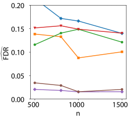
(a) Empirical FDR

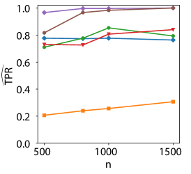
(b) Empirical TPR

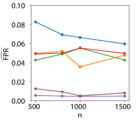
(c) Empirical FPR

Figure 4: Mean Shift Experiment: Rejection rates (estimated from 300 trials) for the six tests with $\alpha=0.05$ is shown.

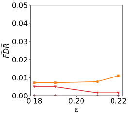
(a) Empirical FDR

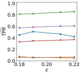
(b) Empirical TPR

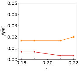
(c) Empirical FPR

Figure 5: RBM Experiment. Rejection rates (estimated from 300 trials) for the six tests with $\alpha=0.05$ is shown.

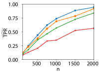
(a) $\widehat{\mathrm{TPR}}$ of $\widehat{\mathrm{MMD}}^{2}_{u}$

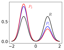
(b) Mixture Problem

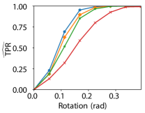
(c) $\widehat{\mathrm{TPR}}$ of $\widehat{\mathrm{KSD}}^{2}_{u}$

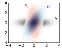
(d) Rotation Problem

Figure 6: $l=2$: The empirical true positive rate $\widehat{\mathrm{TPR}}$ of $\widehat{\mathrm{MMD}}^{2}_{u}$ (a) for the mixture problem of (b). We show empirical $\widehat{\mathrm{TPR}}$ of $\widehat{\mathrm{KSD}}^{2}_{u}$ (c) for rotation problem of (d). S:$a\%$ T:$b\%$ indicates that $a\%$ of the original dataset is used for selection and $b\%$ of the dataset used for testing.

H.2 TPR experiment

For this experiment, our goal is to empirically evaluate and validate Theorem 4.1 where $l=2$. For some sufficiently large $n$, it states that the TPR of RelPSI will be an upper bound for the TPR of RelMulti (for both MMD and KSD). We consider the following two synthetic problems:

1. Mixture of Gaussian: The candidate models and unknown distribution are $1$-d mixture of Gaussians where $M(\rho)=\rho\mathcal{N}(1,1)+(1-\rho)\mathcal{N}(-1,1)$ with mixing portion $\rho\in(0,1)$. We set the reference to be $R=M(0.5)$, and two candidate models to $P_{1}=M(0.7)$ and $P_{2}=M(0.75)$ (see Figure 6b). In this case, $P_{1}$ is closer to the reference distribution but only by a small amount. In this problem, we apply MMD and report the behaviour of the test as $n$ increases.

2. Rotating Gaussian: The two candidate models and our reference distributions are $2$-d Gaussian distributions that differ by rotation (see Figure 6d). We fix the sample size to $n=500$. Instead, we rotate the Gaussian distribution $P_{1}$ away from $P_{2}$ such that $P_{1}$ continues to get closer to the reference $R$ with each rotation. They are initially the same distribution but $P_{1}$ becomes a closer relative fit (with each rotation). In this problem, we apply KSD and report the empirical TPR as the Gaussian rotates and becomes an easier problem.

For each problem we consider three possible splits of the data: $25\%$, $50\%$, $25\%$ of the original samples for selection (and the rest for testing). Both problems use a Gaussian kernel with bandwidth set to $1$. The overall results are shown in Figure 6.

In Figure 6a, we plot the $\widehat{\mathrm{TPR}}$ for RelPSI-MMD and RelMulti-MMD for the Mixture of Gaussian problem. RelPSI performs the best with the highest empirical $\widehat{\mathrm{TPR}}$ confirming with Theorem 4.1. The next highest is RelMulti that performs a S:$25\%$ T:$75\%$ selection test split. The worst performer is the RelMulti with S:$75\%$ T:$25\%$ selection test split which can be explained by noting that most of the data has been used in selection, there is an insufficient amount of remaining data points to reject the hypothesis. The same behaviour can be observed in Figure 6c for $\widehat{\mathrm{KSD}}^{2}_{u}$. Overall, this experiment corroborates with our theoretical results that TPR of RelPSI will be higher in population.

References

- [1] Yoav Benjamini and Daniel Yekutieli. The control of the false discovery rate in multiple testing under dependency. The annals of statistics, 29(4):1165–1188, 2001.
- [2] A. Berlinet and C. Thomas-Agnan. Reproducing Kernel Hilbert Spaces in Probability and Statistics. Kluwer, 2004.
- [3] M. Bińkowski, D. J. Sutherland, M. Arbel, and A. Gretton. Demystifying MMD GANs. In ICLR. 2018.
- [4] Wacha Bounliphone, Eugene Belilovsky, Matthew B. Blaschko, Ioannis Antonoglou, and Arthur Gretton. A test of relative similarity for model selection in generative models. In International Conference on Learning Representations, 2016.
- [5] John Burkardt. The truncated normal distribution. Department of Scientific Computing Website, Florida State University, 2014.
- [6] Kacper Chwialkowski, Heiko Strathmann, and Arthur Gretton. A kernel test of goodness of fit. In International Conference on Machine Learning. PMLR, 2016.
- [7] Kacper P Chwialkowski, Aaditya Ramdas, Dino Sejdinovic, and Arthur Gretton. Fast two-sample testing with analytic representations of probability measures. In Advances in Neural Information Processing Systems, pages 1981–1989, 2015.
- [8] Moulines Eric, Francis R Bach, and Zaïd Harchaoui. Testing for homogeneity with kernel fisher discriminant analysis. In Advances in Neural Information Processing Systems, pages 609–616, 2008.
- [9] William Fithian, Dennis Sun, and Jonathan Taylor. Optimal inference after model selection. arXiv preprint arXiv:1410.2597, 2014.
- [10] Magalie Fromont, Matthieu Lerasle, Patricia Reynaud-Bouret, et al. Kernels based tests with non-asymptotic bootstrap approaches for two-sample problems. In Conference on Learning Theory, pages 23–1, 2012.
- [11] Kenji Fukumizu, Arthur Gretton, Xiaohai Sun, and Bernhard Schölkopf. Kernel measures of conditional dependence. In Advances in neural information processing systems, pages 489–496, 2008.
- [12] Mathieu Germain, Karol Gregor, Iain Murray, and Hugo Larochelle. MADE: Masked autoencoder for distribution estimation. In International Conference on Machine Learning, pages 881–889, 2015.
- [13] Jackson Gorham and Lester Mackey. Measuring sample quality with kernels. In Proceedings of the 34th International Conference on Machine Learning-Volume 70, pages 1292–1301. JMLR. org, 2017.
- [14] Arthur Gretton, Karsten M Borgwardt, Malte J Rasch, Bernhard Schölkopf, and Alexander Smola. A kernel two-sample test. Journal of Machine Learning Research, 13(Mar):723–773, 2012.
- [15] Arthur Gretton, Dino Sejdinovic, Heiko Strathmann, Sivaraman Balakrishnan, Massimiliano Pontil, Kenji Fukumizu, and Bharath K Sriperumbudur. Optimal kernel choice for large-scale two-sample tests. In Advances in neural information processing systems, pages 1205–1213, 2012.
- [16] Martin Heusel, Hubert Ramsauer, Thomas Unterthiner, Bernhard Nessler, and Sepp Hochreiter. GANs trained by a two time-scale update rule converge to a local nash equilibrium. In Advances in Neural Information Processing Systems, pages 6626–6637, 2017.
- [17] Wittawat Jitkrittum, Heishiro Kanagawa, Patsorn Sangkloy, James Hays, Bernhard Schölkopf, and Arthur Gretton. Informative features for model comparison. In Advances in Neural Information Processing Systems, 2018.
- [18] Wittawat Jitkrittum, Zoltán Szabó, Kacper P Chwialkowski, and Arthur Gretton. Interpretable distribution features with maximum testing power. In NIPS, pages 181–189. 2016.
- [19] Wittawat Jitkrittum, Wenkai Xu, Zoltán Szabó, Kenji Fukumizu, and Arthur Gretton. A linear-time kernel goodness-of-fit test. In Advances in Neural Information Processing Systems, pages 262–271, 2017.
- [20] Jason D Lee, Dennis L Sun, Yuekai Sun, and Jonathan E Taylor. Exact post-selection inference, with application to the Lasso. The Annals of Statistics, 44(3):907–927, 2016.
- [21] Hannes Leeb and Benedikt M Pötscher. Model selection and inference: Facts and fiction. Econometric Theory, 21(1):21–59, 2005.
- [22] Hannes Leeb, Benedikt M Pötscher, et al. Can one estimate the conditional distribution of post-model-selection estimators? The Annals of Statistics, 34(5):2554–2591, 2006.
- [23] Qiang Liu, Jason Lee, and Michael Jordan. A kernelized Stein discrepancy for goodness-of-fit tests. In International Conference on Machine Learning, pages 276–284, 2016.
- [24] Ziwei Liu, Ping Luo, Xiaogang Wang, and Xiaoou Tang. Large-scale celebfaces attributes (celeba) dataset. Retrieved August, 15:2018, 2018.
- [25] George Papamakarios, Theo Pavlakou, and Iain Murray. Masked autoregressive flow for density estimation. In Advances in Neural Information Processing Systems, pages 2338–2347, 2017.
- [26] Alex Smola, Arthur Gretton, Le Song, and Bernhard Schölkopf. A Hilbert space embedding for distributions. In International Conference on Algorithmic Learning Theory, pages 13–31. Springer, 2007.
- [27] Bharath K Sriperumbudur, Kenji Fukumizu, and Gert RG Lanckriet. Universality, characteristic kernels and rkhs embedding of measures. Journal of Machine Learning Research, 12(Jul):2389–2410, 2011.
- [28] Ingo Steinwart. On the influence of the kernel on the consistency of support vector machines. Journal of machine learning research, 2(Nov):67–93, 2001.
- [29] Shinya Suzumura, Kazuya Nakagawa, Yuta Umezu, Koji Tsuda, and Ichiro Takeuchi. Selective inference for sparse high-order interaction models. In Proceedings of the 34th International Conference on Machine Learning-Volume 70, pages 3338–3347. JMLR. org, 2017.
- [30] Christian Szegedy, Vincent Vanhoucke, Sergey Ioffe, Jon Shlens, and Zbigniew Wojna. Rethinking the inception architecture for computer vision. In Proceedings of the IEEE conference on computer vision and pattern recognition, pages 2818–2826, 2016.
- [31] Makoto Yamada, Denny Wu, Yao-Hung Hubert Tsai, Hirofumi Ohta, Ruslan Salakhutdinov, Ichiro Takeuchi, and Kenji Fukumizu. Post selection inference with incomplete maximum mean discrepancy estimator. In International Conference on Learning Representations, 2019.
- [32] Jiasen Yang, Qiang Liu, Vinayak Rao, and Jennifer Neville. Goodness-of-fit testing for discrete distributions via Stein discrepancy. In International Conference on Machine Learning, pages 5557–5566, 2018.
- [33] Wojciech Zaremba, Arthur Gretton, and Matthew Blaschko. B-test: A non-parametric, low variance kernel two-sample test. In Advances in neural information processing systems, pages 755–763, 2013.