Pulsar Timing Array Constraints on Primordial Black Holes with NANOGrav 11-Year Data Set

Abstract

The detection of binary black hole coalescences by LIGO/Virgo has aroused the interest in primordial black holes (PBHs), because they could be both the progenitors of these black holes and a compelling candidate of dark matter (DM). PBHs are formed soon after the enhanced scalar perturbations re-enter horizon during radiation dominated era, which would inevitably induce gravitational waves as well. Searching for such scalar induced gravitational waves (SIGWs) provides an elegant way to probe PBHs. We perform the first direct search for the signals of SIGWs accompanying the formation of PBHs in North American Nanohertz Observatory for Gravitational waves (NANOGrav) 11-year data set. No statistically significant detection has been made, and hence we place a stringent upper limit on the abundance of PBHs at $95\%$ confidence level. In particular, less than one part in a million of the total DM mass could come from PBHs in the mass range of $[2\times 10^{-3},7\times 10^{-1}]M_{\odot}$.

Introduction. Over the past few years, the great achievement of detecting gravitational waves (GWs) from binary black holes (BBHs) Abbott et al. (2016a, b, 2017a, 2017b, 2017c, c, 2018a) and a binary neutron star (BNS) Abbott et al. (2017d) by LIGO/Virgo has led us to the era of GW astronomy, as well as the era of multi-messenger astronomy. Various models have been proposed to account for the formation and evolution of these LIGO/Virgo BBHs, among which the PBH scenario Bird et al. (2016); Sasaki et al. (2016); Chen and Huang (2018) has attracted a lot of attention recently. PBHs are predicted to undergo gravitational collapse from overdensed regions in the infant universe Hawking (1971); Carr and Hawking (1974) when the corresponding wavelength of enhanced scalar curvature perturbations re-enter the horizon Ivanov et al. (1994); Yokoyama (1997); Garcia-Bellido et al. (1996); Ivanov (1998); Kawasaki et al. (2006).

The PBH scenario is appealing because it can not only account for the event rate of LIGO/Virgo BBHs, but also be a promising candidate for the long elusive missing part of our Universe – dark matter (DM). It is inconclusive that whether PBH can represent all DM or not, yet the abundance of PBHs ($f_{\mathrm{pbh}}$) which describes the total DM mass in the form of PBHs, has been constrained by a variety of observations, such as extra-galactic $\gamma$-rays from PBH evaporation Carr et al. (2010), femtolensing of $\gamma$-ray bursts Barnacka et al. (2012), Subaru/HSC microlensing Niikura et al. (2019a), Kepler milli/microlensing Griest et al. (2013), OGLE microlensing Niikura et al. (2019b), EROS/MACHO microlensing Tisserand et al. (2007), existence of white dwarfs (WDs) which are not triggered to explode in our local galaxy Graham et al. (2015) (this constraint might be ineffective according to the simulation in Montero-Camacho et al. (2019)), dynamical heating of ultra-faint dwarf galaxies Brandt (2016), X-ray/radio emission from the accretion of interstellar gas onto PBHs Gaggero et al. (2017), cosmic microwave background radiation from the accretion of primordial gas onto PBHs Ali-Haïmoud and Kamionkowski (2017); Aloni et al. (2017); Horowitz (2016); Chen et al. (2016), and GWs either through the null detection of sub-solar mass BBHs Abbott et al. (2018b); Magee et al. (2018); Chen and Huang (2019); Abbott et al. (2019) or the null detection of stochastic GW background (SGWB) from BBHs Wang et al. (2018); Chen and Huang (2019). But PBHs in a substantial window in the approximate mass range $[10^{-16},10^{-14}]\cup[10^{-13},10^{-12}]M_{\odot}$ are still allowed to account for all of the DM. We refer to Chen and Huang (2019) for a recent summary.

Actually there is another way to probe the PBH DM scenario, namely through the scalar induced GWs (SIGWs) which would inevitably be generated in conjunction with the formation of PBHs Tomita (1967); Saito and Yokoyama (2009); Young et al. (2014); Cai et al. (2019a); Yuan et al. (2019a); Cai et al. (2019b); Yuan et al. (2019b). The feature for distinguishing SIGW from other sources was sketched out in Yuan et al. (2019c) recently. Since PBHs are supposed to form from the tail of the probability density function of the curvature perturbations, the possibility to form a single PBH is quite sensitive to the amplitude of curvature perturbation power spectrum Young et al. (2014). Consequently the abundance of PBHs is extremely sensitive to the amplitude of the corresponding SIGW. Therefore a detection of SIGW will provide evidence for PBHs, while the null detection of SIGW will put a stringent constraint on the abundance of PBHs.

The peak frequency of the SIGW $(f_{*})$ is determined by the peak wave-mode of the comoving curvature power spectrum, and thus is related to the mass of PBHs by $f_{*}\sim 3\,{\rm{Hz}}\left({m_{\rm{pbh}}/10^{-18}M_{\odot}}\right)^{-1/2}$ Saito and Yokoyama (2009). The mass of PBHs constituting DM should be heavier than $10^{-18}M_{\odot}$, otherwise they would have evaporated due to Hawking radiation. As a result, the corresponding peak frequency of the SIGW should be lower than $3$Hz, and then it is difficult for the ground-based detectors like LIGO/Virgo to detect the corresponding SIGWs. On the other hand, the GW observatories hunting for low frequency signals are especially suitable to explore the PBH DM hypothesis, and the prospective constraints on the abundance of PBHs by LISA Audley et al. (2017) and pulsar timing observations such as IPTA Hobbs et al. (2010), FAST Nan et al. (2011) and SKA Kramer and Stappers (2015) have been investigated in Yuan et al. (2019a). See some other related works in Inomata et al. (2017); Schutz and Liu (2017); Orlofsky et al. (2017); Dror et al. (2019); Wang et al. (2019); Cai et al. (2019b); Clesse et al. (2018).

Despite the data of current pulsar timing array (PTA) has been used to constrain the amplitude of SGWBs, those results strongly depend on the assumption of some special power-law form which is quite different from SIGWs Yuan et al. (2019a). Therefore, in this article, we perform the first search in the public available PTA data set for the signal of SIGWs in order to test the PBH DM hypothesis. In particular, the null detection of SIGWs in the current NANOGrav 11-year data set Arzoumanian et al. (2018a) provides a constraint on the abundance of PBHs through SIGWs in the mass range of $[4\times 10^{-4},1.7]M_{\odot}$.

PBH DM and SIGW. In this article, we consider the monochromatic formation of PBHs, corresponding to a $\delta$ power spectrum of the scalar curvature perturbation, i.e.

$$\mathcal{P}_{\zeta}(f)=Af_{*}\delta\left(f-f_{*}\right),$$ (1)

where $A$ is the dimensionless amplitude of the power spectrum. In this case, the mass of the PBHs is related to the peak frequency $f_{*}$ by, Hawking (1971); Carr and Hawking (1974),

$${m_{\mathrm{pbh}}\over M_{\odot}}\simeq 2.3\times 10^{18}\left(\frac{H_{0}}{f_{*}}\right)^{2},$$ (2)

where $f_{*}$ is in units of Hz, and $H_{0}$ is the Hubble constant. The formation of PBH is a threshold process which is described by three-dimensional statistics of Gaussian random fields, also known as peak theory Bardeen et al. (1986), and the abundance of PBH in DM, $f_{\mathrm{pbh}}\equiv\Omega_{\mathrm{pbh}}/\Omega_{\mathrm{DM}}$, is given by, Carr et al. (2016),

$$f_{\mathrm{pbh}}\simeq 1.9\times 10^{7}\left({\zeta_{c}^{2}/A}-1\right)e^{-{\zeta_{c}^{2}\over 2A}}\left(\frac{m_{\mathrm{pbh}}}{M_{\odot}}\right)^{-\frac{1}{2}},$$ (3)

where $\zeta_{c}\simeq 1$ Musco et al. (2009, 2005); Musco and Miller (2013); Harada et al. (2013); Escrivà (2019); Escrivà et al. (2019) is the threshold value for the formation of PBHs.

In Maggiore (2000) the energy density of a GW background $\rho_{\mathrm{GW}}$ takes the form

$$\rho_{\mathrm{GW}}=\int\rho_{\mathrm{GW}}(f,\eta)\ \mathrm{d}\ln f={M_{p}^{2}\over 16a^{2}}\left\langle\overline{\partial_{k}h_{ij}\partial^{k}h^{ij}}\right\rangle,$$ (4)

where $\eta$ is the conformal time, $a$ is the scale factor, $M_{p}$ is the Planck mass, and the overline stands for time average. It is useful to introduce the dimensionless GW energy density parameter per logarithm frequency $\Omega_{\mathrm{GW}}(\eta,k)$ defined by

$$\Omega_{\mathrm{GW}}(\eta,f)\equiv\frac{\rho_{\mathrm{GW}}(f,\eta)}{\rho_{\rm{cr}}},$$ (5)

where $\rho_{\rm{cr}}$ is the critical energy of the present Universe. For a monochromatic formation of PBHs, the present $\Omega_{\mathrm{GW}}(f)$ of the SIGW in radiation dominated era can be estimated as Yuan et al. (2019a)

$$\Omega_{\mathrm{GW}}(f)=\Omega_{\mathrm{GW}}^{(2)}(f)+\Omega_{\mathrm{GW}}^{(3)}(f).$$ (6)

Here, the leading order contribution $\Omega_{\mathrm{GW}}^{(2)}(f)$ is given by, Espinosa et al. (2018); Kohri and Terada (2018),

$$\Omega_{\mathrm{GW}}^{(2)}(f) ={3\tilde{f}^{2}A^{2}\over 1024}\Omega_{r}(4-\tilde{f}^{2})^{2}(3\tilde{f}^{2}-2)^{2}\,\Theta(2-\tilde{f})\times$$ (7)

$$\qquad\Big{[}\pi^{2}(3\tilde{f}^{2}-2)^{2}\,\Theta(2\sqrt{3}-3\tilde{f})$$

$$\qquad\quad+\left(4+(3\tilde{f}^{2}-2)\log|1-\frac{4}{3\tilde{f}^{2}}|\right)^{2}\Big{]},$$

where $\tilde{f}\equiv f/f_{*}$ is the dimensionless frequency and $\Theta$ is the Heaviside theta function. In addition, the third-order correction $\Omega_{\mathrm{GW}}^{(3)}(f)$ reads, Yuan et al. (2019a),

$$\Omega_{\mathrm{GW}}^{(3)}(f)=\frac{A^{3}}{384\tilde{f}^{2}}\Omega_{r}\left(M_{2}\overline{I_{3}^{2}}+M_{1}\overline{I_{2}I_{4}}\right).$$ (8)

The definitions of $M_{1}$, $M_{2}$, $I_{2}$, $I_{3}$, and $I_{4}$ are complicated and can be found in Yuan et al. (2019a).

PTA data analysis. Null detection of certain GW backgrounds has been reported by the current PTAs such as NANOGrav, PPTA and EPTA, and the upper bounds on the amplitude of those GW backgrounds have also been continuing improved. For instance, NANOGrav constrained on the SGWB produced by supermassive black holes Aggarwal et al. (2018) and other spectra Arzoumanian et al. (2018b) such as power-law, broken-power-law, free and Gaussian-process ones. Similar studies were also performed by the PPTA collaboration Shannon et al. (2013) and the EPTA collaboration van Haasteren et al. (2011). In this article we search for the signal of SIGW using the NANOGrav 11-year data set which consists of time of arrival (TOA) data and pulsar timing models presented in Arzoumanian et al. (2018a). Similar to Kato and Soda (2019), we choose six pulsars which have relatively good TOA precision and long observation time. A summary of the basic properties of these pulsars is presented in Table 1. For all the $6$ pulsars, $T_{\rm{obs}}$ is longer than $8$ years, $N_{\rm{TOA}}$ is more than $10^{4}$, and RMS is less than $1.5\mu s$.

Table 1: Basic properties of the $6$ pulsars used in our analysis: RMS - the weighted root-mean-square epoch-averaged post-fit timing residuals, $N_{\rm{epoch}}$ - number of observational epochs, $N_{\rm{TOA}}$ - number of TOAs, $T_{\rm{obs}}$ - observational time span. See Ref. Arzoumanian et al. (2018a) in detail.

Pulsar name	RMS [$\mu$s]	$N_{\rm{epoch}}$	$N_{\rm{TOA}}$	$T_{\rm{obs}}$ [yr]
J0613$-$0200	0.422	324	11,566	10.8
J1012$+$5307	1.07	493	16,782	11.4
J1600$-$3053	0.23	275	12,433	8.1
J1713$+$0747	0.108	789	27,571	10.9
J1744$-$1134	0.842	322	11,550	11.4
J1909$-$3744	0.148	451	17,373	11.2

The presence of a GW background will manifest as the unexplained residuals in the TOAs of pulsar signals after subtracting a deterministic timing model that accounts for the pulsar spin behavior and the geometric effects due to the motion of the pulsar and the Earth Sazhin (1978); Detweiler (1979). It is therefore feasible to separate GW-induced residuals, which have distinctive correlations among different pulsars Hellings and Downs (1983), from other systematic effects, such as clock errors or delays due to light propagation through interstellar medium, by regularly monitoring TOAs of pulsars from an array of the most rotational stable millisecond pulsars Foster and Backer (1990). An $N_{\text{TOA}}$ length vector $\delta\bm{t}$ representing the timing residuals for a single pulsar can be modeled as follows Taylor et al. (2013); van Haasteren and Levin (2013)

$$\delta\bm{t}=\bm{M}\bm{\epsilon}+\delta\bm{t}_{\text{RGP}},$$ (9)

where $\bm{M}$ is the timing model design matrix, $\bm{\epsilon}$ is a vector denoting small offsets for the timing model parameters, and $\bm{M}\bm{\epsilon}$ is the residual due to inaccuracies of the timing model. The timing model design matrix is obtained through libstempo package which is a python interface to TEMPO2 Hobbs et al. (2006); Edwards et al. (2006) timing software. The term $\delta\bm{t}_{\text{RGP}}$ in Eq. (9) is the stochastic contribution to the TOAs, which can be modeled by a sum of random Gaussian processes van Haasteren and Vallisneri (2014) as

$$\delta\bm{t}_{\text{RGP}}=\delta\bm{t}_{\text{RN}}+\delta\bm{t}_{\text{WN}}+\delta\bm{t}_{\text{SSE}}+\delta\bm{t}_{\text{SIGW}}.$$ (10)

The first term on the right hand side of Eq. (10), $\delta\bm{t}_{\text{RN}}$, represents the red noise via a Fourier decomposition,

$$\delta\bm{t}_{\text{RN}}=\sum_{j=1}^{N_{\text{mode}}}\left[a_{j}\sin\left(\frac{2\pi jt}{T}\right)+b_{j}\cos\left(\frac{2\pi jt}{T}\right)\right]=\bm{F}\bm{a},$$ (11)

where ${N_{\text{mode}}}$ is the number of frequency modes included in the sum, $T$ is the total observation time span, $\bm{F}$ is the Fourier design matrix with components of alternating sine and cosine functions for frequencies in the range $[1/T,{N_{\text{mode}}}/T]$, and $\bm{a}$ is a vector giving the amplitude of the Fourier basis functions. In the analysis, we choose ${N_{\text{mode}}}=50$. The covariant matrix of the red noise coefficients $\bm{a}$ at frequency modes $i$ and $j$ will be diagonal, namely

$$\langle\bm{a}_{i}\bm{a}_{j}\rangle=P(f_{i})\,\delta_{ij},$$ (12)

where the power spectrum $P(f)$ is usually well described by a power-law model,

$$P(f)=\frac{A_{\rm{RN}}^{2}}{12\pi^{2}}\left(\frac{f}{\rm{yr}^{-1}}\right)^{3-\gamma_{\rm{RN}}}f^{-3},$$ (13)

with $A_{\rm{RN}}$ and $\gamma_{\rm{RN}}$ the amplitude and spectral index of the power-law, respectively. Note that in Eq. (12), $f_{i}$ is defined by $i/T$ if $i$ is odd, and $(i-1)/T$ if $i$ is even.

The second term, $\delta\bm{t}_{\text{WN}}$, accounts for the influence of white noise on the timing residuals, including a scale parameter on the TOA uncertainties (EFAC), an added variance (EQUAD) and a per-epoch variance (ECORR) for each backend/receiver system. This white noise is assumed to follow Gaussian distribution and can be characterized by a covariance matrix as

$$\bm{C}_{\text{WN}}=\bm{C}_{\text{EFAC}}+\bm{C}_{\text{EQUAD}}+\bm{C}_{\text{ECORR}},$$ (14)

where $\bm{C}_{\text{EFAC}}$, $\bm{C}_{\text{EQUAD}}$ and $\bm{C}_{\text{ECORR}}$ are the correlation functions for EFAC, EQUAD and ECORR parameters, respectively. Explicit expressions for these correlation functions can be found in Kato and Soda (2019).

The third term, $\delta\bm{t}_{\text{SSE}}$, is a noise due to inaccuracies of a solar system ephemeris (SSE) which is used to convert observatory TOAs to an inertial frame centered at the solar system barycenter. The SSE noise can seriously affect the upper limits and Bayes factors when searching for stochastic gravitational-wave backgrounds Arzoumanian et al. (2018b). In our analysis, we use DE436 Folkner and Park (2016) as the fiducial SSE model. To account for the SSE errors, we employ the physical model BayesEphem introduced in Arzoumanian et al. (2018b) and implemented in NANOGrav’s flagship package enterprise. The BayesEphem model has eleven parameters, including four parameters correspond to perturbations in the masses of the outer planets, one parameter describes a rotation rate about the ecliptic pole, and six parameters characterize the corrections to Earth’s orbit generated by perturbing Jupiter’s average orbital elements Arzoumanian et al. (2018b).

The last term, $\delta\bm{t}_{\text{SIGW}}$, is the observed timing residuals due to the SIGW, which are described by the cross-power spectral density Thrane and Romano (2013)

$$S_{IJ}(f)=\frac{H_{0}^{2}}{16\pi^{4}f^{5}}\Gamma_{IJ}(f)\ \Omega_{\mathrm{GW}}(f),$$ (15)

where $\Gamma_{IJ}$ is the Hellings & Downs coefficients Hellings and Downs (1983) measuring the spatial correlation of the pulsars $I$ and $J$ in the array. The expression for $\Omega_{\mathrm{GW}}(f)$ is given by Eq. (6). The free parameters for the SIGW are the amplitude $A$ and the peak frequency $f_{*}$. For a fixed $f_{*}$, the mass of PBH is given by Eq. (2). In this sense, the free parameter $A$ is directly related to the abundance of PBHs $f_{\rm{pbh}}$.

Table 2: Parameters and their prior distributions used in the analyses.

parameter	description	prior	comments
SIGW signal
$A$	GWB strain amplitude	Uniform $[10^{-5},10^{0}]$ (upper limits)
		log-Uniform $[-5,0]$ (model comparison)	one parameter for PTA
$f_{*}$	peak frequency	delta function	fixed
White Noise
$E_{k}$	EFAC per backend/receiver system	Uniform $[0,10]$	single-pulsar analysis only
$Q_{k}$[s]	EQUAD per backend/receiver system	log-Uniform $[-8.5,-5]$	single-pulsar analysis only
$J_{k}$[s]	ECORR per backend/receiver system	log-Uniform $[-8.5,-5]$	single-pulsar analysis only
Red Noise
$A_{\rm{RN}}$	red-noise power-law amplitude	Uniform $[10^{-20},10^{-11}]$ (upper limits)
		log-Uniform $[-20,-11]$ (model comparison)	one parameter per pulsar
$\gamma_{\rm{RN}}$	red-noise power-law spectral index	Uniform $[0,9]$	one parameter per pulsar
BayesEphem
$z_{\rm drift}$ [rad/yr]	drift-rate of Earth’s orbit about ecliptic $z$-axis	Uniform [$-10^{-9},10^{-9}$]	one parameter for PTA
$\Delta M_{\rm jupiter}$ [$M_{\odot}$]	perturbation to Jupiter’s mass	$\mathcal{N}(0,1.55\times 10^{-11})$	one parameter for PTA
$\Delta M_{\rm saturn}$ [$M_{\odot}$]	perturbation to Saturn’s mass	$\mathcal{N}(0,8.17\times 10^{-12})$	one parameter for PTA
$\Delta M_{\rm uranus}$ [$M_{\odot}$]	perturbation to Uranus’ mass	$\mathcal{N}(0,5.72\times 10^{-11})$	one parameter for PTA
$\Delta M_{\rm neptune}$ [$M_{\odot}$]	perturbation to Neptune’s mass	$\mathcal{N}(0,7.96\times 10^{-11})$	one parameter for PTA
PCAi	principal components of Jupiter’s orbit	Uniform $[-0.05,0.05]$	six parameters for PTA

For the timing model parameters and TOAs, we use the publicly available data files from NANOGrav 11-year data set Arzoumanian et al. (2018a). To extract information from the data, we perform a Bayesian inference by closely following the procedure in Arzoumanian et al. (2018b). The parameters of our model and their prior distributions are presented in Table 2. In order to reduce the computational costs, a common strategy is to fix the white noise parameters to their max likelihood values determined from independent single-pulsar analysis, in which only the white and red noises are considered. Fixing white noise parameters can greatly reduce the number of free parameters.

Assuming the $\delta\bm{t}_{\text{RGP}}$ is Gaussian and stationary, for a PTA with M pulsars, the likelihood function can be evaluated as, Ellis et al. (2013),

$$\mathcal{L}=\frac{1}{\sqrt{\det(2\pi\mathbf{\Sigma})}}\exp\left(-\frac{1}{2}\mathbf{R}^{T}\mathbf{\Sigma}^{-1}\mathbf{R}\right),$$ (16)

where $\mathbf{R}\equiv\left[\delta\bm{t}_{\text{RGP}}^{1},\delta\bm{t}_{\text{RGP}}^{2},\cdots,\delta\bm{t}_{\text{RGP}}^{M}\right]^{T}$ is a collection of $\delta\bm{t}_{\text{RGP}}$ for all pulsars, and $\mathbf{\Sigma}\equiv\langle\mathbf{R}\mathbf{R}^{T}\rangle$ is the covariance matrix. Following the common practice in Lentati et al. (2013); van Haasteren and Vallisneri (2014, 2015), we marginalize over the timing model parameter $\bm{\epsilon}$ when evaluating the likelihood. The likelihood is calculated by using the pulsar timing package enterprise. To achieve parallel tempering, we use PTMCMCSampler package to do the Markov chain Monte Carlo sampling.

Given the observational data $\mathcal{D}$, one needs to distinguish two exclusive models: a noise-only model $\mathcal{H}_{0}$ and a noise-plus-signal model $\mathcal{H}_{1}$. The model selection is quantified by the Bayes factor

$$B_{10}=\frac{\rm{evidence}[\mathcal{H}_{1}]}{\rm{evidence}[\mathcal{H}_{0}]}=\frac{p(A=0|\mathcal{H}_{1})}{p(A=0|\mathcal{D},\mathcal{H}_{1})},$$ (17)

where the numerator and denominator are the prior and posterior probability density of $A=0$ in the model $\mathcal{H}_{1}$, respectively. We have used the Savage-Dickey formula Dickey (1971) to estimate the Bayes factor in Eq. (17).

Results and conclusion. The upper limits and the Bayes factor for the power spectrum amplitude $A$ as a function of the peak frequency $f_{*}$ from the NANOGrav 11-year data set are showed in Fig. 1 at the $95\%$ confidence level. Even though there are two peaks in the Bayes factor distribution, both peak values are smaller than $3$, implying the presence of a signal in the data is “not worth more than a bare mention” Kass and Raftery (1995). Since the Bayes factor $B_{10}$ for each peak frequency is less than $3$, it indicates that the data is consistent with containing noise only. The upper limits on the abundance of PBHs in DM $f_{\mathrm{pbh}}$ as a function of the PBH mass $m_{\rm{pbh}}$ are given in Fig. 2 at the $95\%$ confidence level. Note that $m_{\rm{pbh}}$ is related to $f_{*}$ by Eq. (2), and $f_{\mathrm{pbh}}$ is related to $A$ and $m_{\rm{pbh}}$ by Eq. (3). Our results imply that the current PTA data set has already been able to place a stringent constraint on the abundance of PBHs through the SIGWs. According to Fig. 2, the abundance of PBHs is less than $10^{-6}$ in the mass range of $[2\times 10^{-3},7\times 10^{-1}]M_{\odot}$.

In this article, we give the first search for the signal of SIGWs inevitably accompanying the formation of PBHs in the NANOGrav 11-year data set. Since no significant signal is found, we place a $95\%$ upper limit on the amplitude of scalar perturbation over the peak frequency range of $[1.5\times 10^{-9},3\times 10^{-6}]$Hz and the abundance of PBHs in the mass range of $[4\times 10^{-4},1.7]M_{\odot}$. In particular, the abundance of PBHs in the mass range of $[2\times 10^{-3},7\times 10^{-1}]M_{\odot}$ less than $10^{-6}$, which is much better than any other observational constraints in this mass range in literature. Since the amplitude of SIGWs is roughly determined by the peak amplitude of scalar power spectrum even for the case with an extended mass distribution, a similar constraint on the peak amplitude of scalar power spectrum should be obtained from NANOGrav 11-yr data, and therefore a stringent constraint on the abundance of PBHs with an extended mass distribution can be also expected. In principle, the exact analysis for the case with an extended mass distribution is model-dependent, and will be left for the future.

Figure 1: Top panel: the $95\%$ upper limits on the power spectrum amplitude $A$ of curvature perturbation as a function of the peak frequency $f_{*}$ from the NANOGrav 11-year data set. Bottom panel: the corresponding Bayes factors $B_{10}$ as a function of the peak frequency $f_{*}$.

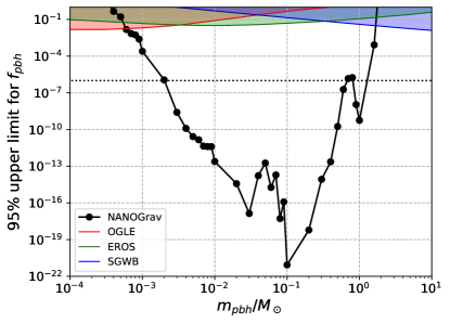
Figure 2: The $95\%$ upper limits on the abundance of PBHs in DM $f_{\mathrm{pbh}}$ as a function of the PBH mass $m_{\rm{pbh}}$ from the NANOGrav 11-year data set. Results from OGLE microlensing (OGLE) Niikura et al. (2019b), EROS/MACHO microlensing (EROS) Tisserand et al. (2007), and SGWB Chen and Huang (2019) are also shown. The horizontal dotted line corresponds to $10^{-6}$.

Acknowledgments. We acknowledge the use of HPC Cluster of ITP-CAS. This work is supported by grants from NSFC (grant No. 11975019, 11690021, 11991052, 11947302), the Strategic Priority Research Program of Chinese Academy of Sciences (Grant No. XDB23000000, XDA15020701), and Key Research Program of Frontier Sciences, CAS, Grant NO. ZDBS-LY-7009.

References

- Abbott et al. (2016a) B. P. Abbott et al. (LIGO Scientific, Virgo), “Observation of Gravitational Waves from a Binary Black Hole Merger,” Phys. Rev. Lett. 116, 061102 (2016a), arXiv:1602.03837 [gr-qc] .
- Abbott et al. (2016b) B. P. Abbott et al. (LIGO Scientific, Virgo), “GW151226: Observation of Gravitational Waves from a 22-Solar-Mass Binary Black Hole Coalescence,” Phys. Rev. Lett. 116, 241103 (2016b), arXiv:1606.04855 [gr-qc] .
- Abbott et al. (2017a) Benjamin P. Abbott et al. (LIGO Scientific, VIRGO), “GW170104: Observation of a 50-Solar-Mass Binary Black Hole Coalescence at Redshift 0.2,” Phys. Rev. Lett. 118, 221101 (2017a), [Erratum: Phys. Rev. Lett.121,no.12,129901(2018)], arXiv:1706.01812 [gr-qc] .
- Abbott et al. (2017b) B.. P.. Abbott et al. (LIGO Scientific, Virgo), “GW170608: Observation of a 19-solar-mass Binary Black Hole Coalescence,” Astrophys. J. 851, L35 (2017b), arXiv:1711.05578 [astro-ph.HE] .
- Abbott et al. (2017c) B. P. Abbott et al. (LIGO Scientific, Virgo), “GW170814: A Three-Detector Observation of Gravitational Waves from a Binary Black Hole Coalescence,” Phys. Rev. Lett. 119, 141101 (2017c), arXiv:1709.09660 [gr-qc] .
- Abbott et al. (2016c) B. P. Abbott et al. (LIGO Scientific, Virgo), “Binary Black Hole Mergers in the first Advanced LIGO Observing Run,” Phys. Rev. X6, 041015 (2016c), [erratum: Phys. Rev.X8,no.3,039903(2018)], arXiv:1606.04856 [gr-qc] .
- Abbott et al. (2018a) B. P. Abbott et al. (LIGO Scientific, Virgo), “GWTC-1: A Gravitational-Wave Transient Catalog of Compact Binary Mergers Observed by LIGO and Virgo during the First and Second Observing Runs,” (2018a), arXiv:1811.12907 [astro-ph.HE] .
- Abbott et al. (2017d) B. P. Abbott et al. (LIGO Scientific, Virgo), “GW170817: Observation of Gravitational Waves from a Binary Neutron Star Inspiral,” Phys. Rev. Lett. 119, 161101 (2017d), arXiv:1710.05832 [gr-qc] .
- Bird et al. (2016) Simeon Bird, Ilias Cholis, Julian B. Muñoz, Yacine Ali-Haïmoud, Marc Kamionkowski, Ely D. Kovetz, Alvise Raccanelli, and Adam G. Riess, “Did LIGO detect dark matter?” Phys. Rev. Lett. 116, 201301 (2016), arXiv:1603.00464 [astro-ph.CO] .
- Sasaki et al. (2016) Misao Sasaki, Teruaki Suyama, Takahiro Tanaka, and Shuichiro Yokoyama, “Primordial Black Hole Scenario for the Gravitational-Wave Event GW150914,” Phys. Rev. Lett. 117, 061101 (2016), [erratum: Phys. Rev. Lett.121,no.5,059901(2018)], arXiv:1603.08338 [astro-ph.CO] .
- Chen and Huang (2018) Zu-Cheng Chen and Qing-Guo Huang, “Merger Rate Distribution of Primordial-Black-Hole Binaries,” Astrophys. J. 864, 61 (2018), arXiv:1801.10327 [astro-ph.CO] .
- Hawking (1971) Stephen Hawking, “Gravitationally collapsed objects of very low mass,” Mon. Not. Roy. Astron. Soc. 152, 75 (1971).
- Carr and Hawking (1974) Bernard J. Carr and S. W. Hawking, “Black holes in the early Universe,” Mon. Not. Roy. Astron. Soc. 168, 399–415 (1974).
- Ivanov et al. (1994) P. Ivanov, P. Naselsky, and I. Novikov, “Inflation and primordial black holes as dark matter,” Phys. Rev. D50, 7173–7178 (1994).
- Yokoyama (1997) Junichi Yokoyama, “Formation of MACHO primordial black holes in inflationary cosmology,” Astron. Astrophys. 318, 673 (1997), arXiv:astro-ph/9509027 [astro-ph] .
- Garcia-Bellido et al. (1996) Juan Garcia-Bellido, Andrei D. Linde, and David Wands, “Density perturbations and black hole formation in hybrid inflation,” Phys. Rev. D54, 6040–6058 (1996), arXiv:astro-ph/9605094 [astro-ph] .
- Ivanov (1998) P. Ivanov, “Nonlinear metric perturbations and production of primordial black holes,” Phys. Rev. D57, 7145–7154 (1998), arXiv:astro-ph/9708224 [astro-ph] .
- Kawasaki et al. (2006) Masahiro Kawasaki, Tsutomu Takayama, Masahide Yamaguchi, and Jun’ichi Yokoyama, “Power Spectrum of the Density Perturbations From Smooth Hybrid New Inflation Model,” Phys. Rev. D74, 043525 (2006), arXiv:hep-ph/0605271 [hep-ph] .
- Carr et al. (2010) B. J. Carr, Kazunori Kohri, Yuuiti Sendouda, and Jun’ichi Yokoyama, “New cosmological constraints on primordial black holes,” Phys. Rev. D81, 104019 (2010), arXiv:0912.5297 [astro-ph.CO] .
- Barnacka et al. (2012) A. Barnacka, J. F. Glicenstein, and R. Moderski, “New constraints on primordial black holes abundance from femtolensing of gamma-ray bursts,” Phys. Rev. D86, 043001 (2012), arXiv:1204.2056 [astro-ph.CO] .
- Niikura et al. (2019a) Hiroko Niikura et al., “Microlensing constraints on primordial black holes with Subaru/HSC Andromeda observations,” Nat. Astron. 3, 524–534 (2019a), arXiv:1701.02151 [astro-ph.CO] .
- Griest et al. (2013) Kim Griest, Agnieszka M. Cieplak, and Matthew J. Lehner, “New Limits on Primordial Black Hole Dark Matter from an Analysis of Kepler Source Microlensing Data,” Phys. Rev. Lett. 111, 181302 (2013).
- Niikura et al. (2019b) Hiroko Niikura, Masahiro Takada, Shuichiro Yokoyama, Takahiro Sumi, and Shogo Masaki, “Constraints on Earth-mass primordial black holes from OGLE 5-year microlensing events,” Phys. Rev. D99, 083503 (2019b), arXiv:1901.07120 [astro-ph.CO] .
- Tisserand et al. (2007) P. Tisserand et al. (EROS-2), “Limits on the Macho Content of the Galactic Halo from the EROS-2 Survey of the Magellanic Clouds,” Astron. Astrophys. 469, 387–404 (2007), arXiv:astro-ph/0607207 [astro-ph] .
- Graham et al. (2015) Peter W. Graham, Surjeet Rajendran, and Jaime Varela, “Dark Matter Triggers of Supernovae,” Phys. Rev. D92, 063007 (2015), arXiv:1505.04444 [hep-ph] .
- Montero-Camacho et al. (2019) Paulo Montero-Camacho, Xiao Fang, Gabriel Vasquez, Makana Silva, and Christopher M. Hirata, “Revisiting constraints on asteroid-mass primordial black holes as dark matter candidates,” JCAP 1908, 031 (2019), arXiv:1906.05950 [astro-ph.CO] .
- Brandt (2016) Timothy D. Brandt, “Constraints on MACHO Dark Matter from Compact Stellar Systems in Ultra-Faint Dwarf Galaxies,” Astrophys. J. 824, L31 (2016), arXiv:1605.03665 [astro-ph.GA] .
- Gaggero et al. (2017) Daniele Gaggero, Gianfranco Bertone, Francesca Calore, Riley M. T. Connors, Mark Lovell, Sera Markoff, and Emma Storm, “Searching for Primordial Black Holes in the radio and X-ray sky,” Phys. Rev. Lett. 118, 241101 (2017), arXiv:1612.00457 [astro-ph.HE] .
- Ali-Haïmoud and Kamionkowski (2017) Yacine Ali-Haïmoud and Marc Kamionkowski, “Cosmic microwave background limits on accreting primordial black holes,” Phys. Rev. D95, 043534 (2017), arXiv:1612.05644 [astro-ph.CO] .
- Aloni et al. (2017) Daniel Aloni, Kfir Blum, and Raphael Flauger, “Cosmic microwave background constraints on primordial black hole dark matter,” JCAP 1705, 017 (2017), arXiv:1612.06811 [astro-ph.CO] .
- Horowitz (2016) Benjamin Horowitz, “Revisiting Primordial Black Holes Constraints from Ionization History,” (2016), arXiv:1612.07264 [astro-ph.CO] .
- Chen et al. (2016) Lu Chen, Qing-Guo Huang, and Ke Wang, “Constraint on the abundance of primordial black holes in dark matter from Planck data,” JCAP 1612, 044 (2016), arXiv:1608.02174 [astro-ph.CO] .
- Abbott et al. (2018b) B. P. Abbott et al. (LIGO Scientific, Virgo), “Search for Subsolar-Mass Ultracompact Binaries in Advanced LIGO’s First Observing Run,” Phys. Rev. Lett. 121, 231103 (2018b), arXiv:1808.04771 [astro-ph.CO] .
- Magee et al. (2018) Ryan Magee, Anne-Sylvie Deutsch, Phoebe McClincy, Chad Hanna, Christian Horst, Duncan Meacher, Cody Messick, Sarah Shandera, and Madeline Wade, “Methods for the detection of gravitational waves from subsolar mass ultracompact binaries,” Phys. Rev. D98, 103024 (2018), arXiv:1808.04772 [astro-ph.IM] .
- Chen and Huang (2019) Zu-Cheng Chen and Qing-Guo Huang, “Distinguishing Primordial Black Holes from Astrophysical Black Holes by Einstein Telescope and Cosmic Explorer,” (2019), arXiv:1904.02396 [astro-ph.CO] .
- Abbott et al. (2019) B. P. Abbott et al. (LIGO Scientific, Virgo), “Search for sub-solar mass ultracompact binaries in Advanced LIGO’s second observing run,” (2019), arXiv:1904.08976 [astro-ph.CO] .
- Wang et al. (2018) Sai Wang, Yi-Fan Wang, Qing-Guo Huang, and Tjonnie G. F. Li, “Constraints on the Primordial Black Hole Abundance from the First Advanced LIGO Observation Run Using the Stochastic Gravitational-Wave Background,” Phys. Rev. Lett. 120, 191102 (2018), arXiv:1610.08725 [astro-ph.CO] .
- Tomita (1967) Kenji Tomita, “Non-linear theory of gravitational instability in the expanding universe,” Progress of Theoretical Physics 37, 831–846 (1967).
- Saito and Yokoyama (2009) Ryo Saito and Jun’ichi Yokoyama, “Gravitational wave background as a probe of the primordial black hole abundance,” Phys. Rev. Lett. 102, 161101 (2009), [Erratum: Phys. Rev. Lett.107,069901(2011)], arXiv:0812.4339 [astro-ph] .
- Young et al. (2014) Sam Young, Christian T. Byrnes, and Misao Sasaki, “Calculating the mass fraction of primordial black holes,” JCAP 1407, 045 (2014), arXiv:1405.7023 [gr-qc] .
- Cai et al. (2019a) Rong-gen Cai, Shi Pi, and Misao Sasaki, “Gravitational Waves Induced by non-Gaussian Scalar Perturbations,” Phys. Rev. Lett. 122, 201101 (2019a), arXiv:1810.11000 [astro-ph.CO] .
- Yuan et al. (2019a) Chen Yuan, Zu-Cheng Chen, and Qing-Guo Huang, “Probing Primordial-Black-Hole Dark Matter with Scalar Induced Gravitational Waves,” (2019a), arXiv:1906.11549 [astro-ph.CO] .
- Cai et al. (2019b) Rong-Gen Cai, Shi Pi, Shao-Jiang Wang, and Xing-Yu Yang, “Pulsar Timing Array Constraints on the Induced Gravitational Waves,” (2019b), arXiv:1907.06372 [astro-ph.CO] .
- Yuan et al. (2019b) Chen Yuan, Zu-Cheng Chen, and Qing-Guo Huang, “Scalar Induced Gravitational Waves in Different Gauges,” (2019b), arXiv:1912.00885 [astro-ph.CO] .
- Yuan et al. (2019c) Chen Yuan, Zu-Cheng Chen, and Qing-Guo Huang, “Log-dependent slope of scalar induced gravitational waves in the infrared regions,” (2019c), arXiv:1910.09099 [astro-ph.CO] .
- Audley et al. (2017) Heather Audley et al. (LISA), “Laser Interferometer Space Antenna,” (2017), arXiv:1702.00786 [astro-ph.IM] .
- Hobbs et al. (2010) G. Hobbs et al., “The international pulsar timing array project: using pulsars as a gravitational wave detector,” Gravitational waves. Proceedings, 8th Edoardo Amaldi Conference, Amaldi 8, New York, USA, June 22-26, 2009, Class. Quant. Grav. 27, 084013 (2010), arXiv:0911.5206 [astro-ph.SR] .
- Nan et al. (2011) Rendong Nan, Di Li, Chengjin Jin, Qiming Wang, Lichun Zhu, Wenbai Zhu, Haiyan Zhang, Youling Yue, and Lei Qian, “The Five-Hundred-Meter Aperture Spherical Radio Telescope (FAST) Project,” Int. J. Mod. Phys. D20, 989–1024 (2011), arXiv:1105.3794 [astro-ph.IM] .
- Kramer and Stappers (2015) Michael Kramer and Ben Stappers, “Pulsar Science with the SKA,” Proceedings, Advancing Astrophysics with the Square Kilometre Array (AASKA14): Giardini Naxos, Italy, June 9-13, 2014, PoS AASKA14, 036 (2015).
- Inomata et al. (2017) Keisuke Inomata, Masahiro Kawasaki, Kyohei Mukaida, Yuichiro Tada, and Tsutomu T. Yanagida, “Inflationary primordial black holes for the LIGO gravitational wave events and pulsar timing array experiments,” Phys. Rev. D95, 123510 (2017), arXiv:1611.06130 [astro-ph.CO] .
- Schutz and Liu (2017) Katelin Schutz and Adrian Liu, “Pulsar timing can constrain primordial black holes in the LIGO mass window,” Phys. Rev. D95, 023002 (2017), arXiv:1610.04234 [astro-ph.CO] .
- Orlofsky et al. (2017) Nicholas Orlofsky, Aaron Pierce, and James D. Wells, “Inflationary theory and pulsar timing investigations of primordial black holes and gravitational waves,” Phys. Rev. D95, 063518 (2017), arXiv:1612.05279 [astro-ph.CO] .
- Dror et al. (2019) Jeff A. Dror, Harikrishnan Ramani, Tanner Trickle, and Kathryn M. Zurek, “Pulsar Timing Probes of Primordial Black Holes and Subhalos,” Phys. Rev. D100, 023003 (2019), arXiv:1901.04490 [astro-ph.CO] .
- Wang et al. (2019) Sai Wang, Takahiro Terada, and Kazunori Kohri, “Prospective constraints on the primordial black hole abundance from the stochastic gravitational-wave backgrounds produced by coalescing events and curvature perturbations,” Phys. Rev. D99, 103531 (2019), arXiv:1903.05924 [astro-ph.CO] .
- Clesse et al. (2018) Sebastien Clesse, Juan García-Bellido, and Stefano Orani, “Detecting the Stochastic Gravitational Wave Background from Primordial Black Hole Formation,” (2018), arXiv:1812.11011 [astro-ph.CO] .
- Arzoumanian et al. (2018a) Zaven Arzoumanian et al. (NANOGrav), “The NANOGrav 11-year Data Set: High-precision timing of 45 Millisecond Pulsars,” Astrophys. J. Suppl. 235, 37 (2018a), arXiv:1801.01837 [astro-ph.HE] .
- Bardeen et al. (1986) James M. Bardeen, J. R. Bond, Nick Kaiser, and A. S. Szalay, “The Statistics of Peaks of Gaussian Random Fields,” Astrophys. J. 304, 15–61 (1986).
- Carr et al. (2016) Bernard Carr, Florian Kuhnel, and Marit Sandstad, “Primordial Black Holes as Dark Matter,” Phys. Rev. D94, 083504 (2016), arXiv:1607.06077 [astro-ph.CO] .
- Musco et al. (2009) Ilia Musco, John C. Miller, and Alexander G. Polnarev, “Primordial black hole formation in the radiative era: Investigation of the critical nature of the collapse,” Class. Quant. Grav. 26, 235001 (2009), arXiv:0811.1452 [gr-qc] .
- Musco et al. (2005) Ilia Musco, John C. Miller, and Luciano Rezzolla, “Computations of primordial black hole formation,” Class. Quant. Grav. 22, 1405–1424 (2005), arXiv:gr-qc/0412063 [gr-qc] .
- Musco and Miller (2013) Ilia Musco and John C. Miller, “Primordial black hole formation in the early universe: critical behaviour and self-similarity,” Class. Quant. Grav. 30, 145009 (2013), arXiv:1201.2379 [gr-qc] .
- Harada et al. (2013) Tomohiro Harada, Chul-Moon Yoo, and Kazunori Kohri, “Threshold of primordial black hole formation,” Phys. Rev. D88, 084051 (2013), [Erratum: Phys. Rev.D89,no.2,029903(2014)], arXiv:1309.4201 [astro-ph.CO] .
- Escrivà (2019) Albert Escrivà, “Simulation of primordial black hole formation using pseudo-spectral methods,” (2019), arXiv:1907.13065 [gr-qc] .
- Escrivà et al. (2019) Albert Escrivà, Cristiano Germani, and Ravi K. Sheth, “A universal threshold for primordial black hole formation,” (2019), arXiv:1907.13311 [gr-qc] .
- Maggiore (2000) Michele Maggiore, “Gravitational wave experiments and early universe cosmology,” Phys. Rept. 331, 283–367 (2000), arXiv:gr-qc/9909001 [gr-qc] .
- Espinosa et al. (2018) José Ramón Espinosa, Davide Racco, and Antonio Riotto, “A Cosmological Signature of the SM Higgs Instability: Gravitational Waves,” JCAP 1809, 012 (2018), arXiv:1804.07732 [hep-ph] .
- Kohri and Terada (2018) Kazunori Kohri and Takahiro Terada, “Semianalytic calculation of gravitational wave spectrum nonlinearly induced from primordial curvature perturbations,” Phys. Rev. D97, 123532 (2018), arXiv:1804.08577 [gr-qc] .
- Aggarwal et al. (2018) K. Aggarwal et al., “The NANOGrav 11-Year Data Set: Limits on Gravitational Waves from Individual Supermassive Black Hole Binaries,” (2018), arXiv:1812.11585 [astro-ph.GA] .
- Arzoumanian et al. (2018b) Z. Arzoumanian et al. (NANOGRAV), “The NANOGrav 11-year Data Set: Pulsar-timing Constraints On The Stochastic Gravitational-wave Background,” Astrophys. J. 859, 47 (2018b), arXiv:1801.02617 [astro-ph.HE] .
- Shannon et al. (2013) R. M. Shannon et al., “Gravitational-wave Limits from Pulsar Timing Constrain Supermassive Black Hole Evolution,” Science 342, 334–337 (2013), arXiv:1310.4569 [astro-ph.CO] .
- van Haasteren et al. (2011) R. van Haasteren et al., “Placing limits on the stochastic gravitational-wave background using European Pulsar Timing Array data,” Mon. Not. Roy. Astron. Soc. 414, 3117–3128 (2011), [Erratum: Mon. Not. Roy. Astron. Soc.425,no.2,1597(2012)], arXiv:1103.0576 [astro-ph.CO] .
- Kato and Soda (2019) Ryo Kato and Jiro Soda, “Search for ultralight scalar dark matter with NANOGrav pulsar timing arrays,” (2019), arXiv:1904.09143 [astro-ph.HE] .
- Sazhin (1978) M. V. Sazhin, “Opportunities for detecting ultralong gravitational waves,” Soviet Astronomy 22, 36–38 (1978).
- Detweiler (1979) Steven L. Detweiler, “Pulsar timing measurements and the search for gravitational waves,” Astrophys. J. 234, 1100–1104 (1979).
- Hellings and Downs (1983) R. w. Hellings and G. s. Downs, “UPPER LIMITS ON THE ISOTROPIC GRAVITATIONAL RADIATION BACKGROUND FROM PULSAR TIMING ANALYSIS,” Astrophys. J. 265, L39–L42 (1983).
- Foster and Backer (1990) R. S. Foster and D. C. Backer, “Constructing a pulsar timing array,” Astrophys. J. 361, 300–308 (1990).
- Taylor et al. (2013) Stephen R. Taylor, Jonathan R. Gair, and L. Lentati, “Weighing The Evidence For A Gravitational-Wave Background In The First International Pulsar Timing Array Data Challenge,” Phys. Rev. D87, 044035 (2013), arXiv:1210.6014 [astro-ph.IM] .
- van Haasteren and Levin (2013) Rutger van Haasteren and Yuri Levin, “Understanding and analysing time-correlated stochastic signals in pulsar timing,” Mon. Not. Roy. Astron. Soc. 428, 1147 (2013), arXiv:1202.5932 [astro-ph.IM] .
- Hobbs et al. (2006) George Hobbs, R. Edwards, and R. Manchester, “Tempo2, a new pulsar timing package. 1. overview,” Mon. Not. Roy. Astron. Soc. 369, 655–672 (2006), arXiv:astro-ph/0603381 [astro-ph] .
- Edwards et al. (2006) Russell T. Edwards, G. B. Hobbs, and R. N. Manchester, “Tempo2, a new pulsar timing package. 2. The timing model and precision estimates,” Mon. Not. Roy. Astron. Soc. 372, 1549–1574 (2006), arXiv:astro-ph/0607664 [astro-ph] .
- van Haasteren and Vallisneri (2014) Rutger van Haasteren and Michele Vallisneri, “New advances in the Gaussian-process approach to pulsar-timing data analysis,” Phys. Rev. D90, 104012 (2014), arXiv:1407.1838 [gr-qc] .
- Folkner and Park (2016) William M. Folkner and Ryan S. Park, “JPL planetary and Lunar ephemeris DE436,” Jet Propulsion Laboratory (2016).
- Thrane and Romano (2013) Eric Thrane and Joseph D. Romano, “Sensitivity curves for searches for gravitational-wave backgrounds,” Phys. Rev. D88, 124032 (2013), arXiv:1310.5300 [astro-ph.IM] .
- Ellis et al. (2013) Justin A. Ellis, Xavier Siemens, and Rutger van Haasteren, “An Efficient Approximation to the Likelihood for Gravitational Wave Stochastic Background Detection Using Pulsar Timing Data,” Astrophys. J. 769, 63 (2013), arXiv:1302.1903 [astro-ph.IM] .
- Lentati et al. (2013) Lindley Lentati, P. Alexander, M. P. Hobson, S. Taylor, J. Gair, S. T. Balan, and R. van Haasteren, “Hyper-efficient model-independent Bayesian method for the analysis of pulsar timing data,” Phys. Rev. D87, 104021 (2013), arXiv:1210.3578 [astro-ph.IM] .
- van Haasteren and Vallisneri (2015) Rutger van Haasteren and Michele Vallisneri, “Low-rank approximations for large stationary covariance matrices, as used in the Bayesian and generalized-least-squares analysis…” Mon. Not. Roy. Astron. Soc. 446, 1170–1174 (2015), arXiv:1407.6710 [astro-ph.IM] .
- Dickey (1971) James M Dickey, “The weighted likelihood ratio, linear hypotheses on normal location parameters,” The Annals of Mathematical Statistics , 204–223 (1971).
- Kass and Raftery (1995) Robert E. Kass and Adrian E. Raftery, “Bayes factors,” Journal of the American Statistical Association 90, 773–795 (1995).