A Density-Based Basis-Set Incompleteness Correction for GW Methods

Abstract

Similar to other electron correlation methods, many-body perturbation theory methods based on Green functions, such as the so-called $GW$ approximation, suffer from the usual slow convergence of energetic properties with respect to the size of the one-electron basis set. This displeasing feature is due to the lack of explicit electron-electron terms modeling the infamous Kato electron-electron cusp and the correlation Coulomb hole around it. Here, we propose a computationally efficient density-based basis-set correction based on short-range correlation density functionals which significantly speeds up the convergence of energetics towards the complete basis set limit. The performance of this density-based correction is illustrated by computing the ionization potentials of the twenty smallest atoms and molecules of the GW100 test set at the perturbative $GW$ (or $G_{0}W_{0}$) level using increasingly large basis sets. We also compute the ionization potentials of the five canonical nucleobases (adenine, cytosine, thymine, guanine, and uracil) and show that, here again, a significant improvement is obtained.

I Introduction

The purpose of many-body perturbation theory (MBPT) based on Green functions is to solve the formidable many-body problem by adding the electron-electron Coulomb interaction perturbatively starting from an independent-particle model. Martin et al. (2016) In this approach, the screening of the Coulomb interaction is an essential quantity. Aryasetiawan and Gunnarsson (1998); Onida et al. (2002); Reining (2017)

The so-called $GW$ approximation is the workhorse of MBPT and has a long and successful history in the calculation of the electronic structure of solids. Aryasetiawan and Gunnarsson (1998); Onida et al. (2002); Reining (2017) $GW$ is getting increasingly popular in molecular systems Blase et al. (2011); Faber et al. (2011); Bruneval (2012); Bruneval et al. (2015, 2016); Bruneval (2016); Boulanger et al. (2014); Blase et al. (2016); Li et al. (2017); Hung et al. (2016, 2017); van Setten et al. (2015, 2018); Ou and Subotnik (2016, 2018); Faber (2014) thanks to efficient implementation relying on plane waves Marini et al. (2009); Deslippe et al. (2012); Maggio et al. (2017) or local basis functions. Blase et al. (2011, 2018); Bruneval et al. (2016); van Setten et al. (2013); Kaplan et al. (2015, 2016); Krause and Klopper (2017); Caruso et al. (2012, 2013, 2013); Caruso (2013) The $GW$ approximation stems from the acclaimed Hedin's equations Hedin (1965)

$$G(12)=G_{0}(12)+\int G_{0}(13)\Sigma(34)G(42)d(34),$$ (1a)

$$\Gamma(123)=\delta(12)\delta(13)$$

$$\qquad\qquad+\int\functionalderivative{\Sigma(12)}{G(45)}G(46)G(75)\Gamma(673)d(4567),$$ (1b)

$$P(12)=-i\int G(13)G(41)\Gamma(342)d(34),$$ (1c)

$$W(12)=\varv(12)+\int\varv(13)P(34)W(42)d(34),$$ (1d)

$$\Sigma(12)=i\int G(13)W(14)\Gamma(324)d(34),$$ (1e)

which connects the Green function $G$, its non-interacting version $G_{0}$, the irreducible vertex function $\Gamma$, the irreducible polarizability $P$, the dynamically-screened Coulomb interaction $W$ and the self-energy $\Sigma$, where $\varv$ is the bare Coulomb interaction, $\delta(12)$ is the Dirac delta function Olver et al. (2010) and $1$ is a composite coordinate gathering space, spin, and time variables $(\mathbf{r}_{1},\sigma_{1},t_{1})$. Within the $GW$ approximation, one bypasses the calculation of the vertex corrections by setting

$$\Gamma(123)\stackrel{{\scriptstyle GW}}{{\approx}}\delta(12)\delta(13).$$ (2)

Depending on the degree of self-consistency one is willing to perform, there exists several types of $GW$ calculations. Loos et al. (2018) The simplest and most popular variant of $GW$ is perturbative $GW$ (or $G_{0}W_{0}$). Hybertsen and Louie (1985, 1986) Although obviously starting-point dependent, Bruneval and Marques (2013); Jacquemin et al. (2016); Gui et al. (2018) it has been widely used in the literature to study solids, atoms, and molecules. Bruneval (2012); Bruneval and Marques (2013); van Setten et al. (2015, 2018) For finite systems such as atoms and molecules, partially Hybertsen and Louie (1986); Shishkin and Kresse (2007); Blase et al. (2011); Faber et al. (2011) or fully self-consistent Caruso et al. (2012, 2013, 2013); Caruso (2013) $GW$ methods have shown great promise. Ke (2011); Blase et al. (2011); Faber et al. (2011); Koval et al. (2014); Hung et al. (2016); Blase et al. (2018); Jacquemin et al. (2017)

Similar to other electron correlation methods, MBPT methods suffer from the usual slow convergence of energetic properties with respect to the size of the one-electron basis set. This can be tracked down to the lack of explicit electron-electron terms modeling the infamous electron-electron coalescence point (also known as Kato cusp Kato (1957)) and, more specifically, the Coulomb correlation hole around it. Pioneered by Hylleraas Hylleraas (1929) in the 1930's and popularized in the 1990's by Kutzelnigg and coworkers Kutzelnigg (1985); Noga and Kutzelnigg (1994); Kutzelnigg and Klopper (1991) (and subsequently others Kong et al. (2012); Hattig et al. (2012); Ten-no and Noga (2012); Ten-no (2012); Grüneis et al. (2017)), the so-called F12 methods overcome this slow convergence by employing geminal basis functions that closely resemble the correlation holes in electronic wave functions. F12 methods are now routinely employed in computational chemistry and provide robust tools for electronic structure calculations where small basis sets may be used to obtain near complete basis set (CBS) limit accuracy. Tew et al. (2007)

The basis-set correction presented here follow a different route, and relies on the range-separated density-functional theory (RS-DFT) formalism to capture, thanks to a short-range correlation functional, the missing part of the short-range correlation effects. Giner et al. (2018) As shown in recent studies on both ground- and excited-state properties, Loos et al. (2019); Giner et al. (2019) similar to F12 methods, it significantly speeds up the convergence of energetics towards the CBS limit while avoiding the usage of the large auxiliary basis sets that are used in F12 methods to avoid the numerous three- and four-electron integrals. Kong et al. (2012); Hattig et al. (2012); Ten-no and Noga (2012); Ten-no (2012); Grüneis et al. (2017); Barca et al. (2016); Barca and Loos (2017, 2018)

Explicitly correlated F12 correction schemes have been derived for second-order Green function methods (GF2) Szabo and Ostlund (1989); Casida and Chong (1989, 1991); Stefanucci and van Leeuwen (2013); Ortiz (2013); Phillips and Zgid (2014); Phillips et al. (2015); Rusakov et al. (2014); Rusakov and Zgid (2016); Hirata et al. (2015, 2017); Loos et al. (2018) by Ten-no and coworkers Ohnishi and Ten-no (2016); Johnson et al. (2018) and Valeev and coworkers. Pavošević et al. (2017); Teke et al. (2019) However, to the best of our knowledge, a F12-based correction for $GW$ has not been designed yet.

In the present manuscript, we illustrate the performance of the density-based basis-set correction developed in Refs. Giner et al., 2018; Loos et al., 2019; Giner et al., 2019 on ionization potentials obtained within $G_{0}W_{0}$. Note that the present basis-set correction can be straightforwardly applied to other properties (e.g, electron affinities and fundamental gaps), as well as other flavors of (self-consistent) $GW$ or Green function-based methods, such as GF2 (and its higher-order variants).

The paper is organized as follows. In Sec. II, we provide details about the theory behind the present basis-set correction and its adaptation to $GW$ methods. Results for a large collection of molecular systems are reported and discussed in Sec. IV. Finally, we draw our conclusions in Sec. V. Unless otherwise stated, atomic units are used throughout.

II Theory

II.1 MBPT with DFT basis-set correction

Following Ref. Giner et al., 2018, we start by defining, for a $N$-electron system with nuclei-electron potential $v_{\text{ne}}(\mathbf{r})$, the approximate ground-state energy for one-electron densities $n$ which are ``representable'' in a finite basis set $\mathcal{B}$

$$E_{0}^{\mathcal{B}}=\min_{n\in\mathcal{D}^{\mathcal{B}}}\quantity{F[n]+\int v_{\text{ne}}(\mathbf{r})n(\mathbf{r})d\mathbf{r}},$$ (3)

where $\mathcal{D}^{\mathcal{B}}$ is the set of $N$-representable densities which can be extracted from a wave function $\Psi^{\mathcal{B}}$ expandable in the Hilbert space generated by $\mathcal{B}$. In this expression,

$$F[n]=\min_{\Psi\rightsquigarrow n}\matrixelement*{\Psi}{\hat{T}+\hat{W}_{\text{ee}}}{\Psi}$$ (4)

is the exact Levy-Lieb universal density functional, Levy (1979, 1982); Lieb (1983) where the notation $\Psi\rightsquigarrow n$ in Eq. (3) states that $\Psi$ yields the one-electron density $n$. $\hat{T}$ and $\hat{W}_{\text{ee}}$ are the kinetic and electron-electron interaction operators. The exact Levy-Lieb universal density functional is then decomposed as

$$F[n]=F^{\mathcal{B}}[n]+\bar{E}^{\mathcal{B}}[n],$$ (5)

where $F^{\mathcal{B}}[n]$ is the Levy-Lieb density functional with wave functions $\Psi^{\mathcal{B}}$ expandable in the Hilbert space generated by $\mathcal{B}$

$$F^{\mathcal{B}}[n]=\min_{\Psi^{\mathcal{B}}\rightsquigarrow n}\matrixelement*{\Psi^{\mathcal{B}}}{\hat{T}+\hat{W}_{\text{ee}}}{\Psi^{\mathcal{B}}},$$ (6)

and $\bar{E}^{\mathcal{B}}[n]$ is the complementary basis-correction density functional. Giner et al. (2018) In the present work, instead of using wave-function methods for calculating $F^{\mathcal{B}}[n]$, we use Green-function methods. We assume that there exists a functional $\Omega^{\mathcal{B}}[G^{\mathcal{B}}]$ of $N$-representable one-electron Green functions $G^{\mathcal{B}}(\mathbf{r},\mathbf{r}^{\prime},\omega)$ representable in the basis set $\mathcal{B}$ and yielding the density $n$ which gives $F^{\mathcal{B}}[n]$ at a stationary point

$$F^{\mathcal{B}}[n]=\underset{G^{\mathcal{B}}\rightsquigarrow n}{\text{stat}}\Omega^{\mathcal{B}}[G^{\mathcal{B}}].$$ (7)

The reason why we use a stationary condition rather than a minimization condition is that only a stationary property is generally known for functionals of the Green function. For example, we can choose for $\Omega^{\mathcal{B}}[G]$ a Klein-like energy functional (see, e.g, Refs. Stefanucci and van Leeuwen, 2013; Martin et al., 2016; Dahlen and van Leeuwen, 2005; Dahlen et al., 2005, 2006)

$$\Omega^{\mathcal{B}}[G]=\Tr[\ln(-G)]-\Tr[(G_{\text{f}}^{\mathcal{B}})^{-1}G-1]+\Phi_{\text{Hxc}}^{\mathcal{B}}[G],$$ (8)

where $(G_{\text{f}}^{\mathcal{B}})^{-1}$ is the projection into $\mathcal{B}$ of the inverse free-particle Green function

$$(G_{\text{f}})^{-1}(\mathbf{r},\mathbf{r}^{\prime},\omega)=\quantity(\omega+\frac{\nabla^{2}_{\mathbf{r}}}{2})\delta(\mathbf{r}-\mathbf{r}^{\prime}),$$ (9)

and we have introduced the trace

$$\Tr[AB]=\int_{-\infty}^{+\infty}\frac{d\omega}{2\pi i}e^{i\omega 0^{+}}\iint A(\mathbf{r},\mathbf{r}^{\prime},\omega)B(\mathbf{r}^{\prime},\mathbf{r}{},\omega)d\mathbf{r}d\mathbf{r}^{\prime}.$$ (10)

In Eq. (8), $\Phi_{\text{Hxc}}^{\mathcal{B}}[G]$ is a Hartree-exchange-correlation (Hxc) functional of the Green function such that its functional derivatives yields the Hxc self-energy in the basis

$$\functionalderivative{\Phi_{\text{Hxc}}^{\mathcal{B}}[G]}{G(\mathbf{r},\mathbf{r}^{\prime},\omega)}=\Sigma_{\text{Hxc}}^{\mathcal{B}}[G](\mathbf{r},\mathbf{r}^{\prime},\omega).$$ (11)

Inserting Eqs. (5) and (7) into Eq. (3), we finally arrive at

$$E_{0}^{\mathcal{B}}=\underset{G^{\mathcal{B}}}{\text{stat}}\quantity{\Omega^{\mathcal{B}}[G^{\mathcal{B}}]+\int v_{\text{ne}}(\mathbf{r})n_{G^{\mathcal{B}}}(\mathbf{r})d\mathbf{r}+\bar{E}^{\mathcal{B}}[n_{G^{\mathcal{B}}}]},$$ (12)

where the stationary point is searched over $N$-representable one-electron Green functions $G^{\mathcal{B}}(\mathbf{r},\mathbf{r}^{\prime},\omega)$ representable in the basis set $\mathcal{B}$.

The stationary condition from Eq. (12) is

$$\functionalderivative{G^{\mathcal{B}}}\Bigg{(}\Omega^{\mathcal{B}}[G^{\mathcal{B}}]+\int v_{\text{ne}}(\mathbf{r})n_{G^{\mathcal{B}}}(\mathbf{r})d\mathbf{r}+\bar{E}^{\mathcal{B}}[n_{G^{\mathcal{B}}}]\\ -\lambda\int n_{G^{\mathcal{B}}}(\mathbf{r})d\mathbf{r}\Bigg{)}=0,$$ (13)

where $\lambda$ is the chemical potential (enforcing the electron number). It leads the following Dyson equation

$$(G^{\mathcal{B}})^{-1}=(G_{0}^{\mathcal{B}})^{-1}-\Sigma_{\text{Hxc}}^{\mathcal{B}}[G^{\mathcal{B}}]-\bar{\Sigma}^{\mathcal{B}}[n_{G^{\mathcal{B}}}],$$ (14)

where $(G_{0}^{\mathcal{B}})^{-1}$ is the basis projection of the inverse non-interacting Green function with potential $v_{\text{ne}}(\mathbf{r})$, i.e,

$$(G_{0})^{-1}(\mathbf{r},\mathbf{r}^{\prime},\omega)=\quantity(\omega+\frac{\nabla_{\mathbf{r}}^{2}}{2}-v_{\text{ne}}(\mathbf{r})+\lambda)\delta(\mathbf{r}-\mathbf{r}^{\prime}),$$ (15)

and $\bar{\Sigma}^{\mathcal{B}}$ is a frequency-independent local self-energy coming from the functional derivative of the complementary basis-correction density functional

$$\bar{\Sigma}^{\mathcal{B}}[n](\mathbf{r},\mathbf{r}^{\prime})=\bar{v}^{\mathcal{B}}[n](\mathbf{r})\delta(\mathbf{r}-\mathbf{r}^{\prime}),$$ (16)

with $\bar{v}^{\mathcal{B}}[n](\mathbf{r})=\delta\bar{E}^{\mathcal{B}}[n]/\delta n(\mathbf{r})$. This is found from Eq. (13) by using the chain rule,

$$\functionalderivative{\bar{E}^{\mathcal{B}}[n]}{G(\mathbf{r},\mathbf{r}^{\prime},\omega)}=\int\functionalderivative{\bar{E}^{\mathcal{B}}[n]}{n(\mathbf{r}^{\prime\prime})}\functionalderivative{n(\mathbf{r}^{\prime\prime})}{G(\mathbf{r},\mathbf{r}^{\prime},\omega)}d\mathbf{r}^{\prime\prime},$$ (17)

and

$$n(\mathbf{r})=\int_{-\infty}^{+\infty}\frac{d\omega}{2\pi i}e^{i\omega 0^{+}}G(\mathbf{r},\mathbf{r},\omega).$$ (18)

The solution of the Dyson equation (14) gives the Green function $G^{\mathcal{B}}(\mathbf{r},\mathbf{r}^{\prime},\omega)$ which is not exact (even using the exact complementary basis-correction density functional $\bar{\Sigma}^{\mathcal{B}}[n]$) but should converge more rapidly with the basis set thanks to the presence of the basis-set correction $\bar{\Sigma}^{\mathcal{B}}$. Of course, in the CBS limit, the basis-set correction vanishes and the Green function becomes exact, i.e,

$$\lim_{\mathcal{B}\to\text{CBS}}\bar{\Sigma}^{\mathcal{B}} =0, \lim_{\mathcal{B}\to\text{CBS}}G^{\mathcal{B}} =G.$$ (19)

The Dyson equation (14) can also be written with an arbitrary reference

$$(G^{\mathcal{B}})^{-1}=(G_{\text{ref}}^{\mathcal{B}})^{-1}-\quantity(\Sigma_{\text{Hxc}}^{\mathcal{B}}[G^{\mathcal{B}}]-\Sigma_{\text{ref}}^{\mathcal{B}})-\bar{\Sigma}^{\mathcal{B}}[n_{G^{\mathcal{B}}}],$$ (20)

where $(G_{\text{ref}}^{\mathcal{B}})^{-1}=(G_{0}^{\mathcal{B}})^{-1}-\Sigma_{\text{ref}}^{\mathcal{B}}$. For example, if the reference is Hartree-Fock (HF), $\Sigma_{\text{ref}}^{\mathcal{B}}(\mathbf{r},\mathbf{r}^{\prime})=\Sigma_{\text{Hx}}^{\mathcal{B}}(\mathbf{r},\mathbf{r}^{\prime})$ is the HF nonlocal self-energy, and if the reference is Kohn-Sham (KS), $\Sigma_{\text{ref}}^{\mathcal{B}}(\mathbf{r},\mathbf{r}^{\prime})=v_{\text{Hxc}}^{\mathcal{B}}(\mathbf{r})\delta(\mathbf{r}-\mathbf{r}^{\prime})$ is the local Hxc potential.

Note that the present basis-set correction is applicable to any approximation of the self-energy (irrespectively of the diagrams included) without altering the CBS limit of such methods. Consequently, it can be applied, for example, to GF2 methods (also known as second Born approximation Stefanucci and van Leeuwen (2013) in the condensed-matter community) or higher orders. Szabo and Ostlund (1989); Casida and Chong (1989, 1991); Stefanucci and van Leeuwen (2013); Ortiz (2013); Phillips and Zgid (2014); Phillips et al. (2015); Rusakov et al. (2014); Rusakov and Zgid (2016); Hirata et al. (2015, 2017); Loos et al. (2018) Note, however, that the basis-set correction is optimal for the exact self-energy within a given basis set, since it corrects only for the basis-set error and not for the chosen approximate form of the self-energy within the basis set.

II.2 The $GW$ Approximation

In this subsection, we provide the minimal set of equations required to describe $G_{0}W_{0}$. More details can be found, for example, in Refs. 25; 27; 9. For the sake of simplicity, we only give the equations for closed-shell systems with a KS single-particle reference (with a local potential). The one-electron energies $\epsilon_{p}$ and their corresponding (real-valued) orbitals $\phi_{p}(\mathbf{r})$ (which defines the basis set $\mathcal{B}$) are then the KS orbitals and their orbital energies.

Within the $GW$ approximation, the correlation part of the self-energy reads

$$\begin{split}\Sigma_{\text{c},p}^{\mathcal{B}}(\omega)&=\matrixelement*{\phi_{p}}{\Sigma_{\text{c}}^{\mathcal{B}}(\omega)}{\phi_{p}}\\ &=2\sum_{i}^{N_{\text{occ}}}\sum_{m}\frac{[pi|m]^{2}}{\omega-\epsilon_{i}+\Omega_{m}-i\eta}\\ &+2\sum_{a}^{N_{\text{virt}}}\sum_{m}\frac{[pa|m]^{2}}{\omega-\epsilon_{a}-\Omega_{m}+i\eta},\end{split}$$ (21)

where $i$ runs over the $N_{\text{occ}}$ occupied orbitals, $a$ runs over the $N_{\text{virt}}$ virtual orbitals, $m$ labels excited states (see below), and $\eta$ is a positive infinitesimal. The screened two-electron integrals

$$[pq|m]=\sum_{i}^{N_{\text{occ}}}\sum_{a}^{N_{\text{virt}}}(pq|ia)(\boldsymbol{X}_{m}+\boldsymbol{Y}_{m})_{ia}$$ (22)

are obtained via the contraction of the bare two-electron integrals Gill (1994)

$$(pq|rs)=\iint\frac{\phi_{p}(\mathbf{r})\phi_{q}(\mathbf{r})\phi_{r}(\mathbf{r}^{\prime})\phi_{s}(\mathbf{r}^{\prime})}{\absolutevalue*{\mathbf{r}-\mathbf{r}^{\prime}}}d\mathbf{r}d\mathbf{r}^{\prime},$$ (23)

and the transition densities $(\boldsymbol{X}_{m}+\boldsymbol{Y}_{m})_{ia}$ originating from a (direct) random-phase approximation (RPA) calculation Casida (1995); Dreuw and Head-Gordon (2005)

$$\begin{pmatrix}\boldsymbol{A}&\boldsymbol{B}\\ -\boldsymbol{B}&-\boldsymbol{A}\\ \end{pmatrix}\begin{pmatrix}\boldsymbol{X}_{m}\\ \boldsymbol{Y}_{m}\\ \end{pmatrix}=\Omega_{m}\begin{pmatrix}\boldsymbol{X}_{m}\\ \boldsymbol{Y}_{m}\\ \end{pmatrix},$$ (24)

with

$$A_{ia,jb} =\delta_{ij}\delta_{ab}(\epsilon_{a}-\epsilon_{i})+2(ia|bj), B_{ia,jb} =2(ia|jb),$$ (25)

and $\delta_{pq}$ is the Kronecker delta. Olver et al. (2010) Equation (24) also provides the RPA neutral excitation energies $\Omega_{m}$ which correspond to the poles of the screened Coulomb interaction $W(\omega)$.

The $G_{0}W_{0}$ quasiparticle energies $\epsilon^{\text{$G_{0}W_{0}$}}_{p}$ are provided by the solution of the (non-linear) quasiparticle equation Hybertsen and Louie (1985); van Setten et al. (2013); Veril et al. (2018)

$$\omega=\epsilon_{p}-V_{\text{xc},p}^{\mathcal{B}}+\Sigma_{\text{x},p}^{\mathcal{B}}+\real[\Sigma_{\text{c},p}^{\mathcal{B}}(\omega)].$$ (26)

with the largest renormalization weight (or factor)

$$Z_{p}=\quantity[1-\left.\partialderivative{\real[\Sigma_{\text{c},p}^{\mathcal{B}}(\omega)]}{\omega}\right|_{\omega=\epsilon_{p}}]^{-1}.$$ (27)

Because of sum rules, Martin and Schwinger (1959); Baym and Kadanoff (1961); Baym (1962); von Barth and Holm (1996) the other solutions, known as satellites, share the remaining weight. In Eq. (26), $\Sigma_{\text{x},p}^{\mathcal{B}}=\matrixelement*{\phi_{p}}{\Sigma_{\text{x}}^{\mathcal{B}}}{\phi_{p}}$ is the (static) HF exchange part of the self-energy and

$$V_{\text{xc},p}^{\mathcal{B}}=\int\phi_{p}(\mathbf{r})v_{\text{xc}}^{\mathcal{B}}(\mathbf{r})\phi_{p}(\mathbf{r})d\mathbf{r},$$ (28)

where $v_{\text{xc}}^{\mathcal{B}}(\mathbf{r})$ is the KS exchange-correlation potential. In particular, the ionization potential (IP) and electron affinity (EA) are extracted thanks to the following relationships: Szabo and Ostlund (1989)

IP $$=-\epsilon^{\text{$G_{0}W_{0}$}}_{\text{HOMO}}, =-\epsilon^{\text{$G_{0}W_{0}$}}_{\text{LUMO}},$$ EA (29)

where $\epsilon^{\text{$G_{0}W_{0}$}}_{\text{HOMO}}$ and $\epsilon^{\text{$G_{0}W_{0}$}}_{\text{LUMO}}$ are the HOMO and LUMO quasiparticle energies, respectively.

II.3 Basis-set correction

The fundamental idea behind the present basis-set correction is to recognize that the singular two-electron Coulomb interaction $\absolutevalue*{\mathbf{r}-\mathbf{r}^{\prime}}^{-1}$ projected in a finite basis $\mathcal{B}$ is a finite, non-divergent quantity at $\absolutevalue*{\mathbf{r}-\mathbf{r}^{\prime}}=0$, which ``resembles'' the long-range interaction operator $\absolutevalue*{\mathbf{r}-\mathbf{r}^{\prime}}^{-1}\erf(\mu\absolutevalue*{\mathbf{r}-\mathbf{r}^{\prime}})$ used within RS-DFT. Giner et al. (2018)

We start therefore by considering an effective non-divergent two-electron interaction $W^{\mathcal{B}}(\mathbf{r},\mathbf{r}^{\prime})$ within the basis set which reproduces the expectation value of the Coulomb interaction over a given pair density $n_{2}^{\mathcal{B}}(\mathbf{r},\mathbf{r}^{\prime})$, i.e,

$$\frac{1}{2}\iint\frac{n_{2}^{\mathcal{B}}(\mathbf{r},\mathbf{r}^{\prime})}{\absolutevalue*{\mathbf{r}-\mathbf{r}^{\prime}}}d\mathbf{r}d\mathbf{r}^{\prime}=\frac{1}{2}\iint n_{2}^{\mathcal{B}}(\mathbf{r},\mathbf{r}^{\prime})W^{\mathcal{B}}(\mathbf{r},\mathbf{r}^{\prime})d\mathbf{r}d\mathbf{r}^{\prime}.$$ (30)

The properties of $W^{\mathcal{B}}(\mathbf{r},\mathbf{r}^{\prime})$ are detailed in Ref. Giner et al., 2018. A key aspect is that because the value of $W^{\mathcal{B}}(\mathbf{r},\mathbf{r}^{\prime})$ at coalescence, $W^{\mathcal{B}}(\mathbf{r},\mathbf{r})$, is necessarily finite in a finite basis $\mathcal{B}$, one can approximate $W^{\mathcal{B}}(\mathbf{r},\mathbf{r}^{\prime})$ by a non-divergent, long-range interaction of the form

$$W^{\mathcal{B}}(\mathbf{r},\mathbf{r}^{\prime})\approx\frac{1}{2}\quantity{\frac{\erf[\mu^{\mathcal{B}}(\mathbf{r})\absolutevalue*{\mathbf{r}-\mathbf{r}^{\prime}}]}{\absolutevalue*{\mathbf{r}-\mathbf{r}^{\prime}}}+\frac{\erf[\mu^{\mathcal{B}}(\mathbf{r}^{\prime})\absolutevalue*{\mathbf{r}-\mathbf{r}^{\prime}}]}{\absolutevalue*{\mathbf{r}-\mathbf{r}^{\prime}}}}.$$ (31)

The information about the finiteness of the basis set is then transferred to the range-separation function $\mu^{\mathcal{B}}(\mathbf{r})$, and its value can be determined by ensuring that the two sides of Eq. (31) are strictly equal at $\absolutevalue*{\mathbf{r}-\mathbf{r}^{\prime}}=0$. Knowing that $\lim_{r\to 0}\erf(\mu r)/r=2\mu/\sqrt{\pi}$, this yields

$$\mu^{\mathcal{B}}(\mathbf{r})=\frac{\sqrt{\pi}}{2}W^{\mathcal{B}}(\mathbf{r},\mathbf{r}).$$ (32)

Following Refs. Giner et al., 2018; Loos et al., 2019; Giner et al., 2019, we adopt the following definition for $W^{\mathcal{B}}(\mathbf{r},\mathbf{r}^{\prime})$

$$W^{\mathcal{B}}(\mathbf{r},\mathbf{r}^{\prime})=\begin{cases}f^{\mathcal{B}}(\mathbf{r},\mathbf{r}^{\prime})/n_{2}^{\mathcal{B}}(\mathbf{r},\mathbf{r}^{\prime}),&\text{if }n_{2}^{\mathcal{B}}(\mathbf{r},\mathbf{r}^{\prime})\neq 0,\\ \infty,&\text{otherwise},\\ \end{cases}$$ (33)

where, in this work, $f^{\mathcal{B}}(\mathbf{r},\mathbf{r}^{\prime})$ and $n_{2}^{\mathcal{B}}(\mathbf{r},\mathbf{r}^{\prime})$ are calculated using the opposite-spin two-electron density matrix of a spin-restricted single determinant (such as HF and KS). For a closed-shell system, we have

$$f^{\mathcal{B}}(\mathbf{r},\mathbf{r}^{\prime})=2\sum_{pq}^{N_{\text{bas}}}\sum_{ij}^{N_{\text{occ}}}\phi_{p}(\mathbf{r})\phi_{i}(\mathbf{r})(pi|qj)\phi_{q}(\mathbf{r}^{\prime})\phi_{j}(\mathbf{r}^{\prime}),$$ (34)

and

$$n_{2}^{\mathcal{B}}(\mathbf{r},\mathbf{r}^{\prime}) = 2\sum_{ij}^{N_{\text{occ}}}\phi_{i}(\mathbf{r})^{2}\phi_{j}(\mathbf{r}^{\prime})^{2}=\frac{1}{2}n^{\mathcal{B}}(\mathbf{r})n^{\mathcal{B}}(\mathbf{r}^{\prime}),$$ (35)

where $n^{\mathcal{B}}(\mathbf{r})$ is the one-electron density. The quantity $n_{2}^{\mathcal{B}}(\mathbf{r},\mathbf{r}^{\prime})$ represents the opposite-spin pair density of a closed-shell system with a single-determinant wave function. Note that in Eq. (34) the indices $p$ and $q$ run over all occupied and virtual orbitals ($N_{\text{bas}}=N_{\text{occ}}+N_{\text{virt}}$ is the total dimension of the basis set).

Thanks to this definition, the effective interaction $W^{\mathcal{B}}(\mathbf{r},\mathbf{r}^{\prime})$ has the interesting property

$$\lim_{\mathcal{B}\to\text{CBS}}W^{\mathcal{B}}(\mathbf{r},\mathbf{r}^{\prime})=\absolutevalue*{\mathbf{r}-\mathbf{r}^{\prime}}^{-1},$$ (36)

which means that in the CBS limit one recovers the genuine (divergent) Coulomb interaction. Therefore, in the CBS limit, the coalescence value $W^{\mathcal{B}}(\mathbf{r},\mathbf{r})$ goes to infinity, and so does $\mu^{\mathcal{B}}(\mathbf{r})$. Since the present basis-set correction employs complementary short-range correlation potentials from RS-DFT which have the property of going to zero when $\mu$ goes to infinity, the present basis-set correction properly vanishes in the CBS limit.

II.4 Short-range correlation functionals

The frequency-independent local self-energy $\bar{\Sigma}^{\mathcal{B}}[n](\mathbf{r},\mathbf{r}^{\prime})=\bar{v}^{\mathcal{B}}[n](\mathbf{r})\delta(\mathbf{r}-\mathbf{r}^{\prime})$ originates from the functional derivative of complementary basis-correction density functionals $\bar{v}^{\mathcal{B}}[n](\mathbf{r})=\delta\bar{E}^{\mathcal{B}}[n]/\delta n(\mathbf{r})$.

In this work, we have tested two complementary density functionals coming from two approximations to the short-range correlation functional with multideterminant (md) reference of RS-DFT. Toulouse et al. (2005) The first one is a short-range local-density approximation (srLDA) Toulouse et al. (2005); Paziani et al. (2006)

$$\bar{E}_{\text{srLDA}}^{\mathcal{B}}[n]=\int n(\mathbf{r})\bar{\varepsilon}_{\text{c,md}}^{\text{srLDA}}\quantity(n(\mathbf{r}),\mu^{\mathcal{B}}(\mathbf{r}))d\mathbf{r},$$ (37)

where the correlation energy per particle $\bar{\varepsilon}_{\text{c,md}}^{\text{srLDA}}\quantity(n,\mu)$ has been parametrized from calculations on the uniform electron gas Loos and Gill (2016) reported in Ref. Paziani et al., 2006. The second one is a short-range Perdew-Burke-Ernzerhof (srPBE) approximation Ferté et al. (2019); Loos et al. (2019)

$$\bar{E}_{\text{srPBE}}^{\mathcal{B}}[n]=\int n(\mathbf{r})\bar{\varepsilon}_{\text{c,md}}^{\text{srPBE}}\quantity(n(\mathbf{r}),s(\mathbf{r}),\mu^{\mathcal{B}}(\mathbf{r}))d\mathbf{r},$$ (38)

where $s(\mathbf{r})=\nabla n(\mathbf{r})/n(\mathbf{r})^{4/3}$ is the reduced density gradient and the correlation energy per particle $\bar{\varepsilon}_{\text{c,md}}^{\text{srPBE}}\quantity(n,s,\mu)$ interpolates between the usual PBE correlation energy per particle Perdew et al. (1996) at $\mu=0$ and the exact large-$\mu$ behavior Toulouse et al. (2004); Gori-Giorgi and Savin (2006); Paziani et al. (2006) using the on-top pair density of the Coulombic uniform electron gas (see Ref. Loos et al., 2019). Note that the information on the local basis-set incompleteness error is provided to these RS-DFT functionals through the range-separation function $\mu^{\mathcal{B}}(\mathbf{r})$.

From these energy functionals, we generate the potentials $\bar{v}_{\text{srLDA}}^{\mathcal{B}}[n](\mathbf{r})=\delta\bar{E}_{\text{srLDA}}^{\mathcal{B}}[n]/\delta n(\mathbf{r})$ and $\bar{v}_{\text{srPBE}}^{\mathcal{B}}[n](\mathbf{r})=\delta\bar{E}_{\text{srPBE}}^{\mathcal{B}}[n]/\delta n(\mathbf{r})$ (considering $\mu^{\mathcal{B}}(\mathbf{r})$ as being fixed) which are then used to obtain the basis-set corrected $G_{0}W_{0}$ quasiparticle energies

$$\bar{\epsilon}^{\text{$G_{0}W_{0}$}}_{p}=\epsilon^{\text{$G_{0}W_{0}$}}_{p}+\bar{V}_{p}^{\mathcal{B}},$$ (39)

with

$$\begin{split}\bar{V}_{p}^{\mathcal{B}}&=\int\phi_{p}(\mathbf{r})\bar{v}^{\mathcal{B}}[n](\mathbf{r})\phi_{p}(\mathbf{r})d\mathbf{r},\end{split}$$ (40)

where $\bar{v}^{\mathcal{B}}[n](\mathbf{r})=\bar{v}_{\text{srLDA}}^{\mathcal{B}}[n](\mathbf{r})$ or $\bar{v}_{\text{srPBE}}^{\mathcal{B}}[n](\mathbf{r})$ and the density is calculated from the HF or KS orbitals. The expressions of these srLDA and srPBE correlation potentials are provided in the supporting information.

As evidenced by Eq. (39), the present basis-set correction is a non-self-consistent, post-$GW$ correction. Although outside the scope of this study, various other strategies can be potentially designed, for example, within linearized $G_{0}W_{0}$ or self-consistent $GW$ calculations.

Table 1: IPs (in eV) of the 20 smallest molecules of the GW100 set computed at the $G_{0}W_{0}$@HF level of theory with various basis sets and corrections. The mean absolute deviation (MAD), root-mean-square deviation (RMSD), and maximum deviation (MAX) with respect to the $G_{0}W_{0}$@HF/CBS values are also reported.

	$G_{0}W_{0}$@HF				$G_{0}W_{0}$@HF+srLDA				$G_{0}W_{0}$@HF+srPBE				$G_{0}W_{0}$@HF
Mol.	cc-pVDZ	cc-pVTZ	cc-pVQZ	cc-pV5Z	cc-pVDZ	cc-pVTZ	cc-pVQZ	cc-pV5Z	cc-pVDZ	cc-pVTZ	cc-pVQZ	cc-pV5Z	CBS
He	24.36	24.57	24.67	24.72	24.63	24.69	24.73	24.74	24.66	24.69	24.72	24.74	24.75
Ne	20.87	21.39	21.63	21.73	21.38	21.67	21.80	21.84	21.56	21.73	21.81	21.83	21.82
H2	16.25	16.48	16.56	16.58	16.42	16.54	16.58	16.60	16.42	16.53	16.58	16.60	16.61
Li2	5.23	5.34	5.39	5.42	5.31	5.37	5.41	5.43	5.28	5.37	5.41	5.43	5.44
LiH	7.96	8.16	8.25	8.28	8.13	8.23	8.28	8.30	8.10	8.21	8.27	8.30	8.31
HF	15.54	16.16	16.42	16.52	16.01	16.41	16.57	16.61	16.15	16.45	16.57	16.61	16.62
Ar	15.40	15.72	15.93	16.08	15.85	15.98	16.09	16.18	15.91	15.99	16.08	16.17	16.15
H2O	12.16	12.79	13.04	13.14	12.58	13.01	13.16	13.21	12.68	13.03	13.16	13.20	13.23
LiF	10.75	11.35	11.59	11.70	11.21	11.60	11.73	11.79	11.34	11.63	11.73	11.78	11.79
HCl	12.40	12.77	12.96	13.05	12.79	12.99	13.10	13.13	12.83	12.99	13.09	13.12	13.12
BeO	9.47	9.77	9.98	10.09	9.85	9.97	10.09	10.15	9.93	9.98	10.08	10.15	10.16
CO	14.66	15.02	15.17	15.24	14.99	15.18	15.26	15.29	15.04	15.18	15.25	15.29	15.30
N2	15.87	16.31	16.48	16.56	16.22	16.50	16.59	16.62	16.30	16.50	16.58	16.62	16.62
CH4	14.43	14.74	14.86	14.90	14.69	14.85	14.91	14.93	14.73	14.85	14.90	14.93	14.95
BH3	13.35	13.64	13.74	13.78	13.57	13.73	13.78	13.80	13.58	13.72	13.78	13.80	13.82
NH3	10.59	11.13	11.32	11.40	10.93	11.30	11.41	11.45	10.99	11.30	11.41	11.44	11.47
BF	11.08	11.30	11.38	11.42	11.29	11.40	11.43	11.45	11.29	11.38	11.42	11.45	11.45
BN	11.35	11.69	11.85	11.92	11.67	11.85	11.94	11.98	11.72	11.85	11.93	11.97	11.98
SH2	10.10	10.49	10.65	10.72	10.44	10.67	10.76	10.78	10.45	10.66	10.74	10.77	10.78
F2	15.93	16.30	16.51	16.61	16.42	16.56	16.67	16.71	16.58	16.61	16.67	16.71	16.69
MAD	0.66	0.30	0.13	0.06	0.33	0.13	0.04	0.01	0.27	0.12	0.04	0.01
RMSD	0.71	0.32	0.14	0.06	0.37	0.14	0.04	0.01	0.30	0.13	0.05	0.01
MAX	1.08	0.46	0.22	0.10	0.65	0.22	0.07	0.03	0.54	0.20	0.08	0.03

Table 2: IPs (in eV) of the 20 smallest molecules of the GW100 set computed at the $G_{0}W_{0}$@PBE0 level of theory with various basis sets and corrections. The mean absolute deviation (MAD), root-mean-square deviation (RMSD), and maximum deviation (MAX) with respect to the $G_{0}W_{0}$@PBE0/CBS values are also reported.

	$G_{0}W_{0}$@PBE0				$G_{0}W_{0}$@PBE0+srLDA				$G_{0}W_{0}$@PBE0+srPBE				$G_{0}W_{0}$@PBE0
Mol.	cc-pVDZ	cc-pVTZ	cc-pVQZ	cc-pV5Z	cc-pVDZ	cc-pVTZ	cc-pVQZ	cc-pV5Z	cc-pVDZ	cc-pVTZ	cc-pVQZ	cc-pV5Z	CBS
He	23.99	23.98	24.03	24.04	24.26	24.09	24.09	24.07	24.29	24.10	24.08	24.07	24.06
Ne	20.35	20.88	21.05	21.05	20.86	21.16	21.22	21.16	21.05	21.22	21.23	21.15	21.12
H2	15.98	16.13	16.19	16.21	16.16	16.20	16.22	16.22	16.16	16.19	16.22	16.22	16.23
Li2	5.15	5.24	5.28	5.31	5.23	5.28	5.30	5.32	5.21	5.27	5.30	5.32	5.32
LiH	7.32	7.49	7.56	7.59	7.48	7.55	7.59	7.61	7.45	7.54	7.58	7.61	7.62
HF	14.95	15.61	15.82	15.85	15.41	15.85	15.97	15.94	15.56	15.89	15.97	15.93	15.94
Ar	14.93	15.25	15.42	15.50	15.37	15.50	15.58	15.60	15.44	15.52	15.58	15.59	15.56
H2O	11.53	12.21	12.43	12.47	11.95	12.43	12.55	12.54	12.05	12.45	12.55	12.54	12.56
LiF	9.89	10.60	10.82	10.94	10.35	10.84	10.96	11.02	10.48	10.87	10.96	11.02	11.02
HCl	11.96	12.34	12.50	12.57	12.35	12.56	12.64	12.65	12.39	12.56	12.63	12.64	12.63
BeO	9.16	9.44	9.63	9.74	9.53	9.64	9.74	9.80	9.61	9.65	9.74	9.79	9.80
CO	13.67	14.02	14.13	14.18	14.00	14.18	14.22	14.23	14.05	14.18	14.22	14.23	14.22
N2	14.84	15.30	15.44	15.50	15.22	15.50	15.55	15.56	15.31	15.51	15.54	15.55	15.55
CH4	13.85	14.15	14.27	14.30	14.11	14.27	14.32	14.33	14.15	14.27	14.32	14.33	14.35
BH3	12.87	13.13	13.22	13.26	13.09	13.23	13.27	13.28	13.10	13.22	13.26	13.28	13.29
NH3	9.96	10.56	10.73	10.75	10.31	10.72	10.82	10.80	10.37	10.72	10.81	10.79	10.82
BF	10.66	10.87	10.92	10.94	10.88	10.96	10.97	10.97	10.88	10.95	10.96	10.97	10.96
BN	11.07	11.40	11.54	11.60	11.40	11.56	11.63	11.65	11.45	11.56	11.62	11.65	11.65
SH2	9.69	10.10	10.25	10.30	10.03	10.28	10.35	10.36	10.04	10.27	10.34	10.35	10.36
F2	14.92	15.38	15.57	15.64	15.41	15.65	15.73	15.74	15.57	15.69	15.73	15.73	15.71
MAD	0.60	0.24	0.10	0.05	0.29	0.07	0.02	0.01	0.23	0.07	0.03	0.01
RMSD	0.66	0.26	0.11	0.06	0.33	0.08	0.03	0.02	0.27	0.08	0.04	0.01
MAX	1.12	0.42	0.19	0.09	0.67	0.18	0.09	0.04	0.54	0.15	0.10	0.03

III Computational details

All the geometries have been extracted from the GW100 set. van Setten et al. (2015) Unless otherwise stated, all the $G_{0}W_{0}$ calculations have been performed with the MOLGW software developed by Bruneval and coworkers. Bruneval (2016) The HF, PBE, and PBE0 calculations as well as the srLDA and srPBE basis-set corrections have been computed with Quantum Package, Garniron et al. (2019) which by default uses the SG-2 quadrature grid for the numerical integrations. Frozen-core (FC) calculations are systematically performed. The FC density-based basis-set correction Loos et al. (2019) is used consistently with the FC approximation in the $G_{0}W_{0}$ calculations. The $G_{0}W_{0}$ quasiparticle energies have been obtained ``graphically'', i.e, by solving the non-linear, frequency-dependent quasiparticle equation (26) (without linearization). Moreover, the infinitesimal $\eta$ in Eq. (21) has been set to zero.

Compared to the conventional $\order*{N_{\text{occ}}^{3}N_{\text{virt}}^{3}}$ computational cost of $GW$, the present basis-set correction represents a marginal $\order*{N_{\text{occ}}^{2}N_{\text{bas}}^{2}N_{\text{grid}}}$ additional cost as further discussed in Refs. Loos et al., 2019; Giner et al., 2019. Note, however, that the formal $\order*{N_{\text{occ}}^{3}N_{\text{virt}}^{3}}$ computational scaling of $GW$ can be significantly reduced thanks to resolution-of-the-identity techniques van Setten et al. (2013); Bruneval et al. (2016); Duchemin et al. (2017) and other tricks. Rojas et al. (1995); Duchemin and Blase (2019)

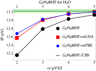
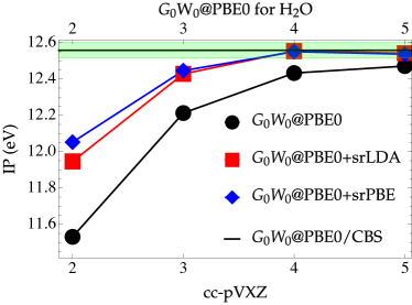
Figure 1: IP (in eV) of the water molecule computed at the $G_{0}W_{0}$ (black circles), $G_{0}W_{0}$+srLDA (red squares), and $G_{0}W_{0}$+srPBE (blue diamonds) levels of theory with increasingly large Dunning's basis sets Dunning (1989) (cc-pVDZ, cc-pVTZ, cc-pVQZ, and cc-pV5Z) with two different starting points: HF (left) and PBE0 (right). The thick black line represents the CBS value obtained by extrapolation (see text for more details). The green area corresponds to chemical accuracy (i.e, error below $1$ kcal/mol or $0.043$ eV).

IV Results and Discussion

In this section, we study a subset of atoms and molecules from the GW100 test set. van Setten et al. (2015) In particular, we study the 20 smallest molecules of the GW100 set, a subset that we label as GW20. This subset has been recently considered by Lewis and Berkelbach to study the effect of vertex corrections to $W$ on IPs of molecules. Lewis and Berkelbach (2019) Later in this section, we also study the five canonical nucleobases (adenine, cytosine, thymine, guanine, and uracil) which are also part of the GW100 test set.

IV.1 GW20

The IPs of the GW20 set obtained at the $G_{0}W_{0}$@HF and $G_{0}W_{0}$@PBE0 levels with increasingly larger Dunning's basis sets cc-pVXZ (X $=$ D, T, Q, and 5) are reported in Tables 1 and 2, respectively. The corresponding statistical deviations (with respect to the CBS values) are also reported: mean absolute deviation (MAD), root-mean-square deviation (RMSD), and maximum deviation (MAX). These reference CBS values have been obtained with the usual X^-3 extrapolation procedure using the three largest basis sets. Bruneval (2012)

The convergence of the IP of the water molecule with respect to the basis set size is depicted in Fig. 1. This represents a typical example. Additional graphs reporting the convergence of the IPs of each molecule of the GW20 subset at the $G_{0}W_{0}$@HF and $G_{0}W_{0}$@PBE0 levels are reported in the supporting information.

Tables 1 and 2 (as well as Fig. 1) clearly evidence that the present basis-set correction significantly increases the rate of convergence of IPs. At the $G_{0}W_{0}$@HF (see Table 1), the MAD of the conventional calculations (i.e, without basis-set correction) is roughly divided by two each time one increases the basis set size (MADs of $0.60$, $0.24$, $0.10$, and $0.05$ eV going from cc-pVDZ to cc-pV5Z) with maximum errors higher than $1$ eV for molecules such as HF, H2O, and LiF with the smallest basis set. Even with the largest quintuple-$\zeta$ basis, the MAD is still above chemical accuracy (i.e, error below $1$ kcal/mol or $0.043$ eV).

For each basis set, the correction brought by the short-range correlation functionals reduces by roughly half or more the MAD, RMSD, and MAX compared to the correction-free calculations. For example, we obtain MADs of $0.27$, $0.12$, $0.04$, and $0.01$ eV at the $G_{0}W_{0}$@HF+srPBE level with increasingly larger basis sets. Interestingly, in most cases, the srPBE correction is slightly larger than the srLDA one. This observation is clear at the cc-pVDZ level but, for larger basis sets, the two RS-DFT-based corrections are essentially equivalent. Note also that, in some cases, the corrected IPs slightly overshoot the CBS values. However, it is hard to know if it is not due to the extrapolation error. In a nutshell, the present basis-set correction provides cc-pVQZ quality results at the cc-pVTZ level. Besides, it allows to reach chemical accuracy with the quadruple-$\zeta$ basis set, an accuracy that could not be reached even with the cc-pV5Z basis set for the conventional calculations.

Very similar conclusions are drawn at the $G_{0}W_{0}$@PBE0 level (see Table 2) with a slightly faster convergence to the CBS limit. For example, at the $G_{0}W_{0}$@PBE0+srLDA/cc-pVQZ level, the MAD is only $0.02$ eV with a maximum error as small as $0.09$ eV.

It is worth pointing out that, for ground-state properties such as atomization and correlation energies, the density-based correction brought a larger acceleration of the basis-set convergence. For example, we evidenced in Ref. Loos et al., 2019 that quintuple-$\zeta$ quality atomization and correlation energies are recovered with triple-$\zeta$ basis sets. Here, the overall gain seems to be less important. The possible reasons for this could be: i) DFT approximations are usually less accurate for the potential than for the energy, Kim et al. (2013) and ii) because the present scheme only corrects the basis-set incompleteness error originating from the electron-electron cusp, some incompleteness remains at the HF or KS level. Adler et al. (2007)

Table 3: IPs (in eV) of the five canonical nucleobases (adenine, cytosine, thymine, guanine, and uracil) computed at the $G_{0}W_{0}$@PBE level of theory for various basis sets and corrections. The deviation with respect to the $G_{0}W_{0}$@PBE/def2-TQZVP extrapolated values are reported in square brackets. The extrapolation error is reported in parenthesis. Extrapolated $G_{0}W_{0}$@PBE results obtained with plane-wave basis sets, as well as CCSD(T) and experimental results are reported for comparison.

		IPs of nucleobases (eV)
Method	Basis	Adenine	Cytosine	Guanine	Thymine	Uracil
$G_{0}W_{0}$@PBE	def2-SVP	$7.27$[$-0.88$]	$7.53$[$-0.92$]	$6.95$[$-0.92$]	$8.02$[$-0.85$]	$8.38$[$-1.00$]
$G_{0}W_{0}$@PBE+srLDA	def2-SVP	$7.60$[$-0.55$]	$7.95$[$-0.50$]	$7.29$[$-0.59$]	$8.36$[$-0.51$]	$8.80$[$-0.58$]
$G_{0}W_{0}$@PBE+srPBE	def2-SVP	$7.64$[$-0.51$]	$8.06$[$-0.39$]	$7.34$[$-0.54$]	$8.41$[$-0.45$]	$8.91$[$-0.47$]
$G_{0}W_{0}$@PBE	def2-TZVP	$7.74$[$-0.41$]	$8.06$[$-0.39$]	$7.45$[$-0.42$]	$8.48$[$-0.38$]	$8.86$[$-0.52$]
$G_{0}W_{0}$@PBE+srLDA	def2-TZVP	$7.92$[$-0.23$]	$8.26$[$-0.19$]	$7.64$[$-0.23$]	$8.67$[$-0.20$]	$9.25$[$-0.13$]
$G_{0}W_{0}$@PBE+srPBE	def2-TZVP	$7.92$[$-0.23$]	$8.27$[$-0.18$]	$7.64$[$-0.23$]	$8.68$[$-0.19$]	$9.27$[$-0.11$]
$G_{0}W_{0}$@PBE	def2-QZVP	$7.98$[$-0.18$]	$8.29$[$-0.16$]	$7.69$[$-0.18$]	$8.71$[$-0.16$]	$9.22$[$-0.16$]
$G_{0}W_{0}$@PBE	def2-TQZVP	$8.16(1)$	$8.44(1)$	$7.87(1)$	$8.87(1)$	$9.38(1)$
$G_{0}W_{0}$@PBE	plane waves	$8.12$	$8.40$	$7.85$	$8.83$	$9.36$
$G_{0}W_{0}$@PBE	plane waves	$8.09(2)$	$8.40(2)$	$7.82(2)$	$8.82(2)$	$9.19(2)$
CCSD(T)	aug-cc-pVDZ	$8.40$	$8.76$	$8.09$	$9.04$	$9.43$
CCSD(T)	def2-TZVPP	$8.33$	$9.51$	$8.03$	$9.08$	$10.13$
Experiment		$8.48$	$8.94$	$8.24$	$9.20$	$9.68$

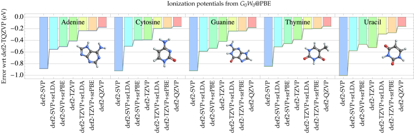
Figure 2: Error (in eV) with respect to the $G_{0}W_{0}$@PBE/def2-TQZVP extrapolated values for the IPs of the five canonical nucleobases (adenine, cytosine, thymine, guanine, and uracil) computed at the $G_{0}W_{0}$@PBE level of theory for various basis sets and corrections.

IV.2 Nucleobases

In order to check the transferability of the present observations to larger systems, we have computed the values of the IPs of the five canonical nucleobases (adenine, cytosine, thymine, guanine, and uracil) at the $G_{0}W_{0}$@PBE level of theory with a different basis set family. Weigend et al. (2003); Weigend and Ahlrichs (2005) The numerical values are reported in Table 3, and their error with respect to the $G_{0}W_{0}$@PBE/def2-TQZVP extrapolated values van Setten et al. (2015) (obtained via extrapolation of the def2-TZVP and def2-QZVP results) are shown in Fig. 2. Table 3 also contains extrapolated IPs obtained with plane-wave basis sets with two different software packages. Maggio et al. (2017); Govoni and Galli (2018) The CCSD(T)/def2-TZVPP computed by Krause et al. Krause et al. (2015) on the same geometries, the CCSD(T)//CCSD/aug-cc-pVDZ results from Ref. Roca-Sanjuan et al., 2006, as well as the experimental results extracted from Ref. van Setten et al., 2015 are reported for comparison purposes.

For these five systems, the IPs are all of the order of $8$ or $9$ eV with an amplitude of roughly $1$ eV between the smallest basis set (def2-SVP) and the CBS value. The conclusions that we have drawn in the previous subsection do apply here as well. For the smallest double-$\zeta$ basis def2-SVP, the basis-set correction reduces by roughly half an eV the basis-set incompleteness error. It is particularly interesting to note that the basis-set corrected def2-TZVP results are on par with the correction-free def2-QZVP numbers. This is quite remarkable as the number of basis functions jumps from $371$ to $777$ for the largest system (guanine).

V Conclusion

In the present manuscript, we have shown that the density-based basis-set correction developed by some of the authors in Ref. Giner et al., 2018 and applied recently to ground- and excited-state properties Loos et al. (2019); Giner et al. (2019) can also be successfully applied to Green function methods such as $GW$. In particular, we have evidenced that the present basis-set correction (which relies on LDA- or PBE-based short-range correlation functionals) significantly speeds up the convergence of IPs for small and larger molecules towards the CBS limit. These findings have been observed for different $GW$ starting points (HF, PBE, and PBE0). We have observed that the performance of the two short-range correlation functionals (srLDA and srPBE) are quite similar with a slight edge for srPBE over srLDA. Therefore, because srPBE is only slightly more computationally expensive than srLDA, we do recommend the use of srPBE.

As mentioned earlier, the present basis-set correction can be straightforwardly applied to other properties of interest such as electron affinities or fundamental gaps. It is also applicable to other flavors of $GW$ such as the partially self-consistent ev$GW$ or qs$GW$ methods, and more generally to any approximation of the self-energy. We are currently investigating the performance of the present approach within linear response theory in order to speed up the convergence of excitation energies obtained within the RPA and Bethe-Salpeter equation (BSE) Strinati (1988); Leng et al. (2016); Blase et al. (2018) formalisms. We hope to report on this in the near future.

Supporting Information

See supporting information for the expression of the short-range correlation potentials, additional graphs reporting the convergence of the ionization potentials of the GW20 subset with respect to the size of the basis set, and the numerical data of Tables 1 and 2 (provided in txt and json formats).