Double-Sparsity Learning Based Channel-and-Signal Estimation in Massive MIMO with Generalized Spatial Modulation

Abstract

In this paper, we study joint antenna activity detection, channel estimation, and multiuser detection for massive multiple-input multiple-output (MIMO) systems with general spatial modulation (GSM). We first establish a double-sparsity massive MIMO model by considering the channel sparsity of the massive MIMO channel and the signal sparsity of GSM. Based on the double-sparsity model, we formulate a blind detection problem. To solve the blind detection problem, we develop message-passing based blind channel-and-signal estimation (BCSE) algorithm. The BCSE algorithm basically follows the affine sparse matrix factorization technique, but with critical modifications to handle the double-sparsity property of the model. We show that the BCSE algorithm significantly outperforms the existing blind and training-based algorithms, and is able to closely approach the genie bounds (with either known channel or known signal). In the BCSE algorithm, short pilots are employed to remove the phase and permutation ambiguities after sparse matrix factorization. To utilize the short pilots more efficiently, we further develop the semi-blind channel-and-signal estimation (SBCSE) algorithm to incorporate the estimation of the phase and permutation ambiguities into the iterative message-passing process. We show that the SBCSE algorithm substantially outperforms the counterpart algorithms including the BCSE algorithm in the short-pilot regime.

I Introduction

Wireless transceivers with large antenna arrays and powerful signal processing capabilities have been proposed to accommodate the exponential growth of data traffics. The new wireless infrastructures generally require a significant increase of energy consumption in establishing communication links [2, 3]. As such, the energy efficiency (EE) of wireless transmission has attracted intensive research interests in recent years. Advanced technologies, such as massive multiple-input-multiple-output (MIMO) and spatial modulation (SM), have been developed to meet the EE requirement of next-generation wireless communication systems [4, 5, 6].

Massive MIMO with spatial modulation is a new communication paradigm consisting of a multi-antenna base station (BS) and multiple multi-antenna users, where the number of antennas at the BS is typically much greater than that at a user. In each time instance, every user activates only one antenna for signal transmission. Compared to conventional modulation techniques, spatial modulation is a promising solution for multi-antenna transmissions to reduce the power consumption, to relieve the burden of antenna synchronization, and to mitigate the inter-antenna interference. Recently, to achieve high spectrum efficiency, generalized spatial modulation (GSM) has been proposed to allow the activation of multiple antennas for simultaneous transmission of multiple independent symbols at each user [7].

A key challenge for GSM-based massive MIMO is how to carry out antenna activity detection, channel estimation, and mulituser detection at the BS. Most existing work assumes perfect channel state information (CSI) (or assumes that the CSI can be acquired from channel training in prior), and is focused on antenna activity detection and multiuser detection. For example, the author in [8] proposed a two-step approach: In the first step, the indices of active antennas are estimated using the ordered nearest minimum square-error detector; then in the second step, the signals are recovered based on the knowledge of the active antennas. In contrast to the two-step approach, the authors in [9] proposed a joint approach in which maximum likelihood (ML) detection is used to estimate both the indices of active antennas and the signals transmitted by these active antennas. However, the ML-based method suffers prohibitively high computational complexity as the size of a MIMO system scales up. Several low-complexity detectors with near-optimal performance was proposed in [10, 9].

More recently, researchers have proposed to design GSM-based massive MIMO systems by exploiting the signal sparsity inherent in spatial modulation [11, 12, 13, 14]. Specifically, the authors in [11] and [13] employed $l_{1}$ regularization based compressed sensing techniques [15] for the recovery of sparse signals. In [12], a message-passing algorithm was developed for joint antenna activity detection and multiuser detection. In [14], the authors proposed a generalized approximate message passing (GAMP) detector to deal with quantized measurements and spatial correlation in a large-scale antenna array at the BS.

The above mentioned approaches, however, have the following two limitations. First, all these approaches assume that the CSI is either a priori known to the receiver or estimated in a separate training stage prior to antenna activity detection and signal detection. In practice, the channel is unknown and the training-based method causes a significant pilot overhead when the MIMO size becomes large. Second, the structure of the massive MIMO channel, such as the angular-domain sparsity and the correlation in antenna arrays, has not been fully exploited in the existing algorithms.

In this paper, we study the transceiver design of the GSM-based massive MIMO system to address the above two limitations. We first establish a double-sparsity massive MIMO model by considering the correlation between transmit/receive antennas [16], the clustered channel sparsity in the angular domain [17], and the signal sparsity inherent in GSM. Specifically, the received signal can be represented as $\mathbf{Y}=\mathbf{A}_{\textsf{R}}{\mathbf{G}}{\mathbf{A}}_{\textsf{T}}^{H}\mathbf{X}+\mathbf{N}$, where $\mathbf{A}_{\textsf{R}}$ and ${\mathbf{A}}_{\textsf{T}}$ are steering vector matrices characterizing the receive and transmit correlations, respectively, ${\mathbf{G}}$ is a sparse angular-domain channel matrix, $\mathbf{X}$ is a sparse signal matrix with GSM, and $\mathbf{N}$ is an ambient noise matrix. With the knowledge of $\mathbf{A}_{\textsf{R}}$ and $\mathbf{A}_{\textsf{T}}$, the joint estimation of the sparse matrices $\mathbf{G}$ and $\mathbf{X}$ from $\mathbf{Y}$ is a bilinear recovery problem. It seems that the parametric bilinear generalized approximate message passing (P-BiGAMP) algorithm [18] can be applied to this problem by vectorizing $\mathbf{Y}$, $\mathbf{G}$, and $\mathbf{X}$. However, we find that the P-BiGAMP algorithm does not work in our problem, probably because the matrix product $\mathbf{A}_{\textsf{R}}\mathbf{G}\mathbf{A}_{\textsf{T}}^{H}\mathbf{X}$ here does not satisfy the requirement of random measurements by P-BiGAMP. To address this issue, we formulate a blind detection problem by absorbing ${\mathbf{A}}_{\textsf{T}}^{H}$ into the matrix either on the right or on the left in sparse matrix factorization. To solve the blind detection problem, we develop a message passing based blind channel-and-signal estimation (BCSE) algorithm that performs antenna activity activation, channel estimation, and user detection simultaneously. We show that although the basic idea is borrowed from the affine sparse matrix factorization (ASMF) algorithm developed in [19], new initialization and and re-initialization methods are necessary to ensure a good algorithm performance for the considered double-sparsity model. We also show that our proposed scheme significantly outperforms the other blind detection schemes [20, 21] (that exploit either the channel sparsity or the signal sparsity, but not both) and the state-of-the-art training-based schemes for massive MIMO systems with GSM [22].

Similar to the schemes developed in [19, 20, 21], sparse matrix factorization suffers from the so-called phase and permutation ambiguities. In the BCSE algorithm, reference symbols and antenna labels are used to eliminate the phase and permutation ambiguities after matrix factorization. Similar to the pilot signals in a training-based scheme, the reference symbols and the antenna labels are a priori known by the receiver. Therefore, they can be incorporated into the iterative detection process for performance enhancement, rather than used for compensation afterwards. As such, we develop a semi-blind channel-and-signal estimation (SBCSE) algorithm by treating the reference symbols and the antenna labels as short pilots. Based on the framework of BCSE, we introduce two extra steps in the SBCSE algorithm: We use the short pilots to eliminate the phase and permutation ambiguities in the output of BCSE, and then use compressed sensing techniques to further refine the channel estimate based on the structured sparsity of the massive MIMO channel. Numerical results demonstrate that the proposed SBCSE algorithm substantially outperforms the state-of-the-art counterpart algorithms including the BCSE algorithm in the short-pilot regime.

To summarise, the main contributions of this paper are listed as follows:

• To the best of our knowledge, this is the first work to consider joint antenna activity detection, channel estimation, and multiuser detection based on the double-sparsity model for GSM-based massive MIMO systems. We establish a comprehensive probability model to characterize the channel sparsity inherent in the massive MIMO channel and the signal sparsity inherent in GSM, based on which the joint estimation problem is defined.

• We develop a message-passing based blind detection algorithm, termed the BCSE algorithm, to efficiently exploit the channel sparsity and the signal sparsity. We show that the BCSE algorithm significantly outperforms the existing blind and training-based algorithms, and is able to closely approach the genie bounds (with either known channel or known signal).

• To utilize the pilot signals (including the reference symbols and the user labels) more efficiently, we further develop a semi-blind detection algorithm, termed SBCSE. We show that the SBCSE algorithm substantially outperforms the counterpart algorithms including the BCSE algorithm in the short-pilot regime.

The rest of this paper is organized as follows. Section II describes the GSM-based massive MIMO systems. Section III and Section IV present the proposed blind and semi-blind channel-and-signal estimation algorithms, respectively. We discuss the parameter learning and the complexity of the proposed algorithms in Section V. Numerical results are presented in Section VI. Conclusions are drawn in Section VII.

Notation: Regular letters, lowercase bold letters, and capital bold letters represent scalars, vectors, and matrices, respectively. The superscripts $(\cdot)^{H}$, $(\cdot)^{*}$, $(\cdot)^{T}$, and $(\cdot)^{-1}$ represent the conjugate transpose, the conjugate, the transpose, and the inverse of a matrix, respectively; $|\cdot|$ represents the cardinality of a set; $\|\cdot\|_{0}$ denotes the $l_{0}$ norm; $\|\cdot\|_{1}$ denotes the $l_{1}$ norm; $\|\cdot\|_{F}$ denotes the Frobenius norm. $\rm diag\{\mathbf{a}\}$ represents the diagonal matrix with the diagonal entries specified by $\mathbf{a}$. $\otimes$ denotes the Kronecker product and $\delta(\cdot)$ denotes the Dirac delta function. $\mathbf{I}_{N}$ denotes the identity matrix of size $N\times N$. Some frequently used symbols are listed in the Table I.

TABLE I: Frequently used symbols

$n$	transmit-antenna index	$m$	receive-antenna index
$k$	user index	$t$	time slot index
$K$	number of users	$T$	coherence time
$M$	number of antennas at receiver	$M^{{}^{\prime}}$	number of AoA bins
$N$	number of antennas at each user	$N^{{}^{\prime}}$	number of AoD bins
$\bm{\theta}$	collection of AoAs	$\bm{\phi}$	collection of AoDs
$\bm{\vartheta}$	angular grid of AoAs	$\bm{\varphi}$	angular grid of AoDs
$\mathbf{a}_{\text{R}}$	steering vector at receiver	$\mathbf{a}_{\text{T}}$	steering vector at transmitter
$\mathbf{A}_{\textsf{R}}$	steering-vector matrix at receiver	$\mathbf{A}_{\textsf{T}}$	steering-vector matrix at transmitter
$\lambda$	sparsity level of the channel $\mathbf{G}$	$\rho$	sparsity level of the signal
$q$	index of AoA bins	$p$	index of AoD bins

II System Model

II-A GSM-Based Massive MIMO Systems

We consider a multiple access system, in which $K$ users communicate with a single BS equipped with $M$ receive antennas. $M$ is usually in the order of tens to hundreds. Each user is equipped with $N$ transmit antennas and employs GSM [7, 14]. That is, at any time slot and for any user, each transmit antenna either transmits a symbol taken from a modulation alphabet $\cal A$ or remains inactive (or in other words, transmits a zero symbol). Specifically, let $c_{k,n,t}$ be the indicator of the activity state of antenna $n$ of user $k$ at time slot $t$, i.e.,

$$c_{k,n,t}=\Bigg{\{}\begin{array}[]{cl}1,&\text{antenna $n$ of}\ \text{user}\ k\ \text{is active}\\ 0,&\text{otherwise}\end{array}$$ (3)

and $x_{k,n,t}$ be the symbol transmitted by antenna $n$ of user $k$ at time slot $t$. Note that $x_{k,n,t}\in\cal A$ if $c_{k,n,t}=1$, and $x_{k,n,t}=0$ if $c_{k,n,t}=0$. We assume that $\{c_{k,n,t}\}$ are independently and identically distributed, and so are $\{x_{k,n,t}\}$. In particular, each $x_{k,n,t}$ is independently drawn from the distribution of

$$p(x)=\frac{\rho}{|\cal A|}\sum_{a\in\cal A}\delta(x-a)+(1-\rho)\delta(x),$$ (4)

where $\rho\in(0,1)$ is the signal sparsity level and $|\cal A|$ is the size of $\cal A$. Note that both $\rho$ and $\cal A$ are known to the receiver. We assume that the average power of $\cal A$ is normalized, i.e., $\frac{\sum_{a\in{\cal A}}|a|^{2}}{|\cal A|}=1$. Clearly, each antenna transmits $H_{\rho}$ bits per time slot, where

$$H_{\rho}=-(1-\rho)\log_{2}(1-\rho)-\rho\log_{2}\left(\frac{\rho}{|\cal A|}\right).$$ (5)

Denote by $\mathbf{x}_{k,t}=[x_{k,1,t},\cdots,x_{k,N,t}]^{T}$ the $k$-th user’s symbol vector at time slot $t$. We stack all the symbol vectors from the $K$ users at time slot $t$ as

$${\mathbf{x}}_{t}=[{\mathbf{x}}_{1,t}^{T},{\mathbf{x}}_{2,t}^{T},\cdots,\mathbf{x}_{K,t}^{T}]^{T}\in\mathbb{C}^{KN\times 1}.$$ (6)

Correspondingly, denote $\mathbf{H}\triangleq[\mathbf{h}_{1},\cdots,\mathbf{h}_{KN}]\in\mathbb{C}^{M\times KN}$, where $\mathbf{h}_{(k-1)N+n}=[h_{1,(k-1)N+n},$ $h_{2,(k-1)N+n},\cdots,h_{M,(k-1)N+n}]^{T}\in\mathbb{C}^{M\times 1}$ is the flat fading channel coefficient vector from antenna $n$ of user $k$ to the BS. At time slot $t$, the received signal at the BS is given by

$${\mathbf{y}}_{t}=\mathbf{H}{\mathbf{x}}_{t}+\mathbf{n}_{t},$$ (7)

where $\mathbf{n}_{t}$ is the AWGN noise following the complex circularly symmetric Gaussian distribution with mean zero and covariance $\sigma^{2}\mathbf{I}$ with $\sigma^{2}$ being the noise power and $\mathbf{I}$ being the identity matrix of an appropriate size. We assume block fading with coherence time $T$, i.e., the channel remains unchanged for time duration of $T$. Collecting all the received signals of $T$ successive time slots, we express the received signal at the BS as

$$\mathbf{Y}=\mathbf{H}\mathbf{X}+\mathbf{N},$$ (8)

where $\mathbf{Y}=[\mathbf{y}_{1},\mathbf{y}_{2},\cdots,\mathbf{y}_{T}]$, $\mathbf{X}=[{\mathbf{x}}_{1},\cdots,{\mathbf{x}}_{T}]$, and $\mathbf{N}=[\mathbf{n}_{1},\mathbf{n}_{2},\cdots,\mathbf{n}_{T}]$. The system model in (8) is illustrated in Fig. 1.

II-B Angular-Domain Channel Model

We start with describing the channel representation in the angular domain. During coherence time $T$, the uplink channel from user $k$ to the BS can be modelled as

$$\mathbf{H}_{k}=\sum_{i=1}^{L_{k,c}}\sum_{j=1}^{L_{k,p}}\alpha_{k}(i,j)\mathbf{a}_{{\textsf{R}}}(\theta_{k}(i,j))\mathbf{a}_{\textsf{T}}^{H}(\phi_{k}(i,j)),$$ (9)

where $L_{k,c}$ and $L_{k,p}$ denote the number of scattering clusters and the number of physical paths in each cluster between user $k$ and the BS, respectively; $\alpha_{k}(i,j)$ is the channel complex gain of path $j$ in cluster $i$ for user $k$; $\mathbf{a}_{{\textsf{R}}}(\theta_{k}(i,j))$ and $\mathbf{a}_{{\textsf{T}}}(\phi_{k}(i,j))$ are the steering vectors with $\theta_{k}$ being the angle of arrival (AoA) of BS and $\phi_{k}$ being the angle of departure (AoD) of user $k$, respectively. For notational convenience, denote by $\bm{\theta}_{k}=\{\theta_{k}(i,j)\}_{\forall i,j}$ the collection of true AoAs and $\bm{\phi}_{k}=\{\phi_{k}(i,j)\}_{\forall i,j}$ the collection of true AoDs of user $k$. In general, $\mathbf{a}_{{\textsf{R}}}(\theta_{k})$ and $\mathbf{a}_{\textsf{T}}(\phi_{k})$ are determined by the geometry of the antenna arrays at the BS and the users, respectively. For convenience of discussion, we focus on the case that both the BS and the users are equipped with uniform linear arrays (ULAs). Let $d_{\textsf{R}}$ and $d_{\textsf{T}}$ denote the antenna spacing at the BS and at each user, respectively. Then, the corresponding steering vectors are given by

$$\mathbf{a}_{\textsf{R}}(\theta_{k}) =\frac{1}{\sqrt{M}}\left[1,e^{-j2\pi\frac{d_{\textsf{R}}\sin\theta_{k}}{\varrho}},\cdots,e^{-j2\pi\frac{(M-1)d_{\textsf{R}}\sin\theta_{k}}{\varrho}}\right]^{T}$$

$$\mathbf{a}_{\textsf{T}}(\phi_{k}) =\frac{1}{\sqrt{N}}\left[1,e^{-j2\pi\frac{d_{\textsf{T}}\sin\phi_{k}}{\varrho}},\cdots,e^{-j2\pi\frac{(N-1)d_{\textsf{T}}\sin\phi_{k}}{\varrho}}\right]^{T},$$ (10)

where $\varrho$ is the wavelength of propagation, $\theta_{k}\in\left(-\frac{\pi}{2},\frac{\pi}{2}\right)$, and $\phi_{k}\in\left(-\frac{\pi}{2},\frac{\pi}{2}\right)$. Note that the work in this paper can be readily extended to antenna arrays with other geometries, such as lens antenna arrays (LAA) [19] and 2-dimensional antenna arrays [23].

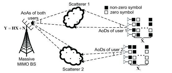
Figure 1: The illustration of a massive MIMO system with GSM for $K=2$ users.

The model parameters $\{{\bm{\theta}}_{k},{\bm{\phi}}_{k},{L_{k,c}},{L_{k,p}}\}$ are difficult to acquire in practice. To avoid this difficulty, we introduce the so-called virtual channel representation of (9). Let ${\bm{\vartheta}}=\{{\vartheta}_{q}\}{}_{q=1}^{M^{{}^{\prime}}}$ be a given grid that consists of $M^{{}^{\prime}}$ discrete angular bins ranging from $-\frac{\pi}{2}$ to $\frac{\pi}{2}$. Similarly, let ${\bm{\varphi}_{k}}=\{\varphi_{k,p}\}_{p=1}^{N^{{}^{\prime}}}$ be a given grid that consists of $N^{{}^{\prime}}$ discrete angular bins ranging from $-\frac{\pi}{2}$ to $\frac{\pi}{2}$. For sufficiently large $M^{{}^{\prime}}$ and $N^{{}^{\prime}}$, $\mathbf{H}_{k}$ can be well approximated in the virtual AoA and AoD domain by

$$\mathbf{H}_{k} =\sum_{q=1}^{M^{{}^{\prime}}}\sum_{p=1}^{N^{{}^{\prime}}}g_{k}(q,p){\mathbf{a}}_{\textsf{R}}({\vartheta}_{q}){\mathbf{a}}_{\textsf{T}}^{H}({\varphi}_{k,p})$$

$$=\mathbf{A}_{\textsf{R}}({\bm{\vartheta}})\mathbf{G}_{k}\mathbf{A}_{\textsf{T,k}}^{H}({\bm{\varphi}_{k}}),$$ (11)

where $\mathbf{G}_{k}\in\mathbb{C}^{M^{{}^{\prime}}\times N^{{}^{\prime}}}$ is the virtual angular-domain channel matrix with the $(q,p)$-th element given by $g_{k}(q,p)$, $\mathbf{A}_{\textsf{R}}({\bm{\vartheta}})\triangleq[\mathbf{a}_{\textsf{R}}({\vartheta}_{1}),\cdots,\mathbf{a}_{\textsf{R}}({\vartheta}_{M^{{}^{\prime}}})]\in\mathbb{C}^{M\times M^{{}^{\prime}}}$, and $\mathbf{A}_{\textsf{T,k}}({\bm{\varphi}}_{k})\triangleq[\mathbf{a}_{\textsf{T}}({\varphi}_{k,1}),\cdots,\mathbf{a}_{\textsf{T}}({\varphi}_{k,N^{{}^{\prime}}})]$ $\in\mathbb{C}^{N\times N^{{}^{\prime}}}$. With (II-B), the received signal at the BS in (8) can be represented as

$$\mathbf{Y} =\mathbf{H}\mathbf{X}+\mathbf{N}$$ (12a)

$$=\mathbf{A}_{\textsf{R}}({\bm{\vartheta}}){\mathbf{G}}{\mathbf{A}}_{\textsf{T}}^{H}({\bm{\varphi}})\mathbf{X}+\mathbf{N},$$ (12b)

where ${\mathbf{G}}=[{\mathbf{G}}_{1},\cdots,{\mathbf{G}}_{K}]\in\mathbb{C}^{M^{{}^{\prime}}\times KN^{{}^{\prime}}}$, and ${\mathbf{A}}_{\textsf{T}}({\bm{\varphi}})={\rm diag}\{\mathbf{A}_{\textsf{T,1}}({\bm{\varphi}}_{1}),\cdots,\mathbf{A}_{\textsf{T,K}}({\bm{\varphi}}_{K})\}\in\mathbb{C}^{KN\times KN^{{}^{\prime}}}$. Note that the electromagnetic signal of a user usually impinges upon or departs from an antenna array in a limited number of angular bins, implying that a large portion of the elements of $\mathbf{G}$ are zero, i.e., $\mathbf{G}$ is a sparse matrix. Define the sparsity level of $\mathbf{G}$ as

$$\lambda =\frac{\|\mathbf{G}\|_{0}}{M^{{}^{\prime}}N^{{}^{\prime}}K},$$ (13)

where $\|\cdot\|_{0}$ denotes the $l_{0}$ norm. The system model in (12b) involves two sparse matrices $\mathbf{X}$ and $\mathbf{G}$, hence the name double-sparsity model.

II-C Probability Model of $\mathbf{G}$

Let $\mathbf{D}_{k}\in\mathbb{C}^{M^{{}^{\prime}}\times N^{{}^{\prime}}}$ be the channel support matrix of user $k$ and $d_{k,q,p}$ be the $(q,p)$-th entry of $\mathbf{D}_{k}$, where $d_{k,q,p}=0$ (or 1) indicates that the corresponding entry $g_{k,q,p}$ of $\mathbf{G}_{k}$ is zero (or non-zero). Following [24], we assume that the entries of $\mathbf{G}_{k}$ conditioned on $\mathbf{D}_{k}$ are independent of each other, with the distribution given by

$$p(\mathbf{G}_{k}|\mathbf{D}_{k}) =\prod_{q=1}^{M^{{}^{\prime}}}\prod_{p=1}^{N^{{}^{\prime}}}\left((1-d_{k,q,p})\delta(g_{k,q,p})+d_{k,q,p}{\cal C}{\cal N}\left(g_{k,q,p};0,v_{\rm pri}\right)\right),$$ (14)

where $v_{\rm pri}$ is the variance of the non-zero entries of $\mathbf{G}_{k}$. Note that $v_{\rm pri}$ is determined by the large-scale fading of user $k$, and is generally unknown to the receiver.

Due to the limited number of scatterers in the propagation environment, the massive MIMO channels exhibit the property of clustered sparsity, i.e., the non-zero entries of $\mathbf{G}$ usually gather in clusters, with each cluster corresponding to a scatterer, as illustrated in Fig. 1. To exploit the clustered sparsity, we shall introduce Markov model to capture the scattering structure at the transmitter and the receiver [24].

III Blind Channel-and-Signal Estimation

III-A Problem Formulation

Blind channel-and-signal estimation aims to estimate $\mathbf{H}$ and $\mathbf{X}$ from the observed data matrix $\mathbf{Y}$ in (12), without using any pilot signals. This problem can be formulated as

$$(\hat{\mathbf{H}},\hat{\mathbf{X}}) =\arg\max_{\mathbf{H},\mathbf{X}}p(\mathbf{X},\mathbf{H}|\mathbf{Y}).$$ (15)

To solve (15), our previous work proposed to factorize the noisy product $\mathbf{Y}$ by exploiting either the channel sparsity [20, 19] or the signal sparsity [21]. Sparse matrix factorization techniques, such as the K-SVD algorithm [25], the SPAMS algorithm [26], the ER-SpUD algorithm [27], and the bilinear generalized approximate message passing (BiG-AMP) algorithm [28], can be used to produce the estimates of $\mathbf{H}$ and $\mathbf{X}$ simultaneously. It has been shown in [20, 19], and [21] that the blind estimation approach suffers from phase and permutation ambiguities. More specifically, denote by $\bm{\Sigma}$ a unitary diagonal matrix with the phases of the diagonal entries randomly selected from $\Omega$ (see footnote 2 for the definition of $\Omega$). Denote by $\bm{\Pi}$ an arbitrary permutation matrix. The phase and permutation ambiguities are due to the fact that if $(\hat{\mathbf{H}},\hat{\mathbf{X}})$ is a solution to (15), then $(\tilde{\mathbf{H}}=\hat{\mathbf{H}}\bm{\Pi}^{-1}\bm{\Sigma}^{-1},\bm{\Sigma}\bm{\Pi}\hat{\mathbf{X}})$ is also a valid solution to (15). The ambiguity issue has the following two consequences for blind detection. On the one hand, the solution of (15) is not unique, and thus extra resources (such as reference signals and user labels) are required to eliminate the ambiguities after performing matrix factorization. On the other hand, the existence of the ambiguities facilitates the design of efficient iterative algorithms to find equally good solutions. In fact, it has been shown in [29] that gradient-based iterative algorithms can find a globally optimal solution of the non-convex sparse matrix factorization problem, provided that certain regularity conditions are satisfied.

The approaches in [20, 19], and [21], however, fail to exploit the double-sparsity property of the model in (12). With this regard, we aim to design an efficient blind channel-and-signal estimation algorithm that can simultaneously exploit the sparsity of both channel matrix $\mathbf{G}$ and signal matrix $\mathbf{X}$. Rewrite $\mathbf{Y}$ in (12) in its vectorized form as

$${\rm vec}(\mathbf{Y}) =\sum_{q,p}\sum_{l}g_{q,p}\mathbf{z}_{q,p,l}x_{l}+{\rm vec}(\mathbf{N}),$$ (16)

where $g_{q,p}$ is the $(q,p)$-th element of $\mathbf{G}$, $x_{l}$ is the $l$-th element of ${\rm vec}(\mathbf{X})$, $\mathbf{z}_{q,p,l}\in\mathbb{C}^{MT}$ is the $l$-th column of $(\mathbf{I}_{T}\otimes\mathbf{B}_{q,p})$, where $\mathbf{B}_{q,p}\triangleq\mathbf{a}_{\textsf{R},q}({{\vartheta}_{q}}){\mathbf{a}}_{\textsf{T},p}^{H}({{\varphi}_{p}})\in\mathbb{C}^{M\times KN}$, and $\mathbf{a}_{\textsf{R},q}({{\vartheta}_{q}})$ and ${\mathbf{a}}_{\textsf{T},p}^{H}({{\varphi}_{p}})$ are respectively the $q$-th column of $\mathbf{A}_{\textsf{R}}({\bm{\vartheta}})$ and the $p$-th row of ${\mathbf{A}}_{\textsf{T}}^{H}({\bm{\varphi}})$. With the measurements in (16), it seems that the joint estimation of $\mathbf{G}$ and $\mathbf{X}$ can be solved by the parametric bilinear generalized approximate message passing (P-BiGAMP) algorithm [18]. However, through extensive simulations, we observe that the P-BiGAMP algorithm do not work in factorizing the sparse matrices $\mathbf{G}$ and $\mathbf{X}$. For the P-BiGAMP algorithm, we conjecture the main reason as follows. Due to the existence of the known matrix $\mathbf{A}_{\textsf{T}}(\mathbf{\bm{\varphi}})$ between $\mathbf{G}$ and $\mathbf{X}$ in (12b), the aforementioned phase and permutation ambiguities [20] no longer exist. In other words, the solution to the factorization of $\mathbf{G}$ and $\mathbf{X}$ based on $\mathbf{Y}$ in (12) is unique up to a scalar phase shift. With such uniqueness of the solution, the P-BiGAMP algorithm is prone to be struck at a local optimum. One way to avoid the above difficulty is to absorb $\mathbf{A}_{\textsf{T}}(\bm{\varphi})$ into the matrix either on the right or on the left in sparse matrix factorization. Along this line, we consider the following three approaches for blind channel-and-signal estimation.

1. We first consider a simplified DFT-based signal model. We project the received signal matrix to the angular domain by the inverse DFT unitary transform, i.e.

   $$\mathbf{Y}^{{}^{\prime}} =\mathbf{F}^{H}\mathbf{Y}$$

   $$=\mathbf{F}^{H}\mathbf{A}_{\textsf{R}}({\bm{\vartheta}}){\mathbf{G}}{\mathbf{A}}_{\textsf{T}}^{H}({\bm{\varphi}})\mathbf{X}+\mathbf{F}^{H}\mathbf{N}$$

   $$=\mathbf{F}^{H}\mathbf{A}_{\textsf{R}}({\bm{\vartheta}})\mathbf{S}\mathbf{X}+\mathbf{N}^{{}^{\prime}},$$ (17)

   where $\mathbf{S}=\mathbf{G}\mathbf{A}_{\textsf{T}}^{H}(\bm{\varphi})$, and $\mathbf{N}^{{}^{\prime}}=\mathbf{F}^{H}\mathbf{N}$. Suppose that the channel AoAs are located on a uniform sampling grid for virtual spatial angles, i.e.

   $$\sin\vartheta_{q}=\frac{q-1}{M^{{}^{\prime}}},\textrm{for}\;q=1,\cdots,M^{{}^{\prime}}=M.$$ (18)

   Substituting (18) into (1), we see that $\mathbf{A}_{\textsf{R}}(\bm{\vartheta})$ is the normalized DFT matrix. Then $\mathbf{F}^{H}\mathbf{A}_{\textsf{R}}({\bm{\vartheta}})$ becomes the identity matrix. Thus, we can estimate both $\mathbf{S}$ and $\mathbf{X}$ by directly factorizing $\mathbf{Y}^{{}^{\prime}}$, which can be accomplished by using the BiGAMP algorithm. However, the AoAs are generally not on the grid in practice. This DFT-based method (in which the estimates of $\mathbf{S}$ and $\mathbf{X}$ are obtained by treating $\mathbf{Y}^{{}^{\prime}}$ modelled as $\mathbf{Y}^{{}^{\prime}}=\mathbf{S}\mathbf{X}+\mathbf{N}^{{}^{\prime}}$) always suffers performance loss due to the unavoidable AoA mismatch, i.e. $\mathbf{F}^{H}\mathbf{A}_{\textsf{R}}({\bm{\vartheta}})$ is actually not the identity matrix.

2. Alternatively, we absorb $\mathbf{A}_{\textsf{T}}(\bm{\varphi})$ into the right by letting $\tilde{\mathbf{X}}\triangleq\mathbf{A}_{\textsf{T}}^{H}({\bm{\varphi}})\mathbf{X}\in\mathbb{C}^{KN^{{}^{\prime}}\times T}$. Then,

   $$\mathbf{Y} =\mathbf{A}_{\textsf{R}}({\bm{\vartheta}}){\mathbf{G}}\tilde{\mathbf{X}}+\mathbf{N}.$$ (19)

   We follow the affine sparse matrix factorization approach in [19] to produce the estimates of $\mathbf{G}$ and $\tilde{\mathbf{X}}$ based on $\mathbf{Y}$ in (19) and the sparsity of $\mathbf{G}$ and $\tilde{\mathbf{X}}$. However, due to the mixing effect of $\mathbf{A}_{\textsf{T}}(\bm{\varphi})$, the entries of $\tilde{\mathbf{X}}$ are generally not constrained on the alphabet $\cal A$. Such a loss of constellation constraints leads to performance degradation in matrix factorization.

3. To avoid the loss of constellation information, we absorb $\mathbf{A}_{\textsf{T}}(\bm{\varphi})$ into the left matrix. The system model is given by

   $$\mathbf{Y} =\mathbf{A}_{\textsf{R}}({\bm{\vartheta}}){\mathbf{S}}\mathbf{X}+\mathbf{N}.$$ (20)

   We still follow the affine sparse matrix factorization approach in [19] to estimate $\mathbf{S}$ and $\mathbf{X}$ based on $\mathbf{Y}$. The only differences are that here both $\mathbf{S}$ and $\mathbf{X}$ are sparse and that the entries of $\mathbf{X}$ are constrained on $\cal{A}$. These properties can be exploited to improve the performance of matrix factorization.

It is clear that all the models in (1)-(20) involve the factorization of two sparse matrices. In the following, we focus on the model in (20) to present the blind channel-and-signal estimation (BCSE) algorithm. The BCSE algorithm can be applied to the models (1) and (19) with some minor modifications. We will provide numerical evidences to show that the algorithm developed based on (20) significantly outperform those based on (1) and (19).

The affine sparse matrix factorization (ASMF) problem described above can be formulated as

$$(\hat{\mathbf{S}},\hat{\mathbf{X}})=\arg\max_{{\mathbf{S}},\mathbf{X}}p({\mathbf{S}},\mathbf{X}|\mathbf{Y};\bm{\psi}),$$ (21)

where $\bm{\psi}\triangleq\{{\bm{\vartheta}},\rho,\lambda_{{S}},p_{01}^{{S}},p_{10}^{{S}},v_{{S}},\sigma^{2}\}$, $\lambda_{{S}}$ is the sparsity level of $\mathbf{S}$, $p_{01}^{{S}}$ and $p_{10}^{{S}}$ are the transition probabilities of the Markov chain characterizing the support structure of $\mathbf{S}$, and $v_{{S}}$ is the variance of the non-zero entries of $\mathbf{S}$. Here, the parameters in $\bm{\psi}$ are assumed to be known when solving (21). The estimation of these parameters will be discussed later in Section V. The problem in (21) is generally difficult to solve. In the following, we present a low-complexity approximate solution based on the message passing principle.

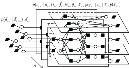
Figure 2: An example of the factor graph for $M=3$, $T=4$, where hallow circles and black rectangles represent variable nodes and factor nodes, respectively, $f_{q,t}=\delta(w_{q,t}-\sum_{p=1}^{KN}s_{q,p}x_{p,t})$, $g_{m,t}=\delta(z_{m,t}-\sum_{q=1}^{M^{{}^{\prime}}}A_{m,q}{w}_{q,t})$.

III-B Factor Graph Representation

To start with, we describe the factor graph representation of the probability distribution involved in (21) as follows. Recall that the entries of $\mathbf{X}_{k}$ are independently and uniformly drawn from the distribution in (4). Thus,

$$p(\mathbf{X}_{k}) =\prod_{n=1}^{N}\prod_{t=1}^{T}p(x_{k,n,t}).$$ (22)

Define $\mathbf{Z}\triangleq\mathbf{A}_{\textsf{R}}(\bm{\vartheta})\mathbf{S}\mathbf{X}\in\mathbb{C}^{M\times T}$. Since $\mathbf{N}$ is an AWGN, we have

$$p(\mathbf{Y}|\mathbf{\mathbf{Z}}) =\prod_{m=1}^{M}\prod_{t=1}^{T}{\cal C\cal N}(y_{m,t};z_{m,t},\sigma^{2}).$$ (23)

Due to the mixing effect of $\mathbf{A}_{\textsf{T}}(\bm{\varphi})$, the Markovity of the support of $\mathbf{S}=\mathbf{G}\mathbf{A}_{\textsf{T}}^{H}(\bm{\varphi})$ cannot be directly described by the AoD and AoA random vectors introduced in Section II-C. Instead, let $\mathbf{D}^{{}^{\prime}}$ denote the support of $\mathbf{S}$. We use an independent Markov chain to describe the probability distribution of each column of $\mathbf{D}^{{}^{\prime}}$, yielding

$$p(\mathbf{D}^{{}^{\prime}}) =\prod_{p=1}^{KN}\left(p(d_{1,p}^{{}^{\prime}})\prod_{q=2}^{M^{{}^{\prime}}}p(d_{q,p}^{{}^{\prime}}|d_{q-1,p}^{{}^{\prime}})\right),$$ (24)

where the transition probabilities are given by $p(d_{q,p}^{{}^{\prime}}|d_{q-1,p}^{{}^{\prime}}=0)=p_{10}^{{S}}\delta(d_{q,p}^{{}^{\prime}}-1)+(1-p_{10}^{{S}})\delta(d_{q,p}^{{}^{\prime}})$ and $p(d_{q,p}^{{}^{\prime}}|d_{q-1,p}^{{}^{\prime}}=1)=p_{01}^{{S}}\delta(d_{q,p}^{{}^{\prime}})+(1-p_{01}^{{S}})\delta(d_{q,p}^{{}^{\prime}}-1)$. The initial $p(d_{1,p}^{{}^{\prime}})$ is set as $p(d_{1,p}^{{}^{\prime}})=\lambda_{S}\delta(d_{1,p}^{{}^{\prime}}-1)+(1-\lambda_{S})\delta(d_{1,p}^{{}^{\prime}})$. Then, the joint probability density distribution of $({\mathbf{S}},\mathbf{X})$ conditioning on $\mathbf{Y}$ is given by

$$p({\mathbf{S}},\mathbf{X},\mathbf{Z},\mathbf{W}|\mathbf{Y})\propto p(\mathbf{Y}|\mathbf{Z})p(\mathbf{X})p({\mathbf{S}}|\mathbf{D}^{{}^{\prime}})p(\mathbf{D}^{{}^{\prime}})\delta(\mathbf{Z}-\mathbf{A}_{\textsf{R}}(\bm{\vartheta})\mathbf{W})\delta(\mathbf{W}-{\mathbf{S}}\mathbf{X})$$

$$=\left(\prod_{m=1}^{M}\prod_{t=1}^{T}p(y_{m,t}|z_{m,t})\delta(z_{m,t}-\sum_{q=1}^{M^{{}^{\prime}}}A_{m,q}{w}_{q,t})\delta(w_{q,t}-\sum_{p=1}^{KN}s_{q,p}{x}_{p,t})\right)\left(\prod_{p=1}^{KN}\prod_{t=1}^{T}p_{x_{p,t}}(x_{p,t})\right)$$

$$\quad\times\left(\prod_{q=1}^{M^{{}^{\prime}}}\prod_{p=1}^{KN}p(s_{q,p}|d_{q,p}^{{}^{\prime}})\right)\!\!\left(\prod_{p=1}^{KN}\left(p(d_{1,p}^{{}^{\prime}})\prod_{q=2}^{M^{{}^{\prime}}}p(d_{q,p}^{{}^{\prime}}|d_{q-1,p}^{{}^{\prime}})\right)\!\right),$$ (25)

where $A_{m,q}$ is the $(m,q)$-th element of $\mathbf{A}_{\textsf{R}}(\bm{\vartheta})$. The factor graph representation of (III-B) is depicted in Fig. 2, where the variable nodes consist of $\{z_{m,t}\}$, $\{w_{q,t}\}$, $\{{s}_{q,p}\}$, $\{{d}_{q,p}^{{}^{\prime}}\}$, $\{x_{p,t}\}$, and the check nodes consist of $\{f_{q,t}\}$, $\{g_{m,t}\}$, $\{p(x_{p,t})\}$, $\{p({s}_{q,p})\}$, $\{p(y_{m,t}|z_{m,t})\}$, and $\{p(d_{q,p}^{{}^{\prime}}|d_{q-1,p}^{{}^{\prime}})\}$.

III-C Blind Channel-and-Signal Estimation Algorithm

Algorithm 1 : BCSE algorithm

1:Input: received signal $\mathbf{Y}$, parameters $\bm{\psi}\triangleq\{{\bm{\vartheta}},\rho,\lambda_{{S}},p_{01}^{{S}},p_{10}^{{S}},v_{{S}},\sigma^{2}\}$, prior distributions $p(x_{p,t})$ and $p(s_{q,p})$.

2:Initialization: ${\hat{s}}_{q,p}(1)={\hat{w}}_{q,t}(1)=0$, $v_{q,p}^{s}(1)=v_{q,t}^{w}(1)=v_{\rm max}$, $\hat{x}_{p,t}(1)$ randomly chosen from ${\cal A}$, $v_{p,t}^{x}(1)=v_{\rm max}$, $\hat{\tau}_{m,t}(0)=\hat{\alpha}_{q,t}(0)=0$, $\forall q,p,t$

3:for $i=1,2,3,\cdots,I_{\rm max}$  do     % outer iteration

4:    for $j=1,2,3,\cdots,J_{\rm max}$  do    % inner iteration

5:       $\forall m,t$: $v_{m,t}^{u}(j)=\sum_{q=1}^{M^{{}^{\prime}}}|{A}_{m,q}|^{2}v_{q,t}^{w}(j)$; $\hat{u}_{m,t}(j)=\sum_{q=1}^{M^{{}^{\prime}}}{A}_{m,q}\hat{w}_{q,t}(j)-v_{m,t}^{u}(j)\hat{\tau}_{m,t}(j-1)$

6:       $\forall m,t$: $v_{m,t}^{z}(j)=\frac{v_{m,t}^{u}(j)\sigma^{2}}{v_{m,t}^{u}(j)+\sigma^{2}}$; $\hat{z}_{m,t}(j)=\frac{\hat{u}_{m,t}(i)\sigma^{2}+y_{m,t}v_{m,t}^{u}(j)}{v_{m,t}^{u}(j)+\sigma^{2}}$

7:       $\forall m,t$: $v_{m,t}^{\tau}(j)=\frac{v_{m,t}^{u}(j)-v_{m,t}^{z}(j)}{|v_{m,t}^{u}(j)|^{2}}$; $\hat{\tau}_{m,t}(j)=\frac{\hat{z}_{m,t}(j)-\hat{u}_{m,t}(j)}{v_{m,t}^{u}(j)}$

8:       $\forall q,t$: $v_{q,t}^{\zeta}(j)=\left(\sum_{m=1}^{M}|A_{m,q}|^{2}v_{m,t}^{\tau}(j)\right)^{-1}$; ${\hat{\zeta}}_{q,t}(j)=\hat{w}_{q,t}(j)+v_{q,t}^{\zeta}(j)\sum_{m=1}^{M}A_{m,q}{\hat{\tau}}_{m,t}(j)$

9:       $\forall q,t$: $v_{q,t}^{\eta}(j)=\sum_{p=1}^{KN}|\hat{s}_{q,p}(j)|^{2}v_{p,t}^{x}(j)+v_{q,p}^{s}(j)|{\hat{x}}_{p,t}(j)|^{2}+v_{q,p}^{s}(j)v_{p,t}^{x}(j)$

10:       $\forall q,t$: ${\bar{\eta}}_{q,t}(j)=\sum_{p=1}^{KN}\hat{s}_{q,p}(j)\hat{x}_{p,t}(j)$

11:       $\forall q,t$: ${\hat{\eta}}_{q,t}(j)={\bar{\eta}}_{q,t}(j)-{\hat{\alpha}}_{q,t}(j-1)\left(v_{q,p}^{s}(j)|{\hat{x}}_{p,t}(j)|^{2}+|{\hat{s}}_{q,p}(j)|^{2}v_{p,t}^{x}(j)\right)$

12:       $\forall q,t$: $\hat{w}_{q,t}(j)=v_{q,t}^{w}(j)\left(\frac{{\hat{\zeta}}_{q,t}(j)}{v_{q,t}^{\zeta}(j)}+\frac{{\hat{\eta}}_{q,t}(j)}{v_{q,t}^{\eta}(j)}\right)$; $v_{q,t}^{w}(j)=\frac{v_{q,t}^{\eta}(j)v_{q,t}^{\zeta}(j)}{v_{q,t}^{\eta}(j)+v_{q,t}^{\zeta}(j)}$

13:       $\forall q,t$: $v_{q,t}^{\alpha}(j)=\frac{v_{q,t}^{w}(j)-v_{q,t}^{\eta}(j)}{|v_{q,t}^{\eta}(j)|^{2}}$; $\hat{\alpha}_{q,t}(j)=\frac{\hat{w}_{q,t}(j)-\hat{\eta}_{q,t}(j)}{v_{q,t}^{\eta}(j)}$

14:       $\forall p,t$: $v_{p,t}^{r}(j)=\left(\sum_{q=1}^{M^{{}^{\prime}}}|{\hat{s}}_{q,p}(j)|^{2}v_{q,t}^{\alpha}(j)\right)^{-1}$

15:       $\forall p,t$: $\hat{r}_{p,t}(j)=\hat{x}_{p,t}(j)\left(1-v_{p,t}^{r}(j)\sum_{q=1}^{M^{{}^{\prime}}}v_{q,p}^{s}(j)v_{q,t}^{\alpha}(j)\right)+v_{p,t}^{r}(j)\sum_{q=1}^{M^{{}^{\prime}}}\hat{s}_{q,p}^{*}(j){\hat{\alpha}}_{q,t}(j)$

16:       $\forall q,p$: $v_{q,p}^{\varsigma}(j)=\left(\sum_{t=1}^{T}|{\hat{x}}_{p,t}(j)|^{2}v_{q,t}^{\alpha}(j)\right)^{-1}$

17:       $\forall q,p$: $\hat{\varsigma}_{q,p}(j)=\hat{s}_{q,p}(j)\left(1-v_{q,p}^{\varsigma}(j)\sum_{t=1}^{T}v_{p,t}^{x}(j)v_{q,t}^{\alpha}\right)+v_{q,p}^{\varsigma}(j)\sum_{t=1}^{T}{\hat{x}}_{p,t}^{*}(j){\hat{\alpha}}_{q,t}(j)$

18:       $\forall q,p$: $\chi_{q,p}^{out}=\left(1+\frac{{\cal C\cal N}(0;\hat{\varsigma}_{q,p}(j),v_{q,p}^{\varsigma}(j))}{\int{\cal C\cal N}(s_{q,p};0,\sigma^{2}){\cal C\cal N}(s_{q,p};\hat{\varsigma}_{q,p}(j),v_{q,p}^{\varsigma}(j))}\right)^{-1}$

19:       for $q=2,\cdots,M^{{}^{\prime}}$  do

20:          $\lambda_{q,p}^{f}=\frac{p_{01}^{{S}}(1-\chi_{q-1,p}^{out})(1-\lambda_{q-1,p}^{f})+p_{11}^{{S}}\chi_{q-1,p}^{out}\lambda_{q-1,p}^{f}}{(1-\chi_{q-1,p}^{out})(1-\lambda_{q-1,p}^{f})+\chi_{q-1,p}^{out}\lambda_{q-1,p}^{f}}$, where $\lambda_{1,p}^{f}=\lambda_{{S}}$

21:       end for

22:       for $q=M^{{}^{\prime}}-1,\cdots,1$  do

23:          $\lambda_{q,p}^{b}=\frac{p_{10}^{{S}}(1-\chi_{q+1,p}^{out})(1-\lambda_{q+1,p}^{b})+(1-p_{10}^{{S}})\chi_{q+1,p}^{out}\lambda_{q+1,p}^{b}}{(1-\chi_{q+1,p}^{out})(1-\lambda_{q+1,p}^{b})+\pi_{q+1,p}^{out}\lambda_{q+1,p}^{b}}$, where $\lambda_{M^{{}^{\prime}},p}^{b}=\frac{1}{2}$

24:       end for

25:       $\chi_{q,p}^{in}=\frac{\lambda_{q,p}^{f}\lambda_{q,p}^{b}}{(1-\lambda_{q,p}^{f})(1-\lambda_{q,p}^{b})+\lambda_{q,p}^{f}\lambda_{q,p}^{b}}$

26:       $\forall p,t$: $\hat{x}_{p,t}(j+1)={\rm E}_{\tilde{p}(x_{p,t})}[x_{p,t}|\hat{r}_{p,t}(j),v_{p,t}^{r}(j),\bm{\psi}]$

27:       $\forall p,t$: $v_{p,t}^{x}(j+1)={\rm E}_{\tilde{p}(x_{p,t})}[|x_{p,t}-\hat{x}_{p,t}(j+1)|^{2}|\hat{r}_{p,t}(j),v_{p,t}^{r}(j),\bm{\psi}]$

28:       $\forall q,p$: $\hat{s}_{q,p}(j+1)={\rm E}_{\tilde{p}(s_{q,p})}[s_{q,p}|\hat{\varsigma}_{q,p}(j),v_{q,p}^{\varsigma}(j),\pi_{q,p}^{in},\bm{\psi}]$

29:       $\forall q,p$: $v_{q,p}^{s}(j+1)={\rm E}_{\tilde{p}(s_{q,p})}[|s_{q,p}-\hat{s}_{q,p}(j+1)|^{2}|\hat{\varsigma}_{q,p}(j),v_{q,p}^{\varsigma}(j),\pi_{q,p}^{in},\bm{\psi}]$

30:    end for

31:    Re-initialize $\hat{x}_{p,t}(1)$, $v_{p,t}^{x}(1)$, $\hat{s}_{q,p}(1)$, and $v_{q,p}^{s}(1)$, $\forall p,q,t$

32:end for

33:$\forall p,t$: $\hat{x}_{p,t}=\hat{x}_{p,t}(j+1){x}_{ref}/{\hat{x}}_{p,1}(j+1)$

34:$\forall q,p$: $\hat{s}_{q,p}=\hat{s}_{q,p}(j+1){\hat{x}}_{p,1}(j+1)/{x}_{ref}$

35:Output: $\hat{\mathbf{X}}$, $\hat{\mathbf{S}}$

The inference problem in Fig. 2 can be solved by the affine sparse matrix factorization method in [19]. The resulting BCSE algorithm is summarized in Algorithm 1. Most derivation details of Algorithm 1 can be found in [19], and thus are omitted for brevity. Here, we focus on the difference and provide a brief explanation of the algorithm based on message passing over the factor graph in Fig. 2. The other differences about new initialization and re-initialization methods are presented in Section D.

In lines 5-8 of Algorithm 1, we adopt the approximate message passing principle [30] to calculate the messages from nodes $\{z_{m,t}\}$ to nodes $\{f_{q,t}\}$ based on the observations $\{y_{m,t}\}$. More specifically, in line 5, the messages from nodes $\{f_{q,t}\}$ are cumulated to obtain an estimate of $\mathbf{A}_{\textsf{R}}(\bm{\vartheta})\mathbf{W}$ with means $\{\hat{u}_{m,t}\}$ and variances $\{v_{m,t}^{u}\}$, where $\mathbf{W}\triangleq\mathbf{S}\mathbf{X}$ and “Onsager” correction is applied to generate the means $\{\hat{u}_{m,t}\}$. Line 6 computes the means $\{\hat{z}_{m,t}\}$ and variances $\{v_{m,t}^{z}\}$ based on $\{\hat{u}_{m,t}\}$, $\{v_{m,t}^{u}\}$, and observations $\{y_{m,t}\}$. In line 7, we compute the scaled residuals $\{\hat{\tau}_{m,t}\}$ and inverse-residual-variances $\{v_{m,t}^{\tau}\}$. Then in line 8, the messages from nodes $\{z_{m,t}\}$ to nodes $\{f_{q,t}\}$ are combined to compute a estimate $\{{w}_{q,t}\}$ with means $\{\hat{\zeta}_{q,t}\}$ and variances $\{v_{q,t}^{\zeta}\}$. In lines 9-11, the messages from nodes $\{s_{q,p}\}$, and $\{x_{p,t}\}$ are cumulated to obtain an estimate of $\mathbf{S}\mathbf{X}$ with means $\{\hat{\eta}_{q,t}\}$ and variance $\{v_{q,t}^{\eta}\}$. Similar to line 7, line 13 computes scaled residuals and inverse-residual-variances. In lines 14-15, the messages from $\{f_{q,t}\}$ to node $\{x_{k,t}\}$ are combined to compute estimates of $\{x_{k,t}\}$, with means $\{\hat{r}_{k,t}\}$ and variances $\{v_{k,t}^{r}\}$. Then in lines 26-27, each pair of $\hat{r}_{p,t}$ and variance $v_{p,t}^{x}$ are merged with the prior distribution $p(x_{p,t})$ to produce the posterior mean $\hat{x}_{p,t}$ and variance $v_{p,t}^{x}$, where the expectation is taken with respect to

$$\tilde{p}(x_{p,t})=\frac{p(x_{p,t}){\cal C\cal N}(x_{p,t};{\hat{r}}_{p,t},v_{p,t}^{r})}{\int p(x_{p,t}){\cal C\cal N}(x_{p,t};{\hat{r}}_{p,t},v_{p,t}^{r})}.$$ (26)

We plug $p(x_{p,t})$ in (4) into (26), yielding

$$\tilde{p}({x}_{p,t})\!\!=\!\!\frac{\frac{\rho}{|\cal A|}\sum_{a\in\cal A}\delta(x_{p,t}-a){\cal C\cal N}\left(x_{p,t};\hat{r}_{p,t},v_{p,t}^{r}\right)\!\!+\!(1-\rho)\delta(x_{p,t}){\cal C\cal N}\left(x_{p,t};\hat{r}_{p,t},v_{p,t}^{r}\right)}{\int\frac{\rho}{|\cal A|}\sum_{a\in\cal A}\delta(x_{p,t}-a){\cal C\cal N}\left(x_{p,t};\hat{r}_{p,t},v_{p,t}^{r}\right)\!\!+\!(1-\rho)\delta(x_{p,t}){\cal C\cal N}\left(x_{p,t};\hat{r}_{p,t},v_{p,t}^{r}\right)}.$$ (27)

Similar calculations are performed for $\{s_{q,p}\}$ in lines 16-17 and lines 28-29. In line 18, we compute the messages from nodes $\{p(s_{q,p}|d_{q,p}^{{}^{\prime}})\}$ to nodes $\{d_{q,p}^{{}^{\prime}}\}$ given by $\{\chi_{q,p}^{out}d_{q,p}^{{}^{\prime}}+(1-\chi_{q,p}^{out})(1-d_{q,p}^{{}^{\prime}})\}$. In lines 19-24, forward and backward message passing [17] is applied. In line 25, the messages from nodes $\{d_{q,p}^{{}^{\prime}}\}$ to nodes $\{p(s_{q,p}|d_{q,p}^{{}^{\prime}})\}$ are calculated by $\{\chi_{q,p}^{in}d_{q,p}^{{}^{\prime}}+(1-\chi_{q,p}^{in})(1-d_{q,p}^{{}^{\prime}})\}$. In lines 28-29, the expectation is taken with respect to the distribution

$$\tilde{p}(s_{q,p})=\frac{p(s_{q,p}){\cal C\cal N}(s_{q,p};{\hat{\varsigma}}_{q,p},v_{q,p}^{\varsigma})}{\int p(s_{q,p}){\cal C\cal N}(s_{q,p};{\hat{\varsigma}}_{q,p},v_{q,p}^{\varsigma})},$$ (28)

with $p(s_{q,p})=(1-\chi_{q,p}^{in})\delta(s_{q,p})+\chi_{q,p}^{in}{\cal C\cal N}(s_{q,p};0,v_{{S}})$ is the message from node $p(s_{q,p}|d_{q,p}^{{}^{\prime}})$ to node $s_{q,p}$. Finally, since the first column of $\mathbf{X}$ is set as $x_{1,1}=x_{2,1}=\cdots=x_{KN,1}=x_{ref}$ (where $x_{ref}$ is a reference symbol), the phase ambiguity can be eliminated in lines 33-34.

III-D Initialization and Re-initialization

The matrix factorization problem in (21) is non-convex, and the iterative algorithm described in Subsection C is prone to get stuck at a local optimum. To alleviate this issue, we introduce inner and outer iterations in the algorithm (following [20, 19], and [21]), where multiple random initializations in the outer iteration and re-initializations in the inner iteration are employed to avoid local optima. For random initializations at the outer iteration, the means of the initial signals are set as symbols randomly chosen from $\cal A$, and the means of the initial channels are set to zero. The variances of the signal and the channel are initialized to $v_{\rm max}$.

We now discuss the re-initialization at the inner iteration. In [20, 19, 21], either the channel or the signal is sparse, but not both. The re-initialization at the inner iteration is to reset the means and variances of the sparse variables (the channel or the signal), while keeping the means and variances of non-sparse variables the same as the previous round of inner iteration. This re-initialization method cannot be directly applied in Algorithm 1 since here both the channel matrix $\mathbf{S}$ and the signal matrix $\mathbf{X}$ are sparse. As such, we explore the following five candidate methods for re-initialization:

• Reset channel mean and variance: The first method only resets the channel variables, i.e., line 31 of Algorithm 1 is replaced by “$\hat{x}_{p,t}(1)=\hat{x}_{p,t}(j+1)$, $v_{p,t}^{x}(1)=\hat{v}_{p,t}^{x}(j+1)$, $\hat{s}_{q,p}(1)=0$, and $v_{q,p}^{s}(1)=v_{\rm max}$, $\forall p,t,q$.”

• Reset channel mean, channel variance, and signal variance: Line 31 of Algorithm 1 is replaced by “$\hat{x}_{p,t}(1)=\hat{x}_{p,t}(j+1)$, $v_{p,t}^{x}(1)=v_{\rm max}$, $\hat{s}_{q,p}(1)=0$, and $v_{q,p}^{s}(1)=v_{\rm max}$, $\forall p,t,q$.”

• Reset signal mean and variance: Line 31 of Algorithm 1 is replaced by “$\hat{x}_{p,t}(1)$ is randomly chosen from $\cal A$, $v_{p,t}^{x}(1)=v_{\rm max}$, $\hat{s}_{q,p}(1)=\hat{s}_{q,p}(j+1)$, and $v_{q,p}^{s}(1)=\hat{v}_{q,p}^{s}(j+1)$, $\forall p,t,q$.”

• Reset signal mean, signal variance, and channel variance: Line 31 of Algorithm 1 is replaced by “$\hat{x}_{p,t}(1)$ is randomly chosen from $\cal A$, $v_{p,t}^{x}(1)=v_{\rm max}$, $\hat{s}_{q,p}(1)=\hat{s}_{q,p}(j+1)$ and $v_{q,p}^{s}(1)=v_{\rm max}$, $\forall p,t,q$.”

• Reset channel variance and signal variance: Line 31 of Algorithm 1 is replaced by “$\hat{x}_{p,t}(1)=\hat{x}_{p,t}(j+1)$, $\hat{s}_{q,p}(1)=\hat{s}_{q,p}(j+1)$, and $v_{p,t}^{x}(1)=v_{q,p}^{s}(1)=v_{\rm max}$, $\forall p,t,q$.”

In Section VI, we present simulation results to compare the above five methods. We show by numerical simulations that the last method has the best performance among the five choices.

IV Semi-Blind Channel-and-Signal Estimation

In this section, we develop a semi-blind channel-and-signal estimation (SBCSE) algorithm, as inspired by the following two reasons. First, as discussed in Section III, blind channel-and-signal estimation suffers from the phase and permutation ambiguities inherent in matrix factorization. One reference symbol and an antenna label are inserted into each row of $\mathbf{X}_{k}$, $k=1,\cdots,K$ to eliminate the phase and permutation ambiguities. Yet, as the reference symbols and antenna labels (similar to pilots) are a priori known by the receiver, such knowledge can be integrated into the iterative process of sparse matrix factorization to improve the reliability of blind detection. Second, recall that $\mathbf{S}=\mathbf{G}\mathbf{A}_{\textsf{T}}^{H}(\bm{\varphi})$, where $\mathbf{A}_{\textsf{T}}^{H}(\bm{\varphi})$ is a priori known by the receiver. Given an estimate of $\mathbf{S}$ from the matrix factorization algorithm, we can enhance the estimation accuracy of $\mathbf{G}$ (and hence $\mathbf{S}$) by exploiting the fact that $\mathbf{G}$ is a sparse matrix (which is generally more sparse than $\mathbf{S}$). This can be accomplished by using compressed sensing methods.

In the following, we propose a semi-blind channel-and-signal estimation (SBCSE) approach. The SBCSE algorithm largely follows the framework of BCSE, except for two extra steps. In the first step, we use short pilots to estimate the phase and permutation ambiguities. In the second step, we use compressed sensing to improve the estimate of $\mathbf{G}$ after removing the phase and permutation ambiguities.

IV-A Estimation of Phase and Permutation Ambiguities

We assume that the first $T_{\rm P}$ symbols of each user packet are short pilots known by the receiver, i.e., $\mathbf{X}=[\mathbf{X}_{\rm P},\mathbf{X}_{\rm D}]$, where $\mathbf{X}_{\rm{P}}=[{\mathbf{x}}_{{\rm P},1},{\mathbf{x}}_{{\rm P},2},\cdots,{\mathbf{x}}_{{\rm P},KN}]^{T}\in\mathbb{C}^{KN\times T_{\rm P}}$ and data symbols ${\mathbf{X}}_{\rm D}=[{\mathbf{x}}_{{\rm D},1},\cdots,{\mathbf{x}}_{{\rm D},KN}]^{T}\in\mathbb{C}^{KN\times(T-T_{\rm P})}$. Correspondingly, $\mathbf{Y}$ can be represented as $\mathbf{Y}=[\mathbf{Y}_{\rm P},\mathbf{Y}_{\rm D}]$, where $\mathbf{Y}_{\rm P}\in\mathbb{C}^{M\times T_{\rm P}}$. By “short pilots”, we mean $T_{\rm P}\ll KN$ so that the conventional training based channel estimation methods (including those based on compressed sensing) cannot provide a good estimate of the channel solely based on $\mathbf{Y}_{\rm P}$ and $\mathbf{X}_{\rm P}$. Meanwhile, $T_{\rm P}\geq\lceil\log_{|{\cal A|}}KN\rceil+1$, so that the phase and permutation ambiguities can be efficiently resolved.

The SBCSE algorithm is given as follows. Let $\hat{\mathbf{S}}$ and $\hat{\mathbf{X}}$ be a pair of output estimates from the inner iteration (at a certain round of outer iteration). Recall that BCSE suffers from the phase and permutation ambiguities. Let $\bm{\Pi}=[\bm{\pi}_{1},\bm{\pi}_{2},\cdots,{\bm{\pi}}_{KN}]^{T}\in\mathbb{C}^{KN\times KN}$ be the permutation ambiguity matrix, where ${\bm{\pi}}_{p}$ is a $KN\times 1$ unit with only one non-zero entry. Likewise, let ${\bm{\Sigma}}={\rm diag}\{\sigma_{1},\sigma_{2},\cdots,\sigma_{KN}\}$ be the phase ambiguity matrix (with the diagonal elements being $\sigma_{p}=e^{j\varpi_{p}}$, $\varpi_{p}\in\Omega$, $p=1,\cdots,KN$) carried in $\hat{\mathbf{S}}$ and $\hat{\mathbf{X}}$. Then, $\hat{\mathbf{S}}$ and $\hat{\mathbf{X}}$ can be written as

$$\hat{\mathbf{S}}=\tilde{\mathbf{S}}{\bm{\Pi}}^{-1}{\bm{\Sigma}}^{-1}\;\text{and}\;\hat{\mathbf{X}}=\bm{\Sigma}\bm{\Pi}\mathbf{X},$$ (29)

where $\tilde{\mathbf{S}}$ is the ambiguity-corrected estimate of $\mathbf{S}$. Correspondingly, we write

$$\hat{\mathbf{X}}_{\rm P}={\bm{\Sigma}}{\bm{\Pi}}\mathbf{X}_{\rm P},$$ (30)

where $\hat{\mathbf{X}}_{\rm P}$ consists of the first ${T}_{\rm P}$ columns of $\hat{\mathbf{X}}$. Note that $\mathbf{X}_{\rm P}$ is known by the receiver.

Recall from Algorithm 1 that the distribution of $x_{p,t}$ at the end of a certain inner iteration is given by $\tilde{p}(x_{p,t})$ in (26). As $x_{p,t}$ is discrete, for any given $p,t,k$, we denote by $P(\hat{x}_{p,t}=x_{k,t})$ the probability of $\hat{x}_{p,t}=x_{k,t}$ specified by $\tilde{p}(x_{p,t})$ in (26). Let $\mathbf{u}_{k}$ be the $k$-th column of the $KN$-by-$KN$ identity matrix. Then, for any given $p$ and $t$, the joint probability of $\sigma_{p}=e^{j\varpi_{p}}$ and $\bm{\pi}_{p}=\mathbf{u}_{k}$ is given by

$$P(\sigma_{p}=e^{j\varpi_{p}},\bm{\pi}_{p}=\mathbf{u}_{k})=\prod_{t=1}^{T_{\rm P}}P(\hat{x}_{p,t}=e^{j\varpi}x_{k,t}).$$ (31)

The corresponding marginals are given by

$$P(\sigma_{p}=e^{j\varpi}) =\sum_{k\in{\cal I}}\prod_{t=1}^{T_{\rm P}}P(\hat{x}_{p,t}=e^{j\varpi}x_{k,t}),\varpi\in\Omega$$ (32a)

$$P(\bm{\pi}_{p}=\mathbf{u}_{l}) =\sum_{w\in{\Omega}}\prod_{t=1}^{T_{\rm P}}P(\hat{x}_{p,t}=e^{j\varpi}x_{l,t}),l\in\{1,\cdots,KN\}\triangleq\cal I.$$ (32b)

Based on (32a), an estimate of $\bm{\Sigma}$ is given by $\hat{\bm{\Sigma}}={\rm diag}\{{\hat{\sigma}}_{1},{\hat{\sigma}}_{2},\cdots,\hat{\sigma}_{KN}\}$, where $\hat{\sigma}_{p}=\arg\max_{\varpi\in\Omega}P(\sigma_{p}=e^{j\varpi})$. Similarly, an estimate of $\hat{\bm{\Pi}}$ is given by $\hat{\bm{\Pi}}=[\hat{\bm{\pi}}_{1},\hat{\bm{\pi}}_{2},\cdots,\hat{\bm{\pi}}_{KN}]$, where $\hat{\bm{\pi}}_{p}=\arg\max_{l\in{\cal I}}P({\bm{\pi}_{p}=\mathbf{u}}_{l})$.

Algorithm 2 : SBCSE algorithm

1:Input: received signal $\mathbf{Y}$, parameters $\bm{\psi}\triangleq\{{\bm{\vartheta}},\rho,\lambda_{{S}},p_{01}^{{S}},p_{10}^{{S}},v_{{S}},\sigma^{2}\}$, prior distributions $p(x_{p,t})$ and $p(s_{q,p})$.

2:Initialization: ${\hat{s}}_{q,p}(1)={\hat{w}}_{q,t}(1)=0$, $v_{q,p}^{s}(1)=v_{q,t}^{w}(1)=v_{\rm max}$, $\hat{x}_{p,t}(1)$ randomly chosen from ${\cal A}$, $v_{p,t}^{x}(1)=v_{\rm max}$, $\hat{\tau}_{m,t}(0)=\hat{\alpha}_{q,t}(0)=0$, $\forall q,t,p$

3:for $i=1,2,3,\cdots,I_{\rm max}$  do     % outer iteration

4:    for $j=1,2,3,\cdots,J_{\rm max}$  do    % inner iteration

5:       Run lines 5-29 of Algorithm 1

6:    end for

7:    $\forall p$: $P(\sigma_{p}=e^{j\varpi})=\frac{1}{|\cal A|}\sum_{k\in{\cal I}}\prod_{t=1}^{T_{\rm P}}P(\hat{x}_{p,t}=e^{j\varpi}x_{k,t})$, $\varpi\in\Omega$

8:    $\forall p$: $P(\bm{\pi}_{p}={\mathbf{u}}_{l})=\frac{1}{|\cal A|}\sum_{\varpi\in{\Omega}\prod_{t=1}^{T_{\rm P}}}P(\hat{x}_{p,t}=e^{j\varpi}x_{l,t})$, $l\in{\cal I}$

9:    $\forall p$: $\hat{\sigma}_{p}=\arg\max_{\varpi\in\Omega}P(\sigma_{p}=e^{j\varpi})$; $\hat{\bm{\pi}}_{p}=\arg\max_{l\in{\cal I}}P(\bm{\pi}_{p}=\mathbf{u}_{l})$

10:    $\hat{\bm{\Sigma}}={\rm diag}\{\hat{\sigma}_{1},\hat{\sigma}_{2},\cdots,\hat{\sigma}_{KN}\}$;  $\hat{\bm{\Pi}}=[\hat{\bm{\pi}}_{1},\hat{\bm{\pi}}_{2},\cdots,\hat{\bm{\pi}}_{KN}]$

11:    $\tilde{\mathbf{S}}^{{}^{\prime}}=\hat{\mathbf{S}}\hat{\bm{\Sigma}}\hat{\bm{\Pi}}$;  $\bm{\varphi}=\bm{\varphi}^{1}$;   $[{\hat{\mathbf{g}}}_{1}^{1},\cdots,{\hat{\mathbf{g}}}_{M^{{}^{\prime}}}^{1}]=\mathbf{A}_{\textsf{T}}^{H}(\bm{\varphi}^{1})(\tilde{\mathbf{S}}^{{}^{\prime}})^{H}$

12:    for $t=1,2,3,\cdots,Q_{\rm max}$ do

13:       $\forall k:$ $\mathbf{v}^{t}={\hat{\mathbf{g}}}_{k}^{t}+\frac{1}{\beta}(\mathbf{A}_{\textsf{T}}^{H}(\bm{\varphi}^{t})((\tilde{\mathbf{S}}^{{}^{\prime}})^{H}-\mathbf{A}_{\textsf{T}}(\bm{\varphi}^{t}){\hat{\mathbf{g}}}_{k}^{t}))$

14:       $\forall k:$ $\hat{{\mathbf{g}}}_{k}^{t+1}={\rm soft}(\mathbf{v}^{t},{\alpha})$

15:       Update $\bm{\varphi}^{t+1}$ via (37)

16:    end for

17:    $\hat{{\mathbf{G}}}=[\hat{{\mathbf{g}}}_{1}^{t+1},\cdots,\hat{{\mathbf{g}}}_{M^{{}^{\prime}}}^{t+1}]^{H}$; $\hat{\mathbf{S}}=\hat{\mathbf{G}}\mathbf{A}_{\textsf{T}}^{H}(\bm{\varphi}^{t+1})\hat{\bm{\Pi}}^{-1}\hat{\bm{\Sigma}}^{-1}$

18:    Re-initialize $\hat{x}_{p,t}(1)$, $v_{p,t}^{x}(1)$, $\hat{s}_{q,p}(1)$, and $v_{q,p}^{s}(1)$, $\forall q,p,t$

19:end for

20:$\tilde{\mathbf{X}}=\hat{{\bm{\Pi}}}^{-1}\hat{{\bm{\Sigma}}}^{-1}\hat{\mathbf{X}}$; $\tilde{\mathbf{S}}=\hat{\mathbf{S}}\hat{{\bm{\Sigma}}}\hat{\bm{\Pi}}$

21:Output: $\tilde{\mathbf{X}}$; $\tilde{\mathbf{S}}$

IV-B Estimation of $\mathbf{G}$

In this subsection, we further exploit the channel sparsity of ${\mathbf{G}}$ to enhance the channel estimate. With $\hat{\bm{\Sigma}}$ and $\hat{\bm{\Pi}}$, we eliminate the ambiguities in $\hat{\mathbf{S}}$ as

$$\tilde{\mathbf{S}}^{{}^{\prime}} =\hat{\mathbf{S}}\hat{\bm{\Sigma}}\hat{\bm{\Pi}}.$$ (33)

Recall ${\mathbf{S}}=\mathbf{G}\mathbf{A}_{\textsf{T}}^{H}(\bm{\varphi})$ in (20). We model $\tilde{\mathbf{S}}^{{}^{\prime}}$ as

$$\tilde{\mathbf{S}}^{{}^{\prime}} =\mathbf{S}+\mathbf{W}^{{}^{\prime}}$$

$$=\mathbf{G}\mathbf{A}_{\textsf{T}}^{H}(\bm{\varphi})+\mathbf{W}^{{}^{\prime}},$$ (34)

where $\mathbf{W}^{{}^{\prime}}$ is the additive noise contained in $\tilde{\mathbf{S}}^{{}^{\prime}}$. We aim to recover $\mathbf{G}$ from $\tilde{\mathbf{S}}^{{}^{\prime}}$. To alleviate the possible angular mismatch for the AoDs, we propose to tune the angle grid at the user by considering the following optimization problem:

$$\arg\min_{\bm{\varphi},\mathbf{G}}\|\tilde{\mathbf{S}}^{{}^{\prime}}-\mathbf{G}\mathbf{A}_{\textsf{T}}^{H}(\bm{\varphi})\|_{2}^{2}+\alpha\big{\|}\mathbf{W}^{{}^{\prime}}\big{\|}_{1}.$$ (35)

where $\alpha>0$ is a regularization factor. To solve this problem, we alternately update the estimates of ${\mathbf{G}}$ and ${\bm{\varphi}}$. First, we aim to recover ${\mathbf{G}}$ from $\tilde{\mathbf{S}}^{{}^{\prime}}$ for given ${\bm{\varphi}}$. Compressed sensing techniques can be used for this purpose. Since here the probability model of $\mathbf{W}^{{}^{\prime}}$ is difficult to acquire, we propose to use the iterative soft-thresholding algorithm to deal with the sparsity[31], which is a robust estimator without requiring much knowledge of the statistical information of $\mathbf{W}^{{}^{\prime}}$. For the model in (IV-B), the iterative soft thresholding algorithm is given by

$$\mathbf{v}^{t} ={\hat{\mathbf{g}}}_{k}^{t}+\frac{1}{\beta}(\mathbf{A}_{\textsf{T}}^{H}(\bm{\varphi}^{t})((\tilde{\mathbf{S}}^{{}^{\prime}})^{H}-\mathbf{A}_{\textsf{T}}(\bm{\varphi}^{t}){\hat{\mathbf{g}}}_{k}^{t}))$$

$$\hat{{\mathbf{g}}}_{k}^{t+1} ={\rm soft}(\mathbf{v}^{t},{\alpha}),$$ (36)

where $t$ is the iteration number, $\beta$ is the maximum eigenvalue of $\mathbf{A}_{\textsf{T}}^{H}(\bm{\varphi}^{t})\mathbf{A}_{\textsf{T}}(\bm{\varphi}^{t})$, and ${\rm soft}(u,b)\equiv\frac{{\max\{|u|-b,0\}}}{\max\{|u|-b,0\}+b}u$. Note that in (IV-B), ${\rm soft}(\cdot)$ is applied to vector $\mathbf{v}^{t}$ in a pointwise manner. Then, we aim to improve the resolution of AoDs, i.e., to reduce the mismatch between $\bm{\varphi}$ and true AoDs. We develop a gradient descent method to solve (35) for given $\tilde{\mathbf{S}}^{{}^{\prime}}$. Specifically, we compute

$$\bm{\varphi}^{t+1}=\bm{\varphi}^{t}-\epsilon\frac{\bar{\bm{\varphi}}^{t}}{|\bar{\bm{\varphi}}^{t}|},$$ (37)

where $\bar{\bm{\varphi}}^{t}$ denotes the derivative of the objective in (35) with respect to $\bm{\varphi}$, and $\epsilon$ is an appropriate step size.

The SBCSE algorithm is summarized in Algorithm 2. Lines 4-6 compute the signal estimate $\hat{\mathbf{X}}$ and the channel estimate $\hat{\mathbf{S}}$ based on BCSE. In lines 7-11, we use short pilots to estimate the phase and permutation ambiguities, i.e., $\hat{\bm{\Sigma}}$ and $\hat{\bm{\Pi}}$. In lines 12-17, we remove the phase and permutation ambiguities in $\hat{\mathbf{S}}$, the compressed sensing technique is used to improve the estimate of $\mathbf{G}$, and a gradient descent method is used to improve the resolution of AoDs. Line 20 eliminates the phase and permutation ambiguities in $\hat{\mathbf{X}}$ and $\hat{\mathbf{S}}$.

V Further Discussions

V-A Parameter Learning

Recall from (21) that the model parameters $\bm{\psi}$ are assumed to be known by the receiver. In practice, most of these parameters are unknown and need to be estimated. We now describe an expectation maximization (EM) based approach for parameter learning [28, 19]. Specifically, at the $i$-th outer iteration, we have the following updating rules for the parameters in $\bm{\psi}$:

$$\sigma^{2}(i+1) =\arg\max_{\sigma^{2}}\mathbb{E}\left[\ln p(\mathbf{Y},\mathbf{S},\mathbf{X};\bm{\vartheta}(i),\rho(i),\lambda_{{S}}(i),p_{01}^{S}(i),v_{S}(i),\sigma^{2})\right]$$ (38a)

$$\vartheta_{q}(i+1) =\arg\max_{\vartheta_{q}}\mathbb{E}\left[\ln p(\mathbf{Y},\mathbf{S},\mathbf{X};\vartheta_{1}(i+1),\cdots,\vartheta_{q-1}(i+1),\right.$$

$$\quad\quad\quad\left.\vartheta_{q},\vartheta_{q+1}(i),\cdots,\vartheta_{M^{{}^{\prime}}}(i),\rho(i),\lambda^{S}(i),p_{01}^{S}(i),v_{S}(i),\sigma^{2}(i+1))\right]$$ (38b)

$$v_{{S}}(i+1) =\arg\max_{v_{S}}\mathbb{E}\left[\ln p(\mathbf{Y},\mathbf{S},\mathbf{X};\bm{\vartheta}(i+1),\rho(i),\lambda_{{S}}(i),p_{01}^{S}(i),v_{S},\sigma^{2}(i+1))\right]$$ (38c)

$$p_{01}^{S}(i+1) =\arg\max_{p_{01}^{S}}\mathbb{E}\left[\ln p(\mathbf{Y},\mathbf{S},\mathbf{X};\bm{\vartheta}(i+1),\rho(i),\lambda_{{S}}(i),p_{01}^{S},v_{S}(i+1),\sigma^{2}(i+1))\right]$$ (38d)

$$\!\!\!\lambda_{S}(i+1) =\arg\max_{\lambda_{S}}\mathbb{E}\!\!\left[\ln p(\mathbf{Y},\mathbf{S},\mathbf{X};\!\bm{\vartheta}(i+1),\rho(i),\lambda_{{S}},p_{01}^{S}(i+1),v_{S}(i+1),\sigma^{2}(i+1))\!\right]\!\!\!\!\!$$ (38e)

where the expectations in (38) are taken over the distribution of $p(\mathbf{S},\mathbf{X}|\mathbf{Y};\bm{\psi}(i))$. However, the exact form of $p(\mathbf{S},\mathbf{X}|\mathbf{Y};\bm{\psi}(i))$ is difficult to obtain. Here, we approximate the joint posterior distribution $p(\mathbf{S},\mathbf{X}|\mathbf{Y};\bm{\psi}(i))$ by the product of its marginals, i.e.,

$$p(\mathbf{S},\mathbf{X}|\mathbf{Y};\bm{\psi}(i)) =\left(\prod_{q}\prod_{p}p(s_{q,p}|\mathbf{Y};\bm{\psi}(i))\right)\left(\prod_{t}\prod_{p}p(x_{p,t}|\mathbf{Y};\bm{\psi}(i))\right),$$ (39)

where $p(x_{p,t}|\mathbf{Y};\bm{\psi}(i))$ and $p(s_{q,p}|\mathbf{Y};\bm{\psi}(i))$ at the $i$-th outer iteration are approximated by (26) and (28), respectively.

V-B Complexity Analysis

We now compare the computational complexity of various sparse matrix factorization methods for the system models in (12) and (1)-(20). We first consider the P-BiGAMP algorithm for (12). Recall from (16) that the size of ${\rm vec}({\mathbf{G}})\in\mathbb{C}^{KN^{{}^{\prime}}M^{{}^{\prime}}\times 1}$ is $KN^{{}^{\prime}}M^{{}^{\prime}}\times 1$, that of ${\rm vec}({\mathbf{X}})\in\mathbb{C}^{KNT\times 1}$ is $KNT\times 1$, and that of $\mathbf{z}_{l}$ is $MT\times 1$. From [18], the complexity of P-BiGAMP is ${\cal O}(I_{\rm max}J_{\rm max}MT^{2}NK^{2}M^{{}^{\prime}}N^{{}^{\prime}})$, which is prohibitive highly for massive MIMO systems. Note that $I_{\rm max}$ and $J_{\rm max}$ are the maximum numbers of outer iterations and inner iterations, respectively. Second, we consider the matrix factorization problems in (12a) and (1), which can be solved by the BiGAMP algorithm. From [28], the computational complexity is ${\cal{O}}(I_{\rm max}J_{\rm max}MTKN)$. Third, we consider the matrix factorization problem in (20). For BCSE in Algorithm 1, the complexity of lines 5-8 is ${\cal{O}}(MM^{{}^{\prime}}T)$; the complexity of lines 9-17 is ${\cal O}(M^{{}^{\prime}}TKN)$; the complexity of lines 18-25 is ${\cal{O}}(M)$. Thus, the overall complexity is ${\cal{O}}(I_{\rm max}J_{\rm max}(M^{{}^{\prime}}TKN+MM^{{}^{\prime}}T))$. For SBCSE in Algorithm 2, the extra steps in lines 12-15 require complexity of ${\cal O}(K^{2}NN^{{}^{\prime}}Q_{\rm max})$, where $Q_{\rm max}$ is the maximum number of iterations for iterative soft thresholding. Thus, the overall complexity of SBCSE is ${\cal O}(I_{\rm max}(J_{\rm max}M^{{}^{\prime}}TKN+J_{\rm max}MM^{{}^{\prime}}T+K^{2}NN^{{}^{\prime}}Q_{\rm max}))$. Finally, we consider the model in (19). Note that the BCSE algorithm can be straightforwardly applied to (19), except that the prior distributions of the elements of $\tilde{\mathbf{X}}$ are replaced by Gaussian distributions. The involved complexity is ${\cal{O}}(I_{\rm max}J_{\rm max}(M^{{}^{\prime}}TKN^{{}^{\prime}}+MM^{{}^{\prime}}T))$. Also note that the SBCSE algorithm cannot be applied to (19), since it is difficult to estimate the phase and permutation ambiguities in factorizing $\mathbf{G}$ and $\tilde{\mathbf{X}}$ by using the pilots. The above discussions are summarized in Table II.

TABLE II: Computational complexity

Method	Complexity
P-BiGAMP for (12b)	${\cal O}(I_{\rm max}J_{\rm max}MT^{2}NK^{2}M^{{}^{\prime}}N^{{}^{\prime}})$
BiGAMP for (12a) and (1)	${\cal{O}}(I_{\rm max}J_{\rm max}MTKN)$
BCSE for (19)	${\cal{O}}(I_{\rm max}J_{\rm max}(M^{{}^{\prime}}TKN^{{}^{\prime}}+MM^{{}^{\prime}}T))$
BCSE for (20)	${\cal{O}}(I_{\rm max}J_{\rm max}(M^{{}^{\prime}}TKN+MM^{{}^{\prime}}T))$
SBCSE for (20)	${\cal O}(I_{\rm max}(J_{\rm max}M^{{}^{\prime}}TKN+J_{\rm max}MM^{{}^{\prime}}T+K^{2}NN^{{}^{\prime}}Q_{\rm max}))$

VI Numerical Results

In this section, we present simulation results to evaluate the performance of the BCSE and SBCSE algorithms. In the simulations, quadrature phase shift keying (QPSK) modulation with Gray-mapping is employed. The signal-to-noise ratio (SNR) is defined as $\frac{\rho KN}{\sigma^{2}}$. For both BCSE and SBCSE algorithms, the maximum number of inner iterations $L_{\rm max}$ is set to 200, and the maximum number of outer iterations $M_{\rm max}$ is set to 20. The number of random initializations is set to 5.

We are now ready to compare the performance of different approaches, as listed below.

• BiGAMP for (12a): $\mathbf{H}$ and $\mathbf{X}$ in (12a) are recovered using the BiGAMP algorithm by exploiting the signal sparsity [21].

• BiGAMP for (1): $\mathbf{S}$ and $\mathbf{X}$ in (1) are recovered using the BiGAMP algorithm. Both the sparsity of $\mathbf{S}$ and the sparsity of $\mathbf{X}$ are exploited in the algorithm. Note that the sparsity level $\rho$ of $\mathbf{X}$ is known by the algorithm, whereas the sparsity level $\lambda_{S}$ of $\mathbf{S}$ is learned using the EM method described in Section V-A.

• Training-based: In the training-based scheme, we use the BiGAMP algorithm for sparse matrix factorization, with the signal means and variances are initialized (and re-initialized) by following the strategy in [22]. That is, the first $T_{\rm P}$ columns of $\mathbf{X}$ are initialized as the pilots $\mathbf{X}_{\rm P}$, and the corresponding variances are set to zero.

• BCSE for (19): The proposed blind detection scheme (Algorithm 1) is applied to the factorization of $\mathbf{G}\tilde{\mathbf{X}}$ in (19), except that the prior distributions of the elements of $\tilde{\mathbf{X}}$ are replaced by Gaussian distributions.

• BCSE for (20): The proposed blind detection scheme (Algorithm 1) is applied to the factorization of $\mathbf{S}\mathbf{X}$ in (20).

• SBCSE for (20): The proposed semi-blind detection scheme (Algorithm 2) is applied to the factorization of $\mathbf{S}\mathbf{X}$ in (20).

• Genie bound with $\mathbf{S}$ known: The proposed blind detection scheme (Algorithm 1) is applied to the factorization of $\mathbf{S}$ and $\mathbf{X}$ in (20), where $\mathbf{S}$ is known to the receiver.

• Genie bound with $\mathbf{X}$ known: The proposed blind detection scheme (Algorithm 1) is applied to the factorization of $\mathbf{S}$ and $\mathbf{X}$ in (20), where $\mathbf{X}$ is known to the receiver.

We use the bit-error rate (BER) of the signal and the normalized mean square error (NMSE) of the channel as the evaluation metrics. All the simulation results are obtained by taking average over 100 random realizations.

VI-A Blind Channel-and-Signal Estimation

In the simulations, the true AoAs are generated by

$$\sin(\theta_{q}) =\sin(\vartheta_{q}^{\rm DFT})+\varsigma_{q},\text{with}\;\varsigma_{q}\sim{\rm U}\left[-\frac{1}{2M^{{}^{\prime}}},\frac{1}{2M^{{}^{\prime}}}\right]$$ (40)

where $\{\vartheta_{q}^{\rm DFT}\}$ is the DFT sampling grids, and ${\rm U}[c,d]$ denotes the uniform distribution over $[c,d]$. We assume that the receiver exactly knows the true AoAs, so that the grid $\{\vartheta_{q}\}_{q=1}^{M^{{}^{\prime}}}$ used at the receiver perfectly covers the true AoAs $\{\theta_{q}\}_{q=1}^{M^{{}^{\prime}}}$. The entries of $\mathbf{G}$ are randomly and independently drawn from the distribution $p(g_{k,q,p})=(1-\lambda)\delta(g_{k,q,p})+\lambda{\cal C}{\cal N}\left(g_{k,q,p};0,v_{\rm pri}\right)$ with $\lambda=0.1$ and $v_{\rm pri}=1$. Other parameters are set as $M=M^{{}^{\prime}}=128$, $N=N^{{}^{\prime}}=1$, $K=20$, $T=100$, $\rho=0.1$, and $v_{\rm max}=10$. Fig. 3 shows the BER and NMSE performance of the five different re-initialization methods (discussed in Section III-D) versus SNR. We see that the method by resetting the channel mean and the channel variance (used in [19]) has a BER error floor at around $10^{-2}$. Further resetting the signal variance does not work well either. The other three resetting strategies have better performance. Among them, the best performance occurs when only the signal variance and the channel variance are reset. Hence, we always use this re-initialization method in the remaining simulation results.

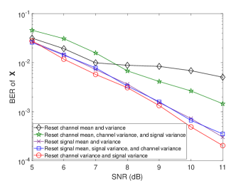
(a) BER of $\mathbf{X}$

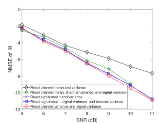
(b) NMSE of $\mathbf{H}$

Figure 3: The performance comparison of different re-initialization methods, where $M=M^{{}^{\prime}}=128$, $K=20$, $N=N^{{}^{\prime}}=1$, $T=100$, $\rho=0.1$, and $\lambda=0.1$.

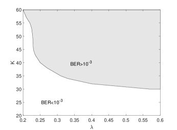
(a) $\rho=0.4$

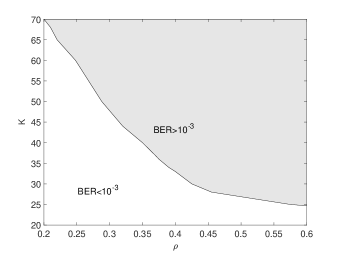
(b) $\lambda=0.4$

Figure 4: The phase transition of the BCSE scheme for the model in (20), where $M=M^{{}^{\prime}}=128$, $N=N^{{}^{\prime}}=1$, and $T=256$.

Fig. 4 shows the requirements on $K$, $\rho$, and $\lambda$ for successful recovery with other parameters fixed at $M=M^{{}^{\prime}}=128$, $N=N^{{}^{\prime}}=1$, $T=256$, and SNR $=20$ dB. We say that the recovery is successful and the corresponding value of $K$, $\rho$, and $\lambda$ are feasible if the BER of $\mathbf{X}<10^{-3}$. Fig. 4(a) shows the feasiable region of $(K,\lambda)$ with the signal sparsity $\rho=0.4$. We see that the boundary is a monotonic function of the sparsity level $\lambda$, i.e., the sparser the channel is, the greater the number of users can be supported. It is also interesting to see that the system is able to perform successful recovery with $K=30$, even for a relatively large $\lambda$. In this case, the user signals are still separable due to the signal sparsity. Fig. 4(b) shows the available region of $(K,\rho)$ with the channel sparsity $\lambda=0.4$. We observe that the boundary is also a monotonic function of the sparsity level $\rho$, as expected.

Fig. 5 shows the blind detection performance versus SNR, where $M=M^{{}^{\prime}}=128$, $N=N^{{}^{\prime}}=1$, $K=30$, $T=256$, $\rho=0.4$, and $\lambda=\lambda_{S}=0.1$. $T_{\rm P}=1+\lceil\log_{4}30\rceil$ QPSK symbols are used as pilots for each packet. For blind detection schemes, these pilots are used to remove phase and permutation ambiguities. From Fig. 5, we see that the BiG-AMP method only exploiting the signal sparsity in (12a) does not work well, neither does the training-based method. The BCSE for (19) has obvious performance loss than the BCSE for (20) since a loss of constellation constraints. The BiGAMP for (1) suffers from an error floor due to the unavoidable energy leakage problem of using the DFT basis for grid sampling. Clearly, our proposed BCSE algorithm significantly outperforms the counterpart schemes. Also, the proposed BCSE algorithm approaches the genie bound in the high SNR regime.

The proposed BCSE algorithm can also compare with the other bilinear recovery algorithm, such as BAd-VAMP in [32] and PBIGAMP in [18]. However, these algorithms will have high complexity in the settings in Fig. 5, so we try to compare in a small setup. We reset simulation settings as $M=M^{{}^{\prime}}=32$, $N=N^{{}^{\prime}}=4$, $K=1$, $T=50$, $\rho=0.2$, and $\lambda=0.2$. From Fig. 6, we see that BAd-VAMP and PBiGAMP do not work well. The proposed BCSE algorithm considerably outperforms BAd-VAMP and PBiGAMP.

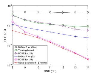
(a) BER of $\mathbf{X}$

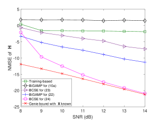
(b) NMSE of $\mathbf{H}$

Figure 5: $M=M^{{}^{\prime}}=128$, $N=N^{{}^{\prime}}=1$, $K=30$, $T=256$, $\rho=0.4$, and $\lambda=\lambda_{S}=0.1$.

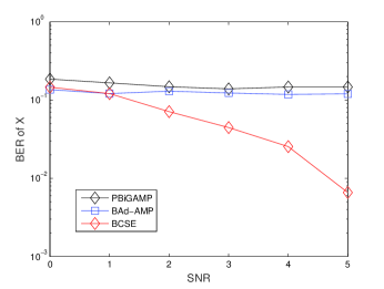
Figure 6: BER Performance of different schemes in a small setup, where $M\!=\!M^{{}^{\prime}}\!=\!32$, $K=1$, $N\!=\!N^{{}^{\prime}}\!=\!4$, $T\!=\!50$, $\rho\!=\!0.2$, and $\lambda\!=\!0.2$.

VI-B Performance of Semi-Blind Channel-and-Signal Estimation

We still assume that the true AoAs generated by (40) and the AoA grid perfectly covers the true AoAs. A uniform sampling grid is adopted to generate the AoDs, i.e., $\mathbf{A}_{\textsf{T,k}}(\bm{\varphi}_{k})$ is a DFT matrix for each user $k$. The parameter settings are $M=M^{{}^{\prime}}=128$, $N=N^{{}^{\prime}}=8$, $K=3$, $T=100$, $\rho=0.3$, and $\lambda=0.1$. Fig. 7 shows the BER performance versus SNR for various schemes with the number of pilots $T_{\rm P}=$ 4 and 8. From Fig. 7, we see that the SBCSE method for $T_{\rm P}=4$ significantly outperforms the training-based scheme and BiGAMP for (1). The SBCSE scheme outperforms the BCSE scheme by about 1 dB at BER $=10^{-4}$ for $T_{\rm P}=8$. We also see that, as in contrast to Fig. 5, there is a performance gap of about 1 dB between the SBCSE scheme and the genie bound with $\mathbf{S}$ known in the relatively high SNR regime. This is caused by the suboptimal estimation for $\mathbf{G}$ using the iterative soft-thresholding algorithm.

We extend our algorithms to the LAA antenna array, with the corresponding steering vectors given by

$$\mathbf{a}_{\textsf{R}}(\theta_{k}) =\left[\textrm{sinc}\!\left(-\frac{M^{{}^{\prime}}-1}{2}-\frac{D}{\varrho}\sin\theta_{k}\!\right),\textrm{sinc}\!\left(-\frac{M^{{}^{\prime}}-3}{2}-\frac{D}{\varrho}\sin\theta_{k}\!\right),\cdots,\textrm{sinc}\left(\frac{M^{{}^{\prime}}-1}{2}-\frac{D}{\varrho}\sin\theta_{k}\right)\right]^{T}$$

$$\mathbf{a}_{\textsf{T}}(\phi_{k}) =\left[\textrm{sinc}\left(-\frac{N^{{}^{\prime}}-1}{2}-\frac{D}{\varrho}\sin\phi_{k}\right),\textrm{sinc}\left(-\frac{N^{{}^{\prime}}-3}{2}-\frac{D}{\varrho}\sin\phi_{k}\right),\cdots,\textrm{sinc}\left(\frac{N^{{}^{\prime}}-1}{2}-\frac{D}{\varrho}\sin\phi_{k}\right)\right]^{T},$$ (41)

where $\textrm{sinc}(\cdot)$ denotes the nominalized “sinc” function, and $D$ denotes the lens length along the azimuth plane. We have added the simulation results in the LAA antenna geometry in Fig. 8. We see a similar performance trend in Fig. 8 as the case of ULA in Fig. 7.

We further study the impact of large-scale fading on the system performance. The channel powers $v_{\rm pri}$ of the $k$-th user are randomly drawn from a uniform distribution over $[v_{\rm pri,\rm min},1]$. Figure. 9 shows the performance of the various schemes in the presence of large-scale fading. In simulations, we set $-10\log 10(v_{\rm pri,\rm min})=20$ dB, and the EM algorithm in Section V is employed for the tuning of of $v_{\rm pri}$. The other settings are the same as those in Fig. 7. From Fig. 9, we see that the trends of the curves are very similar to those in Fig. 7.

Fig. 10 shows the transition diagrams for the BCSE and SBCSE schemes, where $M=M^{{}^{\prime}}=128$, $T=100$, $T_{\rm P}=8$, $KN=24$, $N=N^{{}^{\prime}}$, $\lambda=0.1$, and SNR $=20$ dB. Clearly, for fixed $KN$, $\lambda_{S}$ increases monotonically with $N$, or in other words, decreases with $K$. We see SBCSE works well in a much broader region of the channel and the signal sparsity than BCSE does.

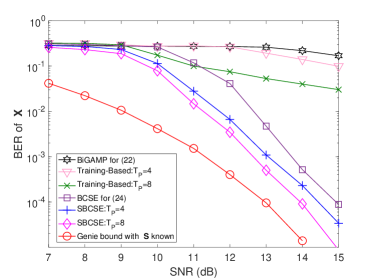
Figure 7: BER Performance of different schemes with $M\!=\!M^{{}^{\prime}}\!=\!128$, $K=3$, $N\!=\!N^{{}^{\prime}}\!=\!8$, $T\!=\!100$, $\rho\!=\!0.3$, and $\lambda\!=\!0.1$.

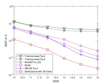
Figure 8: BER Performance of different schemes under LAA, where $M\!=\!M^{{}^{\prime}}\!=\!128$, $K=3$, $N\!=\!N^{{}^{\prime}}\!=\!8$, $T\!=\!100$, $\rho\!=\!0.3$, and $\lambda\!=\!0.1$.

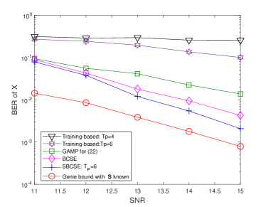
Figure 9: BER Performance of different schemes in large-scale fading, where $M\!=\!M^{{}^{\prime}}\!=\!128$, $K=3$, $N\!=\!N^{{}^{\prime}}\!=\!8$, $T\!=\!100$, $\rho\!=\!0.3$, and $\lambda\!=\!0.1$.

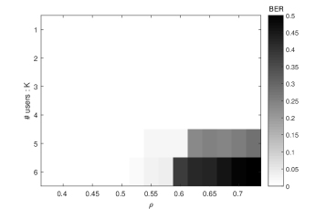
(a) BCSE

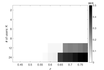
(b) SBCSE

Figure 10: Phase transition diagrams for BCSE and SBCSE without parameter tuning, where $M=M^{{}^{\prime}}=128$, $KN=24$, $T=100$, $T_{\rm P}=8$, and SNR $=20$ dB.

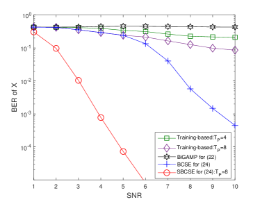
Figure 11: Performance of different schemes with parameter tuning, where $M=M^{{}^{\prime}}=128$, $T=100$, $T_{\rm P}=8$, $K=3$, $N=N^{{}^{\prime}}=8$, and $\rho=0.35$.

VI-C BCSE and SBCSE with Parameter Learning

We now assume that the AoAs are unknown to the BS. The channel is generated by the model in (9). Specially, we generate the center angle of each scattering cluster uniformly from $[-\frac{\pi}{2},\frac{\pi}{2}]$, and the AoA of each subpath $\theta(i,j)$ concentrates in a $20^{\circ}$ angular spread. $L_{1,c}=\cdots=L_{K,c}=3$ and $L_{1,p}=\cdots=L_{K,p}=50$. For the AoDs, we assume that $\{\phi_{k}(i,j)\}$ fall on a uniform sampling grid in the virtual angular domain. Fig. 11 shows the BER performance against SNR with $M=M^{{}^{\prime}}=128$, $T=100$, $T_{\rm P}=8$, $K=3$, $N=N^{{}^{\prime}}=8$, and $\rho=0.35$. The Markov chain model in (24) is used for characterising the clustering effect of the channel. The parameters in $\bm{\psi}$ are tuned using the EM method in Section V-A. Similar trends as in Fig. 7 has been observed in Fig. 11. Particularly, the SNR gap between SBCSE ($T_{\rm P}=8$) and BCSE is enlarged to over $5$ dB at BER $=10^{-3}$.

We further add the experiment in the spatial channel model (SCM) developed in 3GPP/3GPP2 for low frequency band (less than 6 GHz) [33]. The parameters of SCM used in the simulations are listed in Table. III. Fig. 12 shows the BER performance of different schemes against SNR with $M=M^{{}^{\prime}}=128$, $T=100$, $T_{\rm P}=8$, $K=1$, $N=N^{{}^{\prime}}=8$, and $\rho=0.4$.

TABLE III: Parameter Settings for the Channel Model

Parameter Settings for the SCM
Parameter name	Value	Parameter name	Value
Scenario	‘urban$\_$macro’	CenterFrequency	2GHz
NumBsElements	128	NumMsElements	8
NumPaths	3	NumSubPathsPerPath	20

From Fig. 12, we see that the BiGAMP method does not work well, neither does the training-based method. The BCSE with AoAs and AoDs tuning outperforms the BCSE without angles tuning. Further, we see that the SBCSE scheme with AoAs and AoDs tuning considerably outperforms the BCSE scheme for $T_{\rm P}$= 8.

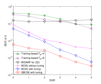
Figure 12: BER Performance of different schemes in SCM channel model, where $M\!=\!M^{{}^{\prime}}\!=\!128$, $K=1$, $N\!=\!N^{{}^{\prime}}\!=\!8$, $T\!=\!100$, $\rho\!=\!0.4$.

VII Conclusions

In this paper, we have studied joint antenna activity detection, channel estimation, and multiuser detection for massive MIMO system with GSM. We first designed the BCSE algorithm by exploiting the double-sparsity of the system model. We further developed the SBCSE algorithm, where a short pilot sequence is first used to estimate the phase and permutation ambiguities and then compressed sensing is adopted to enhance the estimation performance. Extensive numerical results have been provided to demonstrate the superior performance of the proposed BCSE and SBCSE algorithms over the state-of-the-art blind detection and training-based algorithms.

References

- [1] X. Kuai, X. Yuan, W. Yan, H. Liu, and Y. Zhang, “Sparsity learning based blind signal detection for massive MIMO with generalized spatial modulation,” in Proc. of the IEEE International Conference on Communications in China (ICCC), Aug. 2019.
- [2] G. Li, Z. Xu, C. Xiong, C. Yang, S. Zhang, Y. Chen, and S. Xu, “Energy-efficient wireless communications: Tutorial, survey, and open issues,” IEEE Wireless Commun., vol. 18, no. 6, pp. 28–35, Dec. 2011.
- [3] E. Björnson, L. Sanguinetti, J. Hoydis, and M. Debbah, “Optimal design of energy-efficient multi-user MIMO systems: Is massive MIMO the answer?” IEEE Trans. Wireless Commun., vol. 14, no. 6, pp. 3059–3075, Jun. 2015.
- [4] M. Renzo, H. Haas, and P. Grant, “Spatial modulation for multiple-antenna wireless systems: A survey,” IEEE Commun. Mag., vol. 49, no. 12, Dec. 2011.
- [5] N. Naidoo, H. Xu, and T. Quazi, “Spatial modulation: Optimal detector asymptotic performance and multiple-stage detection,” IET Commun., vol. 5, no. 10, pp. 1368–1376, 2011.
- [6] F. Rusek, D. Persson, B. Lau, E. Larsson, T. Marzetta, O. Edfors, and F. Tufvesson, “Scaling up MIMO: Opportunities and challenges with very large arrays,” IEEE Signal Process. Mag., vol. 30, no. 1, pp. 40–60, Jan. 2013.
- [7] T. Narasimhan, P. Raviteja, and A. Chockalingam, “Generalized spatial modulation in large-scale multiuser MIMO systems,” IEEE Trans. Wireless Commun., vol. 14, no. 7, pp. 3764–3779, Jul. 2015.
- [8] J. Zheng, “Low-complexity detector for spatial modulation multiple access channels with a large number of receive antennas,” IEEE Commun. Lett., vol. 18, no. 11, pp. 2055–2058, Nov. 2014.
- [9] C. Xu, S. Sugiura, S. Ng, and L. Hanzo, “Spatial modulation and space-time shift keying: Optimal performance at a reduced detection complexity,” IEEE Trans. Commun., vol. 61, no. 1, pp. 206–216, Jan. 2013.
- [10] A. Younis, S. Sinanović, R. Di, R. Mesleh, and H. Haas, “Generalised sphere decoding for spatial modulation,” arXiv preprint arXiv:1305.1478, 2013.
- [11] W. Liu, N. Wang, M. Jin, and H. Xu, “Denoising detection for the generalized spatial modulation system using sparse property,” IEEE Commun. lett., vol. 18, no. 1, pp. 22–25, May 2014.
- [12] T. Narasimhan, P. Raviteja, and A. Chockalingam, “Large-scale multiuser SM-MIMO versus massive MIMO,” in 2014 Information Theory and Applications Workshop (ITA). IEEE, 2014, pp. 1–9.
- [13] G.-R. Adrian and M. Christos, “Low-complexity compressive sensing detection for spatial modulation in large-scale multiple access channels,” IEEE Trans. Commun., vol. 63, no. 7, pp. 2565–2579, Dec. 2015.
- [14] S. Wang, Y. Li, and J. Wang, “Multiuser detection in massive spatial modulation MIMO with low-resolution ADCs,” IEEE Trans. Wireless Commun., vol. 14, no. 4, pp. 2156–2168, Apr. 2015.
- [15] D. L. Donoho, “Compressed sensing,” IEEE Trans. Inf. Theory, vol. 52, no. 4, pp. 1289–1306, 2006.
- [16] Y. Zhou, M. Herdin, A. Sayeed, and E. Bonek, “Experimental study of MIMO channel statistics and capacity via the virtual channel representation,” Univ. Wisconsin-Madison, Madison, WI, USA, Tech. Rep, vol. 5, pp. 10–15, 2007.
- [17] L. Chen, A. Liu, and X. Yuan, “Structured turbo compressed sensing for massive MIMO channel estimation using a Markov prior,” IEEE Trans. Veh. Technol., vol. 67, no. 5, May 2018.
- [18] J. Parker and P. Schniter, “Parametric bilinear generalized approximate message passing,” IEEE J. Sel. Topics Signal Process., vol. 10, no. 4, pp. 795–808, Jun. 2016.
- [19] H. Liu, X. Yuan, and Y.-J. A. Zhang, “Super-resolution blind channel-and-signal estimation for massive mimo with arbitrary array geometry,” IEEE Trans. Signal Process., vol. 67, no. 17, pp. 4433–4448, Sep. 2019.
- [20] J. Zhang, X. Yuan, and Y. Zhang, “Blind signal detection in massive MIMO: Exploiting the channel sparsity,” IEEE Trans. Communi., vol. 66, no. 2, pp. 7820–7830, Feb. 2017.
- [21] T. Ding, X. Yuan, and S. C. Liew, “Sparsity learning based multiuser detection in grant-free massive-device multiple access,” IEEE Transactions on Wireless Communications, pp. 1–1, 2019.
- [22] C.-K. Wen, C.-J. Wang, S. Jin, K.-K. Wong, and P. Ting, “Bayes-optimal joint channel-and-data estimation for massive MIMO with low-precision ADCs,” IEEE Trans. Signal Process., vol. 64, no. 10, pp. 2541–2556, May 2016.
- [23] J. Dai, L. An, and V. K. Lau, “FDD massive MIMO channel estimation with arbitrary 2D-array geometry,” IEEE Trans. Signal Process., vol. 66, no. 10, pp. 2584–2599, May 2018.
- [24] A. Liu, L. Lian, V. Lau, and X. Yuan, “Downlink channel estimation in multiuser massive MIMO with hidden markovian sparsity,” IEEE Trans. Signal Process., vol. 66, no. 18, pp. 4796–4810, Sep. 2018.
- [25] M. Aharon, M. Elad, and A. Bruckstein, “K-SVD: An algorithm for designing overcomplete dictionaries for sparse representation,” IEEE Trans. Signal Process., vol. 54, no. 11, pp. 4311–4322, Nov. 2006.
- [26] J. Mairal, F. Bach, J. Ponce, and G. Sapiro, “Online learning for matrix factorization and sparse coding,” J. Mach. Learn. Res., vol. 11, pp. 19–60, Jan. 2010.
- [27] D. Spielman, H. Wang, and J. Wright, “Exact recovery of sparsely-used dictionaries,” in JMLR: Workshop and Conference Proceedings, 2012, pp. 1–18.
- [28] J. Parker, P. Schniter, and V. Cevher, “Bilinear generalized approximate message passing Part I: Derivation,” IEEE Trans. Signal Process., vol. 62, no. 22, pp. 5839–5853, Nov. 2014.
- [29] J. Sun, Q. Qu, and J. Wright, “Complete dictionary recovery over the sphere I: Overview and the geometric picture,” IEEE Trans. Inf. Theory, vol. 63, no. 2, pp. 853–884, Feb. 2017.
- [30] S. Rangan, “Generalized approximate message passing for estimation with random linear mixing,” in Proc. of 2011 IEEE Int. Symp. on Inf. Theory (ISIT), St. Petersburg, Russia, 31 Jul.-5 Aug. 2011.
- [31] S. Wright, R. Nowak, and M. Figueiredo, “Sparse reconstruction by separable approximation,” IEEE Trans. Signal Process., vol. 57, no. 7, pp. 2479–2493, Jul. 2009.
- [32] S. Sarkar, A. K. Fletcher, S. Rangan, and P. Schniter, “Bilinear recovery using adaptive vector-amp,” IEEE Trans. Signal Process, vol. 67, no. 13, pp. 3383–3396, July 2019.
- [33] J. Salo, G. Del Galdo, J. Salmi, P. Kyösti, M. Milojevic, D. Laselva, and C. Schneider. (2005, Jan.) MATLAB implementation of the 3GPP Spatial Channel Model (3GPP TR 25.996). [Online]. Available: http://www.tkk.fi/Units/Radio/scm/