Axisymmetric spheroidal squirmers and self-diffusiophoretic particles

Abstract

We study, by means of an exact analytical solution, the motion of a spheroidal, axisymmetric squirmer in an unbounded fluid, as well as the low Reynolds number hydrodynamic flow associated to it. In contrast to the case of a spherical squirmer — for which, e.g., the velocity of the squirmer and the magnitude of the stresslet associated with the flow induced by the squirmer are respectively determined by the amplitudes of the first two slip (“squirming”) modes — for the spheroidal squirmer each squirming mode either contributes to the velocity, or contributes to the stresslet. The results are straightforwardly extended to the self-phoresis of axisymmetric, spheroidal, chemically active particles in the case when the phoretic slip approximation holds.

I Introduction

Self-propulsion of micro-organisms, such as bacteria, algae and protozoa, plays an important role in many aspects of nature. Whether a bacteria tries to reach a nutrient rich area or a sperm cell an unfertilized egg, motility often yields a substantial advantage over competitors. Due to their small size and velocity, the viscous friction experienced by the micro-organisms swimming in water is very strong compared to inertial forces pedley1992hydrodynamic ; guasto2012fluid ; consequently, they have developed swimming mechanisms adapted to these circumstances.

The motion of motile bacteria and other small organisms is typically induced by the beating of thin, thread-like appendages, the so called flagella; however, these species exhibit a broad morphology, in that they may posses either a single flagellum (e.g., monotrichous bacteria), several flagella (e.g., E. coli.), or a carpet of many small flagella, called cilia (e.g. Opalina). Focusing for the moment on the example of cilia covered micro-organisms, it was proposed by Lighthill that the emergence of motility can be understood without a detailed modeling of the complex, synchronous beating of the cilia lighthill1952squirming . Instead, the effect of this beating pattern, i.e., the time-averaged surface flow induced by the envelope of cilia tips, has been modeled as providing a prescribed active flow velocity $\mathbf{v}$ (actuation) at the surface of the particle (both within the tangent plane of the surface, $\mathbf{v}_{s}$, and in the direction normal to the surface, $\mathbf{v}_{n}$). The model, known by now as the “squirmer” model, was subsequently corrected and extended by his student Blake blake1971spherical .

In its simplest and most used form, the tangential slip velocity of a spherical squirmer is taken to be the superposition of the fore-aft asymmetric and fore-aft symmetric modes with the slowest decaying contributions to flow in the surrounding liquid, i.e., the leading order modes. Combined, they make for a squirmer endowed with motility (from the leading fore-aft asymmetric mode) and with a hydrodynamic stresslet (from the leading fore-aft symmetric mode) zottl2014hydrodynamics ; gotze2010mesoscale ; zhu2012self ; uspal2015rheotaxis ; wang2012inertial .

Considerable progress has already been made in understanding the behavior of spherical squirmers, and many interesting questions have been answered, such as: what does the flow field around a squirmer look like and how it compares with the ones produced by simple microorganisms blake1971spherical ; drescher2010direct ; downton2009simulation ; what happens if the swimmer is not in free space, but rather disturbed by boundaries zottl2014hydrodynamics or external flows uspal2015rheotaxis ; and how do pairs or even swarms of these particles interact gotze2010mesoscale . Although this model can also be used to better understand the motion of micro-organisms, e.g. Volvox pedley2016squirmers , observed in experiments, its restriction to spherical swimmers limits a wider application. For example, Paramecia, one of the most studied ciliates, has an elongated body sonneborn1970methods ; zhang2015paramecia ; ishikawa2006interaction , which prevents a straightforward application of the traditional squirmer model. However, the aforementioned questions are also of interest for these and other elongated micro-organisms. A generalization of the squirmer model to non-spherical shapes is thus a natural, useful development.

Driven by advances in technology that allow increasingly sophisticated manufacturing capabilities, in the last decade significant efforts have been made towards the development of artificial swimmers ismagilov2002autonomous ; ozin2005dream ; Faivre2017 ; ren2017rheotaxis ; golestanian2007designing . The envisioned lab-on-a-chip devices and micro-cargo carriers ebbens2010pursuit ; sundararajan2008catalytic , e.g., for targeted drug deliveries and nanomachines focused on monitoring and dissolving harmful chemicals soler2014catalytic ; gao2014environmental , all need to perform precise motions on microscopic length scales. A better understanding of the general framework of microscale locomotion is required in order to optimally design and control such devices, and theoretical models facilitate new steps along this path. As one example, chemically active colloids achieve self-propulsion by harvesting local free energy. They catalyze a chemical reaction in the surrounding fluid and propel due to the ensuing chemical gradient. Spherical “Janus” particles belong to this group, and it has been shown that the squirmer model can, in various circumstances, capture essential features of their motion Popescu2018 . However, there are many chemically active colloids with non-spherical shape, and rod-like particles are especially prevalent in experimental studies (see, e.g., Paxton2004 ; Paxton2006 ; ren2017rheotaxis ; mathijssen2018oscillatory ).

It is well known that passive, non-spherical colloids exposed to an ambient flow exhibit significant qualitative differences — such as alignment with respect to the direction of the ambient flow uspal2013engineering , Jeffery orbits by ellipsoids in shear flow jeffery1922motion , nematic ordering arising from steric repulsion lettinga2005flow , or noise-induced migration away from confining surfaces park2007cross — in comparison to their spherical counterparts. It is thus reasonable to expect that endowing such objects with a self-propulsion mechanism will lead to rich, qualitatively novel dynamical behaviors, some of which may be advantageous for, while others may hinder, applications. Accordingly, it is important to develop an in-depth understanding of the shape-dependent behavior, and significant experimental and theoretical efforts have been made in this direction (see, e.g., Refs. Kessler2004 ; Wensink2012 ; Goldstein2012 ; Frey2018 ; Dogic2017 ; Goldstein2016 ; Clement2015 ; DiLeonardo2017 ; DiLeonardo2018 ; Poon2018 as well as the insightful reviews provided in Refs. pedley1992hydrodynamic ; Powers2009 ; Ebbens2010 ; Gompper2015_rev ; Sen2010_rev ; Sagues_review_2018 ; Shelley2013 ; Ramaswamy2002 ; Bechinger2016_rev ).

Similar to the case of spherical swimmers, physical insight into the phenomenology exhibited by elongated swimmers can be gained from a corresponding squirmer model. For a model spheroidal swimmer moving by small deformations of its surface, Ref. felderhof2016stokesian derived an analytic solution to the corresponding Stokes flow, from which the velocity of the swimmer could be calculated. In Ref. leshansky2007frictionless it has been pointed out that an exact squirmer model for a spheroidal particle with a prescribed axi-symmetric, tangential slip velocity (active actuation of the fluid) on its surface can be written down by employing an available analytical solution for the axi-symmetric Stokes flow around a spheroidal object dassios1994generalized . However, the approach has been used in the context of a somewhat restricted model particle, involving an additional fore-aft asymmetry of the surface slip velocity, because of the particular interest, for that work, in the question of “hydrodynamically stealthy” microswimmers. While capturing the self-propulsion velocity of the swimmer, this removes certain characteristics of the flow, inter alia those that contribute to the corresponding stresslet lauga2016stresslets and would allow distinguishing between, e.g., “puller” and “pusher” type squirmers. Moreover, the particle stresslet is a key quantity connecting the microscopic dynamics of individual particles in a colloidal suspension with the continuum rheological properties of the suspension. For active particles like bacteria, the activity-induced stresslet can lead to novel material properties like ”superfluidity” and spontaneous flow Clement2015 .

We note that also a strongly truncated model, based on an ansatz for the slip velocity in the form of two terms which, in the corresponding limit of a sphere, reproduce the first two modes of the spherical squirmer model of Lighthill and Blake, has been discussed by Ref. theers2016modeling . This approach, however, is significantly affected by the fact that — as noticed in Ref. felderhof2016stokesian and also discussed here (see Sec. IV) — for spheroidal squirmers both their velocity and their stresslet involve significant contributions from the higher order slip modes, in contrast to the case of a spherical squirmer for which only the first two modes contribute to those observables.

In this paper we employ the available analytical solution for axi-symmetric Stokes flow around a spheroidal object dassios1994generalized to study the velocity and the induced hydrodynamic flow field around a spheroidal squirmer with a tangential slip velocity possessing axial symmetry, but otherwise unconstrained. The model squirmer is introduced in Sec. II. The series representation of the incompressible, axi-symmetric, creeping flow field around a spheroid dassios1994generalized is succinctly summarized in Sec. III. In Section IV we discuss the velocity and the flow field corresponding to the spheroidal squirmer, with particular emphasis on illustrating the contributions from the modes of various order. Additionally, in Sec. IV.1 we discuss the straightforward extension of these results to deriving the flow field around a chemically active self-phoretic spheroid (for a similar mapping in the case of spherical particles see Ref. Michelin2014 ). The final Sect. V is devoted to a summary of the results and to the conclusions of the study.

II Model

The model system we consider is that of a spheroidal, rigid and impermeable particle immersed in an incompressible, unbounded, quiescent Newtonian liquid through which it moves due to a prescribed “slip velocity” (active actuation) at its surface (see Fig. 1). The slip velocity $\mathbf{v}_{s}$, which is tangential to the surface $\Sigma$ of the particle (i.e., $\mathbf{n}\cdot\mathbf{v}_{s}\equiv 0$ on $\Sigma$, with $\mathbf{n}$ denoting the outer (into the fluid) normal to $\Sigma$), is assumed to preserve the axial symmetry and to be constant in time, but it is otherwise arbitrary. The surface slip $\mathbf{v}_{s}$ is part of the model and thus it is a given function (or, alternatively as in, c.f., Sec. IV.1, it is determined as the solution of a separate problem). There are no external forces or torques acting on either the particle or the liquid.

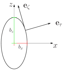
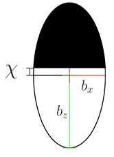
Figure 1: (a) Two-dimensional (2d) cut of a prolate spheroidal particle with semi-major axis $b_{z}$ and semi-minor axis $b_{x}$; also shown are the $x$ and $z$ axes of the co-moving system of coordinates and the unit vectors $\mathbf{e}_{\tau}$ and $\mathbf{e}_{\zeta}$ of the prolate spheroidal coordinate system; (b) 2d cut of a chemically-active self-phoretic particle; the chemically active part is the cap-like region shown in white, while the rest of the surface (black) is chemically inert. The quantity $\chi$ (“coverage”) denotes a certain measure for the extent of the active part (see Sec. IV.1 in the main text).

Due to the surface actuation, a hydrodynamic flow around the particle is induced and the particle sets in motion; we assume that the linear size $L$ of the particle, the viscosity $\mu$ and the density $\varrho$ of the liquid, and the magnitude $|\mathbf{v}_{s}|$ of the slip velocity are such that the Reynolds number $\mathrm{Re}:=\varrho|\mathbf{v}_{s}|L/\mu$ is very small. Accordingly, after a short transient time a steady state hydrodynamic flow is induced around the particle and the particle translates steadily with velocity $\mathbf{U}$ (with respect to a fixed system of coordinates, the “laboratory frame”). (Owing to the axial symmetry, in the absence of thermal fluctuations, which are neglected in this work, there is no rigid-body rotation of the particle in this model.)

The analysis is more conveniently carried out in a system of coordinates attached to the particle (co-moving system). This is chosen with the origin at the center of the particle and such that the $z$-axis is along the axis of symmetry of the particle (thus $\mathbf{U}=U\mathbf{e}_{z}$). The semi-axis of the particle are accordingly denoted by $b_{z}$ and $b_{x}$ (see Fig. 1); their ratio $r_{e}=\frac{b_{x}}{b_{z}}$ is called the aspect ratio and determines the slenderness of the particle. The values $r_{e}<1$, $r_{e}=1$, and $r_{e}>1$ correspond to prolate, spherical, and oblate shapes, respectively.

In the co-moving system of coordinates, the flow $\mathbf{v}$ and the velocity $\mathbf{U}$ are determined as the solution of the Stokes equations

$$\nabla\cdot\boldsymbol{\sigma}=0\,,~{}~{}\nabla\cdot\mathbf{v}=0\,,$$ (1)

where

$$\boldsymbol{\sigma}:=-p\,\mathcal{I}+\mu[\nabla\mathbb{v}+(\nabla\mathbb{v})^{T}]\,,$$ (2)

is the Newtonian stress tensor, with $p$ denoting the pressure (enforcing incompressibility), $\mathcal{I}$ denoting the unit tensor, and $()^{T}$ denoting the transpose, subject to:
– the boundary conditions (BC)

$$\mathbb{v}|_{\Sigma}=\mathbb{v}_{s}\,,$$ (3a)

and

$$\mathbb{v}(|\mathbb{r}|\to\infty)\rightarrow-\mathbb{U}\,.$$ (3b)

– the force balance condition (overdamped motion of the particle in the absence of external forces)

$$\int\limits_{\Sigma}\boldsymbol{\sigma}\cdot\mathbb{n}\,d\Sigma=0\,.$$ (4)

The hydrodynamic flow $\mathbb{v}_{\mathrm{lab}}$ in the laboratory frame, if desired, is then obtained as $\mathbb{v}_{\mathrm{lab}}(\mathrm{P})=\mathbb{v}(\mathrm{P})+\mathbb{U}$, with $\mathrm{P}$ denoting the observation point.

The boundary-value problem above can be straightforwardly solved numerically by using, e.g., the Boundary Element Method (BEM) (see, e.g., Refs. ishimoto2017guidance ; uspal2015rheotaxis ; katuri2018cross ; Simmchen2016 ) as well as analytically. In the following, we shall focus on the analytical solution of this problem; the corresponding numerical solutions obtained by the BEM are presented in Appendix .5 and used as a means of testing the convergence of the series representation of the analytical solution. Before proceeding, we note that we will focus the discussion on the case of prolate shapes, i.e., $r_{e}<1$ (see Fig. 1(a)); the case of an oblate squirmer ($r_{e}>1$) can be obtained from the results for the prolate shapes via a certain mapping (see, e.g., Ref. leshansky2007frictionless and Appendix .1), while the case of a sphere is obtained from the results corresponding to a prolate spheroid by taking the limit $r_{e}\to 1^{-}$.

III Hydrodynamic flow and velocity of a prolate squirmer

The calculation of the hydrodynamic flow $\mathbb{v}$ induced by the squirmer and of the velocity $\mathbb{U}$ of the squirmer are most conveniently carried out by employing the modified prolate spheroidal coordinates $(1\leq\tau\leq\infty,-1\leq\xi\leq 1,0\leq\phi\leq 2\pi)$ as in Ref. dassios1994generalized . These are defined in the co-moving system of reference, which has the origin in the center of the particle, and are related to the Cartesian coordinates via dassios1994generalized

$$\tau=\frac{1}{2c}(\sqrt{x^{2}+y^{2}+(z+c)^{2}}+ \sqrt{x^{2}+y^{2}+(z-c)^{2}}\large{)}\,,$$

$$\zeta=\frac{1}{2c}(\sqrt{x^{2}+y^{2}+(z+c)^{2}}- \sqrt{x^{2}+y^{2}+(z-c)^{2}}),$$ (5)

$$\varphi=\arctan \left(\frac{y}{x}\right)\,,$$

where $c=\sqrt{b_{z}^{2}-b_{x}^{2}}$ is a purely geometric quantity which ensures smooth convergence into spherical coordinates in the limit $b_{x}\rightarrow b_{z}$. The unit vectors $\mathbf{e}_{\tau}$ and $\mathbf{e}_{\zeta}$ (see Fig. 1) are related to the ones of the Cartesian coordinates via

$$\mathbb{e}_{\tau} = \left(\frac{2\tau\cdot\sqrt{1-\zeta^{2}}}{\sqrt{\tau^{2}-1}}\mathbb{e}_{x}+\zeta\mathbb{e}_{z}\right)\cdot\frac{\sqrt{\tau^{2}-1}}{\sqrt{\tau^{2}-\zeta^{2}}}\,,$$

$$\mathbb{e}_{\zeta} = \left(\frac{2\zeta\cdot\sqrt{\tau^{2}-1}}{\sqrt{1-\zeta^{2}}}\mathbb{e}_{x}+\tau\mathbb{e}_{z}\right)\cdot\frac{\sqrt{1-\zeta^{2}}}{\sqrt{\tau^{2}-\zeta^{2}}}\,,$$ (6)

and the corresponding Lamé metric coefficients are given by

$$h_{\zeta}=c\frac{\sqrt{\tau^{2}-\zeta^{2}}}{\sqrt{1-\zeta^{2}}}\,,$$

$$h_{\tau}=c\frac{\sqrt{\tau^{2}-\zeta^{2}}}{\sqrt{\tau^{2}-1}}\,,$$ (7)

$$h_{\varphi}=c\sqrt{\tau^{2}-1}\sqrt{1-\zeta^{2}}\,.$$

The iso-surfaces $\tau=const$ are confocal prolate spheroids with common center $\mathrm{O}$; the surface of the particle corresponds to

$$\tau_{0}=\frac{b_{z}}{c}=\frac{1}{\sqrt{1-r_{e}^{2}}}>1\,,$$ (8)

and the values $\tau>\tau_{0}$ ($1\leq\tau<\tau_{0}$) correspond to the exterior (interior) of the prolate ellipsoid, respectively. The coordinate $\zeta$ takes the values $\zeta=\pm 1$ at the $z=\pm b_{z}$ apexes, respectively, and $\zeta=0$ on the equatorial ($x-y$ plane cut) circle. Note that, as shown in Fig. 1(a), $\mathbb{e}_{\tau}$ coincides with the normal $\mathbf{n}$ while $\mathbf{e}_{\zeta}$ and $\mathbf{e}_{\phi}$ span the tangent plane.

III.1 Velocity of the squirmer

The velocity of the squirmer can be determined from Eqs. (1) - (4) as a linear functional of the axi-symmetric slip velocity $\mathbb{v}_{s}=v_{s}(\zeta)\mathbb{e}_{\zeta}$ without explicitly solving for the flow $\mathbb{v}$. This follows via a straightforward application of the Lorentz reciprocal theorem (happel2012low, , Chapter 3-5). For the case of the prolate spheroid with $\mathbb{U}=U\mathbb{e}_{z}$, this renders (for details see, e.g., Refs. leshansky2007frictionless ; popescu2010phoretic ; lauga2016stresslets )

$$U=-\frac{\tau_{0}}{2}\int\limits^{1}_{-1}\text{d}\zeta\,\sqrt{\frac{1-\zeta^{2}}{\tau_{0}^{2}-\zeta^{2}}}\,v_{s}(\zeta)\,.$$ (9)

Therefore, $\mathbb{U}$ can be considered as known; accordingly, the boundary value problem defined by Eqs. (1) - (4) is specified and the solution $\mathbb{v}$ can be determined.

III.2 Stokes stream function and hydrodynamic flow

Since the boundary value problem defined by Eqs. (1) - (3) has axial symmetry, one searches for an axisymmetric solution $\mathbb{v}(\mathbb{r})$ expressed in terms of a Stokes stream function $\psi(\mathbb{r})$ as $\mathbb{v}(\mathbb{r})=\nabla\times\frac{\psi(\mathbb{r})}{h_{\varphi}}\mathbb{e}_{\varphi}$ (happel2012low, , Chapter 4); this renders

$$v_{\tau}(\tau,\zeta) =\frac{1}{h_{\zeta}h_{\varphi}}\frac{\partial\psi}{\partial\zeta}\,,$$ (10)

$$v_{\zeta}(\tau,\zeta) =-\frac{1}{h_{\tau}h_{\varphi}}\frac{\partial\psi}{\partial\tau}.$$ (11)

The general “semiseparable” solution for the stream function in prolate coordinates has been derived by Ref. dassios1994generalized in the form of a series representation

$$\psi(\tau,\zeta) =g_{0}(\tau)G_{0}(\zeta)+g_{1}(\tau)G_{1}(\zeta)$$

$$+\sum_{n=2}^{\infty}[g_{n}(\tau)G_{n}(\zeta)+h_{n}(\tau)H_{n}(\zeta)].$$ (12)

where $G_{n}$ and $H_{n}$ are the Gegenbauer functions of the first and second kind, respectively (see Ref. Abramowitz ). The functions $g_{n}(\tau)$ and $h_{n}(\tau)$ are given by certain linear combinations of $G_{k}(\tau)$ and $H_{k}(\tau)$, the coefficients of which are fixed by the corresponding boundary conditions (see below).

The general solution above is applied to our particular system as follows. Noting that for our system the solution $\mathbb{v}(\mathbb{r})$ should be bounded (i.e., $|\mathbb{v}(\mathbb{r})|<\infty$ everywhere), none of the terms involving the Gegenbauer functions of the second kind $H_{n}(\zeta)$, which are divergent along the $z$-axis (i.e., $\zeta=\pm 1$) (happel2012low, , Chapter 4-23), can be present in the solution; accordingly, $h_{n}(\tau)\equiv 0$ for all $n\geq 2$. Furthermore, due to the same requirement of bounded magnitude of the flow, the terms involving the Gegenbauer functions of the first kind $G_{0}(\zeta)=1$ and $G_{1}(\zeta)=-\zeta$ also cannot be present in the solution because they lead to divergences of $v_{\zeta}$ at $\zeta=\pm 1$ (see Eqs. (11) and (III)); accordingly, $g_{0}(\tau)\equiv 0$ and $g_{1}(\tau)\equiv 0$. Therefore, for our system only the functions $g_{n\geq 2}$ will be of interest; these are given by dassios1994generalized

$$g_{2}(\tau)= \frac{C_{2}}{6}G_{1}(\tau)+C_{4}H_{4}(\tau)+D_{2}H_{2}(\tau)$$

$$+F_{2}G_{2}(\tau)+E_{4}G_{4}(\tau)$$

$$g_{3}(\tau)= -\frac{C_{3}}{90}G_{0}(\tau)+C_{5}H_{5}(\tau)+D_{3}H_{3}(\tau)$$ (13)

$$+F_{3}G_{3}(\tau)+E_{5}G_{5}(\tau)$$

$$g_{n\geq 4}(\tau)= C_{n+2}H_{n+2}(\tau)+C_{n}H_{n-2}(\tau)+D_{n}H_{n}(\tau)$$

$$+F_{n}G_{n}(\tau)+E_{n+2}G_{n+2}(\tau)+E_{n}G_{n-2}(\tau),$$

where the constants $\{C_{n},D_{n}\}_{n\geq 2}$, $\{E_{n}\}_{n\geq 4}$, and $\{F_{n}\}_{n\geq 2}$, are fixed, as noted above, by requiring that the solution satisfies the BCs, Eqs. (3), and the force balance condition, Eq. (4).

Since the hydrodynamic force is proportional to the coefficient $C_{2}$ (see $g_{2}(\tau)$) leshansky2007frictionless , the force balance (Eq. (4)) implies

$$C_{2}=0\,.$$ (14a)

The boundary condition at infinity (Eq. (3b)) implies the asymptotic behavior of the stream function

$$\psi(\tau\to\infty,\zeta)\propto\frac{1}{2}Uc^{2}(\tau^{2}-1)(1-\zeta^{2})\,;$$

by noting the asymptotic behaviors $$G_{n}(\tau\gg 1)\propto\tau^{n} H_{n}(\tau\gg 1)\propto\tau^{-(n+1)} g_{n\geq 2}(\tau) G_{n}(\tau) n>2$$ and Abramowitz , this implies that the functions cannot have contributions from terms involving the Gegenbauer functions of index , i.e.,

$$E_{n}=0\,,~{}n=4,5,\dots~{}~{}\mathrm{and}~{}~{}F_{n}=0\,,n=3,4,\dots$$ (14b)

Furthermore, in order to exactly match the asymptotic $$(\tau^{2}-1)(1-\zeta^{2})$$ form and its prefactor, it is necessary that

$$F_{2}=-2c^{2}U\,.$$ (14c)

The impenetrability of the surface and Eq. (10) imply that $$\psi(\tau_{0},\zeta) \psi(\tau_{0},\pm 1)=0 G_{n}(\zeta=\pm 1)=0 \psi(\tau_{0},\zeta)\equiv 0$$ is a constant; since as , one concludes that and thus

$$g_{n}(\tau_{0})=0,~{}n=2,3,\dots$$ (14d)

Finally, the tangential slip velocity condition at the surface of the particle (Eq. (3a)) together with: the expression for $$v_{\zeta} G_{n\geq 2}(\zeta) G_{n\geq 2}(\zeta) P_{n\geq 1}^{1}(\zeta)$$ in Eq. (11), the orthogonality of the Gegenbauer functions (see Appendix .2), and the relation between the Gegenbauer functions and the associated Legendre polynomials (see the Appendix 30) leads to

$$\left.\frac{dg_{n}}{d\tau}\right|_{\tau=\tau_{0}}= c^{2}(n-\frac{1}{2})\int\limits_{-1}^{+1}\mathrm{d}\zeta(\tau_{0}^{2}-\zeta^{2})^{1/2}v_{s}(\zeta)P_{n-1}^{1}(\zeta)\,,$$

$$~{}n=2,3,\dots.$$ (14e)

For given $v_{s}(\zeta)$, and with $U$ determined by Eq. (9), Eqs. (14d) and (14) provide a system of linear equations determining all the remaining unknown coefficients $\{C_{n\geq 3},D_{n\geq 2}\}$, as detailed in the Appendix .3.

IV Squirmer and squirming modes

The form of Eq. (14) suggests (for the expansion of the slip velocity $\mathbf{v}_{s}$) the functions

$$V_{n}(\zeta):=(\tau_{0}^{2}-\zeta^{2})^{-1/2}P_{n}^{1}(\zeta)\,,$$ (15)

as a suitable basis over the space of square integrable functions $f(\zeta)$ satisfying $f(\zeta=\pm 1)=0$ (note that $V_{n}$ has a parametric dependence on $\tau_{0}>1$). Defining, in this space, the weighted scalar product

$$\langle f_{1}(\zeta),f_{2}(\zeta)\rangle_{w(\zeta)}:=\int\limits_{-1}^{+1}\mathrm{d}\zeta w(\zeta)f_{1}(\zeta)f_{2}(\zeta)\,,$$ (16)

and choosing the weight as

$$w(\zeta)=\tau_{0}^{2}-\zeta^{2}>0\,,$$ (17)

one infers (form the known properties of the associated Legendre polynomials) that indeed the set $\{V_{n}\}_{n\geq 1}$ is an orthogonal basis,

$$\langle V_{n}(\zeta),V_{m}(\zeta)\rangle_{w(\zeta)}=\frac{n(n+1)}{n+1/2}\delta_{n,m}\,.$$ (18)

Accordingly, the slip velocity function $\mathbb{v}_{s}=v_{s}(\zeta)\mathbb{e}_{\zeta}$ has a unique representation in terms of a series in the functions $\{V_{n}\}_{n\geq 1}$,

$$v_{s}(\zeta)=\tau_{0}\sum\limits_{n\geq 1}B_{n}V_{n}(\zeta)\,.$$ (19)

The coefficients of the expansion are written in the form above to ensure that in the limit of a sphere ($b_{x}\to b_{z}$, i.e, $\tau_{0}\to\infty$) one arrives at the usual form employed for a spherical squirmer, i.e., that of an expansion in associated Legendre polynomials $P_{n}^{1}(\cos\vartheta)$ (see, e.g., Ref. blake1971spherical ; ishikawa2008coherent ). This can be seen by noticing that in the limit $\tau_{0}\to\infty$ one has $\tau_{0}(\tau_{0}^{2}-\zeta^{2})^{-1/2}P_{n}^{1}(\zeta)\to P_{n}^{1}(\zeta)$ and that $b_{x}\to b_{z}$ implies $\zeta\to\cos(\vartheta)$; accordingly, it follows that, in the limit of the shape approaching that of a sphere, $\tau_{0}V_{n}(\zeta)\mathbf{e}_{\zeta}\to-P_{n}^{1}(\cos\vartheta)\mathbf{e}_{\vartheta}$ and the expansion in Ref. blake1971spherical is matched identically upon changing $B_{n}\rightarrow\frac{2}{n(n+1)}B_{n}$.

With the representation of the slip velocity in terms of the function $V_{n}$, Eq. (19), upon exploiting the orthogonality relation (Eq. (18)) the boundary condition in Eq. (14) renders the simple relations

$$\left.\frac{\partial g_{n}(\tau)}{\partial\tau}\right|_{\tau=\tau_{0}} =\tau_{0}c^{2}n(n-1)B_{n-1}\,,~{}n=2,3,\dots$$ (20)

For a given slip velocity, thus a given set of amplitudes $B_{n}$ of the slip modes $V_{n}(\zeta)$, Eqs. (14d) and (20) evaluated for $n\geq 1$ provide a system of coupled linear equations for the last unknown coefficients in the stream function, $C_{n\geq 3}$ and $D_{n\geq 2}$. Inspection of this system reveals that it splits into two subsystems of coupled equations, one involving only the coefficients of even index, $n=2k$, and the other one involving only the coefficients of odd index $n=2k+1$ (see Appendix .3). Furthermore, from Eq. (20) it can be inferred that in the case that the slip velocity is given by a pure slip mode $V_{n_{0}}(\zeta)$, i.e., $B_{n}=\delta_{n,n_{0}}$ for $n\geq 1$, then the parity of $n_{0}$ selects one of the two subsystems. If $n_{0}$ is even, then all the coefficients $C_{k}$ and $D_{k}$ of even index $k$ vanish and the stream function, Eq. (12), involves only the functions $g_{k}$ of odd index $k$, while for odd $n_{0}$ all the coefficients $C_{k}$ and $D_{k}$ of odd index $k$ vanish and the stream function, Eq. (12), involves only the functions $g_{k}$ of even index $k$. Finally, we note that a pure slip mode $V_{n_{0}}(\zeta)$ selects, as discussed above, either the odd or even number terms in the series representation of the the stream function, Eq. (12), but not only a single squirmer mode, as it is the case for the spherical squirmer. Accordingly, even simple distributions of active slip velocities on the surface of the particle can give rise to quite complex hydrodynamic flows around the squirmer.

With these general results, we can proceed to the discussion of prolate squirmers. We will focus on the usual quantities employed to characterize an axisymmetric squirmer lighthill1952squirming ; blake1971spherical ; felderhof2016stokesian , i.e., the velocity $U$ of the squirmer, the magnitude $S$ of the stresslet associated with the squirmer (which determines the far-field hydrodynamic flow of the squirmer), and the general characteristics of the hydrodynamic flow $\mathbf{v}(\mathbf{r})$ around the squirmer.

By combining Eqs. (14), (19), (18), and (15), and noting that the polynomials $P_{n}^{1}(x)$ are even (odd) functions of $x$ for $n$ odd (even), one arrives at

$$U(\tau_{0}) =\frac{\tau_{0}^{2}}{2}\sum_{n\geq 1,n~{}\mathrm{odd}}B_{n}\int\limits_{-1}^{1}dx\frac{P_{1}^{1}(x)P_{n}^{1}(x)}{\tau_{0}^{2}-x^{2}}$$ (21)

$$=\sum_{n\geq 1,n~{}\mathrm{odd}}B_{n}U_{n}(\tau_{0})\,.$$

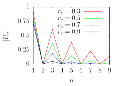
Figure 2: The absolute value $|U_{n}|$ (Eq. (21)) of the contribution of the slip modes $n=1,3,5,7$ to the velocity of a prolate squirmer for aspect ratios $r_{e}=0.3,0.5,0.7,0.9$. The lines represent only a guide to the eye.

Accordingly, it follows that (a) a squirmer may exhibit self-motility (i.e., $U\neq 0$) only if the slip velocity involves at least an odd index $n$ slip mode $V_{n}$; (b) in contrast to the case of a spherical squirmer, for which the velocity is determined solely by the slip mode $n=1$ irrespective of the details of the slip velocity $\mathbf{v}_{s}$, for a spheroidal squirmer all the slip modes of odd index contribute to the velocity (see also Fig. 2); consequently, (c) spheroidal squirmers with $B_{1}=0$ can be self-motile (due to contributions from other odd index slip modes), and spheroidal squirmers with $B_{1}\neq 0$ can yet be non-motile if the contributions from other slip modes of odd index $n$ precisely balance the contribution of the mode $B_{1}$ (which clearly pinpoints the shortcomings of a model with only two slip modes as in Ref. theers2016modeling ).

In terms of the dependence on the slenderness parameter $r_{e}$ (which determines the value of $\tau_{0}$, see Eq. (8)), there are two findings. (d) for every slip mode $n$, the contribution $|U_{n}|$ (in absolute value) is a decreasing function of $r_{e}$ (see Fig. 2); second, (e) while at low values of the aspect ratio the contributions $|U_{n}|$ of the $n>1$ slip modes are significant, the contributions from the modes $n\geq 3$ decay steeply with increasing $r_{e}$ and become negligible, compared to $|U_{1}|$ (which remains non-zero), as the aspect ratio $r_{e}$ of the spheroid approaches that of a sphere ($r_{e}\to 1^{-}$). This ensures a smooth transition into the spherical case, where, as previously mentioned, higher mode squirmers are not motile and $U\propto B_{1}$. Finally, we note that, by comparison with the expression in Eq. (14c), one infers that the series in the last line of Eq. (21) is proportional to the coefficient $F_{2}$ in the expansion of the stream function.

In what concerns the stresslet $S(\tau)$, which (similarly to the case of a spherical squirmer) allows classification into pullers (positive stresslet, $S>0$), pushers (negative stresslet, $S<0$), and neutral swimmers (vanishing stresslet, $S=0$), we note that it can also be expressed in terms of the slip velocity $u_{s}(\zeta)$ as lauga2016stresslets :

$$S =-\frac{2A\mu}{F(r_{e}^{-1})J(r_{e}^{-1})}\int^{1}_{-1}u_{s}(\zeta)\zeta\sqrt{\frac{r_{e}^{-2}(1-\zeta^{2})}{\zeta^{2}+r_{e}^{-2}(1-\zeta^{2})}}d\zeta$$ (22)

$$=\sum_{n\geq 1,n~{}\mathrm{even}}\mu B_{n}S_{n}(\tau_{0})$$

where $A$ denotes the surface area of the spheroid and

$$F(x)=\frac{1}{(x^{2}-1)^{2}}\left(-3x^{2}+\frac{x(1+2x^{2})}{\sqrt{1-x^{2}}}\cos^{-1}(x)\right),$$

$$J(x)=1+\frac{x^{2}}{\sqrt{x^{2}-1}}\cos^{-1}\left(\frac{1}{x}\right).$$

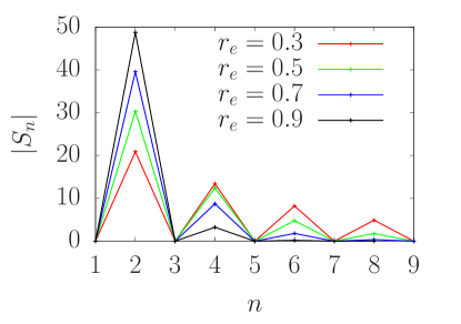
Figure 3: The absolute value $|S_{n}|$ (Eq. (22)) of the contribution of the slip modes $n=1,3,5,7$ to the stresslet of a prolate squirmer for aspect ratios $r_{e}=0.3,0.5,0.7,0.9$. The lines represent only a guide to the eye.

As in the case of the velocity, there are certain significant differences from the case of a spherical squirmer (see Fig. 3): (a) a necessary condition for a prolate squirmer to exhibit a nonvanishing stresslet is that at least one even ($k=2n$) mode $V_{k}$ contributes to the slip velocity; (b) as for the velocity $U$ (where more than a single mode contributes), the stresslet depends on all even squirmer modes; hence, (c) the stresslet contribution of $B_{2}\neq 0$ can be offset or even inverted by other even, active modes $B_{k}\neq 0$; (d) At a given aspect ratio $r_{e}$, the contribution (in absolute value) $|S_{2n}|$ is a decreasing function of $n$; and (e) while for elongated shapes (small values $r_{e}$) the contributions $|S_{n}|$ from the slip modes $n\geq 4$ are significant, these contributions are steeply decreasing towards zero with increasing $r_{e}$ towards the value $1^{-}$. In contrast, $|S_{2}|$ is increasing with $r_{e}$. As in the case of the velocity, this behavior ensures the smooth transition to the case of a spherical shape, where $S\propto B_{2}$.

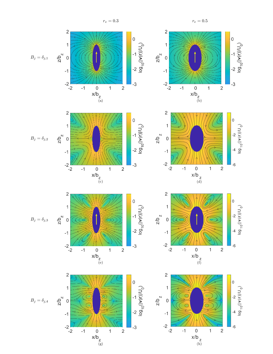
Figure 4: The flow field (streamlines and velocity magnitude (color coded background)) induced by a prolate squirmer with $B_{n}=\delta_{n,n_{0}}$ for (top to bottom) $n_{0}=1,2,3,4$ and aspect ratio $r_{e}=0.3$ (left column) and $r_{e}=0.5$ (right column), respectively. The results are shown in the laboratory frame and are obtained by using the series representation of the stream function (see the main text). The arrows on the particles indicate the directions of their motion.

Since the stresslet is, by definition, the amplitude of the $r^{-2}$ far-field term in the flow field (in the lab frame) of the squirmer, the series in the last line of Eq. (22) can be connected with one of the coefficients in the expansion of the stream function as follows. In the laboratory frame, which is related to the one ($\psi_{\text{particle}}$) in the co-moving frame via

$$\psi_{\text{lab}}=\psi_{\text{particle}}+\frac{1}{2}U_{0}(1-r_{e}^{2})(\tau^{2}-1)(1-\zeta^{2})\,,$$ (23)

the slowest decaying term with the distance $\tau$ from the squirmer is $-\frac{C_{3}}{90}\text{G}_{0}(\tau)\text{G}_{3}(\zeta)$; by Eq. (10), this term leads to a contribution $\sim C_{3}/\tau^{2}$ to the flow. Accordingly, $S\propto C_{3}$ and the pusher or puller squirmers ($S\neq 0$) indeed exhibit the expected far-field hydrodynamics, while for the neutral squirmers ($S=0$) the far-field flow necessarily decays at least as $\sim 1/\tau^{3}$.

Turning now to the flow field around the prolate squirmer, we will discuss separately the flow fields generated by the first few pure slip modes, i.e., the cases $B_{n}=\delta_{n,n_{0}}$ with $n_{0}=1,2,3,4$; these flows are shown, in the laboratory frame, in Fig. 4. From the discussion above, we know that only a subset (either the odd index ones, if $n_{0}$ is even, or vice versa) of the terms in the series representation, Eq. (12), of the stream functions contributes to the flow. Since the metric factors are even functions of $\zeta$, while $G_{n}(\zeta)$ is an odd (even) function of $\zeta$ when $n$ is odd (even), the flow has the following fore-aft symmetries. For $n_{0}$ odd, the stream function involves the functions $G_{k}$ of index $k$ an even number, and thus $\psi(\tau,\zeta)=\psi(\tau,-\zeta)$; this implies $v_{\tau}(\tau,\zeta)=-v_{\tau}(\tau,-\zeta)$ and $v_{\zeta}(\tau,\zeta)=v_{\zeta}(\tau,-\zeta)$ (see figures 5 and 6); i.e., the $z-$ ($x-$) flow components are fore-aft (anti)symmetric (see Fig. 4), and, accordingly, it contributes to the motility because it provides a “fore to back” streaming. Vice versa, for $n_{0}$ an even number one has $v_{\tau}(\tau,\zeta)=v_{\tau}(\tau,-\zeta)$ and $v_{\zeta}(\tau,\zeta)=-v_{\zeta}(\tau,-\zeta)$, i.e., the $x-$ ($z-$) flow component are fore-aft symmetric (see Fig. 4); consequently, they cannot be associated to a motile particle.

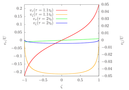
Figure 5: Velocity components $v_{\tau}$ and $v_{\zeta}$ on the iso-surfaces $\tau=1.1\tau_{0}$ and $\tau=2\tau_{0}$ near a prolate squirmer with $B_{n}=\delta_{n,1}$.

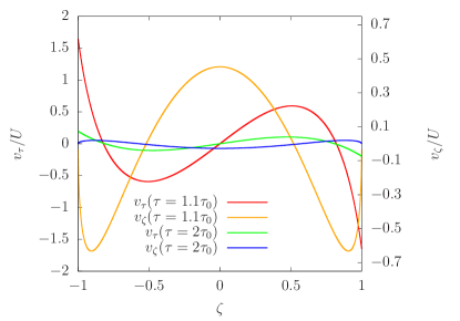
Figure 6: Velocity components $v_{\tau}$ and $v_{\zeta}$ on the iso-surfaces $\tau=1.1\tau_{0}$ and $\tau=2\tau_{0}$ near a prolate squirmer with $B_{n}=\delta_{n,3}$.

Finally, we note that the similar analysis and results for the case of an oblate squirmer can be obtained from the available ones for a prolate squirmer via a simple transformation of the coordinates system and of the stream function (i.e., a mapping), as discussed in the Appendix .1. As an illustration of using this mapping, the results shown in Fig. 4, corresponding to a prolate squirmer, have been used to determine the flows around the corresponding (i.e., of slenderness parameters $r^{\prime}_{e}=1/r_{e}$) oblate squirmers induced by the pure slip modes $B_{n}=\delta_{n,n_{0}}$ with $n_{0}=1,2,3,4$; these are shown in Fig. 7. The analysis of the velocity $U$ and stresslet $S$ (see Figs. 8 and 9) for oblate spheroids leads to conclusions that are similar with those drawn in the case of prolate shapes. The only significant difference is that now for oblate squirmers the contributions of from the higher orders $n$ slip modes decay to zero with decreasing aspect ratio $r_{e}\to 1^{+}$; again, this ensures a smooth transition to the case of a spherical shape, where only $B_{1}$ or $B_{2}$ are relevant.

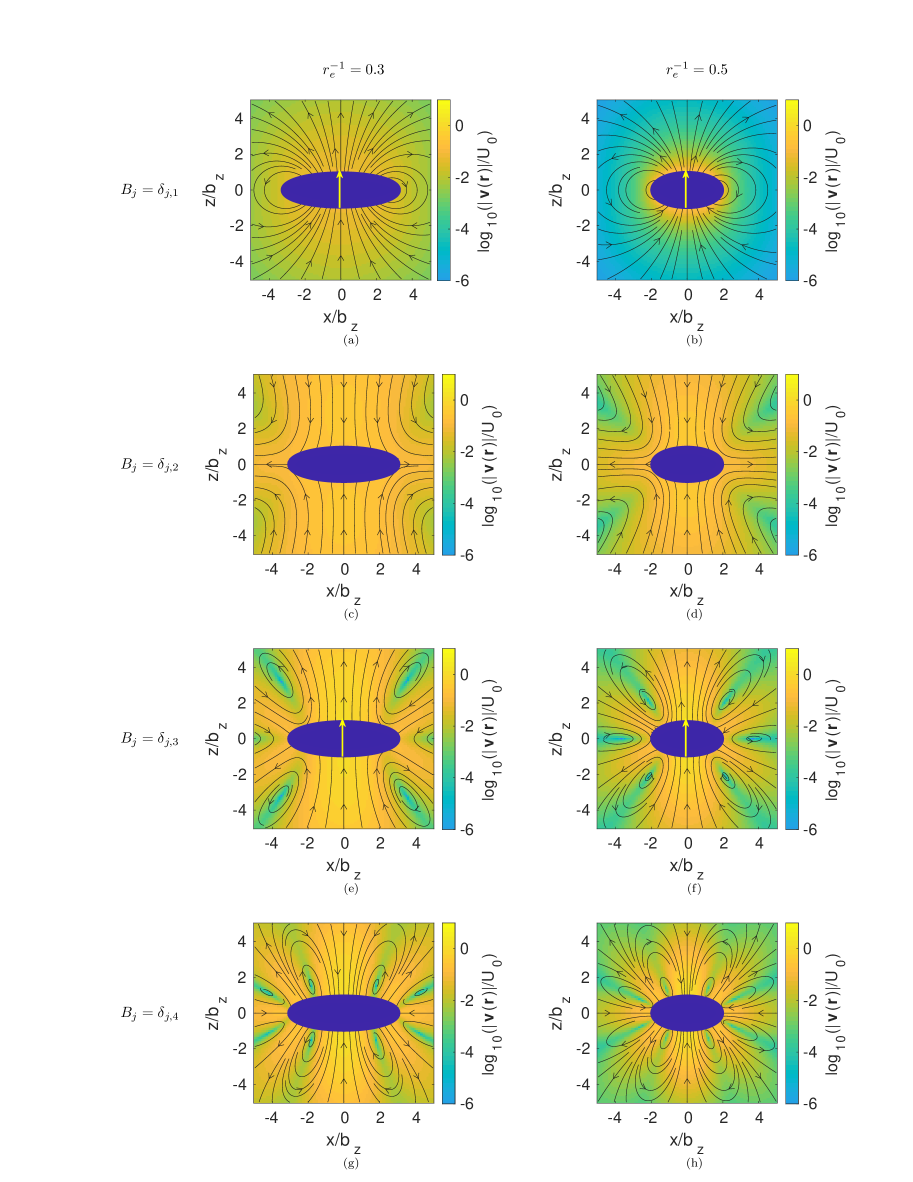
Figure 7: The flow field (streamlines and velocity magnitude (color coded background)) induced by an oblate squirmer with $B_{n}=\delta_{n,n_{0}}$ for (top to bottom) $n_{0}=1,2,3,4$ and aspect ratio $r_{e}^{-1}=0.3$ (left column) and $r_{e}^{-1}=0.5$ (right column), respectively. The results are shown in the laboratory frame and are obtained by using the mapping discussed in the main text and the flows of the corresponding prolate squirmers shown in Fig. 4. The arrows on the particles indicate the directions of their motion.

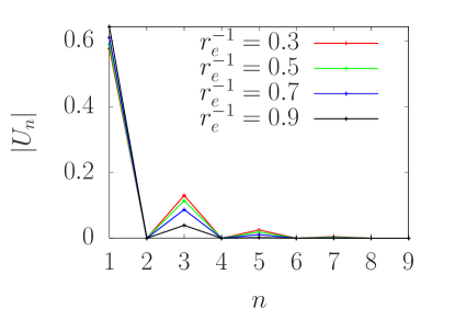
Figure 8: The absolute value $|U_{n}|$ of the contribution of the slip modes $n=1,3,5,7$ to the velocity of an oblate squirmer for aspect ratios $r_{e}^{-1}=0.3,0.5,0.7,0.9$. The lines represent only a guide to the eye.

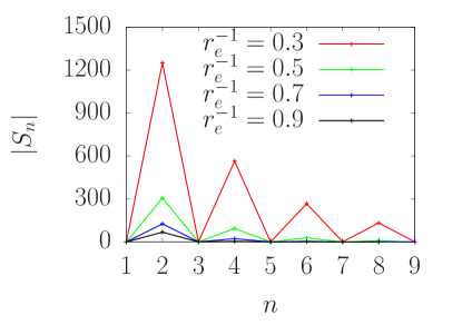
Figure 9: The absolute value $|S_{n}|$ of the contribution of the slip modes $n=1,3,5,7$ to the stresslet of an oblate squirmer for aspect ratios $r_{e}^{-1}=0.3,0.5,0.7,0.9$. The lines represent only a guide to the eye.

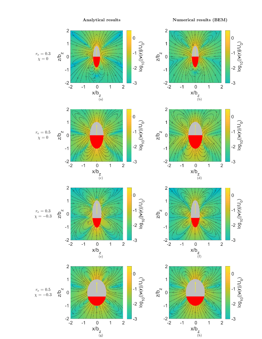
Figure 10: The flow field (streamlines and velocity magnitude (color coded background)) induced by a chemically active prolate particle moving by self-phoresis, calculated either analytically via the stream function (left column) or numerically, i.e., by directly solving the corresponding Laplace and Stokes equations using the BEM BEM (right). The results shown correspond to the cases of half ($\chi=0$, top two rows) and less than half ($\chi=-0.3$, bottom two rows) coverage, and two values, $r_{e}=0.3$ and $r_{e}=0.5$, of the aspect ratio, respectively. The arrows on the particles indicate the directions of their motion. The red area depicts the chemically active region. The motion of the particle and the direction of the flow corresponds to the choice $b<0$; the characteristic velocity $U_{0}$ is defined as in Ref. popescu2010phoretic

IV.1 Self-phoretic particle

Squirmers with a wide range of active slip modes occur naturally in the context of model self-phoretic particles. One of the often employed realizations of such systems consists of micrometer-sized silica or polystyrene spherical particles partially coated with a Pt layer and immersed in an aqueous peroxide solution Howse2007 ; Baraban2012 ; Simmchen2016 . The catalytic decomposition of the peroxide at the Pt side creates gradients in the chemical composition of the suspension; as in the case of classic phoresis anderson1989colloid , these gradients, in conjunction with the interaction between the colloid and the various molecular species in solution, give rise to self-phoretic motility Golestanian2005 . The mechanism of steady-state motility can be intuitively understood in terms of the creation of a so-called phoretic slip velocity tangential to the surface of the particle golestanian2007designing ; anderson1989colloid ; Derjaguin1966 . For such chemically active, axi-symmetric, spherical particles in unbounded solutions, the approximation of phoretic slip velocity leads to a straightforward mapping Michelin2014 ; Popescu2018 onto a squirmer model; accordingly, the translational velocity of the particle and the hydrodynamic flow around the particle in terms of the phoretic slip can be directly inferred from the corresponding results in Ref. blake1971spherical .

A similar mapping can be developed from a spheroidal, self-phoretic colloid to a spheroidal squirmer model for spheroidal, chemically active colloids. Following Ref. popescu2010phoretic the slip velocity of such particles can be written as

$$v_{\text{S}}(\mathbb{r}_{\text{P}})=\sum_{l\geq 0}\frac{b}{c}c_{l}(\chi)\text{Q}_{l}(\tau_{0})\text{P}^{1}_{l}(\zeta)(\tau_{0}^{2}-\zeta^{2})^{-\frac{1}{2}},$$ (24)

where $b$ is the so-called phoretic mobility (for simplicity, here assumed to be a constant) over the surface of the particle, and $\text{Q}_{l}(\tau)$ denotes the Legendre polynomial of the second kind Abramowitz . The coverage $\chi=h-1$ is defined in terms of the height of the active cap (measured, from the bottom apex, in units of $b_{z}$), i.e., $\chi=-1$ corresponds to a chemically inactive spheroid and $\chi=+1$ corresponds to all the surface being active. The coverage dependent coefficients $c_{l}(\chi)$ (see Ref. popescu2010phoretic ) describe the decoration of the surface of the particle by the chemically active element (e.g., Pt in the example discussed above) as an expansion in Legendre polynomials $\text{P}_{l}(\zeta)$. Knowledge of these parameters allows us to formulate a slip velocity boundary condition similar to (20), i.e.

$$\frac{\partial g_{n}(\tau)}{\partial\tau}\Big{|}_{\tau=\tau_{0}}=\tau_{0}c^{2}n(n-1)\tilde{B}_{n-1}\,;$$ (25)

by identifying the effective squirmer modes $\tilde{B}_{l}=\frac{b}{c\cdot\tau_{0}}c_{l}\text{Q}_{l}(\tau_{0})$, the desired mapping is achieved. As an illustration of this mapping, we show in Fig. 10 (left column) the flow fields for particles with parameters $r_{e}=0.3,0.5$ and $\chi=0,-0.3$, respectively, and compare with the corresponding results obtained by direct numerical solutions obtained using BEM BEM . (Note that, if necessary, the accuracy of the analytical estimate can be systematically improved simply by increasing the order of the truncation in the series expansion of the stream function (see the Appendix .4)).

V Summary and conclusion

We have studied in detail the most general axi-symmetric spheroidal squirmer and we have shown that, in analogy with the situation for spherical shapes Michelin2014 , model chemically active, self-phoretic colloids can be mapped onto squirmers. By using the semiseparable ansatz derived in Ref. dassios1994generalized for the stream function, and representing the active slip (squirming) velocity of the squirmer in a suitable basis (Eq. (19), chosen such that in the limit of a spherical shape it smoothly transforms into the usually employed expansion for the classical spherical squirmer blake1971spherical , the velocity of the squirmer, the stresslet of the squirmer, and the hydrodynamic flow around the squirmer have been determined analytically (Sec. IV). The corresponding series representations have been validated by cross-checking against direct numerical calculations, obtained by using the BEM, of the flow around the squirmer (Appendix .5).

The main conclusion emerging from the study is that for spheroidal squirmers (or self-phoretic particles) the squirming modes beyond the second are, in general, as important as the first two ones in what concerns the contributions to the velocity and stresslet of the particle (and, implicitly, to the flow field around the particle, even in the far-field). The velocity is contributed by all the odd-index components (but none of the even-index ones) of the slip velocity; accordingly, in contrast with the case of spherical squirmers, it is possible to have spheroidal squirmers with a non-zero first mode and yet not motile, as well as ones missing the first slip mode and yet motile. Similarly, the stresslet value is contributed by all the even-index slip modes; thus, distinctly from the case of spherical squirmers, one can have pushers/pullers even if the second slip mode is vanishing, as well as neutral squirmers in spite of a non-vanishing second slip mode. Finally, even a single slip mode leads to a large number of non-vanishing terms in the series expansion of the stream function, and thus spheroidal squirmers with simple distributions of slip on their surface can lead to very complex flows around them (see Figs. 4 and 7).

This raises the interesting speculative question as whether the spheroidal shape is providing an evolutionary advantage; i.e., with small modifications of the squirming pattern, e.g., switching from a sole $B_{1}$ mode to a sole $B_{3}$ mode, a microrganism could maintain its velocity unchanged but dramatically alter the topology of the flow around it (compare the first and third rows in Fig. 4). In other words, compared to a squirmer with spherical shape, for which multiple modes must be simultaneously activated in order to change the structure of the flow, a spheroidal squirmer possesses simple means for acting in hydrodynamic disguise, which can be advantageous as either predator or prey.

.1 Oblate spheroids

The similarity between oblate and prolate spheroids allows us to obtain the flow field around an oblate microswimmer of aspect ratio $r_{e}^{\prime}>1$ as a series in the oblate coordinates by using a mapping from the results, in prolate coordinates, corresponding to a prolate microswimmer with aspect ratio $r_{e}=1/r_{e}^{\prime}<1$ (and vice versa).

The oblate spheroidal coordinate system is defined by

$$\lambda=\frac{1}{2\bar{c}}(\sqrt{x^{2}+y^{2}+(z-i\bar{c})^{2}}+ \sqrt{x^{2}+y^{2}+(z+i\bar{c})^{2}}\large{)}\,,$$

$$\zeta=\frac{1}{-2i\bar{c}}(\sqrt{x^{2}+y^{2}+(z-i\bar{c})^{2}}- \sqrt{x^{2}+y^{2}+(z+i\bar{c})^{2}}),$$

$$\varphi=\arctan \left(\frac{y}{x}\right)\,,$$

with $0\leq\lambda\leq\infty$ and $\bar{c}=\sqrt{r_{e}^{\prime 2}-1}$, and the corresponding Lamé metric coefficients are given by

$$h_{\zeta}=\bar{c}\frac{\sqrt{\lambda^{2}+\zeta^{2}}}{\sqrt{1-\zeta^{2}}}\,,~{}~{}~{}h_{\lambda}=\bar{c}\frac{\sqrt{\lambda^{2}+\zeta^{2}}}{\sqrt{\lambda^{2}+1}}\,,$$ (26)

$$h_{\varphi}=\bar{c}\sqrt{\lambda^{2}+1}\sqrt{1-\zeta^{2}}\,.$$

Noting that the oblate coordinates and the metric factors can be obtained from the expressions of the corresponding prolate coordinates via the transformations dassios1994generalized

$$\tau\rightarrow i\lambda\qquad c\rightarrow-i\bar{c}\,,$$ (27)

one concludes that the equation and boundary conditions obeyed by the stream function in oblate coordinates in the domain outside the oblate of aspect ratio $r_{e}^{\prime}=1/r_{e}$ can be obtained, by using the same transformation, from the ones in prolate coordinates outside a prolate of aspect ratio $r_{e}$. Accordingly, it follows that $\psi_{\text{obl,$r_{e}^{\prime}=1/r_{e}$}}(\lambda,\zeta)=\psi_{\text{pro,$r_{e}$}}(\tau=i\lambda,\zeta)$. The flow field then follows as the curl of the stream function, i.e.,

$$\mathbb{v}_{\text{obl,$r_{e}^{\prime}$}}(\lambda,\xi,\varphi)=\nabla\times\left(\frac{\psi_{\text{obl,$r_{e}^{\prime}$}}(\lambda,\xi)}{h_{\varphi}}\,\,\mathbb{e}_{\varphi}\right).$$ (28)

.2 Gegenbauer functions

The Gegenbauer functions of first kind $G_{n}$, are also known as the Gegenbauer polynomials $C^{\alpha}_{n}$ with parameter $\alpha=-1/2$ Abramowitz ; they are defined in terms of the Legendre polynomials $P_{n}$ as

$$G_{n}(x)=\frac{1}{2n-1}\left(P_{n-2}(x)-P_{n}(x)\right)\;,$$ (29a)

and fulfill the orthogonality relation

$$\int_{-1}^{1}\frac{G_{n}(x)G_{m}(x)}{1-x^{2}}dx=\frac{2}{n(n-1)(2n-1)}\delta_{n,m}\quad n,m\geq 2\,.$$ (30)

The Gegenbauer functions can be related to the associated Legendre polynomials $\text{P}^{1}_{n}$, which are defined in terms of the Legendre polynomials $P_{n}$ as

$$(1-x^{2})^{1/2}\text{P}^{1}_{l}=-(1-x^{2})\frac{\text{d}}{\text{d}x}P_{l}(x).$$

Using the relations $\frac{x^{2}-1}{n}\frac{\text{d}}{\text{d}x}P_{n}(x)=x\text{P}_{n}(x)-\text{P }_{n-1}(x)$ and $(n+1)\text{P}_{n+1}(x)=(2n+1)x\text{P}_{n}(x)-n\text{P}_{n-1}(x)$, one arrives at the following relation between the $l$-th associated Legendre polynomial and the $l+1$-th Gegenbauer function.

$$(1-x^{2})^{1/2}\text{P}^{1}_{l}=-(l^{2}+l)\text{G}_{l+1}(x)$$

.3 Decoupling of the even- and odd-index modes in the stream function expansion

The coefficients $C_{n}$ and $D_{n}$ appear in the functions $g_{k}(\tau)$, entering the series expansion of the stream function at various indexes $k$ (e.g., $C_{n\geq 4}$ appears at both $k=n-2$ and $k=n$); thus the infinite system of linear equations is strongly coupled. However, since the even and odd terms are not entering the same equations, the system splits into two decoupled subsystems, which are solved by using different methods.

The first subsystem consists of the even numbered terms in the series expansion of $\psi(\tau,\zeta)$ and the set of conditions (Eqs. (14a), (14c), (14d) and (20)). Because each of the Eqs. (14a) and (14c) fix one of the even index coefficients (i.e., $C_{2}$ and $F_{2}$), the Eqs. (14d) and (20) evaluated at $n=2$ involve only two unknowns, $C_{4}$ and $D_{2}$, and thus can be solved as a sub-subsystem. With $C_{4}$ and $D_{2}$ known, the rest of the coefficients, up to the order $N_{max}$ at which the system is truncated (i.e., $B_{k}$ is set to zero for $k>N_{max}$), are solved iteratively by noting that Eqs. (14d) and (20) evaluated at $k=n$ involve only two unknowns, the rest of the coefficients being already determined in the previous iterations up to $k=n-2$.

The second subsystem includes all odd-index terms in the series expansion of $\psi(\tau,\zeta)$ and Eqs. (14d) and (20). Complementing the previous case, only the even squirmer modes contribute. However, unlike in the case of the first subsystem, there are no lower level decouplings; accordingly, this subsystem is solved in the standard manner by truncation at the cut-off $N_{max}$ (above which all the coefficients are set to zero) and inversion of the resulting finite system of linear equations.

The choice of $N_{max}$ is done by varying the value of the cut-off and testing the changes in the coefficients. For the cases we analyzed in this work, a value $N_{max}=16$ was found to be sufficient.

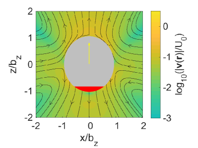
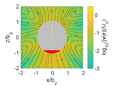
Figure 11: The flow field around a self-phoretic particle ($\chi=0.8$, $r_{e}=0.9$) when keeping the first (a) two and (b) eight terms (effective squirmer modes) in the series expansion of the stream function. The red area depicts the chemically active region.

.4 Example of effects of too strong truncations for the case self-phoretic particles

To show the importance of the higher orders in the case of a self-phoretic swimmer, we compare the analytic results for keeping different numbers of squirmer modes $B_{n}$ in figure 11. Even for an aspect ratio $r_{e}=0.8$ (i.e., close to a spherical shape), the higher orders have significant influence on the flow field around the particle: e.g., compare the occurrence of a region of high magnitude flow near the point $(0,-1.5)$ (behind the particle) instead of the correct location at near the point $(0,1.5)$ (in front of the particle).

.5 Quantitative comparison to BEM

In figures 12 - 14 we present a more detailed comparison of the results obtained by using the series representation (top row) with numerical results obtained by using the BEM to directly solve the governing equations (second row). In addition, the relative error, defined as

$$\Delta v=\frac{\sqrt{(v_{x,ana}-v_{x,num})^{2}+(v_{z,ana}-v_{z,num})^{2}}}{\frac{1}{2}(\sqrt{v_{x,ana}^{2}+v_{z,ana}^{2}}+\sqrt{v_{x,num}^{2}+v_{z,num}^{2}})}$$ (31)

is shown in the bottom row. The comparison confirms the expected quantitative agreement, with regions of significant relative error ($\Delta v>10^{-1}$) corresponding precisely to the regions where the flow is anyway very weak ($|\frac{\mathbb{v}/\mathbb{r})}{U}|<10^{-3}$).

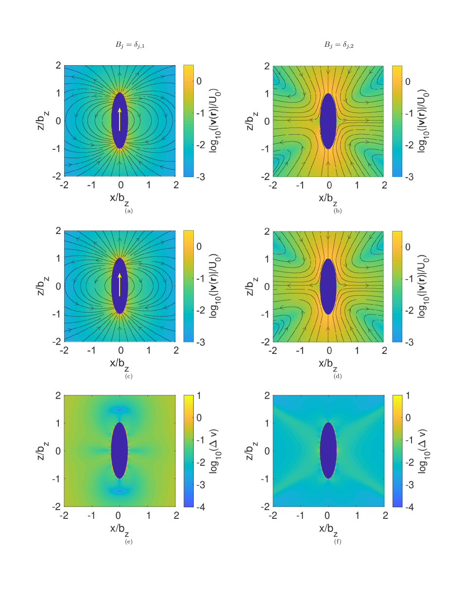
Figure 12: The flow field around a prolate squirmer with $r_{e}=0.3$; in the left column only the first slip mode is active, and on the right column only the second slip mode is active. In both cases the analytical results are shown in the top row, the numerical results (BEM BEM ) in the middle row, and the relative error between the two (Eq. (31)) in the bottom row.

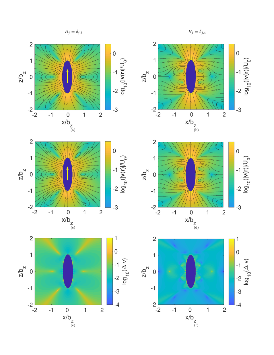
Figure 13: The flow field around a prolate squirmer with $r_{e}=0.3$; in the left column only the third slip mode is active, and on the right column only the fourth slip mode is active. In both cases the analytical results are shown in the top row, the numerical results (BEM BEM ) in the middle row, and the relative error between the two (Eq. (31)) in the bottom row.

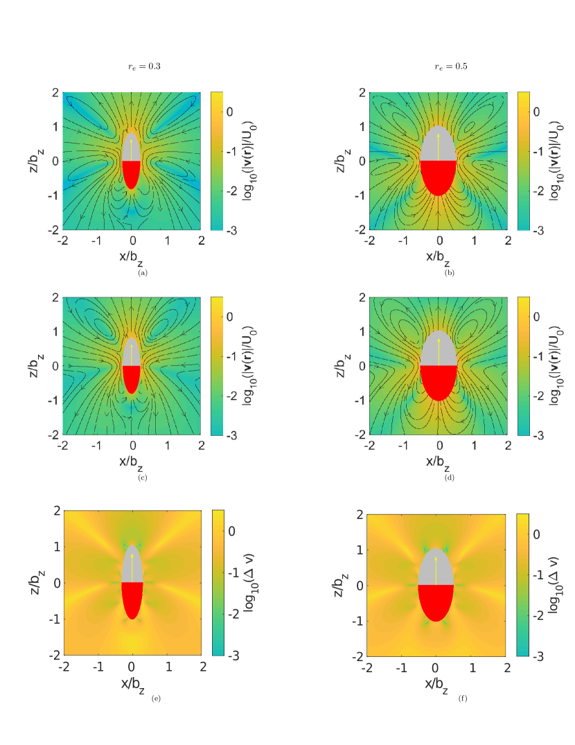
Figure 14: The flow field around half covered ($\chi=0$) self-phoretic particles with aspect ratio $r_{e}=0.3$ (left) and $r_{e}=0.5$ (right). In both cases the analytical results are shown in the top row, the numerical results (BEM BEM ) in the middle row, and the relative error between the two (Eq. (31)) in the bottom row. The red area depicts the chemically active region.

References

- (1) T.J. Pedley and J.O. Kessler. Hydrodynamic phenomena in suspensions of swimming microorganisms. Annual Review of Fluid Mechanics 24, 313–358 (1992).
- (2) J.S. Guasto, R. Rusconi, and R. Stocker. Fluid mechanics of planktonic microorganisms. Annual Review of Fluid Mechanics 44, 373–400 (2012).
- (3) M.J. Lighthill. On the squirming motion of nearly spherical deformable bodies through liquids at very small Reynolds numbers. Communications on Pure and Applied Mathematics 5, 109–118 (1952).
- (4) J.R. Blake. A spherical envelope approach to ciliary propulsion. Journal of Fluid Mechanics 46, 199–208 (1971).
- (5) A. Zöttl and H. Stark. Hydrodynamics determines collective motion and phase behavior of active colloids in quasi-two-dimensional confinement. Physical Review Letters 112, 118101 (2014).
- (6) I.O. Götze and G. Gompper. Mesoscale simulations of hydrodynamic squirmer interactions. Physical Review E 82, 041921 (2010).
- (7) L. Zhu, E. Lauga, and L. Brandt. Self-propulsion in viscoelastic fluids: Pushers vs. pullers. Physics of Fluids 24, 051902 (2012).
- (8) W.E. Uspal, M.N. Popescu, S. Dietrich, and M. Tasinkevych. Rheotaxis of spherical active particles near a planar wall. Soft Matter 11, 6613–6632 (2015).
- (9) S. Wang and A. Ardekani. Inertial squirmer. Physics of Fluids 24, 101902 (2012).
- (10) K. Drescher, R. E. Goldstein, N. Michel, M. Polin, and I. Tuval. Direct measurement of the flow field around swimming microorganisms. Physical Review Letters 105, 168101 (2010).
- (11) M. T. Downton and H. Stark. Simulation of a model microswimmer. Journal of Physics: Condensed Matter 21, 204101 (2009).
- (12) T. J. Pedley, D. R. Brumley, and R. E. Goldstein. Squirmers with swirl: a model for Volvox swimming. Journal of Fluid Mechanics 798, 165–186 (2016).
- (13) T.M. Sonneborn. Methods in Paramecium research. In Methods in cell biology, volume 4, pp. 241–339. Elsevier (1970).
- (14) P. Zhang, S. Jana, M. Giarra, PP. Vlachos, and S. Jung. Paramecia swimming in viscous flow. The European Physical Journal Special Topics 224, 3199–3210 (2015).
- (15) T. Ishikawa and M. Hota. Interaction of two swimming Paramecia. Journal of Experimental Biology 209, 4452–4463 (2006).
- (16) R.E. Ismagilov, A. Schwartz, N. Bowden, and G.M. Whitesides. Autonomous movement and self-assembly. Angewandte Chemie 114, 674–676 (2002).
- (17) G.A. Ozin, I. Manners, S. Fournier-Bidoz, and A. Arsenault. Dream nanomachines. Advanced Materials 17, 3011–3018 (2005).
- (18) P. J. Vach, D. Walker, P. Fischer, P. Fratzl, and D. Faivre. Pattern formation and collective effects in populations of magnetic microswimmers. Journal of Physics D 50, 11LT03 (2017).
- (19) L. Ren, D. Zhou, Z. Mao, P. Xu, T.J. Huang, and T.E. Mallouk. Rheotaxis of Bimetallic Micromotors Driven by Chemical–Acoustic Hybrid Power. American Chemical Society Nano 11, 10591–10598 (2017).
- (20) R. Golestanian, T.B. Liverpool, and A. Ajdari. Designing phoretic micro-and nano-swimmers. New Journal of Physics 9, 126 (2007).
- (21) S. J. Ebbens and J. R. Howse. In pursuit of propulsion at the nanoscale. Soft Matter 6, 726–738 (2010).
- (22) S. Sundararajan, P. E. Lammert, A. W. Zudans, V. H. Crespi, and A. Sen. Catalytic motors for transport of colloidal cargo. Nano letters 8, 1271–1276 (2008).
- (23) L. Soler and S. Sánchez. Catalytic nanomotors for environmental monitoring and water remediation. Nanoscale 6, 7175–7182 (2014).
- (24) W. Gao and J. Wang. The environmental impact of micro/nanomachines: a review. American Chemical Society Nano 8, 3170–3180 (2014).
- (25) M. N. Popescu, W. E. Uspal, Z. Eskandari, M. Tasinkevych, and S. Dietrich. Effective squirmer models for self-phoretic chemically active spherical colloids. European Physical Journal E 41, 145 (2018).
- (26) W.F. Paxton, K.C. Kistler, C.C. Olmeda, A. Sen, S.K.St. Angelo, Y.Y. Cao, T.E. Mallouk, P.E. Lammert, and V.H. Crespi. Catalytic nanomotors: Autonomous movement of striped nanorods. Journal of the American Chemical Society 126, 13424 (2004).
- (27) W. F. Paxton, S. Sundararajan, T. E. Mallouk, and A. Sen. Chemical locomotion. Angewandte Chemie International Edition 45, 5420–5429 (2006).
- (28) A. Mathijssen, N. Figueroa-Morale, G. Junot, E. Clement, A. Lindner, and A. Zöttl. Oscillatory surface rheotaxis of swimming E. coli bacteria. Nature Communications 10, 3434 (2019).
- (29) W. E. Uspal, H. B. Eral, and P. S. Doyle. Engineering particle trajectories in microfluidic flows using particle shape. Nature Communications 4, 2666 (2013).
- (30) G.B. Jeffery. The motion of ellipsoidal particles immersed in a viscous fluid. Proceedings of the Royal Society London A 102, 161–179 (1922).
- (31) M. P. Lettinga, Z. Dogic, H. Wang, and J. Vermant. Flow behavior of colloidal rodlike viruses in the nematic phase. Langmuir 21, 8048–8057 (2005).
- (32) J. Park, J. M. Bricker, and J. E. Butler. Cross-stream migration in dilute solutions of rigid polymers undergoing rectilinear flow near a wall. Physical Review E 76, 040801 (2007).
- (33) C. Dombrowski, L. Cisneros, S. Chatkaew, R. E. Goldstein, and J. O. Kessler. Self-concentration and large-scale coherence in bacterial dynamics. Physical Review Letters 93, 098103 (2004).
- (34) H. H. Wensink, J. Dunkel, S. Heidenreich, K. Drescher, R. E. Goldstein, H. Löwen, and J. M. Yeomans. Meso-scale turbulence in living fluids. Proceedings of the National Academy of Sciences of the United States of America 109, 14308–14313 (2012).
- (35) F. G. Woodhouse and R. E. Goldstein. Spontaneous circulation of confined active suspensions. Physical Review Letters 109, 168105 (2012).
- (36) L. Huber, R. Suzuki, T. Krüger, E. Frey, and A. R. Bausch. Emergence of coexisting ordered states in active matter systems. Science 361, 255 – 258 (2018).
- (37) K.-T. Wu, J. B. Hishamunda, D. T. N. Chen, S. J. DeCamp, Y.-W. Chang, A. Fernández-Nieves, S. Fraden, and Z. Dogic. Transition from turbulent to coherent flows in confined three-dimensional active fluids. Science 355 (2017).
- (38) H. Wioland, E. Lushi, and R. E. Goldstein. Directed collective motion of bacteria under channel confinement. New Journal of Physics 18, 075002 (2016).
- (39) H. M. López, J. Gachelin, C. Douarche, H. Auradou, and E. Clément. Turning bacteria suspensions into superfluids. Physical Review Letters 115, 028301 (2015).
- (40) S. Bianchi, F. Saglimbeni, and R. Di Leonardo. Holographic imaging reveals the mechanism of wall entrapment in swimming bacteria. Physical Review X 7, 011010 (2017).
- (41) G. Frangipane, D. Dell’Arciprete, S. Petracchini, C. Maggi, F. Saglimbeni, S. Bianchi, G. Vizsnyiczai, M.L. Bernardini, and R. Di Leonardo. Dynamic density shaping of photokinetic E. coli. eLife 7, e36608 (2018).
- (42) J. Arlt, V. A. Martinez, A. Dawson, T. Pilizota, and W. C. K. Poon. Painting with light-powered bacteria. Nature Communications 9, 768 (2018).
- (43) E. Lauga and T.R. Powers. The hydrodynamics of swimming microorganisms. Reports on Progress in Physics 72, 096601 (2009).
- (44) S.J. Ebbens and J.R. Howse. In pursuit of propulsion at the nanoscale. Soft Matter 6, 726–738 (2010).
- (45) J. Elgeti, R.G. Winkler, and G. Gompper. Physics of microswimmers – single particle motion and collective behavior: a review. Reports on Progress in Physics 78, 056601 (2015).
- (46) Y. Hong, D. Velegol, N. Chaturvedi, and A. Sen. Biomimetic behavior of synthetic particles: From microscopic randomness to macroscopic control. Physical Chemistry Chemical Physics 12, 1423 (2010).
- (47) A. Doostmohammadi, J. Ignés-Mullol, J. M. Yeomans, and F. Sagués. Active nematics. Nature Communications 9, 3246 (2018).
- (48) D. Saintillan and M. J. Shelley. Comptes Rendus Physique 14, 497 – 517 (2013).
- (49) R. Aditi Simha and S. Ramaswamy. Hydrodynamic fluctuations and instabilities in ordered suspensions of self-propelled particles. Physical Review Letters 89, 058101 (2002).
- (50) C. Bechinger, R. Di Leonardo, H. Löwen, C. Reichhardt, G. Volpe, and G. Volpe. Active particles in complex and crowded environments. Reviews of Modern Physics 88, 045006 (2016).
- (51) B.U. Felderhof. Stokesian swimming of a prolate spheroid at low Reynolds number. European Journal of Mechanics-B/Fluids 60, 230–236 (2016).
- (52) A.M. Leshansky, O. Kenneth, O. Gat, and J.E. Avron. A frictionless microswimmer. New Journal of Physics 9, 145 (2007).
- (53) G. Dassios, M. Hadjinicolaou, and A.C. Payatakes. Generalized eigenfunctions and complete semiseparable solutions for Stokes flow in spheroidal coordinates. Quarterly of Applied Mathematics 52, 157–191 (1994).
- (54) E. Lauga and S. Michelin. Stresslets induced by active swimmers. Physical Review Letters 117, 148001 (2016).
- (55) M. Theers, E. Westphal, G. Gompper, and R.G. Winkler. Modeling a spheroidal microswimmer and cooperative swimming in a narrow slit. Soft Matter 12, 7372–7385 (2016).
- (56) S. Michelin and E. Lauga. Phoretic self-propulsion at finite Peclét numbers. Journal of Fluid Mechanics 747, 572–604 (2014).
- (57) K. Ishimoto. Guidance of microswimmers by wall and flow: Thigmotaxis and rheotaxis of unsteady squirmers in two and three dimensions. Physical Review E 96, 043103 (2017).
- (58) J.Katuri, W.E. Uspal, J. Simmchen, A. Miguel-López, and S. Sánchez. Cross-stream migration of active particles. Science Advances 4, eaao1755 (2018).
- (59) J. Simmchen, J. Katuri, W.E. Uspal, M.N. Popescu, M. Tasinkevych, and S. Sánchez. Topographical pathways guide chemical microswimmers. Nature Communications 7, 10598 (2016).
- (60) J. Happel and H. Brenner. Low Reynolds number hydrodynamics: with special applications to particulate media, volume 1. Springer Science & Business Media (2012).
- (61) M.N. Popescu, S. Dietrich, M. Tasinkevych, and J. Ralston. Phoretic motion of spheroidal particles due to self-generated solute gradients. The European Physical Journal E 31, 351–367 (2010).
- (62) M. Abramowitz and I. A. Stegun. Handbook of mathematical functions: with formulas, graphs, and mathematical tables. Dover (1970).
- (63) T. Ishikawa and T.J. Pedley. Coherent structures in monolayers of swimming particles. Physical Review Letters 100, 088103 (2008).
- (64) C. Pozrikidis. A practical guide to boundary element methods with the software library BEMLIB. CRC Press (2002).
- (65) J. R. Howse, R. A. L. Jones, A. J. Ryan, T. Gough, R. Vafabakhsh, and R. Golestanian. Self-motile colloidal particles: From directed propulsion to random walk. Physical Review Letters 99, 048102 (2007).
- (66) L. Baraban, M. Tasinkevych, M. N. Popescu, S. Sánchez, S. Dietrich, and O. G. Schmidt. Transport of cargo by catalytic Janus micro-motors. Soft Matter 8, 48 (2012).
- (67) J.L. Anderson. Colloid transport by interfacial forces. Annual Review of Fluid Mechanics 21, 61–99 (1989).
- (68) R. Golestanian, T. B. Liverpool, and A. Ajdari. Propulsion of a molecular machine by asymmetric distribution of reaction products. Physical Review Letters 94, 220801 (2005).
- (69) B.V. Derjaguin, Yu.I. Yalamov, and A.I. Storozhilova. Diffusiophoresis of large aerosol particles. Journal of Colloid and Interface Science 22, 117 – 125 (1966).